Learning to Track Aircraft in Infrared Imagery


School of Astronautics, Northwestern Polytechnical University, Xi’an 710072, China
*
Author to whom correspondence should be addressed.
Remote Sens. 2020, 12(23), 3995; https://0-doi-org.brum.beds.ac.uk/10.3390/rs12233995
Submission received: 25 October 2020
/
Revised: 1 December 2020
/
Accepted: 2 December 2020
/
Published: 6 December 2020
(This article belongs to the Special Issue Computer Vision and Deep Learning for Remote Sensing Applications)
Abstract
:Airborne target tracking in infrared imagery remains a challenging task. The airborne target usually has a low signal-to-noise ratio and shows different visual patterns. The features adopted in the visual tracking algorithm are usually deep features pre-trained on ImageNet, which are not tightly coupled with the current video domain and therefore might not be optimal for infrared target tracking. To this end, we propose a new approach to learn the domain-specific features, which can be adapted to the current video online without pre-training on a large datasets. Considering that only a few samples of the initial frame can be used for online training, general feature representations are encoded to the network for a better initialization. The feature learning module is flexible and can be integrated into tracking frameworks based on correlation filters to improve the baseline method. Experiments on airborne infrared imagery are conducted to demonstrate the effectiveness of our tracking algorithm.
1. Introduction
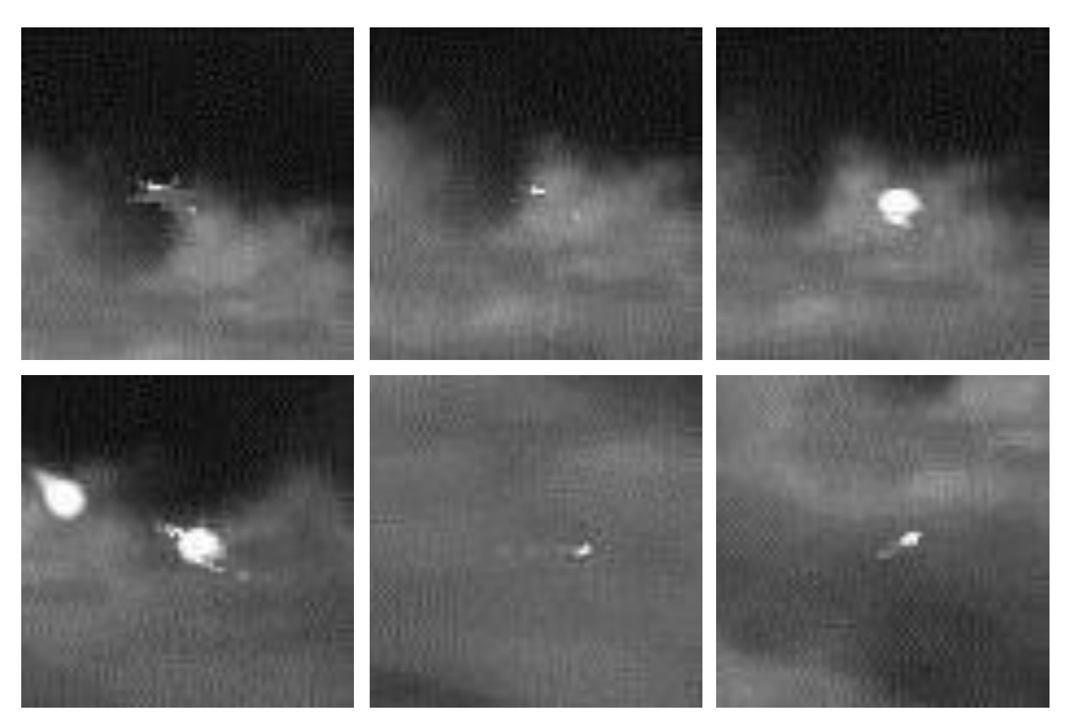
Thermal infrared technology can work under all types of weather conditions and has been widely used for rescue, surveillance, and automatic target recognition. Besides, tracking based on thermal infrared technology is not sensitive to illumination variations and can track the target in total darkness [1,2]. Airborne target tracking, which plays an important role in infrared imaging guidance, remains a challenging task [3,4]. Compared with visual tracking, the imagery generated by infrared imaging guidance has low resolution and lacks texture information [5]. Moreover, both aircraft and infrared imaging platforms are highly maneuverable, leading to strong ego-motion and severe image jittering [6]. When an aircraft passes through a cloud, the aircraft would be partly occluded by the cloud. At the same time, the infrared decoy can also lead to occlusion and radiate a stronger signal than the aircraft. The change in aircraft attitude will give rise to the difference of imaging, which is also a challenge for aircraft tracking, as seen in Figure 1.
Wang et al. [7] broke a tracker down into several parts and observed that the feature extractor plays the most important role. Thus, a robust feature representation of the aircraft is crucial to the overall performance of the tracker. Recently, trackers based on correlation filters have achieved great success [8,9,10,11], which can be effectively trained in the Fourier domain and generate dense response scores over all searching locations. With the adoption of multi-channel features [12,13] instead of single-channel gray-scale features [14], the tracking performance has been greatly improved. The progress in convolutional neural networks (CNN) inspired more research to focus on the combination of CNN features and correlation filters [15,16], which provide a further performance boost. However, the CNN features pre-trained on ImageNet are not discriminative enough for domain-specific target tracking and incur a high computational cost.
By implicitly including dense samples, the correlation filters are able to make full use of limited training data [17]. Motivated by the training mechanism of correlation filters [12,18], we explicitly construct shifted versions of the aircraft in the initial frame as the training data without requiring additional training data. To ensure a better tracking performance, we integrate handcrafted features that encode general representation into the network. The learned domain-specific features and handcrafted features can co-adapt and cooperate to achieve an objective.
The main contributions of this work are summarized as follows:
- We propose a new approach to automatically learn features online that can be adapted to the current video domain without pre-training on large datasets.
- The general feature representations and the domain-specific features learned online are integrated into a unified framework to ensure the tracking performance.
- The proposed method can be embedded in a framework based on correlation filters as a flexible module to improve the performance.
- We carry out experiments on airborne infrared imagery to demonstrate that the proposed tracking algorithm achieves competitive performance compared with benchmark trackers.
2. Related Work
Bolme et al. [14] first introduced correlation filters to visual tracking, which take single-channel gray-scale features as the input. Tracking based on the Minimum Output Sum of Squared Error (MOSSE) filters achieves competitive performance compared with the more complex trackers and runs at 669 frames per second. Henriques et al. [18] explored the circulant structure of dense samples and derived closed-form solutions with polynomial and Gaussian kernels. The introduction of the kernel trick and the exploiting of the circulant structure of the samples enable efficient training in the frequency domain, achieving orders of magnitude faster than standard methods. The Kernelized Correlation Filter (KCF) [12], which can be seen as a kernelized version of a linear correlation filter, extended the work of [18] by replacing single-channel features with Histograms of Oriented Gradients (HOGs) features [19]. The KCF [12] and the multi-channel extension of correlation filters improve the tracking performance significantly and run at hundreds of frames per second. The aforementioned trackers cannot handle scale variations well. To address the problem of scale estimation, Danelljan et al. [20] proposed to learn separate filters for scale estimation and target translation. After finding the optimal translation, scale estimation is achieved by training a classifier based on a scale pyramid. Similarly, Li et al. [13] proposed a scale adaptive scheme by defining a scaling pool. The multiple scale searching strategy and the multiple feature integration scheme work together to boost the tracking performance.
The periodic assumption of the samples implied in correlation filters enables efficient training using the Fast Fourier Transform (FFT). However, the periodic assumption also introduces undesired boundary effects, making the tracking model inaccurate. Galoogahi et al. [21] addressed the issue for single-channel discriminative correlation filters by proposing a new objective, which can reduce the samples affected by the boundary effect and can be optimized by using the Augmented Lagrangian Method (ALM). The approach limits boundary effects and preserves computational efficiency. Danelljan et al. [17] exploited a spatial regularization component to penalize correlation filter coefficients near the background to alleviate the boundary effects. The spatial regularization mitigates the attention on the background region and enhances the emphasis on the target region. The introduced component can be used for multi-dimensional features, leading to a more discriminative tracking model. Instead of learning from the circular samples, which are plagued by boundary effects, Background-Aware Correlation Filters (BACFs) [22] emphasize the learning of the tracking model from real negative samples extracted from the background. The optimization process based on the Alternating Direction Method of Multipliers (ADMM) and Sherman–Morrison lemma achieves real-time performance while maintaining competitive accuracy. Li et al. [11] incorporated temporal regularization with Spatially-Regularized Discriminative Correlation Filters (SRDCFs) [17] to handle the appearance variations of the target during the tracking process. The introduction of the temporal regularizer to SRDCF with a single sample can approximate the training of SRDCF with multiple samples, and the training can be optimized efficiently via ADMM. Dai et al. [8] proposed an adaptive spatial regularization component to obtain object-aware spatial weight. The approach can be seen as a general extension of SRDCF [17] and BACF [22]. To accelerate the tracking process, the CF model with shallow features is exploited to estimate the scale. The other correlation filters model equipped with complicated features are responsible for accurate localization.
Feature representation is a critical part of visual tracking [7,23]. Recently, convolutional neural networks have achieved great success in various vision tasks. With the adoption of CNN features, trackers based on correlation filters began to show improving performance [15,16,24]. Ma et al. [15,25] exploited the hierarchical convolutional features as target representations for visual tracking. The learned correlation filters on each layer cooperate to infer the target location in a coarse-to-fine manner. Danelljan et al. [16] extended SRDCF [17] by using CNN features and demonstrated superior performance compared to handcrafted feature representations. Further, they proposed to learn continuous convolution operators [26]. With the integration of multi-resolution feature maps in the continuous spatial domain, the tracking performance was improved. Efficient Convolution Operators (ECOs) [24] introduce a factorized convolution operator and a compact generative model of samples to the C-COT (Continuous Convolution Operators Tracking) [26] tracker, which simultaneously improves computational efficiency and tracking accuracy. He et al. [27] investigated the multi-resolution CNN features and proposed the weight sum operation of the response maps based on the ECO [24] tracker. The adoption of the first convolution layer and the final convolution layer of the VGG (Visual Geometry Group)network [28] achieves the best tracking performance. Xu et al. [29] exploited the relevance of multi-channel features and presented group feature selection in the channel and spatial dimensions. With the use of group-sparse regularization and the low-rank temporal constraint, the combination of correlation filters and CNN features provides superior tracking performance.
3. Proposed Algorithm
In this section, we first introduce feature learning via convolutional regression. Second, we detail the architecture of the network. Finally, we introduce the proposed tracking algorithm. Algorithm 1 depicts the whole process.
| Algorithm 1: Proposed tracking algorithm. |
| Input: Initial position and size of the aircraft [x0 y0 w0 h0]. Output: Estimated aircraft states [xi yi wi hi]. |
|
3.1. Learning via Convolutional Regression
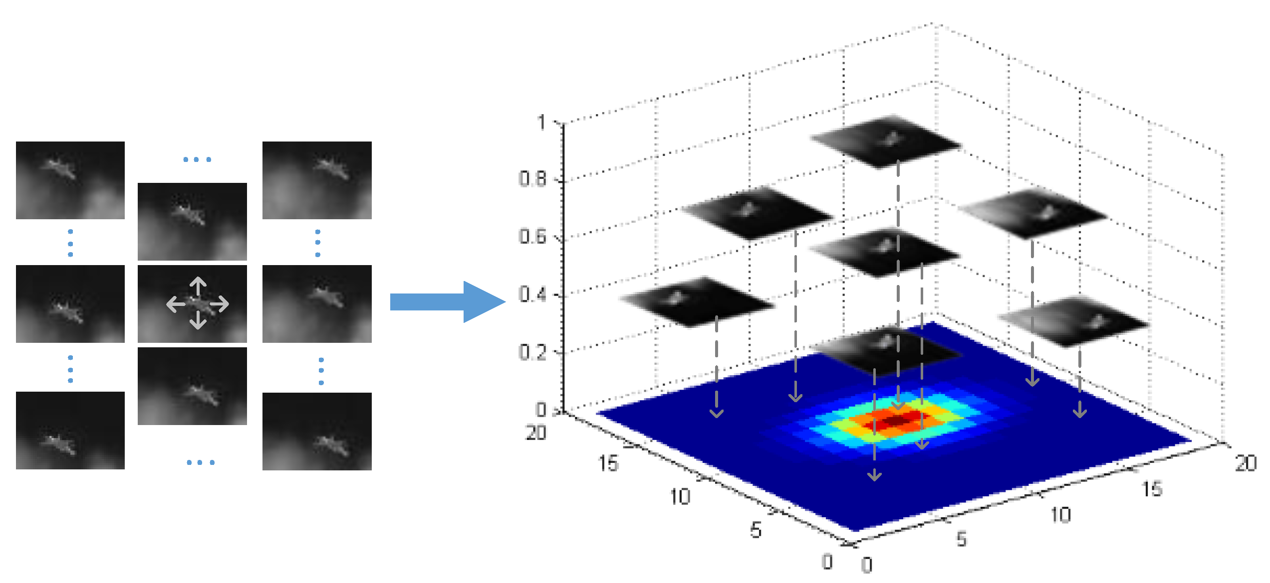
In the typical formulation of the correlation filters, the correlation filters are trained by solving a linear least-squares problem. The training samples are implicitly generated by performing a circular sliding window operation and exploiting the fast Fourier transform [12,18]. The adopted features in the correlation filters are usually handcrafted features or CNN features pre-trained on large datasets, which are not tightly bound to the current video domain. Inspired by the training mechanism of correlation filters, we explicitly construct shifted versions of the aircraft in the initial frame as the training data and try to obtain features for the current domain in a convolutional regression network. The training of the network is consistent with the training of correlation filters. Therefore, the features obtained from the network are tightly coupled with both the current video domain and the tracking frameworks based on correlation filters. Learning the weights w of the network is to minimize the following loss function,
where N is the number of shifted samples, denotes the loss of the i-th training sample , is a regularization parameter, and represents the weight decay term. The desired output for is a scalar value sampled from the Gaussian function according to its shifted position, which can be written as,
where stands for the initial position of the aircraft, represents the shifted position of the aircraft in the sample , and the variances and are proportional to the width and height of the aircraft. The correspondence between the sample and the label is shown in Figure 2.
Specifically, can be defined as the error term between the network output and the label , which is given by,
3.2. Network Architecture
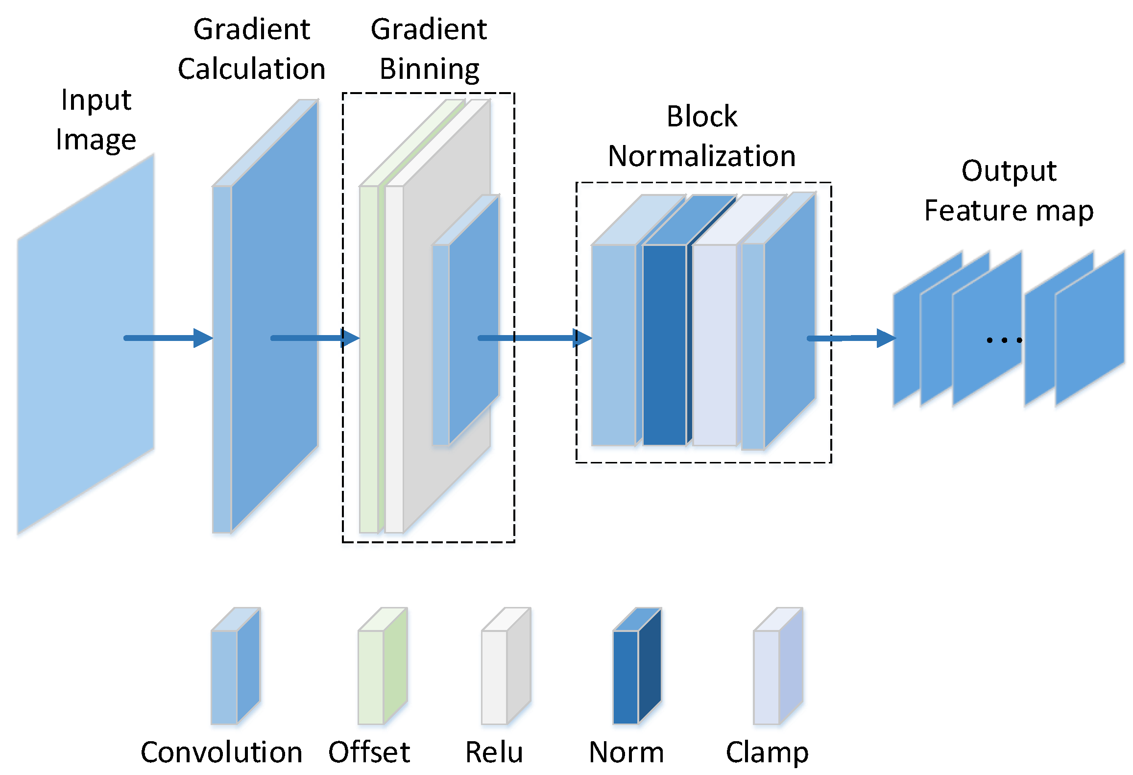
Since only a few samples extracted from the initial frame can be used as training data, to ensure better tracking performance, we incorporate general feature representations into the network. HOG features have been widely used to represent the information of the target and gain excellent performance in visual tracking [27]. To this end, we propose to combine HOG features that encode general feature representations and domain-specific features learned online into the framework. Instead of directly concatenating the HOG features and the CNN features, the way of encoding the HOG features into the network is to co-adapt and cooperate to achieve an objective. We follow the work of [31,32], which implemented the HOG features in a CNN framework. The implementation mainly includes the calculation of the gradient, the assignment of the gradient, and the normalization of the block. Firstly, the gradient along the direction is calculated using a directional filter. The k-th directional filter can be written as,
where K is the number of orientations. Then, the gradients are assigned to histogram by using an approximated bilinear binning, which is given by,
where is the projection of the gradient g along direction . The cell histogram is calculated in 8 × 8 pixels and normalized in a block composed of 2 × 2 cells. The network architecture is shown in Figure 3. The norm layer is a special case of the Local Response Normalization (LRN) layer [33], and the clamp implements the function,
where is a positive threshold. Clipping the values can avoid too much influence of very large gradients [34].
3.3. Tracking Algorithm
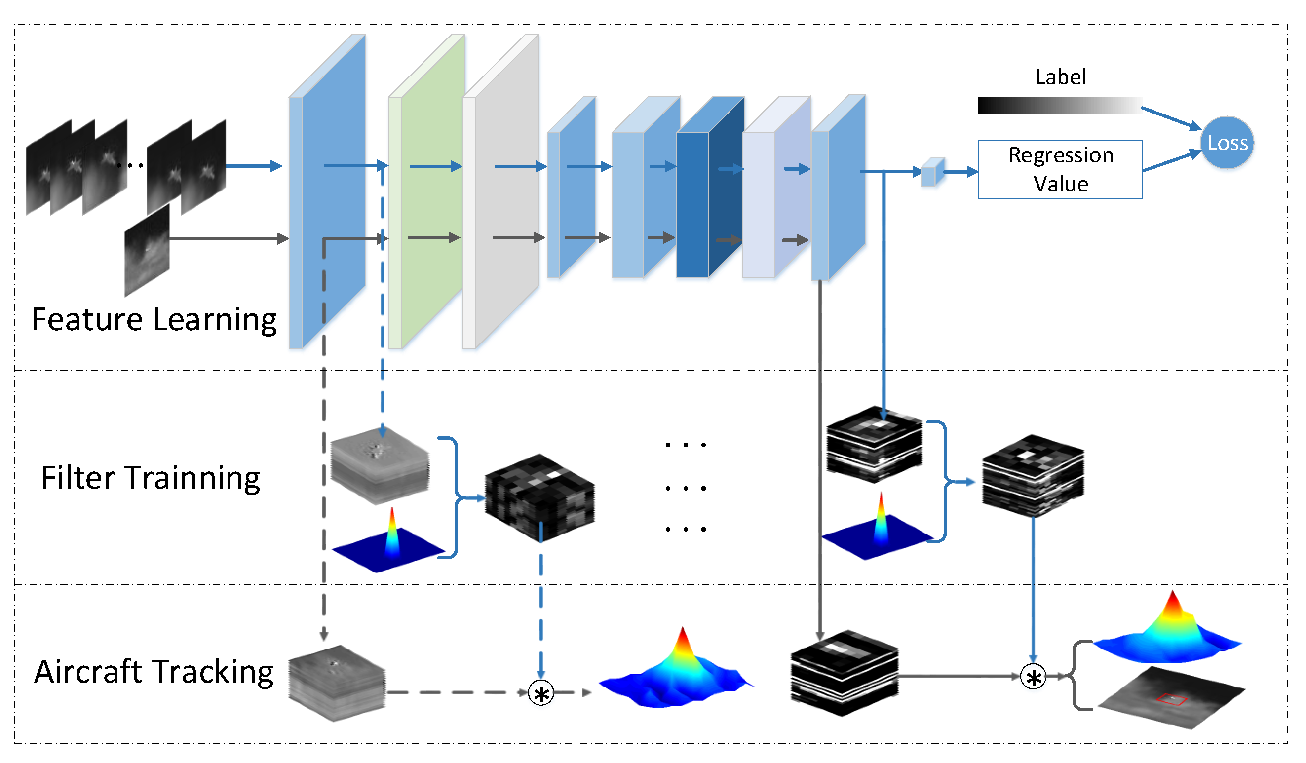
The initialization parameters of the network are obtained from the HOG features, as shown in Figure 4, and we further train the network by using Equation (1). The training process of the network is consistent with the training mechanism of correlation filters, as we mentioned in Section 3.1. After the network is trained, the feature maps from the network are integrated into the correlation filters for aircraft tracking. We denote the input image by x, and the corresponding feature is . Similarly, a correlation filter f is then learned by solving the following objective function:
where y is a Gaussian function peaked at the target center, ∗ means circular correlation, and is a regularization parameter. After, we crop a search patch and obtain the features z in the new frame. The correlation response map m can be given as,
where the hat denotes the Fourier transform, the operator denotes the inverse fast Fourier transform, ⊙ is the element-wise product, and is the complex conjugate of . Thus, the translation of the target from the previous frame can be estimated by searching for the maximum value of the correlation response map. The overall procedure of the algorithm is shown in Figure 5. We summarize the main steps of the proposed tracking algorithm in Algorithm 1.
4. Experiments
We validate the proposed method by conducting experiments on both synthetic infrared imagery and real infrared imagery. We first introduce the parameter settings of the experiments. Then, we conduct ablation studies to verify the most important part of the proposal. Finally, we compare its performance with trackers based on the tracking benchmark library.
4.1. Experimental Setup
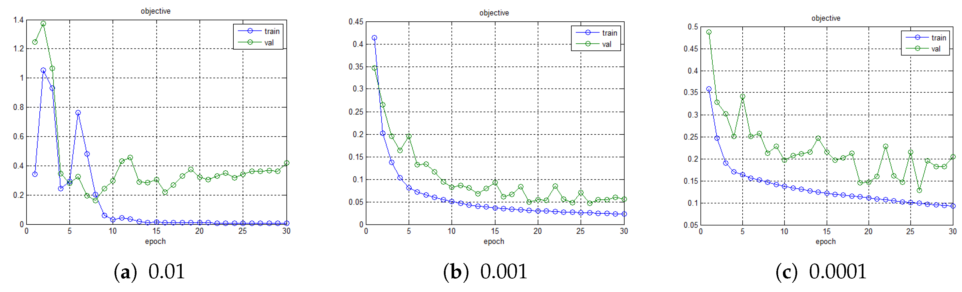
We construct shifted versions of the aircraft in the initial frame to obtain 256 training samples as the training data. The corresponding labels are assigned according to Equation (2). We follow the initial parameter settings of the network. The number of orientations is set to 18, and the threshold value in Equation (8) is 0.2. We iteratively apply the Stochastic Gradient Descent (SGD) optimizer with a batch size of 16. The setting of the learning rate is highly related to the loss curve. Therefore, we conduct learning rate experiments of different orders of magnitude and randomly select 30 percent of the samples from the training set as the validation set. The corresponding loss curves are shown in Figure 6. If the learning rate is set to 0.01, it is difficult for the loss function to converge. The loss function will converge slowly with a learning rate of 0.0001. To this end, we set the learning rate to 0.001 to make the loss function converge more smoothly and quickly. The training is stopped after 10 epochs since the loss value decreases little after that, as shown in Figure 6b. After the network is trained, the features from the network are integrated into the correlation filter tracking framework [12,24,25]. The experiments were performed on a PC with an Intel i3-4030U 1.9 GHz CPU, and 4 GB of RAM.
4.2. Ablation Studies
The features adopted in the correlation filter tracking framework play a critical role. We perform quantitative analysis to evaluate the use of features from different layers. We follow the evaluation metrics used in [35,36], which include the precision metric and the success metric, and follow the One-Pass Evaluation (OPE) protocol. The success metric is presented with plots, which show the ratios of successful frames changed with the overlap ratio between the tracked and ground-truth bounding boxes. The precision metric calculates the percentage of frames within a range of the center location error thresholds. Given tracking bounding box and ground-truth bounding box , precision P and overlap ratio R are defined as follows:
where and are the center coordinates of the tracking bounding box and ground-truth bounding box , respectively. For each frame, we can calculate the precision P and overlap ratio R. Given a precision threshold , the percentage of frames within the threshold can be computed. We change the threshold to calculate the corresponding percentage of frames. Thus, we can plot the percentage of frames varying with the threshold , which is called the precision plot. Similarly, we can plot the percentage of frames changing with the threshold to obtain the success plots. The precision score and the overlap score adopt thresholds and with 20 pixels and 0.5 to measure the percentage of the frames, which is consistent with the parameter settings in [35].
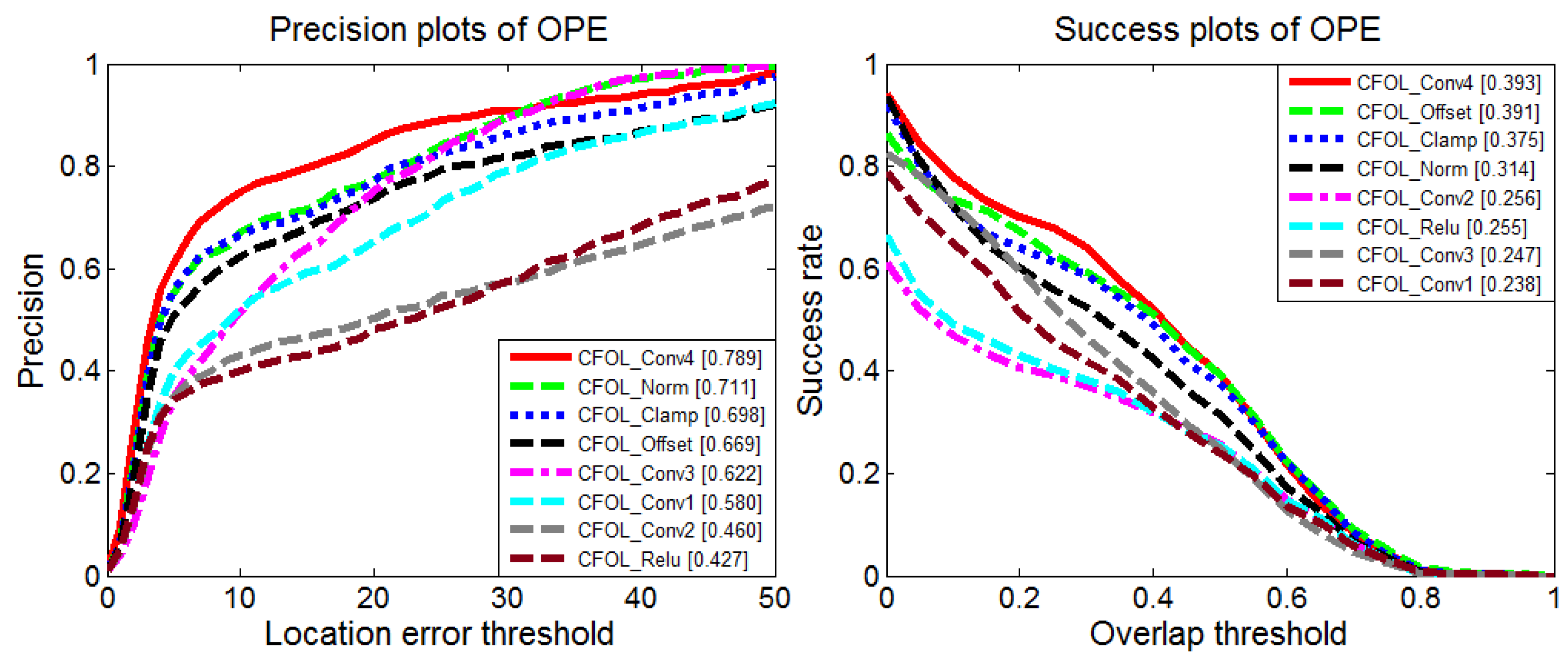
We extract features from each layer of the network to analyze the tracking performance. The experiments are performed based on the Hierarchical Convolutional Features Tracking (HCFT) framework [25]. The corresponding precision plots and success plots are shown in Figure 7. The results are obtained based on synthetic infrared imagery, composing of simulated aircraft and a real cloud background. The dataset is collected by the Institute of Flight Control and Simulation Technology. The features from the latter layers achieve better performance. Therefore, the features of the last layer are adopted in our subsequent experiments.
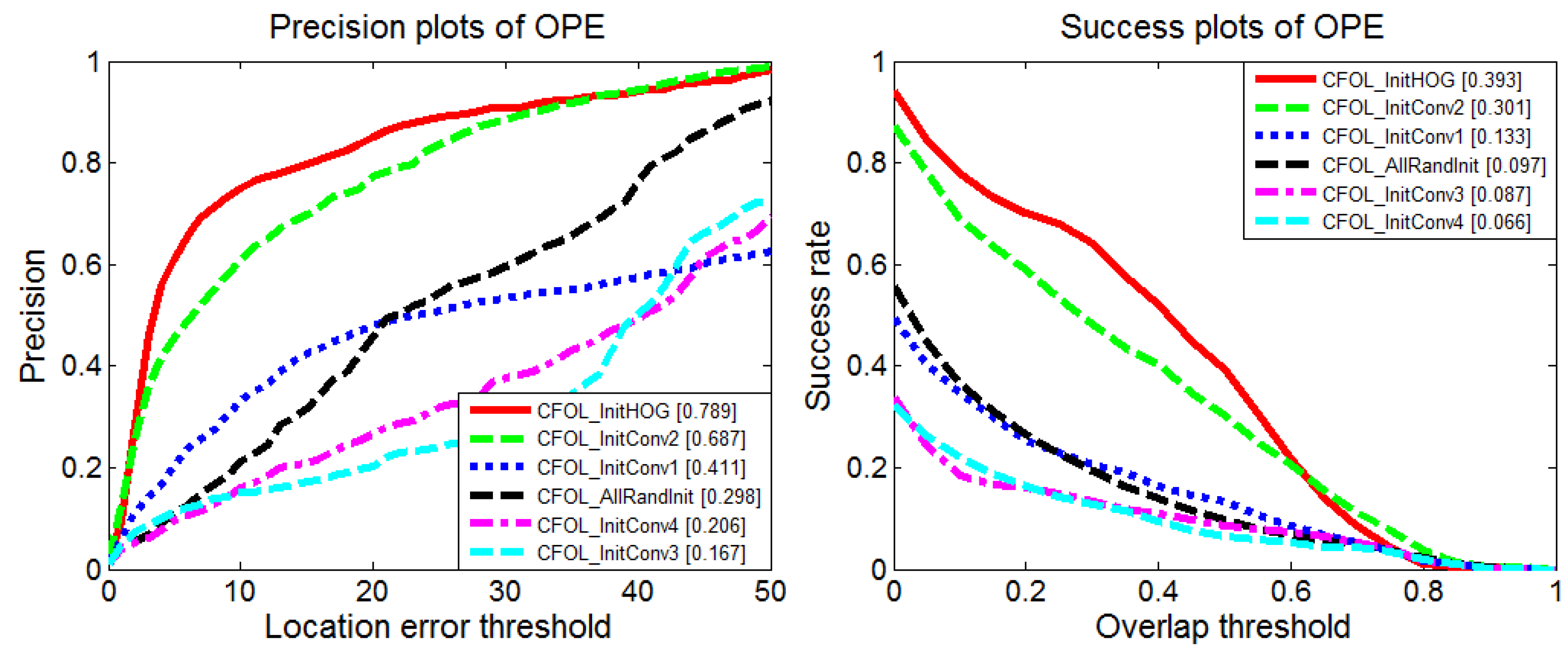
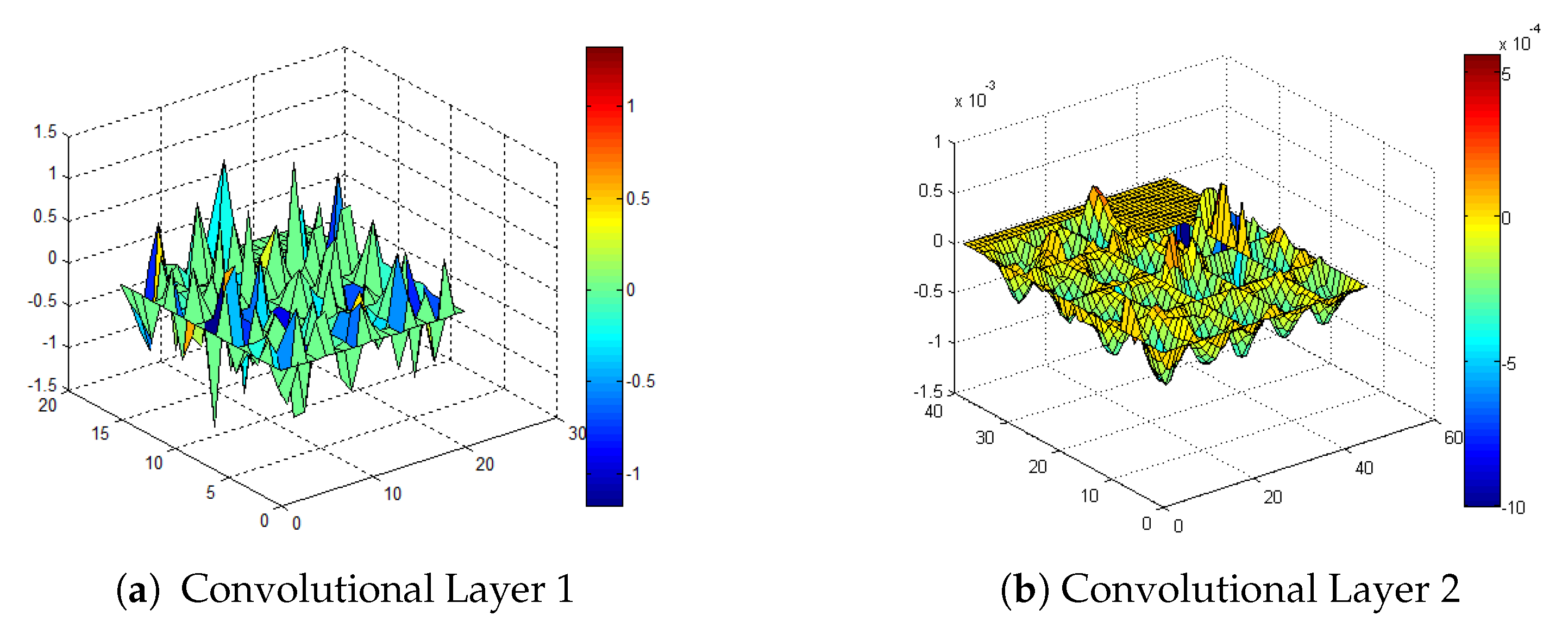
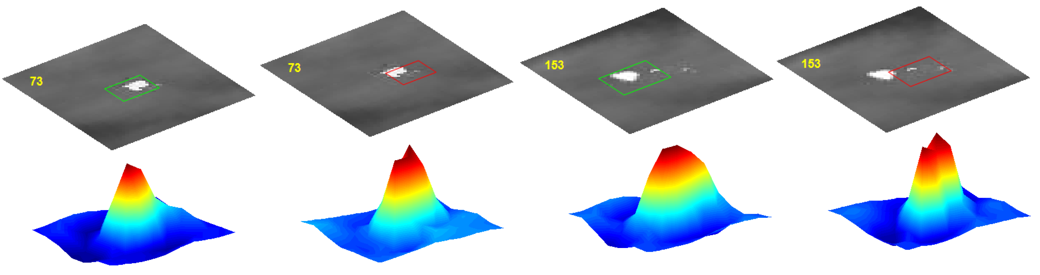
To evaluate the effect of the initialization of the weights with the computation of the HOG features, we perform experiments including random initialization of all the convolutional layers and initialize the weights of the first to fourth convolutional layer with the HOG features in turn. The performance comparisons with different initialization parameters are shown in Figure 8. As we can see, the initialization of the second convolutional layer with the HOG features improves the performance greatly. For better analysis of the weights after training, we visualize the changes of the first and second convolutional layer after training with initialization parameters obtained from the HOG features. As shown in Figure 9, the second convolutional layer shows slight changes, which also proves the importance of its initialization. Its main distribution is kept after training. The training process with parameters from the HOG features acts like the fine-tuning parameters for the current video domain. The best results are achieved by initializing all layers with the HOG features. The tracking results using the HOG features (tracking boxes with green borders) and the features after training (tracking boxes with red borders) are shown in Figure 10. If we adopt the HOG features alone, the tracker begins to drift to the suspected region, caused by decoy interference. After training the network for the current video domain with the initialization parameters of the HOG features, the tracker learns more discriminative features. As shown in Figure 10, the maximum value of the response maps points to the target region. Thus, the combination of the training with the parameters of the HOG features achieves better performance.
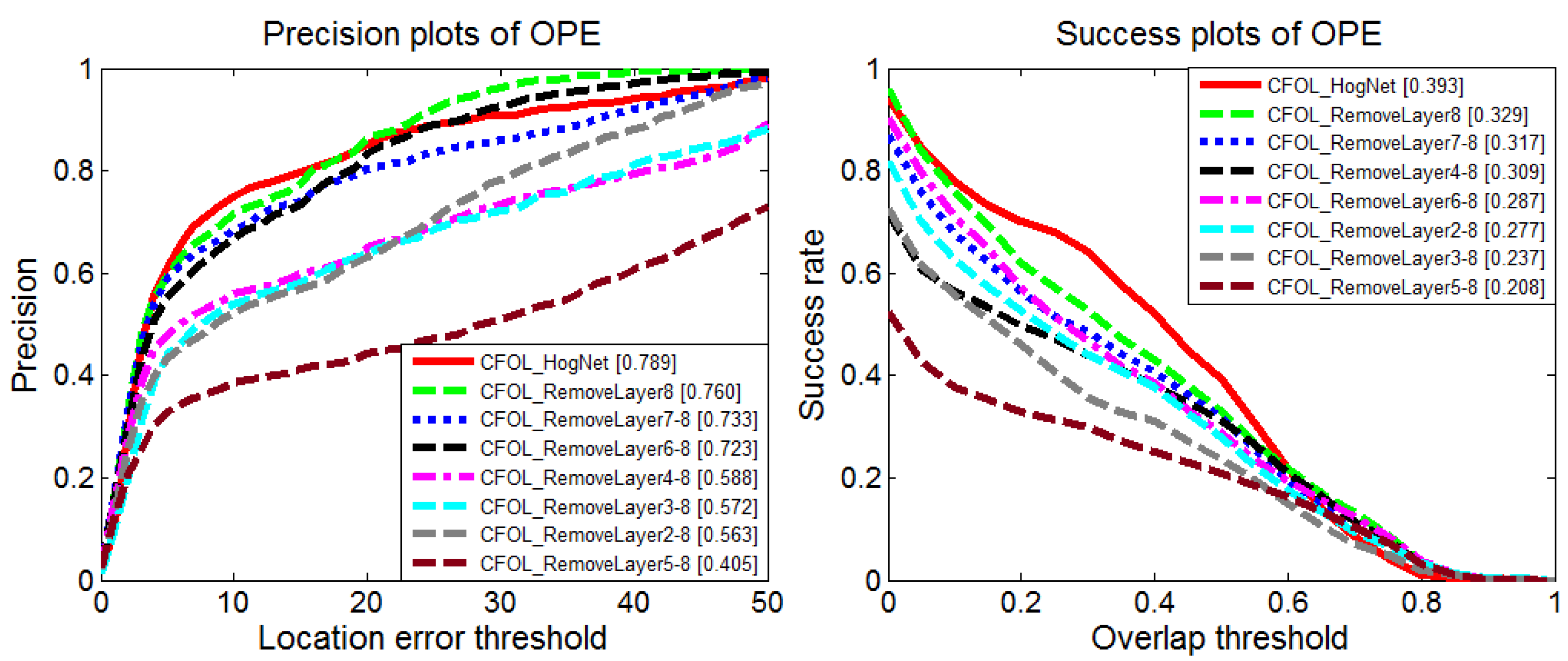
Furthermore, we conduct experiments with different networks to verify the effect of the architecture. We manually remove different layers from the original network and adopt the features of the last layer for comparison. The performance degrades after removing layers, as shown in Figure 11. The performance boost benefits from the combination of the network architecture and the initialization parameters obtained from the HOG features.
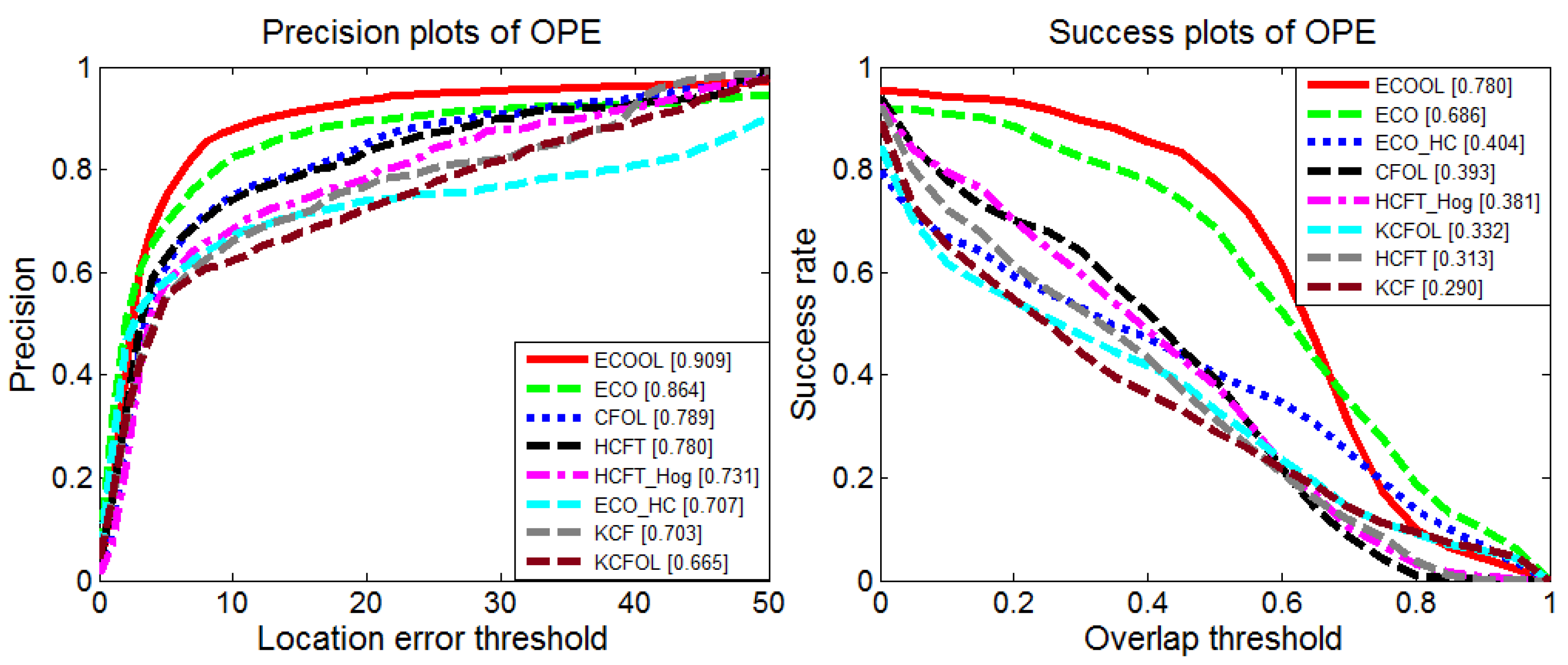
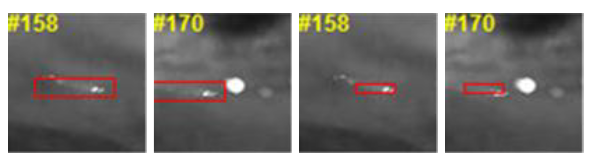
To further analyze the effectiveness of the feature learning module, we integrate the module into different frameworks based on the correlation filters and compare the tracking performance with different baselines. The experiments are conducted based on the KCF framework [12], HCFT framework [25], and ECO framework [24]. Then, these trackers with the online learning modules are named KCFOL (Kernelized Correlation Filter with Online Learning), CFOL (Convolutional Features with Online Learning), and ECOOL (Efficient Convolution Operator with Online Learning), respectively. On the basis of the experimental results stated above, KCFOL, CFOL, and ECOOL are equipped with features of the fourth convolutional layer. The evaluation includes the features learned online (ECOOL, CFOL, KCFOL), the features extracted from VGG-Net [28] (HCFT, ECO), and the HOG features (ECO-HC KCF, HCFT-HOG). As seen from Figure 12, the ECO tracker benefits greatly from the integration of the online learning module (ECOOL), while the KCF tracker does not gain many benefits from the embedding module. We visualize the tracking result of the ECOOL tracker and KCFOL tracker. As the target approaches, there exist changes in the scale of the target. Since the KCF tracker has no scale estimation module, the tracking results focus on the local region of the target and cannot achieve a good feature representation of the target model. The tracking bounding box easily drifts to the suspected area. The scale estimation method adopted in the ECO tracker can handle the challenge of scale change, leading to a better feature representation of the target model and superior tracking performance, as seen from Figure 13.
4.3. Evaluating the Tracking Benchmark
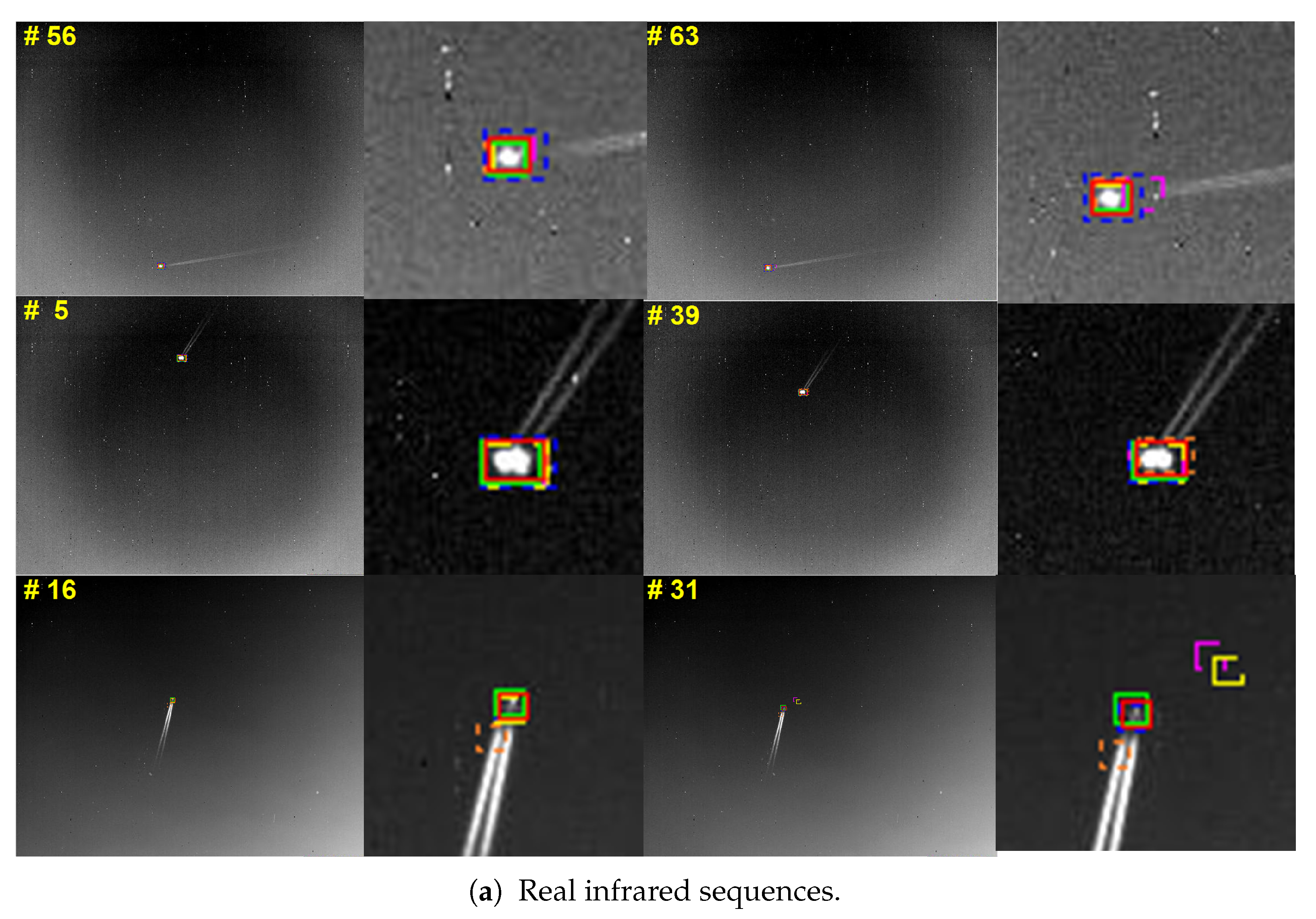
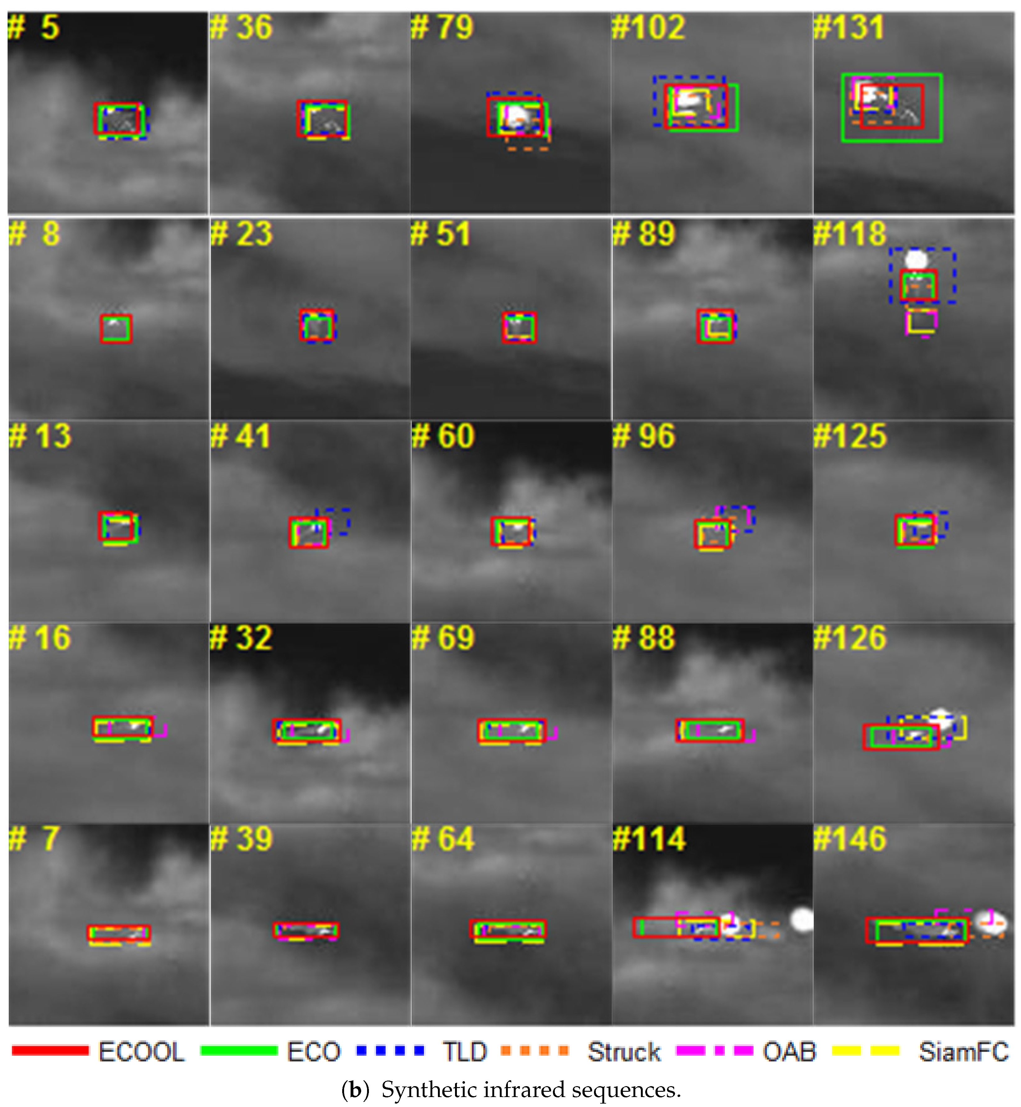
The former experiments were conducted on synthetic infrared imagery, composed of simulated aircraft and a real cloud background. The aircraft was simulated based on the OpenScene-Graph (OSG) toolkit and was rendered according to its infrared signatures [37,38,39,40]. The generation of the simulated image was integrated with the navigation and guidance processes of the missile. The image of the real cloud was captured by an IRCAM Equus 327 KM. The infrared camera worked in the band of 3–5 μm, with a resolution of 640 × 512 pixels. To demonstrate the effectiveness of our aircraft-tracking algorithm, we conducted the following experiments on both synthetic infrared imagery and real infrared imagery based on the tracking benchmark library [35]. The comparison includes ECO [24], HCFT [15], SiamRPN (Siamese Region Proposal Network) [41], SiamFC (Fully-Convolutional Siamese Networks) [42], and the trackers in the tracking benchmark library [35]. The relevant methods for comparison are summarized as follows.
CF based trackers are trained by solving a linear least-squares problem. The periodic assumption of the samples implied by correlation filters enables efficient training using the fast Fourier transform and can generate a dense response. In the process of implementation, KCF [12] adopts HOG features, while HCFT [15] and ECO [24] adopt CNN features pre-trained from VGG-Net [28]. KCF, HCFT, and ECO are implemented using MATLAB.
Boosting based trackers consider tracking as a binary classification problem and combine weak classifiers into a strong classifier. OAB (Online Adaptive Boosting) [43] adopts Haar features, orientation histograms, and local binary patterns to generate weak classifiers. To alleviate the drift problem introduced by the online update of the ensemble of classifiers, SemiT (Semi-supervised Tracking) [44] formulates the update process in a semi-supervised fashion, which utilizes both label data and unlabeled samples collected during tracking. The implementations of OAB and SemiT are achieved by using the C language.
TLD (Tracking-Learning-Detection) [45] uses positive and negative constraints to restrict the labeling of the unlabeled samples, which in turn guides the training of the binary classifier. The constraints are implemented via Lucas–Kanade and the Normalized Cross-Correlation (NCC). To reduce the dependence on generating training samples from unlabeled data, Struck [46] uses a kernelized structured output support vector machine to directly predict the change in object location. The features adopted in TLD and Struck are binary patterns and Haar features, respectively. Besides, TLD is implemented using MATLAB and the C language, while Struck is carried out using the C language.
The trackers adopt features with sparse representation expressing a target by a sparse linear combination of a few trivial templates. In this category, the L1APG (L1 Accelerated Proximal Gradient) [47] tracker adopts the holistic representation and tracks the object by solving the L1 minimization problem. ASLA (Adaptive Structural Local Appearance) [48] utilizes a structural local sparse model and alignment-pooling method across the local patches to measure the similarity between the candidate regions and the target model. They are implemented within the particle filter framework, and the optimal state can be computed by the maximum a posteriori estimation. In the implementation, L1APG and ASLA are conducted via the MATLAB platform.
The Siamese network consists of two branches, and the parameters between the two branches are tied to apply an identical transformation to the exemplar image and the candidate image. SiamFC [42] formulates tracking as learning similarity functions. In a more specific implementation, the similarity functions are trained from ImageNet Video with the convolutional features of AlexNet [33]. SiamRPN [41] adopts the region proposal network instead of the multi-scale test adopted in SiamFC to obtain a better estimation of the scale. The training set of SiamRPN includes ImageNet Video and YouTube-BB (Youtube Bounding Boxes)[49]. The implementations of SiamFC and SiamRPN are performed through MatConvNet (MATLAB toolbox implementing Convolutional Networks)and Pytorch, respectively. The codes of KCF, OAB, SemiT, TLD, Struck, L1APG, and ASLA are provided in the tracking benchmark library [35], and the codes of HCFT, ECO, SiamFC, and SiamRPN are provided by the authors.
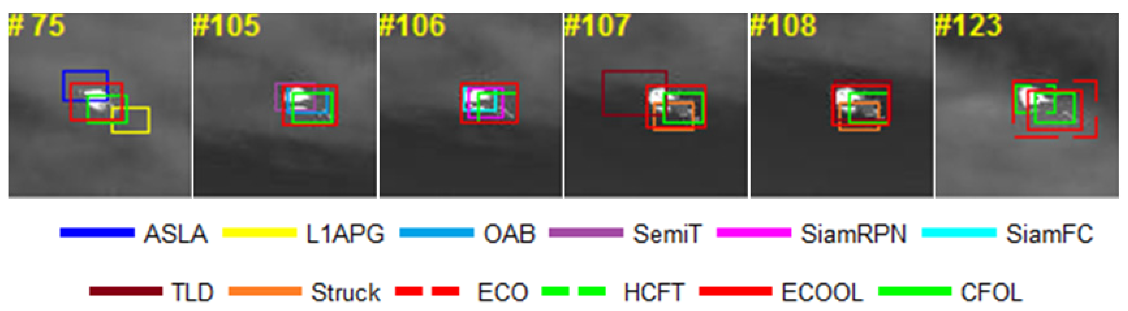
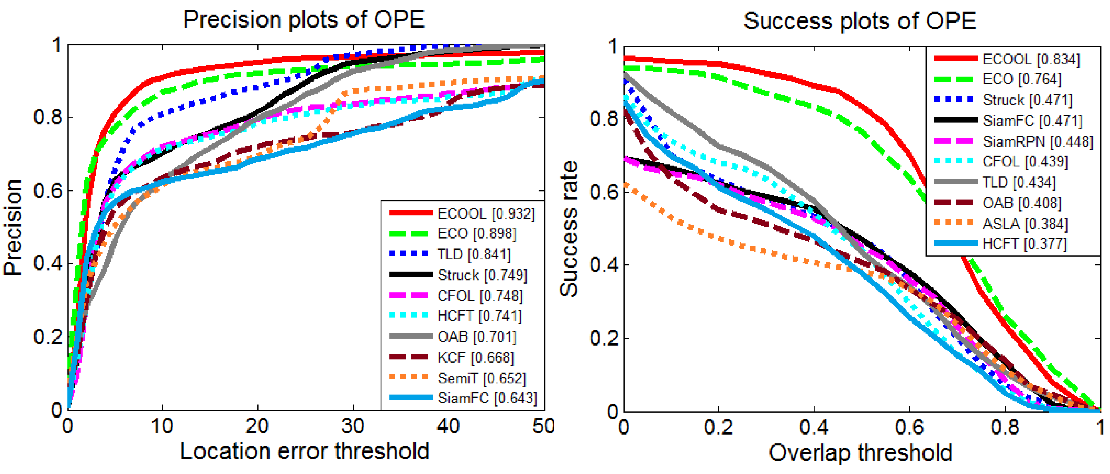
The evaluation follows the OPE protocol used in [35], and the details of the dataset used in the experiments are listed in Table 2. The evaluated tracking algorithms are summarized in Table 3. Trackers with dense sampling (TLD, Struck) provide a large search range and achieve better performance. Among the evaluation results, discriminative trackers (ECO [24], TLD [45], Struck [46]) perform better than trackers based on generative models (L1APG [47], ASLA [48]). Discriminative trackers employ the information from both the target and background and train a classifier to distinguish the target from the background [7]. For generative model based trackers, it is difficult to learn the generative appearance model of the target in the complex background. For aircraft tracking in infrared imagery, the aircraft may be frequently occluded by a cloud or an infrared decoy, resulting in inaccurate target models. As seen from Figure 14, ASLA and L1APG drift to the decoy and the cloud in Frame 75. The online update of the ensemble of weak classifiers helps distinguish the target from the background, but it also introduces errors due to frequent updates. SiamRPN and SiamFC benefit from the large training dataset to learn similarity functions. However, they lack an efficient model update mechanism to handle the appearance change, leading to model drift problems. Notice that in Frame 107, TLD lost the target. However, in Frame 108, TLD is re-initialized by its detector and successfully locks onto the target again. Both HCFT and ECO adopt CNN features to improve the performance. Instead of simply resampling all feature channels at the same resolution, ECO adopts continuous convolution operators to integrate feature channels, which enables more accurate localization. After replacing the pre-trained CNN feature with online learning features (CFOL, ECOOL), the performance of the baseline methods are improved. The overall performance is summarized by precision plots and success plots. For clarity, only the top 10 trackers are presented, as shown in Figure 15. Qualitative comparisons with the top-performing trackers are shown in Figure 16.
5. Conclusions
In this paper, we propose an effective algorithm for aircraft tracking in infrared imagery. We integrate domain-specific features learned online and general feature representations in a unified convolutional network. The training of the network is consistent with the training mechanism of the correlation filters. Therefore, the features learned are closely related to both the current video domain and the trackers based on correlation filters. The introduced feature learning method can be integrated into the tracking framework as a flexible module to improve the baseline method. Experimental results show that the proposed algorithm achieves competitive performance in terms of accuracy and robustness.
Author Contributions
S.W. designed the algorithm, conducted the experiments, and wrote the paper. S.L. analyzed the data and assisted in writing the manuscript. K.Z. and J.Y. supervised the study and reviewed this paper. All authors read and agreed to the published version of the manuscript.
Funding
This research was funded by the National Natural Science Foundation of China under Grant Number 61703337 and the Aerospace Science and Technology Innovation Fund of China under Grant Number SAST2017-082.
Acknowledgments
The authors would like to thank the provision of the infrared image sequences simulated by the Institute of Flight Control and Simulation Technology.
Conflicts of Interest
The authors declare no conflict of interest.
References
- Li, X.; Liu, Q.; Fan, N.; He, Z.; Wang, H. Hierarchical spatial-aware Siamese network for thermal infrared object tracking. Knowl.-Based Syst. 2019, 166, 71–81. [Google Scholar] [CrossRef] [Green Version]
- Liu, Q.; Lu, X.; He, Z.; Zhang, C.; Chen, W.S. Deep convolutional neural networks for thermal infrared object tracking. Knowl.-Based Syst. 2017, 134, 189–198. [Google Scholar] [CrossRef]
- Zaveri, M.A.; Merchant, S.N.; Desai, U.B. Air-borne approaching target detection and tracking in infrared image sequence. In Proceedings of the 2004 International Conference on Image Processing (ICIP’04), Singapore, 24–27 October 2004; Volume 2, pp. 1025–1028. [Google Scholar] [CrossRef]
- Wan, M.; Gu, G.; Qian, W.; Ren, K.; Chen, Q.; Zhang, H.; Maldague, X. Total Variation Regularization Term-Based Low-Rank and Sparse Matrix Representation Model for Infrared Moving Target Tracking. Remote Sens. 2018, 10, 510. [Google Scholar] [CrossRef] [Green Version]
- Wan, M.; Gu, G.; Qian, W.; Ren, K.; Chen, Q.; Maldague, X. Infrared Image Enhancement Using Adaptive Histogram Partition and Brightness Correction. Remote Sens. 2018, 10, 682. [Google Scholar] [CrossRef] [Green Version]
- del Blanco, C.R.; Jaureguizar, F.; García, N.; Salgado, L. Robust automatic target tracking based on a Bayesian ego-motion compensation framework for airborne FLIR imagery. In Proceedings of the Automatic Target Recognition XIX, International Society for Optics and Photonics, Orlando, FL, USA, 13–14 April 2009; Volume 7335, p. 733514. [Google Scholar] [CrossRef] [Green Version]
- Wang, N.; Shi, J.; Yeung, D.Y.; Jia, J. Understanding and diagnosing visual tracking systems. In Proceedings of the IEEE International Conference on Computer Vision, Santiago, Chile, 7–13 December 2015; pp. 3101–3109. [Google Scholar]
- Dai, K.; Wang, D.; Lu, H.; Sun, C.; Li, J. Visual Tracking via Adaptive Spatially-Regularized Correlation Filters. In Proceedings of the IEEE Conference on Computer Vision and Pattern Recognition, Long Beach, CA, USA, 15–20 June 2019; pp. 4670–4679. [Google Scholar]
- Sun, Y.; Sun, C.; Wang, D.; He, Y.; Lu, H. ROI Pooled Correlation Filters for Visual Tracking. In Proceedings of the IEEE Conference on Computer Vision and Pattern Recognition, Long Beach, CA, USA, 15–20 June 2019; pp. 5783–5791. [Google Scholar]
- Zhang, M.; Wang, Q.; Xing, J.; Gao, J.; Peng, P.; Hu, W.; Maybank, S. Visual tracking via spatially aligned correlation filters network. In Proceedings of the European Conference on Computer Vision (ECCV), Munich, Germany, 8–14 September 2018; pp. 469–485. [Google Scholar]
- Li, F.; Tian, C.; Zuo, W.; Zhang, L.; Yang, M.H. Learning spatial-temporal regularized correlation filters for visual tracking. In Proceedings of the IEEE Conference on Computer Vision and Pattern Recognition, Salt Lake City, UT, USA, 18–22 June 2018; pp. 4904–4913. [Google Scholar]
- Henriques, J.F.; Caseiro, R.; Martins, P.; Batista, J. High-speed tracking with kernelized correlation filters. IEEE Trans. Pattern Anal. Mach. Intell. 2015, 37, 583–596. [Google Scholar] [CrossRef] [PubMed] [Green Version]
- Li, Y.; Zhu, J. A scale adaptive kernel correlation filter tracker with feature integration. In Proceedings of the European Conference on Computer Vision, Zurich, Switzerland, 6–12 September 2014; pp. 254–265. [Google Scholar]
- Bolme, D.S.; Beveridge, J.R.; Draper, B.A.; Lui, Y.M. Visual object tracking using adaptive correlation filters. In Proceedings of the 2010 IEEE Computer Society Conference on Computer Vision and Pattern Recognition, San Francisco, CA, USA, 13–18 June 2010; pp. 2544–2550. [Google Scholar]
- Ma, C.; Huang, J.B.; Yang, X.; Yang, M.H. Robust visual tracking via hierarchical convolutional features. IEEE Trans. Pattern Anal. Mach. Intell. 2018, 41, 2709–2723. [Google Scholar] [CrossRef] [PubMed] [Green Version]
- Danelljan, M.; Hager, G.; Shahbaz Khan, F.; Felsberg, M. Convolutional features for correlation filter based visual tracking. In Proceedings of the IEEE International Conference on Computer Vision Workshops, Santiago, Chile, 7–13 December 2015; pp. 58–66. [Google Scholar]
- Danelljan, M.; Hager, G.; Shahbaz Khan, F.; Felsberg, M. Learning spatially regularized correlation filters for visual tracking. In Proceedings of the IEEE International Conference on Computer Vision, Santiago, Chile, 7–13 December 2015; pp. 4310–4318. [Google Scholar]
- Henriques, J.F.; Caseiro, R.; Martins, P.; Batista, J. Exploiting the circulant structure of tracking-by-detection with kernels. In Proceedings of the European Conference on Computer Vision, Florence, Italy, 7–13 October 2012; pp. 702–715. [Google Scholar]
- Dalal, N.; Triggs, B. Histograms of oriented gradients for human detection. In Proceedings of the 2005 IEEE computer society conference on computer vision and pattern recognition (CVPR’05), San Diego, CA, USA, 20–26 June 2005; Volume 1, pp. 886–893. [Google Scholar]
- Danelljan, M.; Häger, G.; Khan, F.; Felsberg, M. Accurate scale estimation for robust visual tracking. In Proceedings of the British Machine Vision Conference, Nottingham, UK, 1–5 September 2014. [Google Scholar]
- Kiani Galoogahi, H.; Sim, T.; Lucey, S. Correlation filters with limited boundaries. In Proceedings of the IEEE Conference on Computer Vision and Pattern Recognition, Boston, MA, USA, 7–12 June 2015; pp. 4630–4638. [Google Scholar]
- Kiani Galoogahi, H.; Fagg, A.; Lucey, S. Learning background-aware correlation filters for visual tracking. In Proceedings of the IEEE International Conference on Computer Vision, Venice, Italy, 22–29 October 2017; pp. 1135–1143. [Google Scholar]
- Song, Y.; Ma, C.; Gong, L.; Zhang, J.; Lau, R.W.; Yang, M.H. Crest: Convolutional residual learning for visual tracking. In Proceedings of the IEEE International Conference on Computer Vision, Venice, Italy, 22–29 October 2017; pp. 2555–2564. [Google Scholar]
- Danelljan, M.; Bhat, G.; Khan, F.S.; Felsberg, M. ECO: Efficient Convolution Operators for Tracking. In Proceedings of the CVPR, Honolulu, HI, USA, 21–26 July 2017; Volume 1, p. 3. [Google Scholar]
- Ma, C.; Huang, J.B.; Yang, X.; Yang, M.H. Hierarchical convolutional features for visual tracking. In Proceedings of the IEEE International Conference on Computer Vision, Santiago, Chile, 7–13 December 2015; pp. 3074–3082. [Google Scholar]
- Danelljan, M.; Robinson, A.; Khan, F.S.; Felsberg, M. Beyond correlation filters: Learning continuous convolution operators for visual tracking. In Proceedings of the European Conference on Computer Vision, Amsterdam, The Netherlands, 8–16 October 2016; pp. 472–488. [Google Scholar]
- He, Z.; Fan, Y.; Zhuang, J.; Dong, Y.; Bai, H. Correlation filters with weighted convolution responses. In Proceedings of the IEEE International Conference on Computer Vision Workshops, Venice, Italy, 22–29 October 2017; pp. 1992–2000. [Google Scholar]
- Simonyan, K.; Zisserman, A. Very deep convolutional networks for large-scale image recognition. arXiv 2014, arXiv:1409.1556. [Google Scholar]
- Xu, T.; Feng, Z.H.; Wu, X.J.; Kittler, J. Joint group feature selection and discriminative filter learning for robust visual object tracking. In Proceedings of the IEEE International Conference on Computer Vision, Seoul, Korea, 27 October 27–2 November 2019; pp. 7950–7960. [Google Scholar]
- Chen, K.; Tao, W. Convolutional regression for visual tracking. IEEE Trans. Image Process. 2018, 27, 3611–3620. [Google Scholar] [CrossRef] [PubMed] [Green Version]
- Mahendran, A.; Vedaldi, A. Understanding deep image representations by inverting them. In Proceedings of the IEEE Conference on Computer Vision and Pattern Recognition, Boston, MA, USA, 7–12 June 2015; pp. 5188–5196. [Google Scholar]
- Mahendran, A.; Vedaldi, A. Visualizing deep convolutional neural networks using natural pre-images. Int. J. Comput. Vis. 2016, 120, 233–255. [Google Scholar] [CrossRef] [Green Version]
- Krizhevsky, A.; Sutskever, I.; Hinton, G.E. Imagenet classification with deep convolutional neural networks. Commun. ACM 2017, 60, 84–90. [Google Scholar] [CrossRef]
- Tomasi, C. Histograms of oriented gradients. Comput. Vis. Sampl. 2012, 1, 1–6. [Google Scholar]
- Wu, Y.; Lim, J.; Yang, M.H. Object tracking benchmark. IEEE Trans. Pattern Anal. Mach. Intell. 2015, 37, 1834–1848. [Google Scholar] [CrossRef] [PubMed] [Green Version]
- Liu, S.; Liu, D.; Srivastava, G.; Połap, D.; Woźniak, M. Overview of correlation filter based algorithms in object tracking. Complex Intell. Syst. 2020, 1, 1–23. [Google Scholar]
- Wu, S.; Zhang, K.; Niu, S.; Yan, J. Anti-Interference Aircraft-Tracking Method in Infrared Imagery. Sensors 2019, 19, 1289. [Google Scholar] [CrossRef] [PubMed] [Green Version]
- Lepage, J.F.; Labrie, M.A.; Rouleau, E.; Richard, J.; Ross, V.; Dion, D.; Haarison, N. DRDC’s approach to IR scene generation for IRCM simulation. In Proceedings of the Technologies for Synthetic Environments: Hardware-in-the-Loop XVI, International Society for Optics and Photonics, Orlando, FL, USA, 27–28 April 2011; Volume 8015, p. 80150F. [Google Scholar] [CrossRef]
- Le Goff, A.; Cathala, T.; Latger, J. New impressive capabilities of SE-workbench for EO/IR real-time rendering of animated scenarios including flares. In Proceedings of the Target and Background Signatures. International Society for Optics and Photonics, Toulouse, France, 23–24 September 2015; Volume 9653, p. 965307. [Google Scholar] [CrossRef]
- Willers, C.J.; Willers, M.S.; Lapierre, F. Signature modelling and radiometric rendering equations in infrared scene simulation systems. In Proceedings of the Technologies for Optical Countermeasures VIII. International Society for Optics and Photonics, Prague, Czech Republic, 21–22 September 2011; Volume 8187, p. 81870R. [Google Scholar] [CrossRef]
- Li, B.; Yan, J.; Wu, W.; Zhu, Z.; Hu, X. High performance visual tracking with siamese region proposal network. In Proceedings of the IEEE Conference on Computer Vision and Pattern Recognition, Salt Lake City, UT, USA, 18–23 June 2018; pp. 8971–8980. [Google Scholar]
- Bertinetto, L.; Valmadre, J.; Henriques, J.F.; Vedaldi, A.; Torr, P.H. Fully-convolutional siamese networks for object tracking. In Proceedings of the European Conference on Computer Vision, Amsterdam, The Netherlands, 8–16 October 2016; pp. 850–865. [Google Scholar]
- Grabner, H.; Grabner, M.; Bischof, H. Real-time tracking via on-line boosting. Bmvc 2006, 1, 6. [Google Scholar]
- Grabner, H.; Leistner, C.; Bischof, H. Semi-supervised on-line boosting for robust tracking. In Proceedings of the European Conference on Computer Vision, Marseille, France, 12–18 October 2008; pp. 234–247. [Google Scholar]
- Kalal, Z.; Matas, J.; Mikolajczyk, K. Pn learning: Bootstrapping binary classifiers by structural constraints. In Proceedings of the 2010 IEEE Computer Society Conference on Computer Vision and Pattern Recognition, San Francisco, CA, USA, 13–18 June 2010; pp. 49–56. [Google Scholar]
- Hare, S.; Golodetz, S.; Saffari, A.; Vineet, V.; Cheng, M.M.; Hicks, S.L.; Torr, P.H. Struck: Structured output tracking with kernels. IEEE Trans. Pattern Anal. Mach. Intell. 2015, 38, 2096–2109. [Google Scholar] [CrossRef] [PubMed] [Green Version]
- Bao, C.; Wu, Y.; Ling, H.; Ji, H. Real time robust l1 tracker using accelerated proximal gradient approach. In Proceedings of the 2012 IEEE Conference on Computer Vision and Pattern Recognition, Providence, RI, USA, 16–21 June 2012; pp. 1830–1837. [Google Scholar]
- Jia, X.; Lu, H.; Yang, M.H. Visual tracking via adaptive structural local sparse appearance model. In Proceedings of the 2012 IEEE Conference on Computer Vision and Pattern Recognition, Providence, RI, USA, 16–21 June 2012; pp. 1822–1829. [Google Scholar]
- Real, E.; Shlens, J.; Mazzocchi, S.; Pan, X.; Vanhoucke, V. Youtube-boundingboxes: A large high-precision human-annotated data set for object detection in video. In Proceedings of the IEEE Conference on Computer Vision and Pattern Recognition, Honolulu, HI, USA, 22 October 2017; pp. 5296–5305. [Google Scholar]
Figure 1.
The challenge of airborne infrared target tracking. The aircraft is partly occluded by the cloud and the infrared decoy. Meanwhile, the appearance of the aircraft will frequently change due to pose variation.
Figure 1.
The challenge of airborne infrared target tracking. The aircraft is partly occluded by the cloud and the infrared decoy. Meanwhile, the appearance of the aircraft will frequently change due to pose variation.

Figure 2.
The correspondence between samples and labels. The labels are sampled from the Gaussian function.
Figure 2.
The correspondence between samples and labels. The labels are sampled from the Gaussian function.

Figure 3.
The architecture of the network. The parameter settings of the convolutional layers are shown in Table 1. The offset layer and the Rectified Linear Unit (ReLU) layer are implemented according to Equation (7). The norm layer normalizes the values to reduce the effect of changes in contrast. The layer of the clamp limits the maximum values to .

Figure 4.
Visualization of the initial parameters of the convolutional layers.

Figure 5.
The procedure of the proposed tracker. The process of feature learning is achieved by training the network based on Equation (1). The learned features are integrated into the correlation filter tracking framework.
Figure 5.
The procedure of the proposed tracker. The process of feature learning is achieved by training the network based on Equation (1). The learned features are integrated into the correlation filter tracking framework.

Figure 6.
The loss curves with different learning rates.

Figure 7.
Performance comparison using features from different layers. OPE, One-Pass Evaluation. CFOL: Convolutional Features with Online Learning.
Figure 7.
Performance comparison using features from different layers. OPE, One-Pass Evaluation. CFOL: Convolutional Features with Online Learning.

Figure 8.
Performance comparison with different initialization parameters.

Figure 9.
The changes of the first and second convolutional layers.

Figure 10.
Visualization of the tracking results.

Figure 11.
Performance comparison with different network architectures.

Figure 12.
Baseline comparison using different features. ECO, Efficient Convolution Operator; HCFT, Hierarchical Convolutional Features Tracking; KCF, Kernelized Correlation Filter. ECOOL, Efficient Convolution Operator with Online Learning. CFOL, Convolutional Features with Online Learning. KCFOL, Kernelized Correlation Filter with Online Learning.

Figure 13.
Visualization of the tracking results between the ECOOL tracker and KCFOL tracker.

Figure 14.
Qualitative comparisons of the tracking results.

Figure 15.
Quantitative comparison of the tracking performance.

Figure 16.
Sample tracking results of ECOOL, ECO, TLD, Struck, OAB, and SiamFC.


Table 1.
Detailed configurations of the convolutional layers. The first column is the name of each layer. The next four columns indicate the parameter settings of the corresponding layer.
Table 1.
Detailed configurations of the convolutional layers. The first column is the name of each layer. The next four columns indicate the parameter settings of the corresponding layer.
| Layer | Kernel Size | Channel | Stride | Padding |
|---|---|---|---|---|
| Conv1 | 3 × 3 | 18 | 1 | 1 |
| Conv2 | 8 × 8 | 18 | 4 | 2 |
| Conv3 | 2 × 2 | 108 | 1 | 0 |
| Conv4 | 2 × 2 | 27 | 1 | 1 |
Table 2.
Details of the dataset.
| Datasets | Number of Sequences | Max Frames | Min Frames | Total Frames | Bit Depth | Resolution |
|---|---|---|---|---|---|---|
| Synthetic imagery | 6 | 450 | 316 | 2304 | 8 | 128 × 128 |
| Real imagery | 4 | 2831 | 821 | 8832 | 8 | 640 × 512 |
Table 3.
Evaluation of the tracking results. (DM: Discriminative Model, GM: Generative Model, CF: Correlation Filter, BP: Binary Pattern, OH: Orientation Histogram, DS: Dense Sampling, PF: Particle Filter, MU: Model Update, Y: Yes, N: No. We refer to [35] for more details).
Table 3.
Evaluation of the tracking results. (DM: Discriminative Model, GM: Generative Model, CF: Correlation Filter, BP: Binary Pattern, OH: Orientation Histogram, DS: Dense Sampling, PF: Particle Filter, MU: Model Update, Y: Yes, N: No. We refer to [35] for more details).
| Tracker | Feature | Search | MU | Precision | Overlap | ||
|---|---|---|---|---|---|---|---|
| DM | CF based | KCF | HOG | DS | Y | 0.668 | 0.348 |
| HCFT | Pretrained CNN | DS | Y | 0.741 | 0.377 | ||
| CFOL | CNN Learned online | DS | Y | 0.748 | 0.439 | ||
| ECO | Pretrained CNN | DS | Y | 0.898 | 0.764 | ||
| ECOOL | CNN Learned online | DS | Y | 0.932 | 0.834 | ||
| Boosting based | OAB | Haar, BP, OH | DS | Y | 0.701 | 0.408 | |
| SemiT | Haar | DS | Y | 0.652 | 0.359 | ||
| Struck | Haar | DS | Y | 0.749 | 0.471 | ||
| TLD | BP | DS | Y | 0.841 | 0.434 | ||
| GM | ASLA | Sparse | PF | Y | 0.489 | 0.384 | |
| L1APG | Sparse | PF | Y | 0.515 | 0.356 | ||
| Siamese | SiamRPN | Pretrained CNN | DS | N | 0.638 | 0.448 | |
| SiamFC | Pretrained CNN | DS | N | 0.643 | 0.471 | ||
Publisher’s Note: MDPI stays neutral with regard to jurisdictional claims in published maps and institutional affiliations. |
© 2020 by the authors. Licensee MDPI, Basel, Switzerland. This article is an open access article distributed under the terms and conditions of the Creative Commons Attribution (CC BY) license (http://creativecommons.org/licenses/by/4.0/).
Share and Cite
MDPI and ACS Style
Wu, S.; Zhang, K.; Li, S.; Yan, J. Learning to Track Aircraft in Infrared Imagery. Remote Sens. 2020, 12, 3995. https://0-doi-org.brum.beds.ac.uk/10.3390/rs12233995
AMA Style
Wu S, Zhang K, Li S, Yan J. Learning to Track Aircraft in Infrared Imagery. Remote Sensing. 2020; 12(23):3995. https://0-doi-org.brum.beds.ac.uk/10.3390/rs12233995
Chicago/Turabian StyleWu, Sijie, Kai Zhang, Shaoyi Li, and Jie Yan. 2020. "Learning to Track Aircraft in Infrared Imagery" Remote Sensing 12, no. 23: 3995. https://0-doi-org.brum.beds.ac.uk/10.3390/rs12233995
Note that from the first issue of 2016, this journal uses article numbers instead of page numbers. See further details here.