Characteristics and Seasonal Variations of Cirrus Clouds from Polarization Lidar Observations at a 30°N Plain Site

Abstract

Geometrical and optical characteristics of cirrus clouds were studied based on one year of polarization lidar measurements (3969 h on 228 different days between March 2019 and February 2020) at Wuhan (30.5°N, 114.4°E), China. The cirrus clouds showed an overall occurrence frequency of ~48% and occurrence mid-cloud altitude of ~8–16 km over the 30°N plain site. The mean values of their mid-cloud height and temperature were 11.5 ± 2.0 km and −46.5 ± 10.7 ℃, respectively. The cirrus geometrical thickness tended to decrease with decreasing mid-cloud temperature, with a mean value of 2.5 ± 1.1 km. With the decrease of mid-cloud temperature, the cirrus optical depth (COD) tended to decrease, but the depolarization ratio tended to increase. On average, the COD, lidar ratio, and particle depolarization ratio were respectively 0.30 ± 0.36, 21.6 ± 7.5 sr, and 0.30 ± 0.09 after multiple scattering correction. Out of a total of the observed cirrus events, sub-visual, thin, and dense cirrus clouds accounted for 18%, 51%, and 31%, respectively. The cirrus clouds showed seasonal variations with cloud altitude maximizing in a slightly-shifted summertime (July to September) where the southwesterly wind prevailed and minimizing in winter months. Seasonally-averaged lidar ratio and depolarization ratio showed maximum values in spring and summer, respectively. Furthermore, a positive correlation between the cirrus occurrence frequency and dust column mass density was found in other seasons except for summer, suggesting a heterogeneous ice formation therein. The cirrus cloud characteristics over the lidar site were compared with those observed at low and mid latitudes.

1. Introduction

Cirrus clouds are composed primarily of ice crystals, that form in the cold upper troposphere with a variety of forms and shapes [1]. Studies show that cirrus clouds cover on average 30% of the Earth’s surface [1,2], and play a significant role in the Earth-Atmosphere system radiation budget [1,3]. On the one hand, cirrus clouds can induce relatively high albedos and reflect part of the incoming solar radiation back into space thus cooling the atmosphere. On the other hand, they can absorb infrared radiation emitted by the Earth’s surface and, therefore, act as greenhouse components [1,4]. The contribution of each effect depends strongly on cirrus optical properties, vertical and horizontal coverage [5,6,7]. However, significant uncertainties with respect to the radiative and climate effect of cirrus clouds still remain due to our limited knowledge of cirrus geometrical and optical properties [8,9]. Therefore, a detailed study of cirrus clouds is highly essential to climate modeling studies.

Many sophisticated ground-based and spaceborne techniques have been developed to observe cirrus clouds [10]. Cloud radars have been used to characterize the vertical location and cirrus optical depth (COD) of cirrus clouds [11], while passive remote sensors such as the Moderate Resolution Imaging Spectroradiometer (MODIS), have enabled the investigation of cloud characteristics on a global scale [12]. However, both of these techniques have difficulty in detecting cirrus with very low COD [13]. Spaceborne active remote sensors, such as Cloud-Aerosol Lidar with Orthogonal Polarization (CALIOP), can provide information about cloud vertical structure worldwide [14], but their low temporal sampling resolutions over specific regions make the investigation of the diurnal cycle of cirrus impossible [15]. Thus, ground-based lidar is an indispensable tool for observing cirrus clouds routinely at fixed locations.

Polarization and Raman lidars have been employed to measure geometrical and optical properties of cirrus clouds by applying the retrieval methods developed in the earlier works [16,17,18]. The retrieved parameters are extinction coefficient, COD, lidar ratio, and depolarization ratio as well as the mid-cloud height and the corresponding mid-cloud temperature of cirrus clouds. Among others, the lidar ratio and depolarization ratio are considered to be of great importance since they are associated with cirrus microphysical properties, such as sphericity, size, and shape of the ice crystals, while the mid-cloud altitude and temperature play an important role in determining cloud radiative properties [19]. Furthermore, COD is a key parameter in radiative transfer computations [8].

Ground-based lidar observations have revealed the characteristics of cirrus clouds over many locations around the world during the last decade. There exist differences in cirrus characteristics and their frequencies of occurrence from one location to another. Hence for climate modeling studies, it is beneficial to include the statistical characteristics and seasonal variation of cirrus clouds based on ground-based lidar observations at more geographical locations [13].

In this study, we present the mean of the optical and geometrical characteristics of cirrus clouds over a 30°N plain region based on one year of polarization lidar measurements (3969 h on 228 different days between March 2019 and February 2020) at Wuhan (30.5°N, 114.4°E), China. This paper is organized as follows: Section 2 describes the instruments and the methodology. An observational example of cirrus clouds and relevant statistics are presented in Section 3. Finally, discussions and conclusions are given in Section 4 and Section 5.

2. Instruments and Methodology

The observation site is located in the central zone of Wuhan. Wuhan is a mega-city in central China. It lies in the east of Jianghan Plain with hundreds of lakes in and around the city and is the confluence of the Yangtze River (the third-longest river in the world) and the Han River (one of the crucial tributaries for the Yangtze River), thus providing abundant water vapor for the local atmosphere. In summer, frequent deep convective activities that are induced by the high surface temperature as high as ~40 ℃, together with the influence of the East Asian summer monsoon (EASM) from the south, make cirrus clouds over Wuhan abundant and complex.

2.1. Instruments

2.1.1. Polarization Lidar

As a primary instrument for this study, Wuhan University 532-nm polarization lidar and its performance have been described in detail by Kong and Yi [20], and therefore only a brief presentation of its main operational parameters is given here. The lidar transmitter employs a frequency-doubled Nd: YAG laser to produce linear polarized light of ~120 mJ per pulse at 532 nm with a repetition rate of 20 Hz. The beam with a divergence of 0.75 mrad is transmitted vertically into the atmosphere. The backscatter signals are collected by a 0.3 m Cassegrain telescope, with a field-of-view (FOV) of 1 mrad. Two additional polarizers are utilized for suppressing the crosstalk between the two orthogonal polarized components. The light exiting from the two polarizers is respectively focused onto two photomultiplier tubes (PMTs). The PMT’s output signals are digitized by a two-channel transient digitizer (TR40-160, manufactured by Licel), with a raw resolution of 3.75 m and 1 min. The polarization lidar has a waterproof transparent roof window with an automatic rainwater eliminator. This allows us to conduct all-day aerosol/cloud profiling under unattended conditions. In the past few years, this lidar system has been widely used in aerosol and cloud studies [20,21,22,23,24].

2.1.2. Radiosonde

The radiosondes (GTS1-2 made by China) are launched daily around 0800 at local time (LT) and 2000 LT at Wuhan Weather Station (~23.4 km away from our lidar site). Profiles of air pressure, temperature, relative humidity, horizontal wind speed, and direction from near-surface up to ~30 km are measured. The measurement error for temperature and wind speed is less than 1 ℃ and 1 m/s respectively [25]. For each lidar-observed cirrus case, radiosonde data nearest in time is utilized to estimate the corresponding ambient meteorological conditions, such as temperature, wind speed, and direction, at cirrus base/mid/top height.

2.1.3. Cloud Camera

An all-sky camera has been installed at our lidar site. Photographs of the sky are taken at every 30 s and stored automatically, which are used for identifying cloud type. All of the cirrus cases in this study have been visually surveyed as an additional check with altocumulus clouds being ruled out.

2.2. Methodology

2.2.1. Cloud height

Cirrus clouds were identified from the lidar signal by the cloud detection method proposed by Zhao et al. [26], which showed good performance for noisy data [27]. With this method, we searched for significant abrupt changes in the noise-subtracted lidar signal under the assumption that the signal intensity decreased with increasing altitude for clear air. An abrupt change with the signal gradient being larger than a threshold (3.0 km⁻¹ in this study) was taken as the cloud base. Then, the cloud top was defined as such an altitude where the lidar signal decreased to an air molecular level as one moved from the cloud layer inside to its high border. If one cirrus cloud lasted for more than 20 min [28], the lidar signals were averaged to yield a single profile for further analysis, otherwise, they were discarded. For discontinuous cirrus clouds, they were registered as a single cirrus event when their separation was less than 5 min in time and less than 500 m in altitude. When more than one layer was present in the same profile, and their top and base were separated more than 500 m, they were considered as individual clouds.

The mid-cloud height for a cirrus was defined as:

$${\mathrm{Z}}_{\mathrm{mid}}=\frac{{{\displaystyle \int }}_{Z_b}^{Z_t}zR\left(z\right)dz}{{{\displaystyle \int }}_{Z_b}^{Z_t}R\left(z\right)dz}$$

(1)

where Z_t and Z_b represented the cloud top and cloud base height respectively. R(z) was the backscattering ratio which was defined as the ratio of the sum of aerosol and molecular backscatter coefficients to the molecular one.

In light of the earlier cirrus observational results from both the ground-based lidars and space-borne radar at locations with latitudes similar to our site, we restricted the present analysis to cirrus clouds with: (i) cloud base height larger than 7 km [10,15,29], (ii) cloud top temperature below −38 ℃ [30], and (iii) a COD less than 3 [31] to avoid the interference of water clouds to the statistics.

2.2.2. Particle Depolarization Ratio

The volume depolarization ratio ($\mathsf{\delta }\mathrm{v}$) was defined as:

$${\mathsf{\delta }}_{\mathrm{v}}\left(z\right)=\frac{F_{\delta }{P}_{\perp }\left(z\right)}{P_{\parallel }\left(z\right)},$$

(2)

where $P_{\perp }$ and $P_{\parallel }$ were the cross- and parallel-polarized signals, respectively, and $F_{\delta }$ was the relative gain which was determined using a method described by Freudenthaler [32]. Considering that $\mathsf{\delta }\mathrm{v}$ contains contributions from both air molecules and cirrus particles, we utilized the particle depolarization ratio $\mathsf{\delta }\mathrm{p}$ to represent the characteristics of cirrus particles. Its expression was given by [33]:

$$\begin{array}{c}{\mathsf{\delta }}_{\mathrm{p}}\left(z\right)=\frac{\left(1+{\mathsf{\delta }}_{\mathrm{m}}\right){\mathsf{\delta }}_{\mathrm{v}}\left(z\right)R\left(z\right)-\left(1+{\mathsf{\delta }}_{\mathrm{v}}\left(z\right)\right){\mathsf{\delta }}_{\mathrm{m}}}{\left(1+{\mathsf{\delta }}_{\mathrm{m}}\right)R\left(z\right)-\left(1+{\mathsf{\delta }}_{\mathrm{v}}\left(z\right)\right)}, \end{array}$$

(3)

where ${\mathsf{\delta }}_{\mathrm{m}}$ was the depolarization ratio of air molecules and ${\mathsf{\delta }}_{\mathrm{m}}$= 0.004 was used here according to the instrument setup [34].

2.2.3. Lidar Ratio and COD

The retrieval of the optical properties of cirrus needed to solve the standard lidar equation, which had been well developed [16,35,36]. In order to retrieve the optical properties such as the COD and backscattering ratio of cirrus clouds, the lidar ratio (extinction-to-backscattering ratio) was needed first. We applied the so-called Klett-Fernald method [16] to retrieve the mean lidar ratio, which was the ratio of the COD to the backscatter coefficient integrated over the cirrus layer. Since all the cirrus clouds in our study were penetrable by laser beam (with COD less than 3), once the base and top of a cirrus cloud was identified, the mean lidar ratio could be determined by achieving the same backscatter coefficient in the cloud by using the forward and backward integration [16]. This method had been confirmed by comparing with the Raman method and transmittance method [16,19] and applied in the cirrus retrieval [7,19,28]. The uncertainty of the lidar ratio derived from this method was less than 20% [37]. The uncertainty for other parameters, such as the COD and backscattering ratio, caused by the assumption of particle-free air below and above the cirrus was less than 10% [7].

Note that the Klett-Fernald method could only be applied in cases with a COD larger than ~0.03. For cases with a COD less than 0.03, the values for the effective mean lidar ratio ranging from 1 to 60 sr or even larger values could produce almost the same backscatter coefficient profile, thus causing an extremely large uncertainty [7,16]. In these cases, we applied an effective lidar ratio of 20.4 sr, which was the mean value of all cirrus clouds with a COD less than 0.1.

2.2.4. Multiple Scattering Correction

Multiple scattering from a dense cloud layer could produce enhanced backscatter [38]. It could induce significant errors (as large as 200%) for the extinction coefficient and lidar ratio of cirrus clouds [7,39,40]. Therefore, such an effect had to be considered in the retrieval of lidar data. The strength of the multiple scattering effects depended on cloud height, laser penetration depth, scattering coefficient, mean effective radius of ice particles, laser beam divergence, and the receiver field of view of the lidar [7,40,41,42]. By using an effective numerical model developed by Hogan [43], we made a multiple scattering correction for each of the lidar-observed cirrus cases. In this model, the receiver field of view of 1.0 mrad and the laser beam divergence of 0.75 mrad of our lidar system was used. The effective radius of cirrus particles as an input parameter of the model was taken from Wang and Sassen [44].

3. Observational Results

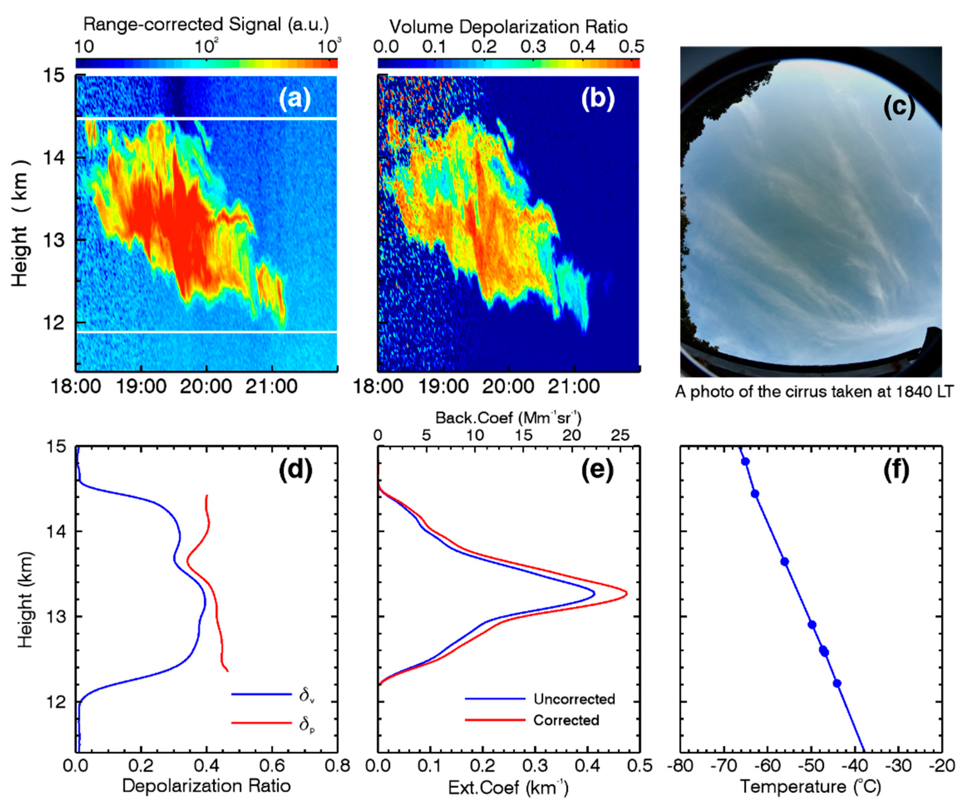
3.1. A Typical Cirrus Cloud Example

For a detailed study of the optical and geometrical properties of cirrus clouds, one measurement case observed by our polarization lidar which started at 1800 LT on 25 July 2019 and lasted for 190 min is presented in Figure 1. The time-height contour plots of range-corrected signal and volume depolarization ratio with 1 min and 30 m resolution are shown in Figure 1a,b. The cirrus cloud base and top height were 11.9 and 14.4 km respectively, yielding the mid-cloud height of 13.3 km. Figure 1c shows a photograph of the cirrus taken at 1840 LT, with a semitransparent, whitish cloud veil of smooth appearance, partly covering the sky. The time-average profiles of volume depolarization ratio (blue line) and particle depolarization ratio (red line) are presented in Figure 1d, note that only the particle depolarization ratio inside of the cirrus are provided. The mean values for volume depolarization ratio and particle depolarization ratio were 0.34 ± 0.04 and 0.41 ± 0.03 respectively. The time-average profile of extinction coefficient is presented in Figure 1e. The layer’s mean multiple scattering factor was 0.87 calculated by the model mentioned above, yielding the multiple scattering corrected COD and lidar ratio of 0.44 and 21.3 sr, respectively. The temperature profile shown in Figure 1f was provided by the radiosonde launched at 2000 LT, which revealed the cirrus base, top, and mid temperatures as −41.5, −64.2, and −52.9 °C, respectively.

In the analysis below, optical properties such as the COD, extinction coefficient, and lidar ratio are referred to as multiple scattering corrected ones, and the depolarization ratio is referred to as the particle depolarization ratio.

3.2. Frequency of Cirrus Occurrence

From March 2019 to February 2020, 228 days with a total of 3969 hours’ measurements were used for cirrus detection. A total of 168 cirrus layers were observed from 110 days, yielding an average frequency of cirrus occurrence, which was the ratio of days with cirrus present to the total days observed, which was 48% during the whole observation period. It should be noted that noon-time (1000 to 1400 LT) data were not included because of the poor signal-to-noise ratio at high altitude.

The monthly occurrence frequency of cirrus, and the monthly mean dust column mass density from MERRA-2 Model [45], which was calculated from daily values, are shown in Figure 2a. A clear seasonal cycle could be noticed. The frequency of cirrus occurrence showed a maximum value greater than 75% in June and July during the summer, and reached its minimum in winter (December to February) with a mean value of 24%. Dust column mass density, however, was largest during spring (March to May) with values larger than 1.0 × 10⁻⁴ kg/m³, followed by an abrupt drop in summer. The reason for the change was that dust which originated from the Taklimakan and Gobi Deserts was transported long-distance to Wuhan from the northwest mainly in the spring [46,47]. In summer, due to the move of the subtropical high to the north [48], Wuhan started to be dominated by warm and humid southern airflow, which inhibited the transport of Asian dust from the northwest. It was found that, except for the data for the summer months, the monthly cirrus occurrence frequency followed the same trend of the dust column mass density, with a positive correlation as shown in Figure 2b. This indicated that dust particles may be a dominant factor for cirrus formation in our site, suggesting a heterogeneous ice formation therein [49].

However, although the dust column mass density was less in summer, the cirrus occurrence frequency was the largest. This may be explained because cirrus clouds can be generated as outflowing ice crystals or the remains of the cirriform anvils of cumulonimbus associated with deep convection [10,50]. In summer, regional deep convective activities would frequently occur, thus produce more and frequent cirrus and transcend the influence of cirrus formation on dust particles.

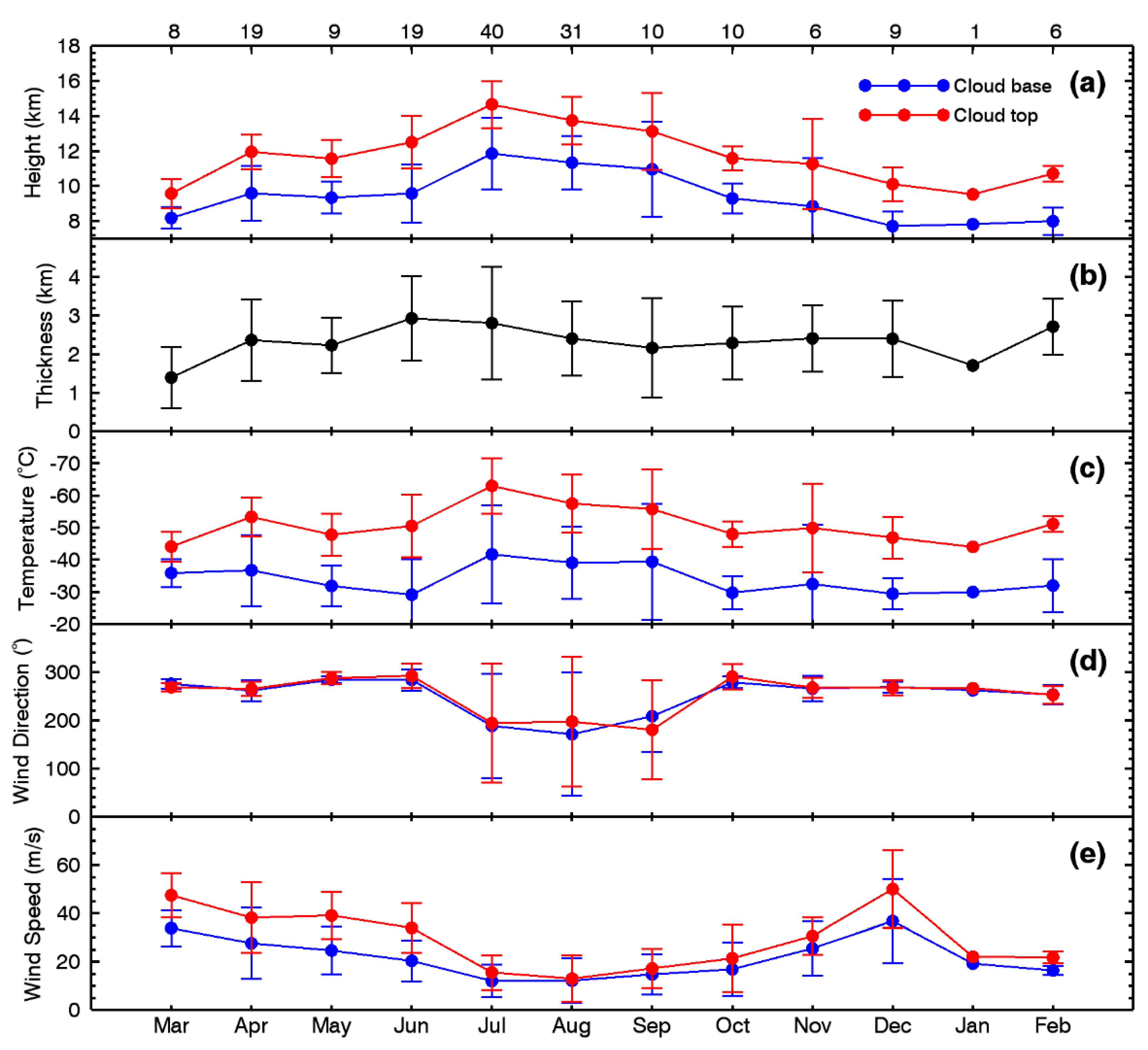
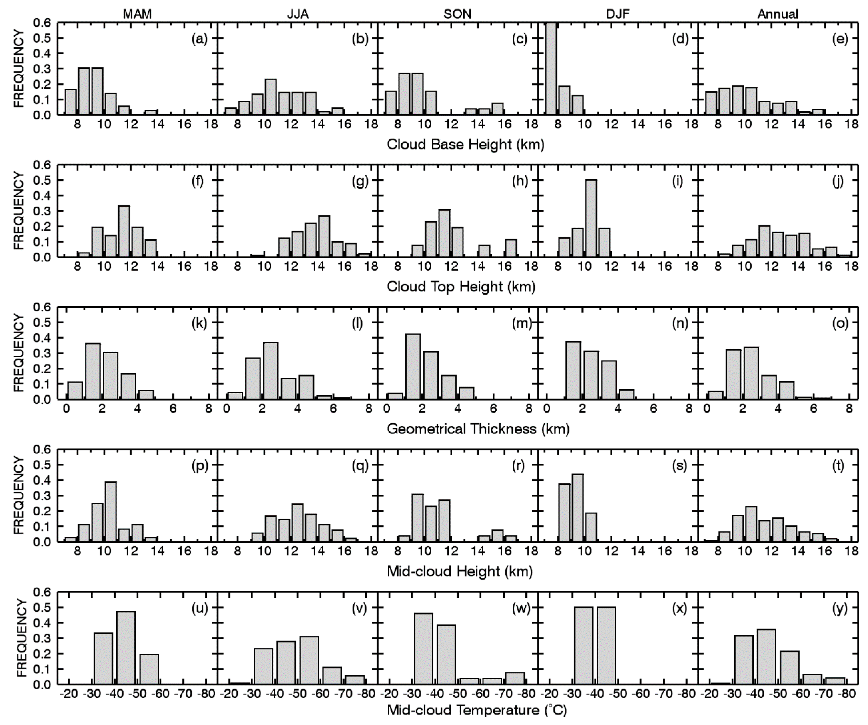
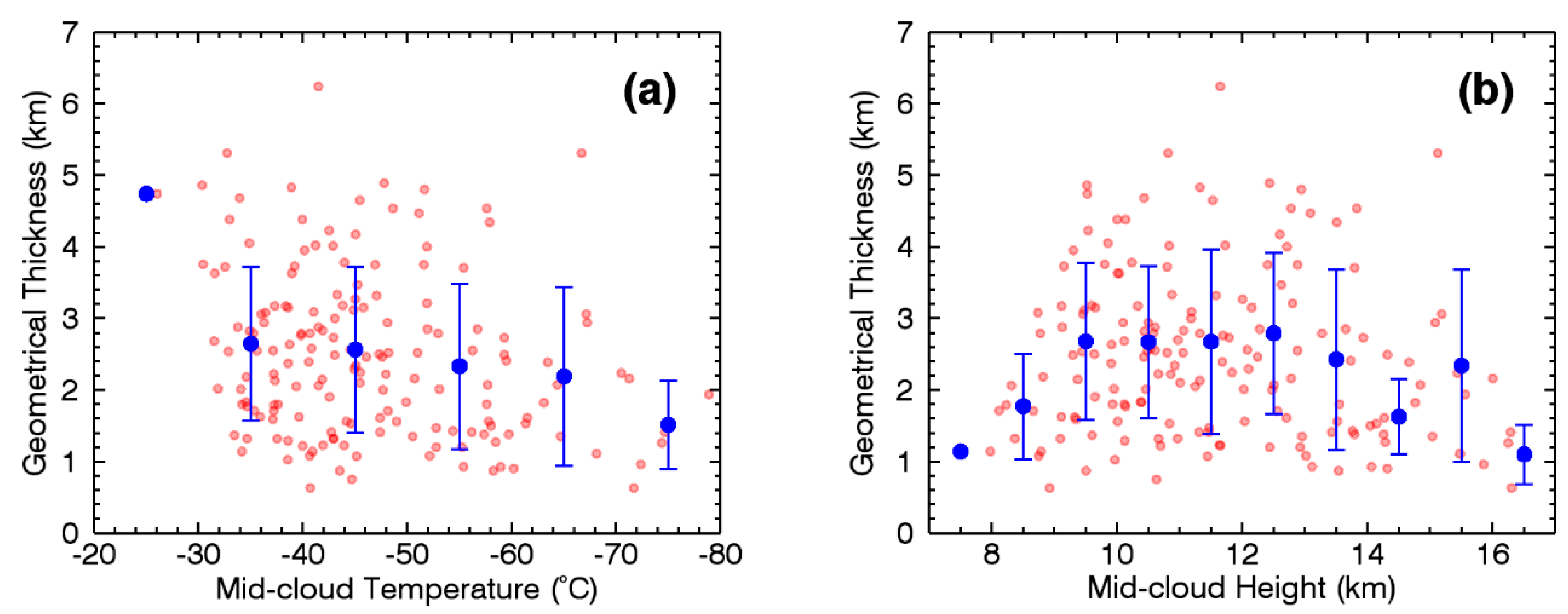
3.3. Geometrical and Meteorological Properties

Monthly-mean values of cirrus top and base heights, geometrical thickness, the corresponding mean temperature, wind direction, and speed magnitude at cloud base and top are presented in Figure 3. The cirrus top and base heights (temperatures) showed maximum (minimum) values in slightly–shifted summer months (July to September), while they reached minimum (maximum) values in winter (see Figure 3a,c). As for cirrus geometrical thickness, the variations were less obvious, but larger mean thickness values still occurred in the summer months (see Figure 3b). The wind directions shown in Figure 3d depict a distinct change from July to September with a southwesterly flow, while in other months, the winds were from the northwest. Additionally, wind speeds in these months reached their minimum with an average of about 12 m/s at cloud base and 15 m/s at cloud top (see Figure 3e). The distinct change of wind direction and wind speed should be the indicator of the arrival of the EASM.

Normalized histograms of cloud base and top heights, geometrical thickness, mid-cloud height, and mid-cloud temperature in terms of seasonal and annual statistics are shown in Figure 4. As Figure 4a–e shows, the cloud base height distribution was wider in summer and autumn (September to November) from 7 to 16 km, while most of the cirrus in spring (79%) and all the cirrus layers in winter had their cloud base height less than 10 km. Cirrus layers with cloud base height above 14 km only occurred in summer and autumn. As for cloud top height distribution (see Figure 4f–j), there was a peak at 14.5 km in summer, while the peak was around 11 km in other seasons. Cirrus clouds with cloud top height above 14 km were observed only in summer and autumn with a probability of 45% and 16% respectively. The distribution of geometrical thickness showed that there were more cirrus layers thicker than 4 km in summer with a probability of 18%, while the probability was about 7% in other seasons and showed little difference (see Figure 4k–o). Mid-cloud height distribution showed that cirrus in summer were obviously higher than that in other seasons. The probabilities of mid-cloud height larger than 11 km were 22% (spring), 77% (summer), 43% (autumn), 0 (winter), and 52% (annual), respectively (see Figure 4p–t). Figure 4u-v shows that the majority of the cirrus have the mid-cloud temperature fallen in the range between −30 to −60 °C. Cirrus with mid-cloud temperature less than −60 °C only occurred in summer and autumn with probabilities of 20% and 12%. Mean values of cirrus geometrical properties and corresponding temperatures from seasonal and annual statistics are summarized in

Table 1. Mean values and standard deviations (in parentheses) of cirrus geometrical properties and corresponding temperatures from seasonal and annual statistics.

	Cloud Base Height, km	Cloud Top Height, km	Geometrical Thickness, km	Mid-Cloud Height, km	Mid-Cloud Temperature, °C
MAM	9.2 (1.3)	11.3 (1.4)	2.1 (1.0)	10.4 (1.2)	−43.8 (6.4)
JJA	11.2 (2.0)	13.9 (1.6)	2.7 (1.2)	12.6 (1.7)	−49.0 (11.7)
SON	9.8 (2.3)	12.1 (2.0)	2.3 (1.0)	11.1 (2.0)	−44.5 (12.1)
DJF	7.8 (0.8)	10.3 (0.8)	2.5 (0.9)	9.2 (0.7)	−41.2 (5.4)
Annual	10.2 (2.2)	12.7 (2.0)	2.5 (1.1)	11.6 (2.0)	−46.4 (10.7)

.

Cirrus were more likely to occur at higher altitudes and have the largest mean values of cirrus base/top/mid heights in summer compared to that in other seasons, followed by autumn, and the least in winter. Additionally, cirrus in summer had the largest mean value of geometrical thickness. The reason was that from June to September (which included the summer months and part of autumn), the local convective activities were more frequent and intense because of the high surface temperature, together with the abundant water vapor supply from the Yangtze River and many lakes nearby, and a large amount of upper tropospheric water vapor induced by the EASM from Indochina Peninsula and the South China Sea [51,52]. These convective activities produced cumulonimbus clouds which could reach a higher altitude with a large vertical scale. Cirrus formed by these cumulonimbus clouds could occur at high altitude and with large geometrical thickness. On the other hand, in situ formations of cirrus by supersaturation promoted by mesoscale uplift [53] with mid-cloud height larger than ~14km, which mainly occurred in summer, would also contribute to larger mean values of cloud base/top/mid-cloud height. A more detailed discussion of these two cirrus formation mechanisms will be presented in Section 4.

The dependence of cirrus geometrical thickness and mid-cloud temperature based on all cirrus events is presented in Figure 5a. Cirrus geometrical thickness tended to decrease with the lowering mid-cloud temperature. The maximum mean value of thickness (grouped in 10 °C intervals) was 2.6 km observed at ~−35 °C. Referring to other studies, Giannakaki et al. [19] observed a maximum thickness of ~3.5 km at −47.5 °C at Thessaloniki (40.6°N, 22.9°E). Platt et al. [54] showed a peak of cirrus thickness in the −30 °C to −40 °C range for mid-latitude cirrus and −55 °C to −70 °C for tropical cirrus. Sunilkumar et al. [55] observed cloud thickness of ~1.7 km for temperatures between −55 °C to −70 °C of tropical cirrus. It could be concluded that cirrus in middle and high latitudes were generally warmer and thicker than those over the tropics.

The relationship between cirrus geometrical thickness and mid-cloud height is presented in Figure 5b. Mean cloud thickness of ~2.7 km was observed at a mid-cloud height between 9 to 13 km, and decreased to ~1.5 km for clouds higher than 13 km or lower than 9 km. It had to be noted that the point of mid-cloud temperature higher than -30 °C and the point of mid-cloud height lower than 8 km were not taken into consideration here because of low statistical significance since it referred to only one measurement.

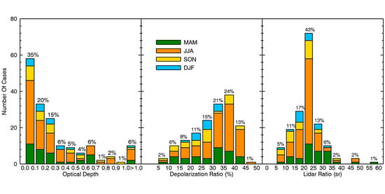
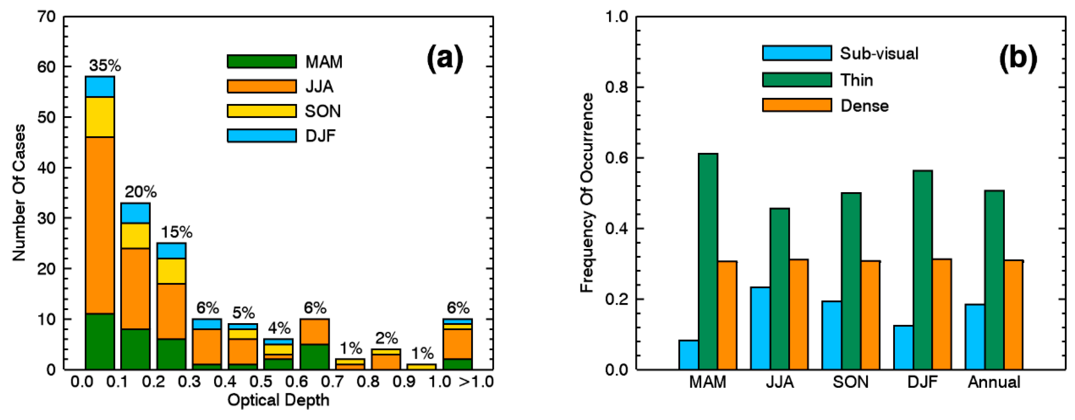
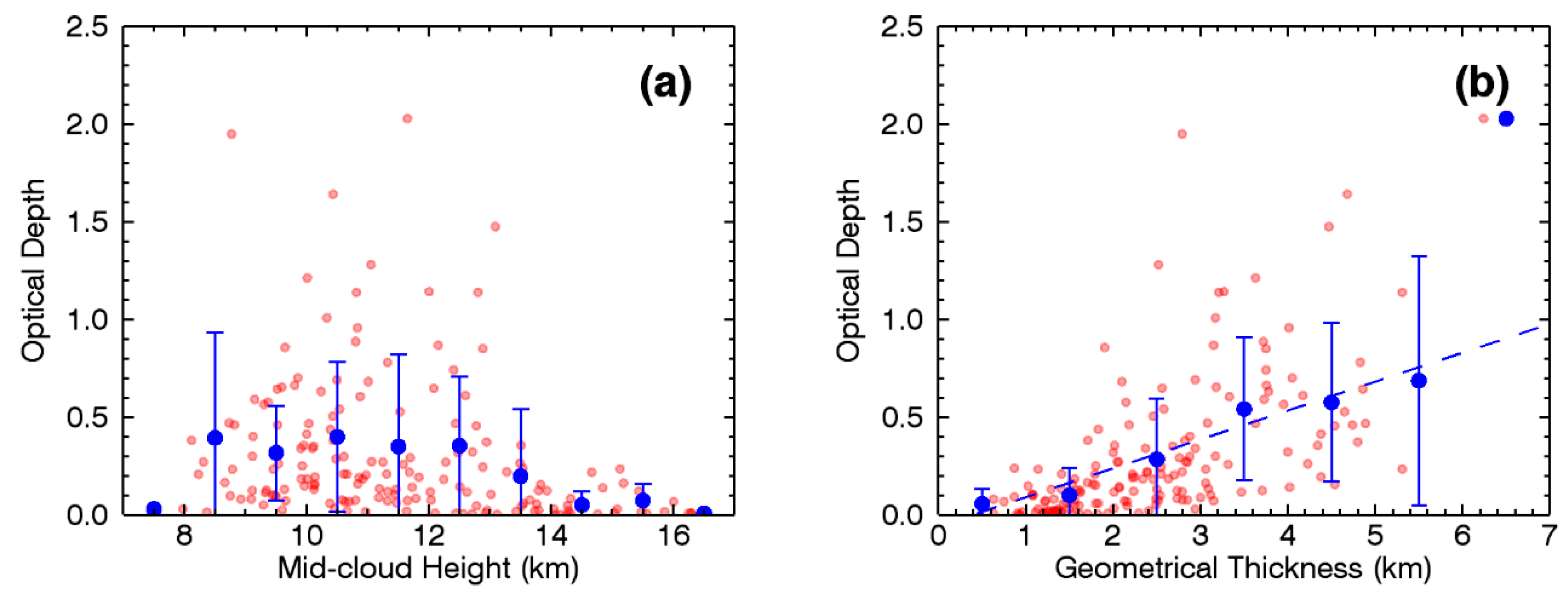
3.4. Optical Properties

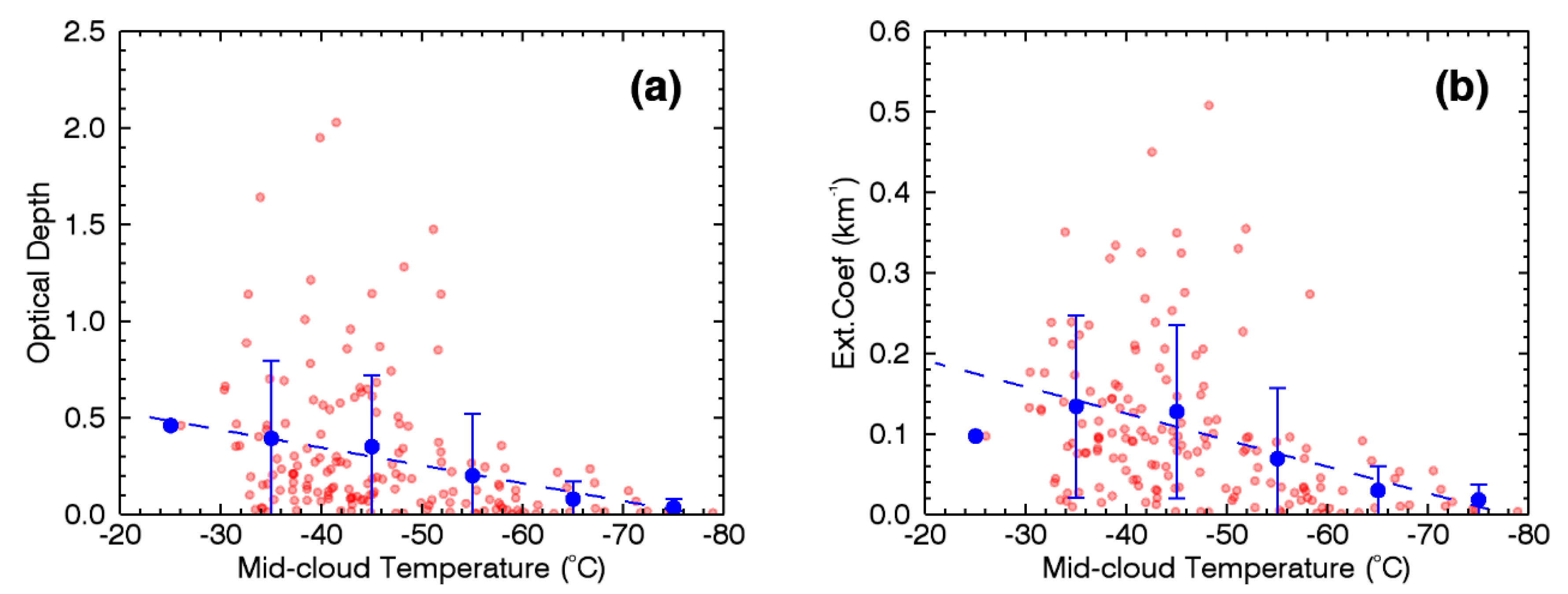
3.4.1. Optical Depth

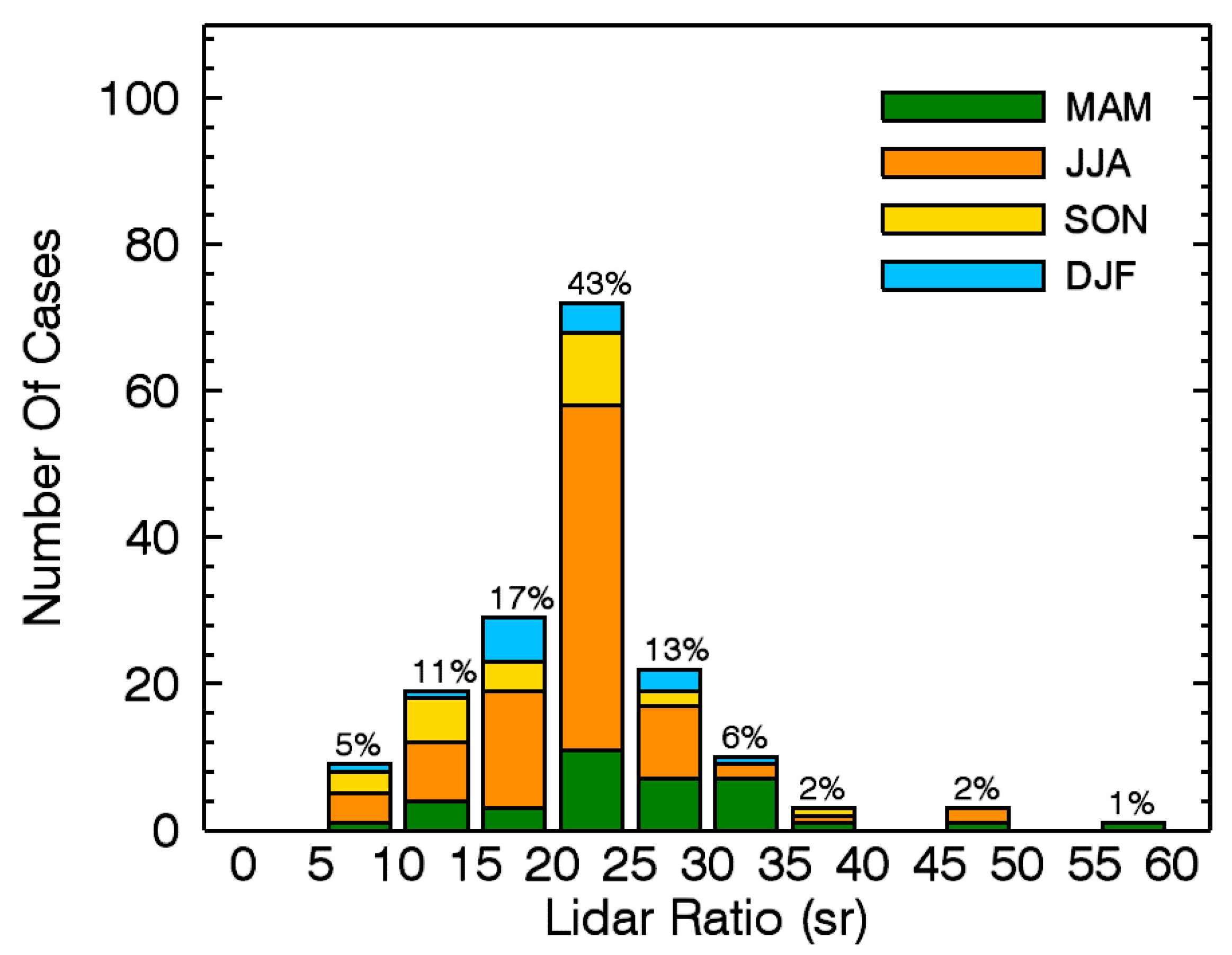
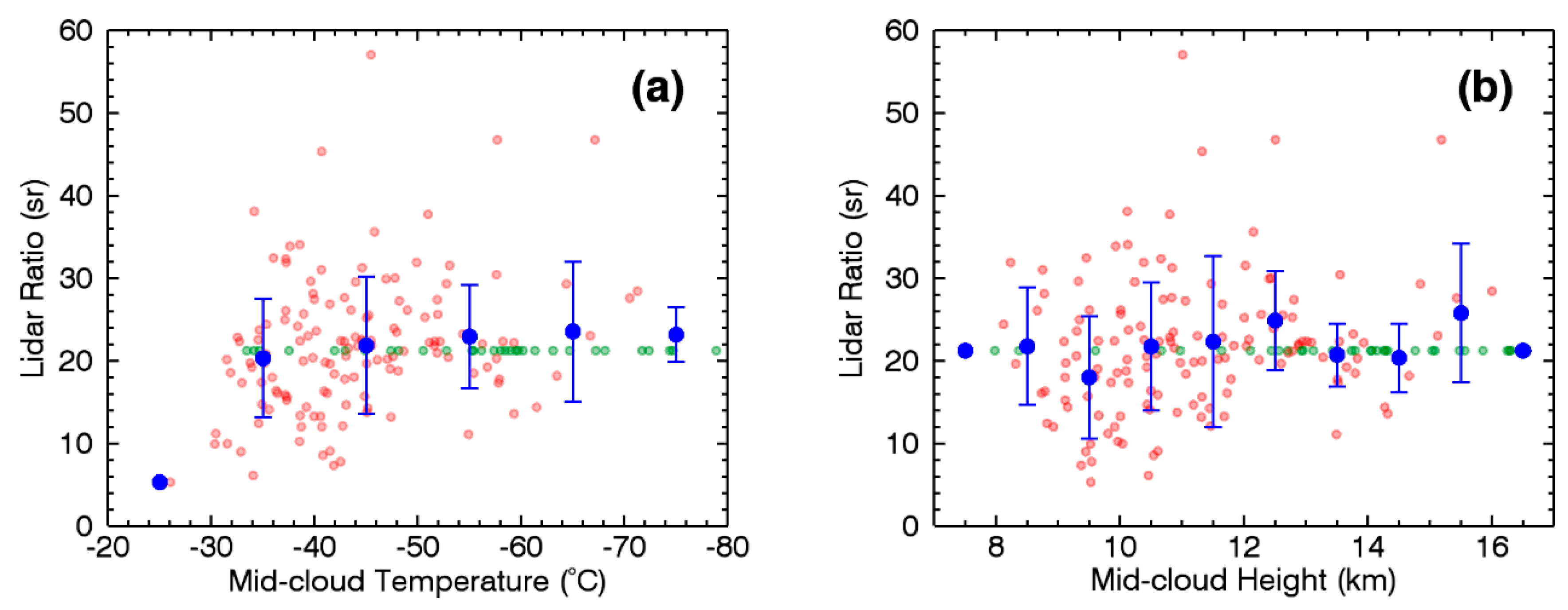
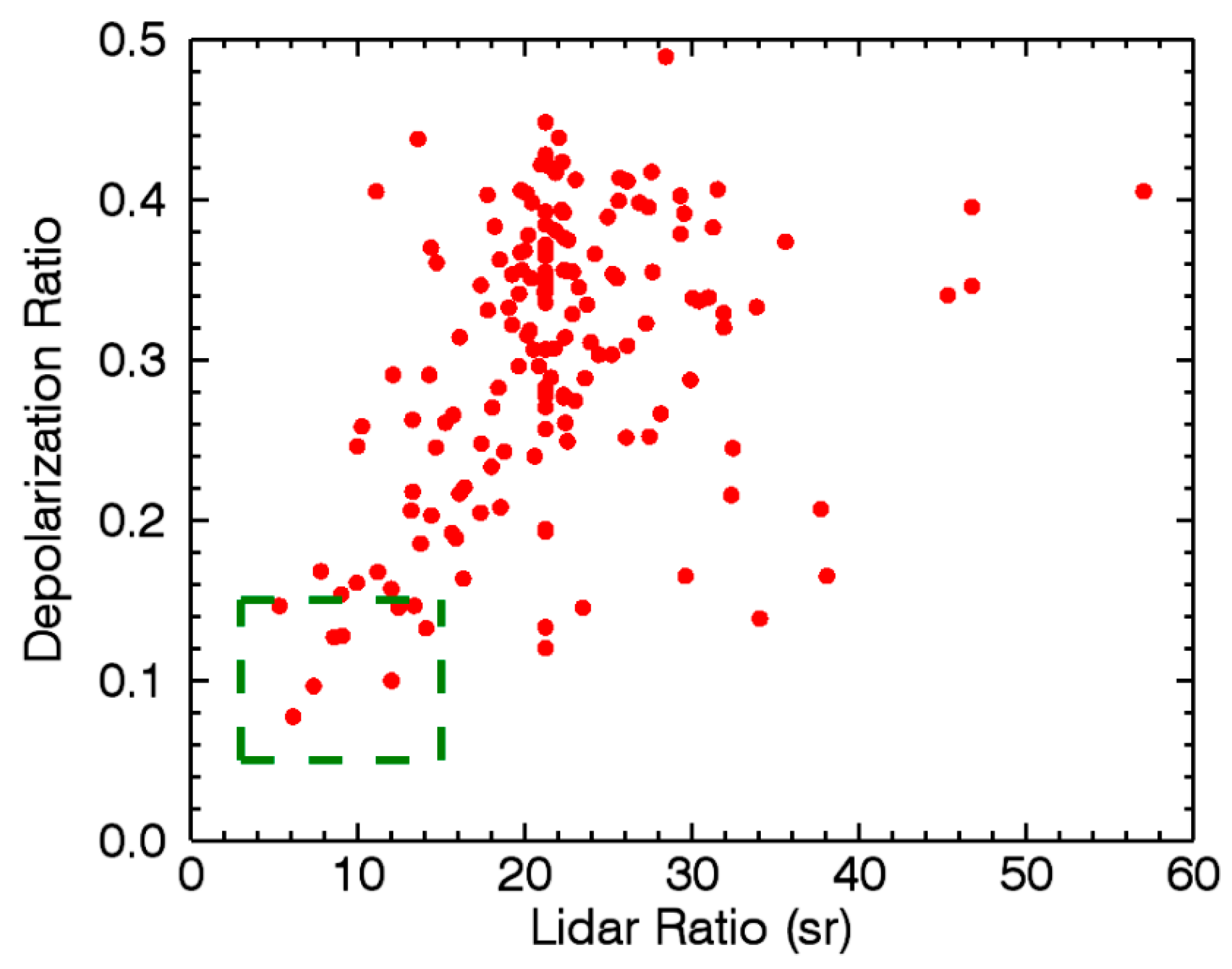
According to our results, the COD had a broad range from 0.001 to 2.02 of all cirrus events. The most prevalent region of the COD was below 0.1 with a percentage of 35% (see Figure 6a). 70% of all layers had a COD less than 0.3. The trend that most cirrus clouds have a smaller COD was applicable for all seasons. Cirrus clouds in summer had the most widespread COD while nearly all cirrus clouds in winter had a COD less than 0.6. A total of 10 cirrus layers had a COD larger than 1.0, of which 6 of them were from summer. The seasonal mean CODs were 0.30 ± 0.31 (spring), 0.29 ± 0.29 (summer), 0.30 ± 0.31 (autumn), and 0.33 ± 0.46 (winter), respectively, which did not show an obvious seasonal cycle.

Cirrus can be classified as sub-visual (COD < 0.03), thin (0.03 < COD < 0.3), and dense (COD > 0.3) according to Sassen and Cho [56]. The seasonal and annual frequency of occurrence of different cirrus categories is presented in Figure 6b. Thin cirrus clouds occurred most frequently while sub-visual cirrus the least for all seasons. Sub-visual cirrus clouds had the highest (lowest) fraction in summer (spring), while thin cirrus had the highest (lowest) fraction in spring (summer). The fraction for dense cirrus remained the same for all seasons. The detailed values are summarized in

Table 2. Mean values and standard deviations (in parentheses) of cirrus optical properties from seasonal and annual statistics.

	Optical Depth	SBV/Thin/Dense (%)	Extinction Coefficient, km−1	Lidar Ratio, sr	Depolarization Ratio
MAM	0.30 (0.31)	8/61/31	0.13 (0.10)	25.4 (9.6)	0.29 (0.10)
JJA	0.29 (0.39)	23/46/31	0.09 (0.09)	21.2 (6.4)	0.33 (0.08)
SON	0.30 (0.31)	19/50/31	0.12 (0.11)	18.9 (7.0)	0.26 (0.10)
DJF	0.33 (0.46)	13/56/31	0.13 (0.16)	20.4 (6.0)	0.26 (0.05)
Annual	0.30 (0.36)	18/51/31	0.11 (0.11)	21.6 (7.5)	0.30 (0.09)

.

The relationship between the COD and mid-cloud height is presented in Figure 7a. The COD was larger for cirrus clouds with a mid-cloud height range between 8 and 13 km and with a mean value of 0.36 ± 0.38, followed by a rapid decrease for mid-cloud height larger than 14 km. The mean COD for cirrus clouds higher than 14 km was 0.05 ± 0.07. A similar trend that the COD decreased at higher cloud height was also found by Lakkis et al. [28], Wang et al. [57], and Das et al. [58].

The relation between the COD and geometrical thickness is presented in Figure 7b. Excluding the point of geometrical thickness above 6 km (which was of low statistical significance since it referred to only one measurement), a positive linear relation of the COD and geometrical thickness was found. The linear relationship was also reported by other researchers [19,28,57,59].

The low values of the COD (shown in Figure 7a) and geometrical thickness (shown in Figure 5b) at high altitude, especially at mid-cloud height larger than 14 km, may be due to the different cirrus formation mechanism compared to those at a lower altitude. A detailed discussion will be presented in Section 4.

The dependence of the COD and layer-mean extinction coefficient (ratio of COD to geometrical thickness) to mid-cloud temperature are shown in Figure 8. Both of them tended to decrease with the lowering mid-cloud temperature, which was in agreement with other studies [8,19,55,58,59]. Moreover, Sassen et al. [60] found a linear relationship between mid-cloud temperature and the COD as well as the extinction coefficient for mid-latitude cirrus, while Sunilkumar et al. [55] suggested a second-order polynomial function for tropical cirrus. Here we applied linear functional forms as $\mathsf{\tau }$= 0.712 + 0.009 T and $\mathsf{\sigma }$ = 0.257 + 0.0033 T ($\mathsf{\tau }$ for COD, $\mathsf{\sigma }$ for mean extinction coefficient and T for mid-cloud temperature in °C). The results are shown by the dashed line in Figure 8.

3.4.2. Lidar Ratio

The lidar ratio was closely linked to ice crystal sizes and shapes [61]. Sassen et al. [62] simulated simple hexagonal ice crystals and found the lidar ratio of 38.5 sr for thin-plate, 11.6 sr for thick-plate, and 26.3 sr for column shape ice crystals. Reichardt et al. [63] used ray-tracing calculations and found the lidar ratio was sensitive to particle-shape distortions, which was the deviation from the ideal hexagonal structure (pristine ice particles). Generally, an increase in shape distortion leads to a higher lidar ratio. Seifert et al. [7] found that the lidar ratio for larger, more complex ice crystals tended to show a higher degree of distortion than small ice crystals. Laboratory experiments and in situ particle sampling have indicated that temperature is one of the principal factors that control ice crystal shape thus affecting the cirrus lidar ratio [64,65].

Figure 9 shows the histogram of the cirrus lidar ratio in every 5 sr interval with seasonal proportion. The lidar ratio had a wide range from 5.3 to 57.0 sr, distributed primarily in 5–40 sr, and peaked at ~22.5 sr. It should be noted that the lidar ratio of sub-visual cirrus, which cannot be determined by the Klett-Fernald method was set as ~21 sr manually. When sub-visual cirrus cases were excluded, the percentage of the lidar ratio range between 20 and 25 sr was 24%, which was still the peak of the distribution. As for seasonal variance, the most prevalent value for winter cirrus was between 15 and 20 sr, while in other seasons it fell to a range between 20 and 25 sr.

The seasonal mean values of the lidar ratio were 25.4 ± 9.6 (spring), 21.2 ± 6.4 (summer), 18.9 ± 7.0 (autumn), and 20.4 ± 6.0 (winter), respectively. The larger value in spring may be due to the influence of dust, which reached its maximum amount in spring as Figure 2a shows. Heterogeneous ice nucleation caused by dust particles would lead to a growth in crystal sizes [66], thus resulting in a relatively larger lidar ratio.

The relationships between the lidar ratio and mid-cloud temperature and mid-cloud height are shown in Figure 10. No clear dependence was found on mid-cloud temperature (shown in Figure 10a) and mid-cloud height (shown in Figure 10b).

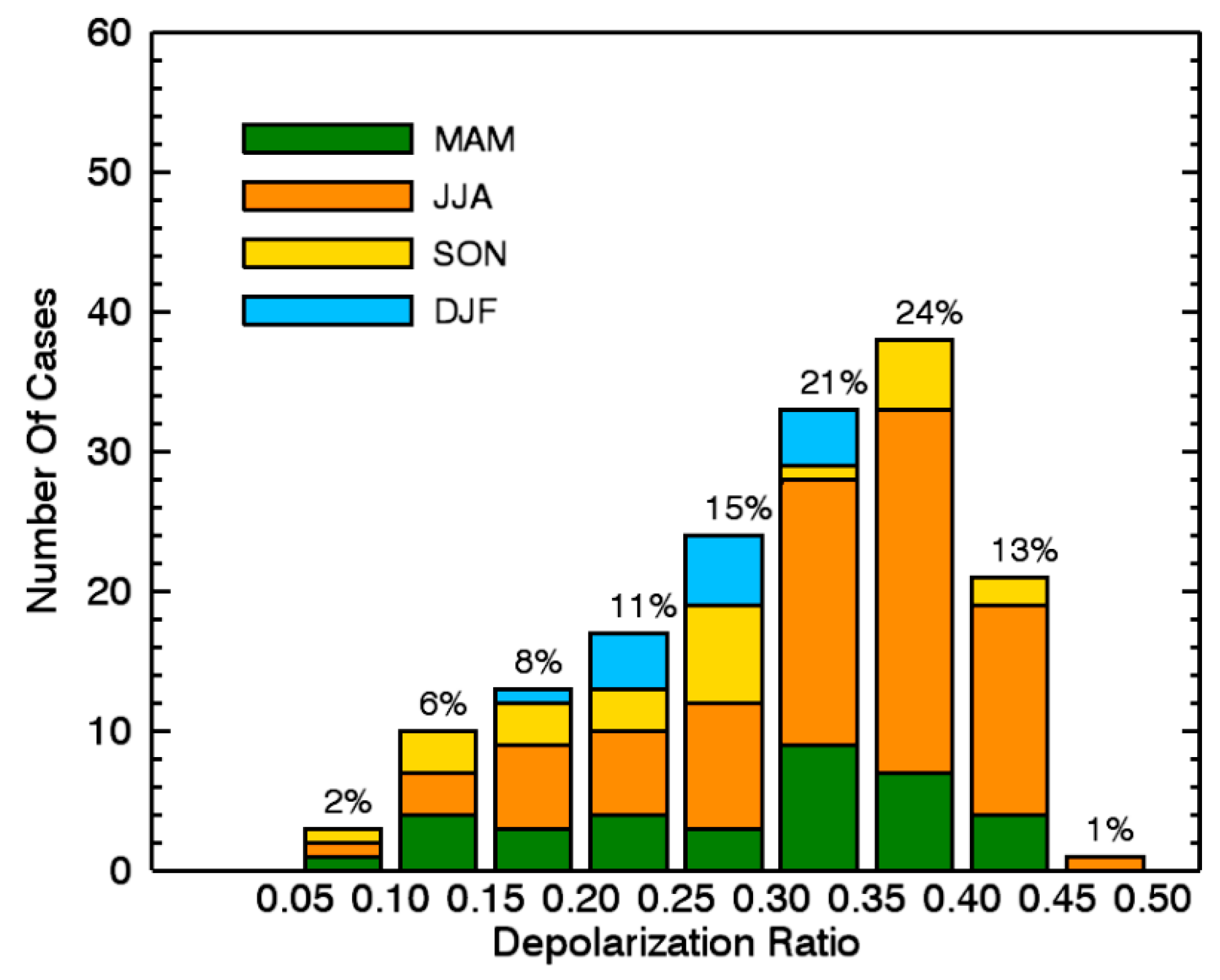
3.4.3. Depolarization Ratio

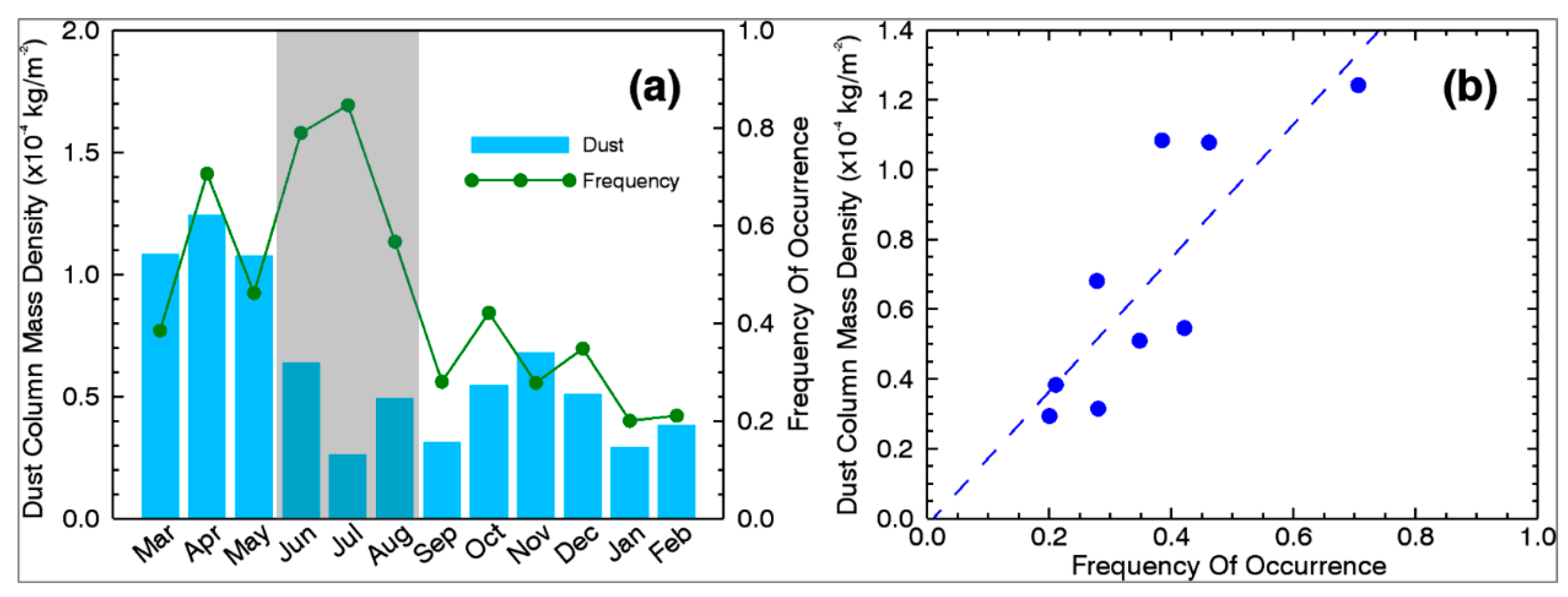
The depolarization ratio was sensitive to crystal shape, especially aspect ratios [67]. Noel et al. [68] classified ice crystals into three shape groups. Low values of depolarization ratio less than 0.25 were attributed to thin plate-like particles (aspect ratio < 0.1). High values of depolarization ratio > 0.5 were found to be the signature of column-like particles (aspect ratio > 1.5) and crystals of high complexity, such as bullet rosettes. Irregular particle shapes (aspect ratio ~1.0) produced a depolarization ratio ranging from 0.25 to 0.5. They also pointed out that particles close to sphericity, which are in the early stage of ice formation or through the riming process, would also produce low polarization values. The shape of ice particles was highly sensitive to temperature and their relations have been well analyzed in former studies. In general, smaller size and larger aspect ratio ice crystals with a larger depolarization ratio, preferred a lower temperature and were found in higher cirrus clouds [61,67,68].

A histogram of cirrus particle depolarization ratio with seasonal proportion is shown in Figure 11. The depolarization ratio ranged from 0.07 to 0.49, with the most frequently observed values between 0.3 and 0.4, indicating that these cirrus clouds were mostly composed of ice crystals of irregular shapes. For seasonal variation, cirrus in autumn and winter preferred smaller values and were most frequently observed between 0.2 and 0.3, while in spring and summer they were most frequently observed between 0.3 and 0.4. Values of mean depolarization ratio for different seasons were 0.29 ± 0.10 (spring), 0.33 ± 0.08 (summer), 0.26 ± 0.10 (autumn), and 0.26 ± 0.05 (winter), respectively. The higher value in summer was due to the larger percentage of cirrus at higher altitudes thus a lower ambient temperature. Ice crystals in low temperatures were more likely to have a large aspect ratio thus a large depolarization ratio [68].

In Figure 12, the dependences of the depolarization ratio on mid-cloud temperature and mid-cloud height are presented. Excluding the points of mid-cloud temperature higher than −30 °C (shown in Figure 12a) and mid-cloud height below 8 km and above 16 km (shown in Figure 12b), which was of low statistical significance since they were referred to in one or two cases, the depolarization ratio tended to increase with the lowering mid-cloud temperature and increasing mid-cloud height, as expected. The reason for this trend was that as the cloud height increased and the temperature dropped, the irregular shape crystals with smaller size and greater aspect ratio were formed, which resulted in the enhancement of the depolarization ratio. Additionally, the depolarization ratio was found to be more sensitive to mid-cloud temperature (mid-cloud height) in warmer (lower) cirrus clouds, which was in accordance with the findings by Dai et al. [8]. This indicated that ice crystal shapes may be more stable with decreasing temperature in a colder environment.

As the depolarization ratio and lidar ratio were both connected to the ice crystal shape, their relationship was further examined as shown in Figure 13. The depolarization ratio tended to increase with the increasing lidar ratio for a lidar ratio value less than 30 sr. For larger lidar ratios, the cirrus event number was not sufficient enough to deliver a clear relationship.

Horizontally-oriented ice crystals produced a near-zero depolarization ratio and low lidar ratio values ~3 sr when detected by a vertically pointed lidar beam [69,70]. However, only falling ice crystals with a planar shape (except for Parry arc, which is rarely observed and not considered in this paper [71]) and large size (>100–200 mm, depending on shape [72]) can bring this effect [69,73], which was more likely to be generated at a relatively higher temperature [68]. Cirrus that contain horizontally-oriented ice crystals, which could be determined by those with low values of both depolarization ratio and lidar ratio, are marked by a green rectangle in Figure 13. All these layers were located at altitudes less than 10.5 km (for mid-cloud height) and a mid-cloud temperature higher than −42 °C.

4. Discussion

Cirrus can be formed by the outflow or remains of cirriform anvils of cumulonimbi associated with deep convection, which is common in tropical and subtropical areas [13,74]. Such cirrus clouds appear as rather opaque, textured clouds with irregular boundaries [7].

Cirrus clouds can also be generated due to homogeneous freezing by a slow, synoptic-scale uplift of a humid layer at a higher altitude, where the ambient temperature is low [75]. Cirrus induced by these processes usually appear as rather tenuous, laminar layers of low COD spreading over large areas [7]. These kinds of cirrus clouds are usually found in a mid-latitude region [76,77] and are also common in tropical areas [7,13].

In Wuhan, both types of cirrus can be observed. The broad distribution of the COD and geometrical thickness for cirrus with a mid-cloud height lower than 14 km (see Figure 5b and Figure 7a), can be evidence that these cirrus clouds are formed from cumulonimbus cloud due to deep convection. However, cirrus with a mid-cloud height larger than 14 km are more likely to be formed by the other mechanism. These cirrus clouds have their COD and geometrical thickness trapped in a limited range (COD < 0.3, geometrical thickness < ~2.5 km) with a small mean value (0.05 ± 0.07 for COD, 1.8 ± 1.0 for geometrical thickness). Additionally, these clouds only occur in summer and autumn (as shown in Figure 4), when water vapor is abundant in the upper troposphere, together with a low ambient temperature, which are the two key elements for the second formation mechanism [74,78]. Moreover, Liu and Zipser [79] showed that only 1.38% of convective systems, and consequently their generated cirrus clouds, could reach 14 km of altitude.

According to our observations, the annual mean values for cloud base height is 10.2 ± 2.2 km, for cloud top height, 12.7 ± 2.0 km, and for cloud geometrical thickness, 2.5 ± 1.1 km. These values are similar to those reported by Lakkis et al. [80] for Buenos Aires (34.6°S, 58.5°W): 9.63 ± 0.92 (base height), 11.82 ± 0.86 (top height), 2.41 ± 0.95 (thickness). Gouveia et al. [13] reported for cirrus in Amazonia (2.89°S, 59.97°W) a base and top height of 12.9 ± 2.2 km and 14.3 ± 1.9 km, while Sassen et al. [31,69] showed mean values of 8.8 and 11.2 for cirrus base and top height respectively at Salt Lake City (40.8°N, 111.8°W). Some cirrus characteristics reported around the world are summarized in

Table 3. Cirrus cloud statistical characteristics from long-term (at least a few months) ground-based lidar measurements at different locations around the world.

Location	Measurement Period	Wave-Length (nm)	CBH 1 (km)	CTH 2 (km)	GT 3 (km)	Temperature (℃)	COD	SBV/Thin/Dense 4 (%)	Lidar Ratio (sr)	Depolarization Ratio
Kuopio [81] 62.74°N, 27.54°E	Nov. 2012–2019	355/532/1064	8.6 ± 1.1	9.8 ± 1.1	1.2 ± 0.7	−43 ± 10 (base) −57 ± 9 (top) 5	0.24 ± 0.20	3/71/26	31 ± 7	0.38 ± 0.07
Thessaloniki [19] 40.6°N, 22.9°E	2000–2006	355/532	9.0 ±1.1	11.7 ± 0.9	2.7 ± 0.9	−52 (mid) 6	0.31 ± 0.24	3/57/40	30 ± 17
Salt Lake City [31,69] 40.8°N, 111.8°W	1986-1996	694	8.8	11.2	1.81	−34 (base) −54 (top)	-	16/35/48	24 ± 38	0.33 ± 0.11
Seoul [82] 37.5°N, 127. 0°E	Jul. 2006–Jun. 2009	532/1064	8.8 ± 1.4	10.6 ± 1.2	-	-	0.42 ± 0.40	50 (<0.3)	25 (assumption)	0.30 ± 0.06
COVE [83] 37°N, 76°W	2006–2008	532/1064	9.8 ± 1.8	11.6 ± 1.6	1.85 ± 0.97	-	-	10/50/40	-	-
Wuhan (this study) 30.5°N, 114.4°E	Mar.2019– Feb.2020	532	10.2 ± 2.2	12.7 ± 2.0	2.5 ± 1.1	−46 ± 11 (mid)	0.30 ± 0.36	18/51/31	21.6 ± 7.5	0.30 ± 0.09
Gwal Pahari [81] 28.43°N, 77.15°E	Mar. 2008–Mar. 2009	355/532/1064	9.0 ± 1.6	10.6 ± 1.8	1.5 ± 0.7	−33 ± 6 (base) −45 ± 4 (top)	0.45 ± 0.30	0/20/80	28 ± 22	-
Chung-Li [84] 24.58°N,121.10°E	1999–2006	532	12.3 ± 2.2	14.4 ± 1.9	2.08 ± 1.2	-	0.16 ± 0.27	38/47/15	23 ± 16	0.2 (peak occurrence)
Gadanki [85] 13.5°N, 79.2°E	1998–2013	532	13.0 ± 2.2	15.3 ± 2.0	2.3 ± 1.3	−65 ± 12 (mid)	-	52/36/11	25 (assumption)	-
Hulule [7] 4.1°N, 73.3°E,	1999, 2000	532	11.9 ±1.6	11.9 ± 1.6	1.8 ± 1.0	−58 ± 11 (mid)	0.28 ± 0.29	15/49/36	32 ± 10	-
Amazonia [13] 2.89°S, 59.97°W	Jul. 2011–Jun. 2012	355	12.9 ± 2.2	14.3 ± 1.9	1.4 ± 1.1	−60 ± 15 (max. back) 7	0.25 ± 0.46	41.6/37.8/20.5	23.3 ± 8.0	-

¹ CBH = cloud base height. ² CTH = cloud base height. ³ GT = geometrical thickness. ⁴ SBV = sub-visual cirrus, Thin = optically thin cirrus, Dense = optically dense cirrus. ⁵ base = temperature at cloud base, top = temperature at cloud top. ⁶ mid = mid-cloud temperature. ⁷ temperature at the maximum of backscattering coefficient.

for comparison. It can be concluded that cirrus in the tropics are generally higher than those at mid latitudes or even higher latitudes.

The annual percentages of sub-visual, thin, and dense cirrus are 18%, 51%, and 31%, respectively. These values are very similar to those reported by Seifert et al. [7] observed for Hulule (4.1°N, 73.3°E): 15% (sub-visual), 49% (thin), and 36% (dense). However, other studies of tropical and subtropical cirrus show a larger percentage of sub-visual ones, yielding the distribution of 41.6%, 37.8%, and 20.5% at Amazonia (2.89°S, 59.97°W) [13], 52%, 36%, and 11% at Gadanki (13.5°N, 79.2°E) [85] for sub-visual, thin and dense cirrus, respectively. Observations by Sassen and Campbell [31] for mid-latitude cirrus at Salt Lake City (40.8°N, 111.8°W) showed a percentage of 16% (sub-visual), 35% (thin), and 48% (dense).

The annual mean COD is 0.30 ± 0.36, which is similar to the mean values of 0.31 ± 0.24 reported by Giannakaki et al. [19] at Thessaloniki (40.6°N, 22.9°E) and 0.30 ± 0.30 reported by Voudouri et al. [81] at Elandsfontein (26.25°S, 29.43°E). However, the mean value found in this study is significantly larger than the value of 0.16 ± 0.27 reported by Das et al. [58] at Chung-Li (24.58°N, 121.10°E) and slightly less than the value of 0.42 ± 0.40 reported by Kim et al. [82] at Seoul (37.5°N, 127. 0°E).

By comparing the results obtained in different sites globally, the occurrence of dense cirrus in mid latitudes is clearly enhanced compared with that in the subtropics and tropics, thus yielding a larger mean COD value.

The annual mean lidar ratio is 21.6 ± 7.5 sr. Observations at other sites show that the lidar ratio varies greatly from ~10 to 33 sr. The typical values are ~20 to 25 sr for tropical and subtropical areas [13,58,81,86], and ~30 sr for mid latitudes [19,81,87]. The reason for the latitudinal variation may be explained by the difference in the dominant cirrus formation mechanism mentioned above, which results in different crystal shapes. In the tropics, most of the cirrus are associated with convection systems [88]. Stronger convection may initiate the formation of a larger number of crystals that then show a smaller mean size and more simple forms with regular structures (hexagonal columns and plates), which show a small lidar ratio [7].

The mean annual depolarization ratio is 0.30 ± 0.09. For other observation sites, the mean depolarization ratio of cirrus is 0.30 ± 0.06 at Seoul (37.5°N, 127. 0°E) [82], 0.33 ± 0.11 at Salt Lake City (40.8°N, 111.8°W) [69] and 0.38 ± 0.07 at Kuopio (62.74°N, 27.54°E) [81]. The increasing depolarization values with increasing latitude may indicate the change of dominating crystal shapes of cirrus at different latitudes.

It has to be noted that the measurement sensitivities are relevant to the laser wavelength and energy of the lidar. The most widely used laser wavelengths for aerosol and cloud measurements are 355 nm, 532 nm, and 1064 nm nowadays. However, as backscatter of molecules (Rayleigh scattering) is inversely proportional to the fourth power of the wavelength, lidars with shorter working wavelengths suffer from a larger impact of Rayleigh scattering, which makes them less suitable for sub-visual cirrus detection. Lasers of 532 nm and 1064 nm are capable of detecting very thin cirrus layers (with COD as small as 0.0001) when the laser energy is strong enough. If the laser energy is weak, the small signal-to-noise ratio may influence the detection of thin cirrus at a high altitude, too.

5. Concluding Remarks

The geometrical/optical properties and seasonal variations of cirrus clouds over a 30°N plain area were obtained from ground-based polarization lidar measurements between March 2019 and February 2020 at Wuhan (30.5°N, 114.4°E), China. A total of 168 cirrus events were identified from ~3969 h worth of lidar data on 228 different days with an overall occurrence frequency of 48%. These cirrus clouds appeared at heights from ~7 to 17 km above ground level where the ambient temperature was between −26 °C and −79 °C. The cirrus geometrical thickness tended to decrease with decreasing temperature. Mean values of their cloud base, cloud top, mid-cloud height, and mid-cloud temperature were 10.2 ± 2.2 km, 12.7 ± 2.0 km, 11.6 ± 2.0 km, and −46.4 ± 10.7 °C respectively.

The cirrus optical properties were determined by taking account of the multiple scattering correction. The COD ranged from 0.001 to 2.02 with a mean of 0.30 ± 0.36, while the layer-mean extinction coefficient varied from 7 × 10⁻⁴ to 0.70 km⁻¹ with a mean of 0.11 ± 0.11 km⁻¹. In terms of the magnitude of the COD, the sub-visual, thin, and dense cirrus clouds accounted respectively for 18%, 51%, and 31% of the total of the observed cirrus events. There was a positive correlation between the COD and cirrus geometrical thickness. The cirrus clouds had the lidar ratio between 5.3 and 57.0 sr (a mean of 21.6 ± 7.5 sr) and particle depolarization ratio varying from 0.07 to 0.49 (a mean of 0.30 ± 0.09). There existed a positive correlation, with the correlation coefficient of 0.56, between the particle depolarization ratio and lidar ratio for the lidar ratio value being less than 30 sr.

At the 30°N plain site, the observed cirrus clouds showed some seasonal dependence with the cloud altitude maximizing in a slightly-shifted summertime (July to September) where the southwesterly wind prevailed and minimizing in winter months. In addition, a positive correlation between the cirrus occurrence frequency and dust column mass density was found in other seasons except for summer, suggesting a heterogeneous ice formation therein. The seasonally-averaged cirrus lidar ratio showed the maximum value in spring when the dust column mass density was the largest. The depolarization ratio maximized in summer and showed similar values in other seasons. However, the seasonally-averaged cirrus optical depth appeared to be independent of seasons.

References

1. Liou, K.-N. Influence of Cirrus Clouds on Weather and Climate Processes: A Global Perspective. Mon. Weather Rev. 1986, 114, 1167. [Google Scholar] [CrossRef]
2. Nazaryan, H.; McCormick, M.P.; Menzel, W.P. Global characterization of cirrus clouds using CALIPSO data. J. Geophys. Res. Atmos. 2008, 113. [Google Scholar] [CrossRef]
3. Campbell, J.R.; Lolli, S.; Lewis, J.R.; Gu, Y.; Welton, E.J. Daytime Cirrus Cloud Top-of-the-Atmosphere Radiative Forcing Properties at a Midlatitude Site and Their Global Consequences. J. Appl. Meteorol. Climatol. 2016, 55, 1667–1679. [Google Scholar] [CrossRef]
4. Solomon, S.; Qin, D.; Manning, M.; Chen, Z.; Marquis, M.; Averyt, K.; Tignor, M.; Miller, H. IPCC, 2007: Climate change 2007: The physical science basis. In Contribution of Working Group I to the Fourth Assessment Report of the Intergovernmental Panel on Climate Change; Cambridge University Press: Cambridge, UK; New York, NY, USA, 2007. [Google Scholar] [CrossRef]
5. Fu, Q.; Liou, K.N. Parameterization of the Radiative Properties of Cirrus Clouds. J. Atmos. Sci. 1993, 50, 2008–2025. [Google Scholar] [CrossRef] [Green Version]
6. Zerefos, C.S.; Eleftheratos, K.; Balis, D.S.; Zanis, P.; Tselioudis, G.; Meleti, C. Evidence of impact of aviation on cirrus cloud formation. Atmos. Chem. Phys. 2003, 3, 1633–1644. [Google Scholar] [CrossRef] [Green Version]
7. Seifert, P.; Ansmann, A.; Müller, D.; Wandinger, U.; Althausen, D.; Heymsfield, A.J.; Massie, S.T.; Schmitt, C. Cirrus optical properties observed with lidar, radiosonde, and satellite over the tropical Indian Ocean during the aerosol-polluted northeast and clean maritime southwest monsoon. J. Geophys. Res. Atmos. 2007, 112. [Google Scholar] [CrossRef]
8. Dai, G.; Wu, S.; Song, X.; Liu, L. Optical and Geometrical Properties of Cirrus Clouds over the Tibetan Plateau Measured by LiDAR and Radiosonde Sounding during the Summertime in 2014. Remote Sens. 2019, 11, 302. [Google Scholar] [CrossRef] [Green Version]
9. Stocker, T.F.; Qin, D.; Plattner, G.K.; Tignor, M.; Allen, S.K.; Boschung, J.; Nauels, A.; Xia, Y.; Bex, B.; Midgley, B.M. IPCC, 2013: Climate Change 2013: The Physical Science Basis. Contribution of Working Group I to the Fifth Assessment Report of the Intergovernmental Panel on Climate Change; Cambridge University Press: Cambridge, UK; New York, NY, USA, 2013; p. 1535. [Google Scholar]
10. Min, M.; Wang, P.; Campbell, J.R.; Zong, X.; Xia, J. Cirrus cloud macrophysical and optical properties over North China from CALIOP measurements. Adv. Atmos. Sci. 2011, 28, 653–664. [Google Scholar] [CrossRef] [Green Version]
11. Comstock, J.M.; Ackerman, T.P.; Mace, G.G. Ground-based lidar and radar remote sensing of tropical cirrus clouds at Nauru Island: Cloud statistics and radiative impacts. J. Geophys. Res. Atmos. 2002, 107, AAC 16-11–AAC 16-14. [Google Scholar] [CrossRef]
12. Platnick, S.; King, M.D.; Ackerman, S.A.; Menzel, W.P.; Baum, B.A.; Riedi, J.C.; Frey, R.A. The MODIS cloud products: algorithms and examples from Terra. IEEE Trans. Geosci. Remote Sens. 2003, 41, 459–473. [Google Scholar] [CrossRef] [Green Version]
13. Gouveia, D.A.; Barja, B.; Barbosa, H.M.J.; Seifert, P.; Baars, H.; Pauliquevis, T.; Artaxo, P. Optical and geometrical properties of cirrus clouds in Amazonia derived from 1 year of ground-based lidar measurements. Atmos. Chem. Phys. 2017, 17, 3619–3636. [Google Scholar] [CrossRef] [Green Version]
14. Winker, D.; Pelon, J.; McCormick, M.P. CALIPSO Mission: Spaceborne Lidar for Observation of Aerosols and Clouds; SPIE: Bellingham, WA, USA, 2003; Volume 4893. [Google Scholar]
15. Liu, J.; Li, Z.; Zheng, Y.; Cribb, M. Cloud-base distribution and cirrus properties based on micropulse lidar measurements at a site in southeastern China. Adv. Atmos. Sci. 2015, 32, 991–1004. [Google Scholar] [CrossRef] [Green Version]
16. Ansmann, A.; Wandinger, U.; Riebesell, M.; Weitkamp, C.; Michaelis, W. Independent measurement of extinction and backscatter profiles in cirrus clouds by using a combined Raman elastic-backscatter lidar. Appl. Opt. 1992, 31, 7113–7131. [Google Scholar] [CrossRef] [PubMed]
17. Ansmann, A.; Riebesell, M.; Wandinger, U.; Weitkamp, C.; Voss, E.; Lahmann, W.; Michaelis, W. Combined Raman elastic-backscatter lidar for vertical profiling of moisture, aerosol extinction, backscatter, and lidar ratio. Appl. Phys. B 1992, 55, 18–28. [Google Scholar] [CrossRef]
18. Platt, C.; Winker, D.; Vaughan, M.; Miller, S. Backscatter-to-extinction ratios in the top layers of tropical mesoscale convective systems and in isolated cirrus from LITE observations. J. Appl. Meteorol. 1999, 38, 1330–1345. [Google Scholar] [CrossRef]
19. Giannakaki, E.; Balis, D.S.; Amiridis, V.; Kazadzis, S. Optical and geometrical characteristics of cirrus clouds over a Southern European lidar station. Atmos. Chem. Phys. 2007, 7, 5519–5530. [Google Scholar] [CrossRef] [Green Version]
20. Kong, W.; Yi, F. Convective boundary layer evolution from lidar backscatter and its relationship with surface aerosol concentration at a location of a central China megacity. J. Geophys. Res. Atmos. 2015, 120, 7928–7940. [Google Scholar] [CrossRef]
21. He, Y.; Yi, F. Dust Aerosols Detected Using a Ground-Based Polarization Lidar and CALIPSO over Wuhan (30.5° N, 114.4° E), China. Adv. Meteorol. 2015, 2015. [Google Scholar] [CrossRef]
22. Wu, C.; Yi, F. Local ice formation via liquid water growth in slowly-ascending humid aerosol/liquid water layers observed with ground-based lidars and radiosondes. J. Geophys. Res. Atmos. 2017, 122, 4479–4493. [Google Scholar] [CrossRef]
23. Zhuang, J.; Yi, F. Nabro aerosol evolution observed jointly by lidars at a mid-latitude site and CALIPSO. Atmos. Environ. 2016, 140, 106–116. [Google Scholar] [CrossRef]
24. Shao, J.; Yi, F.; Yin, Z. Aerosol layers in the free troposphere and their seasonal variations as observed in Wuhan, China. Atmos. Environ. 2020, 224, 117323. [Google Scholar] [CrossRef]
25. Nash, J.; Oakley, T.; Vömel, H.; Li, W. WMO Intercomparison of High Quality Radiosonde Systems; WMO Tech.Doc.WMO/TD-1580; WMO: Geneva, Switzerland, 2011; p. 238. [Google Scholar]
26. Zhao, C.; Wang, Y.; Wang, Q.; Li, Z.; Wang, Z.; Liu, D. A new cloud and aerosol layer detection method based on micropulse lidar measurements. J. Geophys. Res. Atmos. 2014, 119, 6788–6802. [Google Scholar] [CrossRef] [Green Version]
27. Insperger, T.; Stépán, G. Semi-Discretization for Time-Delay Systems; Springer: New York, NY, USA, 2011. [Google Scholar]
28. Lakkis, S.G.; Lavorato, M.; Canziani, P.; Lacomi, H. Lidar observations of cirrus clouds in Buenos Aires. J. Atmos. Sol. Terr. Phys. 2015, 130–131, 89–95. [Google Scholar] [CrossRef]
29. Wang, Z.; Chi, R.; Liu, B.; Zhou, J. Depolarization properties of cirrus clouds from polarization lidar measurements over Hefei in spring. Chin. Opt. Lett. 2008, 6, 235–237. [Google Scholar] [CrossRef]
30. Campbell, J.R.; Vaughan, M.A.; Oo, M.; Holz, R.E.; Lewis, J.R.; Welton, E.J. Distinguishing cirrus cloud presence in autonomous lidar measurements. Atmos. Meas. Tech. 2015, 8, 435–449. [Google Scholar] [CrossRef] [Green Version]
31. Sassen, K.; Campbell, J.R. A midlatitude cirrus cloud climatology from the Facility for Atmospheric Remote Sensing. Part I: Macrophysical and synoptic properties. J. Atmos. Sci. 2001, 58, 481–496. [Google Scholar] [CrossRef]
32. Freudenthaler, V. About the effects of polarising optics on lidar signals and the Δ90 calibration. Atmos. Meas. Tech. 2016, 9, 4181–4255. [Google Scholar] [CrossRef] [Green Version]
33. Freudenthaler, V.; Esselborn, M.; Wiegner, M.; Heese, B.; Tesche, M.; Ansmann, A.; Müller, D.; Althausen, D.; Wirth, M.; Fix, A. Depolarization ratio profiling at several wavelengths in pure Saharan dust during SAMUM 2006. Tellus B 2009, 61, 165–179. [Google Scholar] [CrossRef] [Green Version]
34. Behrendt, A.; Nakamura, T. Calculation of the calibration constant of polarization lidar and its dependency on atmospheric temperature. Opt. Express 2002, 10, 805–817. [Google Scholar] [CrossRef]
35. Klett, J.D. Stable analytical inversion solution for processing lidar returns. Appl. Opt. 1981, 20, 211–220. [Google Scholar] [CrossRef] [Green Version]
36. Fernald, F.G. Analysis of atmospheric lidar observations- Some comments. Appl. Opt. 1984, 23, 652–653. [Google Scholar] [CrossRef] [PubMed]
37. Cadet, B.; Giraud, V.; Haeffelin, M.; Keckhut, P.; Rechou, A.; Baldy, S. Improved retrievals of the optical properties of cirrus clouds by a combination of lidar methods. Appl. Opt. 2005, 44, 1726–1734. [Google Scholar] [CrossRef] [PubMed]
38. Bissonnette, L.R.; Bruscaglioni, P.; Ismaelli, A.; Zaccanti, G.; Cohen, A.; Benayahu, Y.; Kleiman, M.; Egert, S.; Flesia, C.; Schwendimann, P.; et al. LIDAR multiple scattering from clouds. Appl. Phys. B 1995, 60, 355–362. [Google Scholar] [CrossRef]
39. Wang, X.; Boselli, A.; D’Avino, L.; Velotta, R.; Spinelli, N.; Bruscaglioni, P.; Ismaelli, A.; Zaccanti, G. An algorithm to determine cirrus properties from analysis of multiple-scattering influence on lidar signals. Appl. Phys. B 2005, 80, 609–615. [Google Scholar] [CrossRef]
40. Wandinger, U. Multiple-scattering influence on extinction- and backscatter-coefficient measurements with Raman and high-spectral-resolution lidars. Appl. Opt. 1998, 37, 417–427. [Google Scholar] [CrossRef]
41. Platt, C.M.R. Remote Sounding of High Clouds. III: Monte Carlo Calculations of Multiple-Scattered Lidar Returns. J. Atmos. Sci. 1981, 38, 156–167. [Google Scholar] [CrossRef] [Green Version]
42. Comstock, J.M.; Sassen, K. Retrieval of Cirrus Cloud Radiative and Backscattering Properties Using Combined Lidar and Infrared Radiometer (LIRAD) Measurements. J. Atmos. Ocean. Technol. 2001, 18, 1658–1673. [Google Scholar] [CrossRef]
43. Hogan, R.J. Fast approximate calculation of multiply scattered lidar returns. Appl. Opt. 2006, 45, 5984–5992. [Google Scholar] [CrossRef]
44. Wang, Z.; Sassen, K. Cirrus Cloud Microphysical Property Retrieval Using Lidar and Radar Measurements. Part II: Midlatitude Cirrus Microphysical and Radiative Properties. J. Atmos. Sci. 2002, 59, 2291–2302. [Google Scholar] [CrossRef]
45. Gelaro, R.; McCarty, W.; Suárez, M.J.; Todling, R.; Molod, A.; Takacs, L.; Randles, C.A.; Darmenov, A.; Bosilovich, M.G.; Reichle, R.; et al. The Modern-Era Retrospective Analysis for Research and Applications, Version 2 (MERRA-2). J. Clim. 2017, 30, 5419–5454. [Google Scholar] [CrossRef]
46. Liu, D.; Wang, Z.; Liu, Z.; Winker, D.; Trepte, C. A height resolved global view of dust aerosols from the first year CALIPSO lidar measurements. J. Geophys. Res. Atmos. 2008, 113. [Google Scholar] [CrossRef]
47. Liu, D.; Zhao, T.; Boiyo, R.; Chen, S.; Lu, Z.; Wu, Y.; Zhao, Y. Vertical Structures of Dust Aerosols over East Asia Based on CALIPSO Retrievals. Remote Sens. 2019, 11, 701. [Google Scholar] [CrossRef] [Green Version]
48. Chiang, J.C.H.; Swenson, L.M.; Kong, W. Role of seasonal transitions and the westerlies in the interannual variability of the East Asian summer monsoon precipitation. Geophys. Res. Lett. 2017, 44, 3788–3795. [Google Scholar] [CrossRef]
49. DeMott, P.J.; Cziczo, D.J.; Prenni, A.J.; Murphy, D.M.; Kreidenweis, S.M.; Thomson, D.S.; Borys, R.; Rogers, D.C. Measurements of the concentration and composition of nuclei for cirrus formation. Proc. Natl. Acad. Sci. USA 2003, 100, 14655–14660. [Google Scholar] [CrossRef] [PubMed] [Green Version]
50. Sassen, K.; Wang, Z.; Liu, D. Global distribution of cirrus clouds from CloudSat/Cloud-Aerosol Lidar and Infrared Pathfinder Satellite Observations (CALIPSO) measurements. J. Geophys. Res. Atmos. 2008, 113. [Google Scholar] [CrossRef]
51. Huang, R.; Sun, F. Impacts of the tropical western Pacific on the East Asian summer monsoon. J. Meteorol. Soc. Jpn. Ser. Ii 1992, 70, 243–256. [Google Scholar] [CrossRef] [Green Version]
52. Yihui, D.; Chan, J.C.L. The East Asian summer monsoon: an overview. Meteorol. Atmos. Phys. 2005, 89, 117–142. [Google Scholar] [CrossRef]
53. Cziczo, D.J.; Froyd, K.D.; Hoose, C.; Jensen, E.J.; Diao, M.; Zondlo, M.A.; Smith, J.B.; Twohy, C.H.; Murphy, D.M. Clarifying the Dominant Sources and Mechanisms of Cirrus Cloud Formation. Science 2013, 340, 1320–1324. [Google Scholar] [CrossRef] [Green Version]
54. Platt, C.M.R.; Scott, S.C.; Dilley, A.C. Remote Sounding of High Clouds. Part VI: Optical Properties of Midlatitude and Tropical Cirrus. J. Atmos. Sci. 1987, 44, 729–747. [Google Scholar] [CrossRef] [Green Version]
55. Sunilkumar, S.V.; Parameswaran, K. Temperature dependence of tropical cirrus properties and radiative effects. J. Geophys. Res. Atmos. 2005, 110. [Google Scholar] [CrossRef]
56. Sassen, K.; Cho, B.S. Subvisual-Thin Cirrus Lidar Dataset for Satellite Verification and Climatological Research. J. App. Meteo. 1992, 31, 1275–1285. [Google Scholar] [CrossRef] [Green Version]
57. Wang, J.; Zhang, L.; Huang, J.; Cao, X.; Liu, R.; Zhou, B.; Wang, H.; Huang, Z.; Bi, J.; Zhou, T.; et al. Macrophysical and optical properties of mid-latitude cirrus clouds over a semi-arid area observed by micro-pulse lidar. J. Quant. Spectrosc. Radiat. Transf. 2013, 122, 3–12. [Google Scholar] [CrossRef]
58. Das, S.K.; Chiang, C.-W.; Nee, J.-B. Characteristics of cirrus clouds and its radiative properties based on lidar observation over Chung-Li, Taiwan. Atmos. Res. 2009, 93, 723–735. [Google Scholar] [CrossRef]
59. Sassen, K.; Comstock, J.M. A Midlatitude Cirrus Cloud Climatology from the Facility for Atmospheric Remote Sensing. Part III: Radiative Properties. J. Atmos. Sci. 2001, 58, 2113–2127. [Google Scholar] [CrossRef]
60. Sassen, K.; Wang, Z.; Platt, C.M.R.; Comstock, J.M. Parameterization of Infrared Absorption in Midlatitude Cirrus Clouds. J. Atmos. Sci. 2003, 60, 428–433. [Google Scholar] [CrossRef]
61. Heymsfield, A.J.; Platt, C. A parameterization of the particle size spectrum of ice clouds in terms of the ambient temperature and the ice water content. J. Atmos. Sci. 1984, 41, 846–855. [Google Scholar] [CrossRef] [Green Version]
62. Sassen, K.; Griffin, M.K.; Dodd, G.C. Optical Scattering and Microphysical Properties of Subvisual Cirrus Clouds, and Climatic Implications. J. Appl. Meteorol. 1989, 28, 91–98. [Google Scholar] [CrossRef] [Green Version]
63. Reichardt, J.; Reichardt, S.; Hess, M.; McGee, T.J. Correlations among the optical properties of cirrus-cloud particles: Microphysical interpretation. J. Geophys. Res. Atmos. 2002, 107, AAC 8-1–AAC 8-12. [Google Scholar] [CrossRef]
64. Gonda, T.; Yamazaki, T. Morphology of ice droxtals grown from supercooled water droplets. J. Cryst. Growth 1978, 45, 66–69. [Google Scholar] [CrossRef]
65. Heymsfield, A.J. Laboratory and Field Observations of the Growth of Columnar and Plate Crystals from Frozen Droplets. J. Atmos. Sci. 1973, 30, 1650–1656. [Google Scholar] [CrossRef] [Green Version]
66. Chylek, P.; Dubey, M.K.; Lohmann, U.; Ramanathan, V.; Kaufman, Y.J.; Lesins, G.; Hudson, J.; Altmann, G.; Olsen, S. Aerosol indirect effect over the Indian Ocean. Geophys. Res. Lett. 2006, 33. [Google Scholar] [CrossRef] [Green Version]
67. Noel, V.; Chepfer, H.; Ledanois, G.; Delaval, A.; Flamant, P.H. Classification of particle effective shape ratios in cirrus clouds based on the lidar depolarization ratio. Applied Optics 2002, 41, 4245–4257. [Google Scholar] [CrossRef] [PubMed]
68. Noel, V.; Chepfer, H.; Haeffelin, M.; Morille, Y. Classification of Ice Crystal Shapes in Midlatitude Ice Clouds from Three Years of Lidar Observations over the SIRTA Observatory. J. Atmos. Sci. 2006, 63, 2978–2991. [Google Scholar] [CrossRef] [Green Version]
69. Sassen, K.; Benson, S. A midlatitude cirrus cloud climatology from the Facility for Atmospheric Remote Sensing. Part II: Microphysical properties derived from lidar depolarization. J. Atmos. Sci. 2001, 58, 2103–2112. [Google Scholar] [CrossRef]
70. Wandinger, U.; Ansmann, A.; Weitkamp, C. Atmospheric Raman depolarization-ratio measurements. Appl. Opt. 1994, 33, 5671–5673. [Google Scholar] [CrossRef]
71. Sassen, K.; Takano, Y. Parry arc: a polarization lidar, ray-tracing, and aircraft case study. Appl. Opt. 2000, 39, 6738–6745. [Google Scholar] [CrossRef]
72. Sassen, K. Remote Sensing of Planar Ice Crystal Fall Attitudes. J. Meteorol. Soc. Jpn. 1980, 58, 422–429. [Google Scholar] [CrossRef] [Green Version]
73. Noel, V.; Winker, D.M.; Garrett, T.J.; Mcgill, M. Extinction coefficients retrieved in deep tropical ice clouds from lidar observations using a CALIPSO-like algorithm compared to in-situ measurements from the Cloud Integrated Nephelometer during CRYSTAL-FACE. Atmos. Chem. Phys. Discuss. 2006, 6, 10649–10672. [Google Scholar] [CrossRef] [Green Version]
74. Chen, B.; Liu, X. Seasonal migration of cirrus clouds over the Asian Monsoon regions and the Tibetan Plateau measured from MODIS/Terra. Geophys. Res. Lett. 2005, 32. [Google Scholar] [CrossRef] [Green Version]
75. Jensen, E.J.; Toon, O.B.; Selkirk, H.B.; Spinhirne, J.D.; Schoeberl, M.R. On the formation and persistence of subvisible cirrus clouds near the tropical tropopause. J. Geophys. Res. Atmos. 1996, 101, 21361–21375. [Google Scholar] [CrossRef]
76. Immler, F.; Schrems, O. LIDAR measurements of cirrus clouds in the northern and southern midlatitudes during INCA (55° N, 53° S): A comparative study. Geophys. Res. Lett. 2002, 29, 56-1–56-4. [Google Scholar] [CrossRef] [Green Version]
77. Keckhut, P.; Hauchecorne, A.; Bekki, S.; Colette, A.; David, C.; Jumelet, J. Indications of thin cirrus clouds in the stratosphere at mid-latitudes. Atmos. Chem. Phys. 2005, 5, 3407–3414. [Google Scholar] [CrossRef] [Green Version]
78. Tao, S.Y.; Chen, L.X. A review of recent research on the East Asian summer monsoon in China. In Monsoon Meteorology; Chang, C.P., Krishnamurti, T.N., Eds.; Oxford University Press: Oxford, UK, 1987; pp. 60–92. [Google Scholar]
79. Liu, C.; Zipser, E.J. Global distribution of convection penetrating the tropical tropopause. J. Geophys. Res. Atmos. 2005, 110. [Google Scholar] [CrossRef] [Green Version]
80. Lakkis, S.G.; Lavorato, M.; Canziani, P.O. Monitoring cirrus clouds with lidar in the Southern Hemisphere: A local study over Buenos Aires. 1. Tropopause heights. Atmos. Res. 2009, 92, 18–26. [Google Scholar] [CrossRef] [Green Version]
81. Voudouri, K.A.; Giannakaki, E.; Komppula, M.; Balis, D. Variability in cirrus cloud properties using a PollyXT Raman lidar over high and tropical latitudes. Atmos. Chem. Phys. 2020, 20, 4427–4444. [Google Scholar] [CrossRef] [Green Version]
82. Kim, Y.; Kim, S.-W.; Kim, M.-H.; Yoon, S.-C. Geometric and optical properties of cirrus clouds inferred from three-year ground-based lidar and CALIOP measurements over Seoul, Korea. Atmos. Res. 2014, 139, 27–35. [Google Scholar] [CrossRef]
83. Dupont, J.-C.; Haeffelin, M.; Morille, Y.; Noël, V.; Keckhut, P.; Winker, D.; Comstock, J.; Chervet, P.; Roblin, A. Macrophysical and optical properties of midlatitude cirrus clouds from four ground-based lidars and collocated CALIOP observations. J. Geophys. Res. Atmos. 2010, 115. [Google Scholar] [CrossRef] [Green Version]
84. Sicard, M.; Pérez, C.; Rocadenbosch, F.; Baldasano, J.; García-Vizcaino, D. Mixed-layer depth determination in the Barcelona coastal area from regular lidar measurements: methods, results and limitations. Boundary Layer Meteorol. 2006, 119, 135–157. [Google Scholar] [CrossRef] [Green Version]
85. Pandit, A.K.; Gadhavi, H.; Ratnam, M.V.; Raghunath, K.; Rao, S.V.B.; Jayaraman, A. Long-term trend analysis and climatology of tropical cirrus clouds using 16 years of lidar data set over Southern India. Atmos. Chem. Phys. 2015, 15, 13833–13848. [Google Scholar] [CrossRef] [Green Version]
86. Pace, G.; Cacciani, M.; di Sarra, A.; Fiocco, G.; Fuà, D. Lidar observations of equatorial cirrus clouds at Mahé Seychelles. J. Geophys. Res. Atmos. 2003, 108. [Google Scholar] [CrossRef] [Green Version]
87. Dionisi, D.; Keckhut, P.; Liberti, G.L.; Cardillo, F.; Congeduti, F. Midlatitude cirrus classification at Rome Tor Vergata through a multichannel Raman-Mie-Rayleigh lidar. Atmos. Chem. Phys. 2013, 13, 11853–11868. [Google Scholar] [CrossRef] [Green Version]
88. Mace, G.G.; Deng, M.; Soden, B.; Zipser, E. Association of Tropical Cirrus in the 10–15-km Layer with Deep Convective Sources: An Observational Study Combining Millimeter Radar Data and Satellite-Derived Trajectories. J. Atmos. Sci. 2004, 63, 480–503. [Google Scholar] [CrossRef]
Figure 1. A cirrus cloud example as observed by Wuhan University ground-based 532-nm polarization lidar and all-sky camera on 25 July 2019. Time-height (1 min /30 m resolution) contour plots of (a) range-corrected signal and (b) volume depolarization ratio. (c) A photograph of the cirrus taken at 1840 LT; (d) The time-average profile of depolarization ratio (blue curve for volume depolarization ratio, red line for particle depolarization ratio); (e) the time-average profile of extinction coefficient and backscatter coefficient with (red) and without (blue) multiple scattering correction; (f) temperature profile from radiosonde launched at 2000 LT. The white horizontal lines in panel (a) denote the cloud base and top heights, respectively. This example shows a dense cirrus cloud with a COD of 0.44 and mean particle depolarization ratio of 0.41 ± 0.03. It occurred in an altitude range of ~12–14 km with temperature values varying from −42 to −64 °C, lasting for 190 min.
Remotesensing 12 03998 g001
Figure 2. (a) Monthly occurrence frequency of cirrus clouds (green curve) measured by lidar at Wuhan, and monthly mean dust column mass density from MERRA-2 Model (blue bars). (b) Scatterplots showing their relationship except for the data in the summer months. The occurrence frequency shows a seasonal cycle with the highest frequency in summer (marked by grey shadow) and the lowest in winter (December to February). A positive correlation between the cirrus occurrence frequency and dust column mass density is found for the data except in the summer months.
Remotesensing 12 03998 g002
Figure 3. Seasonal variations of (a) monthly-mean cirrus top (red) and base (blue) heights, (b) monthly-mean geometrical thickness of cirrus clouds, (c) corresponding mean temperatures at cirrus top (red) and base (blue) heights, (d) monthly-mean wind direction and (e) wind speed magnitude at the two heights. The integers shown on the Figure’s top denote respectively cirrus- cloud occurrence number in each month. Note that the cirrus top/base heights maximize in slightly-shifted summer months (from July to September) where the southwesterly wind prevailed, while the cirrus heights minimize in winter months (from December to February).
Remotesensing 12 03998 g003
Figure 4. Normalized histograms of cloud base (ae) and top (fj) heights, geometrical thickness (ko), mid-cloud height (pt), and mid-cloud temperature (uy) in terms of seasonal and annual statistics. Note that the cirrus clouds arise in a broad height range (9–17 km for mid-cloud height) in summer, while they lie in a narrow height region (8–11 km) in winter.
Remotesensing 12 03998 g004
Figure 5. Scatterplots (red dots) showing the relationships between cirrus geometrical thickness, and (a) mid-cloud temperature and (b) mid-cloud height based on a total of 168 cirrus cloud events from one-year lidar observations at Wuhan. Blue dots and vertical bars are the associated mean values and standard deviation grouped in every 10 °C and 1 km respectively. Note that the cirrus geometrical thickness tends to decrease with the lowering mid-cloud temperature.
Remotesensing 12 03998 g005
Figure 6. (a) Histogram of cirrus optical depth with seasonal proportion, and (b) seasonal and annual frequency of occurrence of sub-visual, thin, and dense cirrus clouds. Out of a total of 168 cirrus cloud events, 70% have optical depth values of 0.001–0.3. The occurrence frequency is relatively highest for thin cirrus and lowest for sub-visual cirrus.
Remotesensing 12 03998 g006
Figure 7. Scatterplots (red dots) showing the relationships between cirrus optical depth and (a) mid-cloud height and (b) geometrical thickness based on a total of 168 cirrus cloud events from one-year lidar observations at Wuhan. Blue dots and vertical bars are the associated mean values and standard deviation grouped every 1 km. Note that the cirrus optical depth tends to decrease with decreasing mid-cloud height, but increased with increasing geometrical thickness.
Remotesensing 12 03998 g007
Figure 8. Scatterplots (red dots) showing the relationships between (a) cirrus optical depth and mid-cloud temperature, and (b) layer-mean extinction coefficient and mid-cloud temperature. Blue dots and vertical bars are the associated mean values and standard derivation grouped every 10 °C. Note that the COD tended to decrease with the lowering mid-cloud temperature.
Remotesensing 12 03998 g008
Figure 9. Histogram of the cirrus lidar ratio with seasonal proportion. Note that the cirrus lidar ratio is distributed primarily in the range of 5–40 sr with the most probable values being 20–25 sr.
Remotesensing 12 03998 g009
Figure 10. Scatterplots (red dots denote thin and dense cirrus clouds, green dots denote sub-visual cirrus clouds whose lidar ratios are set as ~21 sr manually) showing the relationships between cirrus lidar ratio and (a) mid-cloud temperature and (b) mid-cloud height. Blue dots and vertical bars are the associated mean values and standard derivation grouped in every 10 °C and 1 km respectively.
Remotesensing 12 03998 g010
Figure 11. Histogram of cirrus particle depolarization ratio with seasonal proportion. Note that the cirrus particle depolarization ratio is distributed in the range of 0.07–0.49 with the most probable values being 0.3–0.4.
Remotesensing 12 03998 g011
Figure 12. Scatterplots (red dots) showing the relationships between cirrus depolarization ratio, and (a) mid-cloud temperature and (b) mid-cloud height. Blue dots and vertical bars are the associated mean values and standard derivation grouped every 10 °C and 1 km respectively. Note that the cirrus depolarization ratio tends to increase with the lowering mid-cloud temperature.
Remotesensing 12 03998 g012
Figure 13. Scatterplot showing the relationship between cirrus depolarization ratio and lidar ratio. Cirrus which may contain horizontally-oriented ice crystals are marked by a green rectangle. Note that the depolarization ratio tends to increase with increasing lidar ratio for the lidar ratio value being less than 30 sr.
Remotesensing 12 03998 g013