Multi-Label Remote Sensing Image Scene Classification by Combining a Convolutional Neural Network and a Graph Neural Network

Abstract

As one of the fundamental tasks in remote sensing (RS) image understanding, multi-label remote sensing image scene classification (MLRSSC) is attracting increasing research interest. Human beings can easily perform MLRSSC by examining the visual elements contained in the scene and the spatio-topological relationships of these visual elements. However, most of existing methods are limited by only perceiving visual elements but disregarding the spatio-topological relationships of visual elements. With this consideration, this paper proposes a novel deep learning-based MLRSSC framework by combining convolutional neural network (CNN) and graph neural network (GNN), which is termed the MLRSSC-CNN-GNN. Specifically, the CNN is employed to learn the perception ability of visual elements in the scene and generate the high-level appearance features. Based on the trained CNN, one scene graph for each scene is further constructed, where nodes of the graph are represented by superpixel regions of the scene. To fully mine the spatio-topological relationships of the scene graph, the multi-layer-integration graph attention network (GAT) model is proposed to address MLRSSC, where the GAT is one of the latest developments in GNN. Extensive experiments on two public MLRSSC datasets show that the proposed MLRSSC-CNN-GNN can obtain superior performance compared with the state-of-the-art methods.

1. Introduction

Single-label remote sensing (RS) image scene classification considers the image scene (i.e., one image block) as the basic interpretation unit and aims to assign one semantic category to the RS image scene according to its visual and contextual content [1,2,3]. Due to its extensive applications in object detection [4,5,6,7], image retrieval [8,9,10], etc., single-label RS image scene classification has attracted extensive attention. To address single-label RS classification, many excellent algorithms have been proposed [11,12,13,14]. At present, single-label RS scene classification has reached saturation accuracy [15]. However, one single label is often insufficient to fully describe the content of a real-world image.

Compared with single-label RS image scene classification, multi-label remote sensing image scene classification (MLRSSC) is a more realistic task. MLRSSC aims to predict multiple semantic labels to describe an RS image scene. Because of its stronger description ability, MLRSSC can be applied in many fields, such as image annotation [15,16] and image retrieval [17,18]. MLRSSC is also a more difficult task because complex relationships often exist among multiple categories [19]. Thus, how to effectively extract discriminative semantic representations to distinguish multiple categories is still an open problem that deserves much more exploration.

In the computer vision domain, research on multi-label image classification has developed rapidly due to the establishment of large-scale natural image datasets [20,21,22] and the development of deep learning technology [23,24,25]. Some studies of multi-label image classification combine tasks in various fields, such as semantic segmentation [26] and object detection [27]. Recent advances focus more on exploring co-occurrence dependency among multiple labels [28,29]. However, it is still difficult to directly apply the methods in computer vision to the RS domain, because there are great differences between natural images and RS images. For instance, buildings in natural images are often located at the top of the images and the pavements are often located at the bottom of the images, while the object layout in RS images is flexible due to the viewpoint variation of the RS imaging sensor.

Benefiting from the nonlinear hierarchical abstract ability of deep learning, the convolutional neural network (CNN) has been extensively exploited to address MLRSSC and shows impressive performance [30]. Numerous methods apply the CNN to learn the discriminative features, which has an important role in improving classification accuracy [31,32,33]. Some recent methods combine the CNN and the recurrent neural network (RNN) to further model label dependency [34]. However, these existing methods only perceive the visual elements and generate a global description of the image scene but disregard the spatio-topological relationships of these elements. When judging the categories of an RS image scene, human beings not only recognize what elements are in the scene but also consider their spatial relationships. Moreover, spatial relationship learning may be more important for RS image classification because the high-resolution RS images are rich in spatial context information, which is helpful for distinguishing multiple categories.

As a recent discovery in artificial intelligence, the graph neural network (GNN) is designed to address graph-structured data and has shown outstanding performance. Generally, the GNN considers a graph as the input and outputs the category prediction of the whole graph or nodes [35,36,37]. Many advanced GNN entities, such as the graph convolutional network (GCN) [38], gated graph neural network (GGNN) [39] and graph attention network (GAT) [40], have been recently developed. Most of these models fit within the framework of neural message passing [41], where node information can pass, transform, and aggregate across a graph. Inspiringly, the GNN can effectively fuse the topological relationship and node information by smoothing features. Some scholars have attempted to use the GNN to solve visual problems, such as image classification [42,43]. However, they are limited by only learning label dependency via the GNN. How to effectively leverage the spatio-topological relationship cue via the GNN still needs to be further investigated.

Motivated by the notion that the visual elements in the image can be perceived by the CNN and the topological relationships among graph-structured data can be learned by the GNN, we propose a novel MLRSSC framework by combining the CNN and the GNN, which is termed the MLRSSC-CNN-GNN. Specifically, we construct a scene graph for each image to build up the connection between image data and graph-structured data, encoding the visual content and spatial structure of an RS image scene. The CNN is utilized to learn the perception ability of visual elements and generate the high-level appearance features from the image as the initial node features of the graph. For the GNN module, we leverage the adaptive learning ability of the GAT to mine the complex spatio-topological relationships of the graph. To the best of our knowledge, it is the first time that the GAT has been applied to MLRSSC. Moreover, we design a multi-layer-integration GAT to further learn the comprehensive topological representations of the graph. Extensive experimental results on two publicly available MLRSSC datasets, such as UCM multi-label dataset and AID multi-label dataset show that our proposed method can obtain superior performance compared with state-of-the-art methods. The main contributions of this paper can be summarized as follows:

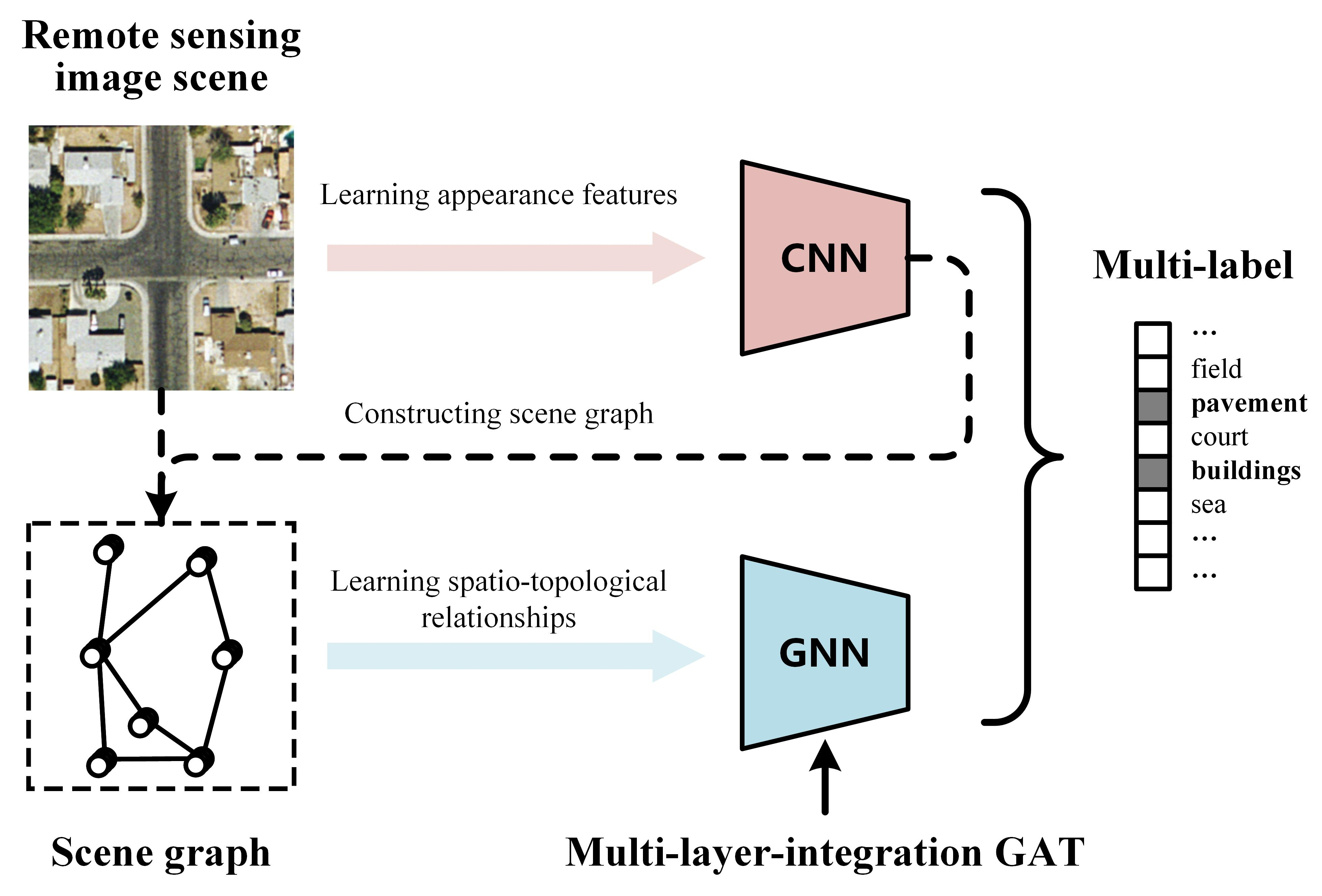
• We propose a novel MLRSSC-CNN-GNN framework that can simultaneously mine the appearances of visual elements in the scene and the spatio-topological relationships of visual elements. The experimental results on two public datasets demonstrate the effectiveness of our framework.
• We design a multi-layer-integration GAT model to mine the spatio-topological relationship of the RS image scene. Compared with the standard GAT, the recommended multi-layer-integration GAT benefits fusing multiple intermediate topological representations and can further improve the classification performance.

The remainder of this paper is organized as follows: Section 2 reviews the related works. Section 3 introduces the details of our proposed framework. Section 4 describes the setup of the experiments and reports the experimental results. Section 5 discusses the important factors of our framework. Section 6 presents the conclusions of this paper.

2. Related Work

In the following section, we specifically discuss the related works from two aspects: MLRSSC and GNN-based applications.

2.1. MLRSSC

In early research on MLRSSC, handcrafted features were often employed to describe image scenes [44,45]. However, handcrafted features have limited generalization ability and cannot achieve an optimal balance between discriminability and robustness. Recently, deep learning methods have achieved impressive results in MLRSSC [32,46]. For instance, the standard CNN method can complete feature extraction and classification end-to-end with a deep network framework. Moreover, Zeggada et al. designed a multi-label classification layer to address multi-label classification via customized threshold operation [33]. To exploit the co-occurrence dependency of multiple labels, Hua et al. combined the CNN and the RNN to sequentially predict labels [34]. However, due to the accumulation of misclassification information during the generation of label sequences, the use of the RNN may cause an error propagation problem [47]. Hua et al. also considered the label dependency and proposed a relation network for MLRSSC using the attention mechanism [48]. These methods are limited by only considering visual elements in the image scene but disregarding the spatio-topological relationships of visual elements. In addition, Kang et al. proposed a graph relation network to model the relationships between image scenes for MLRSSC [49]. However, it mainly focused on leveraging the relationship between image scenes, and still did not model the spatial relationship between visual elements in each image scene.

2.2. GNN-Based Applications

The GNN is a novel model with great potential that can extend the ability of deep learning to process non-Euclidean data. The GNN is extensively applied to the fields of social network [50], recommender system [51], knowledge graph [52], etc. In recent years, some GNNs, such as the GCN, have been employed to solve image understanding problems. Yang et al. constructed scene graphs for images and completed image captioning via the GCN [53]. Chaudhuri et al. used the Siamese GCN to assess the similarity of the scene graph for image retrieval [54]. Chen et al. proposed a GCN-based multi-label natural image classification model, where the GCN is employed to learn the label dependency [43]. However, the GCN is limited for exploring complex node relationships because it only uses a fixed or learnable polynomial of the adjacency matrix to aggregate node features. Compared with the GCN, the GAT is a more advanced model, which can learn the aggregation weights of nodes using the attention mechanism. The adaptability of the GAT can make it more effective to fuse information from graph topological structures and node features [55]. However, due to the difference between image data and graph-structured data, it is still a problem worth exploring to mine the spatio-topological relationship of images via GAT.

3. Method

To facilitate understanding, our proposed MLRSSC-CNN-GNN framework is visually shown in Figure 1. Generally, we propose a way to map an image into graph-structured data and transform the MLRSSC task into the graph classification task. Specifically, we consider the superpixel regions of the image scene as the nodes of the graph to construct the scene graph, where the node features are represented by the deep feature maps from the CNN. According to the proximity and similarity between superpixel regions, we define the adjacency of nodes, which can be easily employed by the GNN to optimize feature learning. With the scene graph as input, the multi-layer-integration GAT is designed to complete multi-label classification by fusing information from the node features and spatio-topological relationships of the graph.

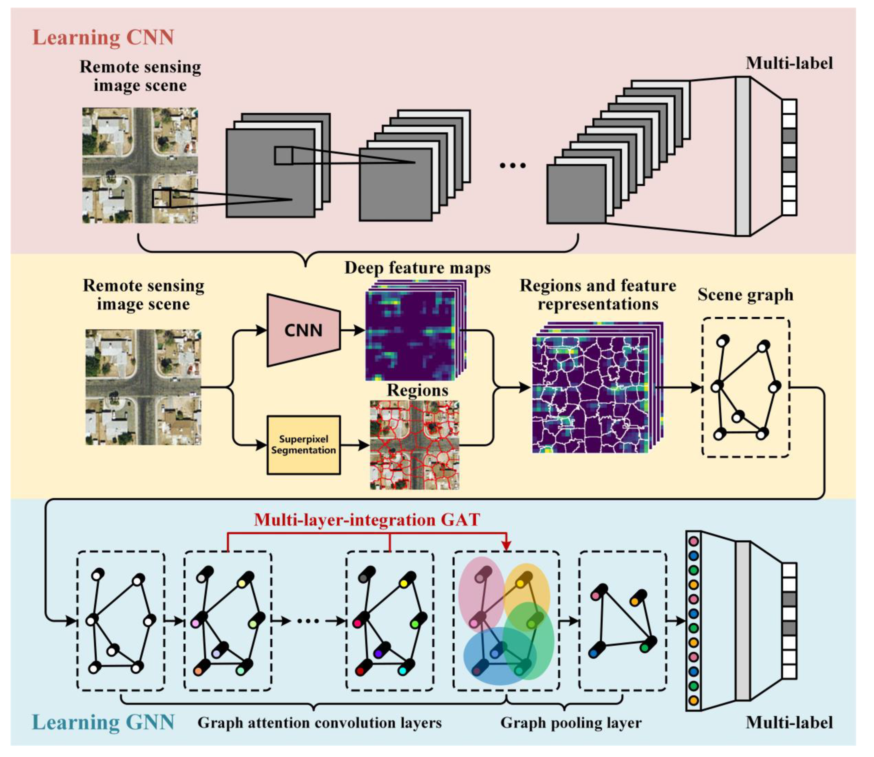
3.1. Using CNN to Generate Appearance Features

Generating visual representations of the image scene is crucial in our framework. In particular, we use the CNN as a feature extractor to obtain deep feature maps from intermediate convolutional layers as the representations of high-level appearance features. To improve the perception ability of the CNN and make it effective in the RS image, we retrain the CNN by transfer learning [56].

Considering $\Theta$ as the parameters of convolutional layers and $\Phi$ as the parameters of fully connected layers, the loss function during the training phase can be represented by Equation (1):

$$ℒ\left(\Theta ,\Phi \right)=-{\displaystyle \sum }_{c=1}^C\left(y^{\left(c\right)}\log \left(f_{CNN}{\left(I\right)}^{\left(c\right)}\right)+\left(1-y^{\left(c\right)}\right)\log \left(1-f_{CNN}{\left(I\right)}^{\left(c\right)}\right)\right),$$

(1)

where $f_{CNN}(\cdot )$ represents the nonlinear mapping process of the whole CNN network, $I$ indicates an RS image, $y^{\left(c\right)}$ indicates the ground truth binary label of class $c$, and $C$ is the number of categories. The process of feature extraction can be represented by Equation (2):

$$M=f_{FR}\left(I;\Theta \right),$$

(2)

where $f_{FR}(\cdot )$ represents the feature representation process of the trained CNN, and $M$ indicates the deep feature maps of image $I$.

Note that the CNN can also be trained from scratch using the RS image dataset. However, considering that the size of the experimental dataset is small, we choose to fine-tune the weights of the deep convolutional layers to quickly converge the model.

3.2. Constructing Scene Graph

We construct the scene graph for each image to map the image into graph-structured data. Graph-structure data are mainly composed of the node feature matrix $X\in {ℝ}^{N\times D}$ and the adjacency matrix $A\in {ℝ}^{N\times N}$, where $N$ is the number of nodes and $D$ is the dimension of features. In our framework, $X$ is constructed based on appearance features from the CNN, and $A$ is constructed according to the topological structure of the superpixel regions.

We use the simple linear iterative clustering (SLIC) superpixel algorithm [57] to segment the image and obtain $N$ nonoverlapping regions to represent the nodes of the graph. The SLIC is an unsupervised image segmentation method that uses k-means to locally cluster image pixels, which can generate a compact and nearly uniform superpixel. It is notable that the superpixel consists of homogeneous pixels, so it can be assumed that it is an approximate representation of local visual elements.

We apply the high-level appearance features as the initial node features to construct $X$. Specifically, we combine the deep feature maps $M$ and segmentation results by upsampling $M$ to the size of the original image. To catch the main visual features, we obtain the max value of the feature map slice according to each superpixel region boundary as the corresponding node feature. The node feature extraction will be repeated for each slice of $M$. Therefore, we can obtain multidimensional features from multiple channels of $M$ as the node features.

We construct $A$ considering the proximity and similarity between superpixel regions. We measure the spatial proximity of nodes by the adjacency of the superpixel regions and quantify the similarity of nodes by calculating the distance between superpixel regions in the color space, which satisfies human perception. In addition, we use the threshold of color distance to filter noisy links. When regions $i$ and $j$ have a common boundary, the adjacency value $A_{ij}$ is defined by Equation (3):

$$A_{ij}=\{\begin{array}{c}0, \mathrm{if} \Vert v_i-v_j\Vert >t\\ 1, \mathrm{if} \Vert v_i-v_j\Vert \le t\end{array},$$

(3)

where $v_i$ and $v_j$ represent the mean value of regions $i$ and $j$ in the HSV color space, and threshold $t$ is empirically set to 0.2 according to the common color aberration of different categories. Note that our $A$ is the symmetric binary matrix with the self-loop to define whether the nodes are connected. The specific adjacency weights will be adaptively learned in the GNN module to represent the relationships among nodes. The detailed process of constructing the scene graph is shown in Algorithm 1.

3.3. Learning GNN to Mine Spatio-Topological Relationship

Benefiting from the mechanism of node message passing, the GNN can integrate the spatio-topological structure into node feature learning. Thus, we treat the MLRSSC task as the graph classification task to mine the spatial relationships of the scene graph via the GNN. For graph classification, the GNN is composed of graph convolution layers, graph pooling layers and fully connected layers. Specifically, we adopt the GAT model [40] as the backbone of the graph convolution layer and design the multi-layer-integration GAT structure to better learn the complex spatial relationship and topological representations of the graph.

Algorithm 1 Algorithm to construct the scene graph of an RS image

Input: RS image $I$.

Output: Node feature matrix $X$ and adjacency matrix $A$.

1: for each $I$ do

2:  Extract deep feature maps $M$ from image $I$;

3:  Segment $I$ into $N$ superpixel regions $R$;

4:  for each $r\in R$ do

5:    Obtain the max values of $M$ according to the boundary of $r$ in $D$ channels, and update      the vector $X_r\in {ℝ}^D$ of the matrix $X$;

6:    Calculate the mean value $v_r$ of $r$ in the HSV color space;

7:    Obtain the adjacent regions list $R^{\prime }$ of $r$;

8:  end for

9:  for each $r\in R$ do

10:   $A_{rr}=1$;

11:   Calculate color distance $\Vert v_r-v_{r^{\prime }}\Vert$ between $r$ and $r^{\prime }\in R^{\prime }$;

12:   if $\Vert v_r-v_{r^{\prime }}\Vert \le t$ do

13:    $A_{r{r}^{\prime }}=1$;

14:   end if

15:  end for

16: end for

3.3.1. Graph Attention Convolution Layer

We construct the graph convolution layer following the GAT model to constantly update the node features and adjacency weights. With the attention mechanism, the adjacency weights are adaptively learned according to the node features, which can represent the complex relationships among nodes. Considering $X_i\in {ℝ}^D$ as the features of node $i$, the attention weight $e_{ij}$ between node $i$ and node $j$ is calculated with a learnable linear transformation, which can be represented by Equation (4):

$$e_{ij}=H^T[W{X}_i\Vert W{X}_j],$$

(4)

where $\Vert$ is the concatenation operation, $W\in {ℝ}^{D^{\prime }\times D}$ and $H\in {ℝ}^{2D^{’}}$ are the learnable parameters, and $D^{\prime }$ indicates the dimension of the output features. The topological structure is injected into the mechanism by a mask operation. Specifically, only $e_{ij}$ for nodes $j\in {\mathsf{\eta }}_i$ are employed in the network, where ${\mathsf{\eta }}_i$ is the neighborhood of node $i$, which is generated according to $A$. Subsequently, $e$ is nonlinearly activated via the LeakyReLU function and normalized by Equation (5):

$${\alpha }_{ij}=\frac{\exp \left(\mathrm{LeakyReLU}\left(e_{ij}\right)\right)}{{{\displaystyle \sum }}_{z\in {\mathsf{\eta }}_i}\exp \left(\mathrm{LeakyReLU}\left(e_{iz}\right)\right)}.$$

(5)

We can fuse information from the graph topological structures and node features by matrix multiplication between $\alpha$ and $X$. In addition, we adopt multi-head attention to stabilize the learning process. Considering $X_{in}\in {ℝ}^{N\times D}$ as the input node features, the output node features $X_{GAT}\in {ℝ}^{N\times K{D}^{’}}$ of a graph attention convolution layer can be computed by Equation (6):

$$X_{GAT}={\Vert }_{k=1}^K\mathrm{ReLU}\left({\alpha }^{\left(k\right)}{X}_{in}{W}^{\left(k\right)}\right),$$

(6)

where $\Vert$ represents the concatenation operation, ${\alpha }^{\left(k\right)}$ is the normalized attention matrix of the k-th attention mechanism, and $W^{\left(k\right)}$ is the corresponding weight matrix. Equation (6), represents the concatenation of the output node features from $K$ independent attention mechanisms.

To synthesize the advantage of each graph attention convolution layer and obtain comprehensive representation of the graph, we design the multi-layer-integration GAT structure that is shown in Figure 1. After multiple graph attention convolution layers, the hierarchical features of the same node are summarized as the new node features $X_{mGAT}$, which can be computed by Equation (7):

$$X_{mGAT}={\displaystyle \sum }_{l=1}^L{X}_{GAT}{}^{\left(l\right)},$$

(7)

where $X_{GAT}{}^{\left(l\right)}$ represents the output node features of the l-th graph attention convolution layer, and $L$ is the total number of graph attention convolution layers.

3.3.2. Graph Pooling Layer

For graph classification, we use a graph pooling layer to convert a graph of any size to a fixed-size output. Specifically, we adopt differentiable pooling proposed in [58] to construct the graph pool layer. The idea of differentiable pooling is to transform the original graph into a coarsened graph through the way of embedded. Considering $X_{in}\in {ℝ}^{N\times D}$ as the input node features and $N^{\prime }$ as the new number of nodes, the embedded matrix $S\in {ℝ}^{N\times N^{\prime }}$ can be learned by Equation (8):

$$S=\mathrm{softmax}\left(X_{in}{W}_{emb}+b_{emb}\right),$$

(8)

where $W_{emb}\in {ℝ}^{D\times N^{\prime }}$ represents the learnable weight and $b_{emb}$ is the bias. The softmax function is applied in a row-wise function. The node feature matrix output $X_{GP}\in {ℝ}^{N^{\prime }\times D}$ of a graph pooling layer can be calculated by Equation (9):

$$X_{GP}=S^T{X}_{in}.$$

(9)

Because the graph pooling operation is learnable, the output graph is an optimized result that represents the reduced-dimension input graph.

3.3.3. Classification Layer

After graph pooling, we flatten the node features matrix and obtain a finite dimensional vector to represent the global representation of the graph. Taking $X_{in}$ as the input node features, the flatten operation can be represented by Equation (10):

$$x=\mathrm{flatten}\left(X_{in}\right),$$

(10)

where $x$ is a feature vector. At the end of the network, we add fully connected layers followed by the sigmoid activation function as the classifier to complete the graph classification. The classification probability output $\widehat{y}$ of the last fully connected layer can be computed by Equation (11):

$$\widehat{y}=\sigma \left(x{W}_{fc}+b_{fc}\right),$$

(11)

where $\sigma (\cdot )$ is the sigmoid function, $W_{fc}$ represents the learnable weight and $b_{fc}$ is the bias. Furthermore, we apply the binary cross-entropy as the loss function, which can be defined by Equation (12):

$$ℒ\left(\Lambda \right)=-{\displaystyle \sum }_{c=1}^C\left(y^{\left(c\right)}\log \left({\widehat{y}}^{\left(c\right)}\right)+\left(1-y^{\left(c\right)}\right)\log \left(1-{\widehat{y}}^{\left(c\right)}\right)\right),$$

(12)

where $\Lambda$ represents the parameters of the whole GNN network and $y^{\left(c\right)}$ indicates the ground truth binary label of class $c$. Via back-propagation, $\Lambda$ can be optimized based on the gradient of the loss. Thus, we can use GNN to complete the multi-label classification in an end-to-end manner. The training process of the whole MLRSSC-CNN-GNN framework is shown in Algorithm 2.

4. Experiments

In this section, the data description is presented at first. Afterwards, the evaluation metrics and details of the experimental setting are shown. The experimental results and analysis are given at the end.

Algorithm 2 Training process of the proposed MLRSSC-CNN-GNN framework

Input: RS images $I$ and ground truth multi-labels $y$ in training set.

Output: Model parameters $\Theta$ and $\Lambda$.    Step 1: Learning CNN

1: Take $I$ and $y$ as input, and train CNN to optimize $\Theta$ according to Equation (1);

2: Extract deep feature maps $M$ of $I$ according to Equation (2);    Step 2: Constructing scene graph

3: Construct node feature matrix $X$ and adjacency matrix $A$ of $I$ according to Algorithm 1;    Step 3: Learning GNN

4: for $iter=1,2,\dots$ do

5:    Initialize parameters $\Lambda$ of the network in the first iteration;

6:    Update $X$ using $L$ graph attention convolution layers according to Equation (4)–(6);

7:    Fuse $X_{GAT}$ from $L$ graph attention convolution layers according to Equation (7);

8:    Cover $X_{mGAT}$ to a fixed-size output via the graph pooling layer according to Equation (8-9);

9:    Flatten $X_{GP}$ and generate the classification probability after the classification layer according to Equation (10-11);

10:    Calculate the loss based on the output $\widehat{y}$ of the network and $y$ according to Equation (12);

11:    Update $\Lambda$ by back-propagation;

10: end for

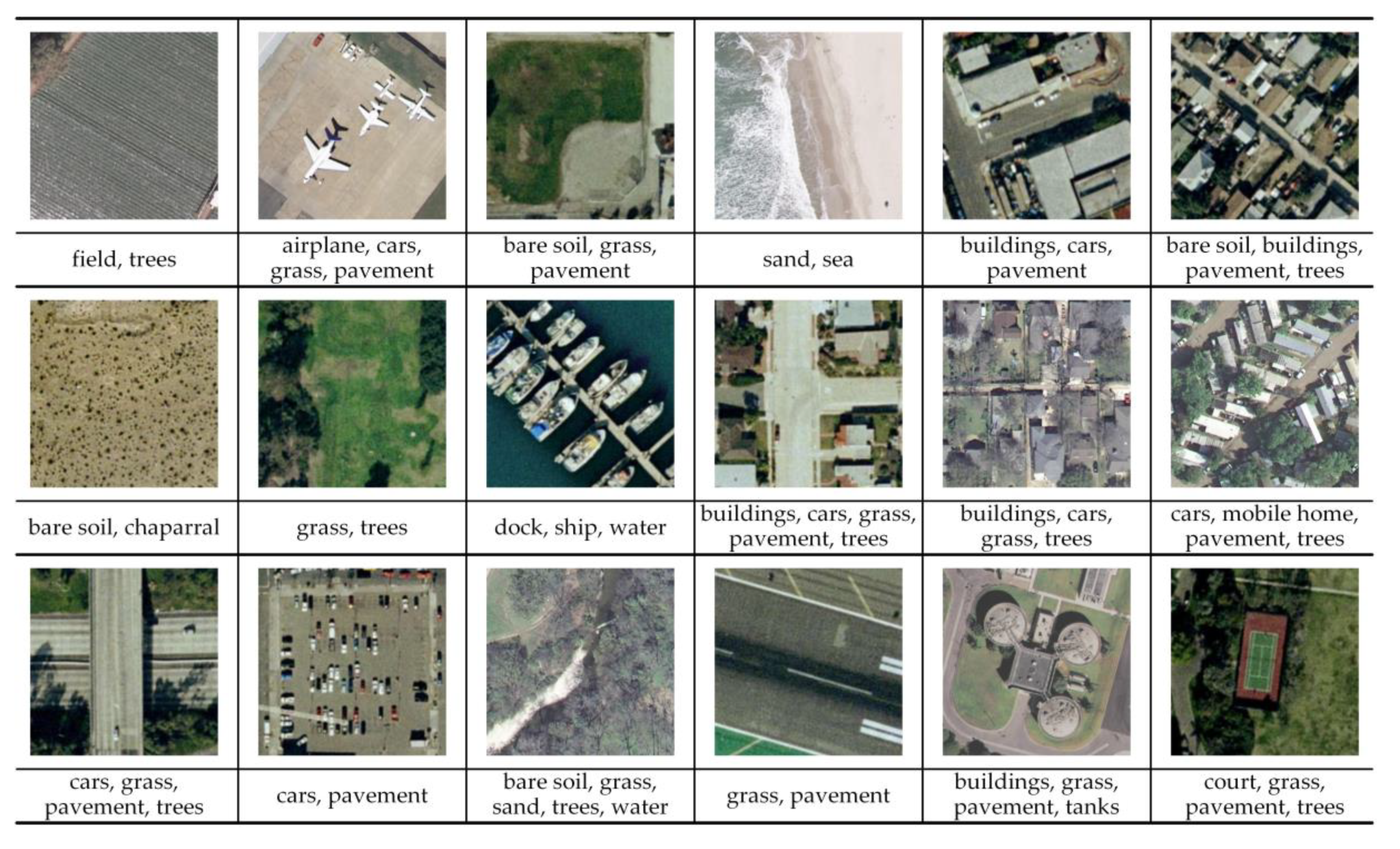
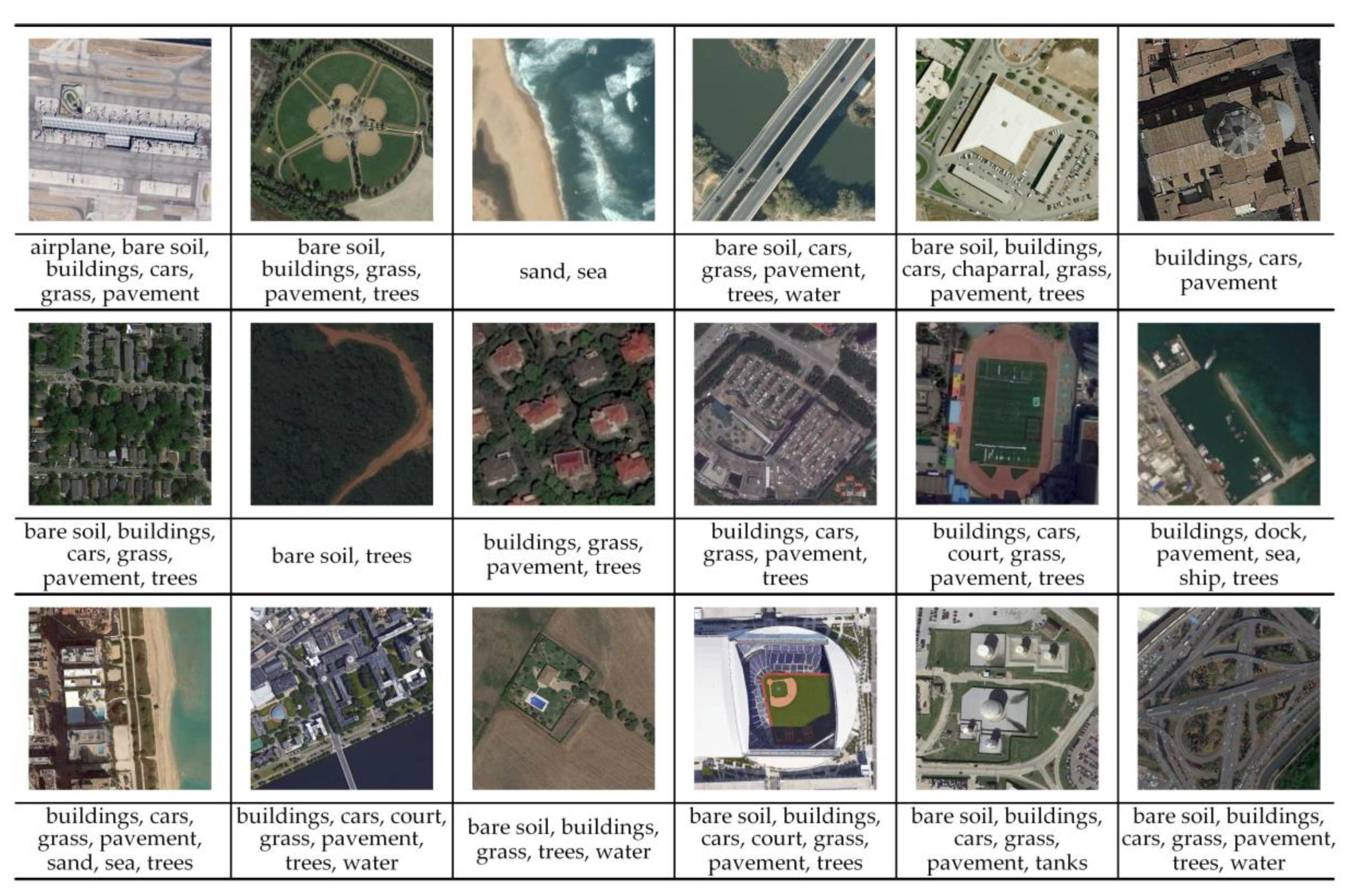
4.1. Dataset Description

We perform experiments on the UCM multi-label dataset and AID multi-label dataset, which are described here. The UCM multi-label dataset contains 2100 RS images with 0.3 m/pixel spatial resolution, and the image size is 256 × 256 pixels. For MLRSSC, the dataset is divided into the following 17 categories based on the DLRSD dataset [59]: airplane, bare soil, buildings, cars, chaparral, court, dock, field, grass, mobile home, pavement, sand, sea, ship, tanks, trees, and water. Some example images and their labels are shown in Figure 2.

The AID multi-label dataset [48] contains 3000 RS images from the AID dataset [60]. For MLRSSC, the dataset is assigned 17 categories, which are the same as those in the UCM multi-label dataset. The spatial resolutions of the images vary from 0.5 m/pixel to 0.8 m/pixel, and the size of each image is 600 × 600 pixels. Some example images and their labels are shown in Figure 3.

4.2. Evaluation Metrics

We calculate Precision, Recall, F1-Score and F2-Score to evaluate the multi-label classification performance [61]. The evaluation indicators are computed based on the number of true positives (TP), false positives (FP), true negatives (TN) and false negatives (FN) in an example (i.e., an image with multiple labels). The evaluation indicators can be calculated using Equations (13) and (14):

$$\mathrm{Precision}=\frac{\mathrm{TP}}{\mathrm{TP}+\mathrm{FP}},\mathrm{Recall}=\frac{\mathrm{TP}}{\mathrm{TP}+\mathrm{FN}},$$

(13)

$${\mathrm{F}\mathsf{\beta }}_{\mathrm{Score}}=\left(1+{\mathsf{\beta }}^2\right)\frac{\mathrm{Precision}·\mathrm{Recall}}{{\mathsf{\beta }}^2·\mathrm{Precision}+\mathrm{Recall}},\mathsf{\beta }=1,2.$$

(14)

Note that all the evaluation indicators are example-based indices that are formed by averaging the scores of each individual sample [62]. Generally, F1-Score and F2-Score are relatively more important for performance evaluation.

4.3. Experimental Settings

In our experiments, we adopt VGG16 [63] as the CNN backbone. The network is initialized with the weights trained on ImageNet [64], and we fine-tune it with the experimental datasets. In addition, we use fusion features by combining feature maps from the “block4_conv3” and “block5_conv3” layers in VGG16 as the node features of the scene graph. Thus, the total dimension of the initial node features is 1024.

Our recommended GNN architecture contains two graph attention convolution layers with the output dimensions of 512 and multi-head attention with $K=3$. The multi-layer-integration GAT structure is applied to construct the graph attention convolution layers. Subsequently, we set up one graph pooling layer that fixes the size of the graph to 32 nodes and two fully connected layers with the output dimensions of 256 and 17 (number of categories). Moreover, the dropout layer is set in the middle of each layer, and batch normalization is employed for all layers but the last layer. The network is trained with the Adagrad optimizer [65], and the learning rate is initially set to 0.01, which decays during the training process.

To pursue a fair comparison, based on the partition way in [48], the UCM and AID multi-label datasets are split into 72% for training, 8% for validation and 20% for testing. Note that instead of randomly division, this partition way is pre-set, where the training and testing samples have obvious style differences. Therefore, it will be more challenging for the classification methods. In the training phase, we only use the training images and their ground truth labels to train the CNN and the GNN. Specifically, we learn the CNN to extract deep feature maps of the images and then construct a scene graph for each image, which is the input of the GNN. In the testing phase, the testing images are fed into the trained CNN and GNN models to predict multi-labels.

4.4. Comparison with the State-of-the-Art Methods

We compare our proposed methods with several recent methods, including the standard CNN [63], CNN-RBFNN [33], CA-CNN-BiLSTM [34] and AL-RN-CNN [48]. For a fair comparison, all compared methods adopt the same VGG16 structure as the CNN backbone. We implement the standard CNN method as the baseline of MLRSSC and report the mean and standard deviation [66] of the evaluation results. Because the other methods also adopt the same dataset partition, we take the reported evaluation results from their corresponding publications as the comparison reference in this paper. It is noted that the existing methods don’t report the standard deviation of evaluation results. As these methods don’t release their source codes, it is hard to recover the standard deviation of the existing methods. Fortunately, we find the variance of repeated experiments is very slight, which helps to fully show the superiority of our proposed method. For the proposed methods, we report the results based on the MLRSSC-CNN-GNN via the standard GAT and the MLRSSC-CNN-GNN via the multi-layer-integration GAT, respectively.

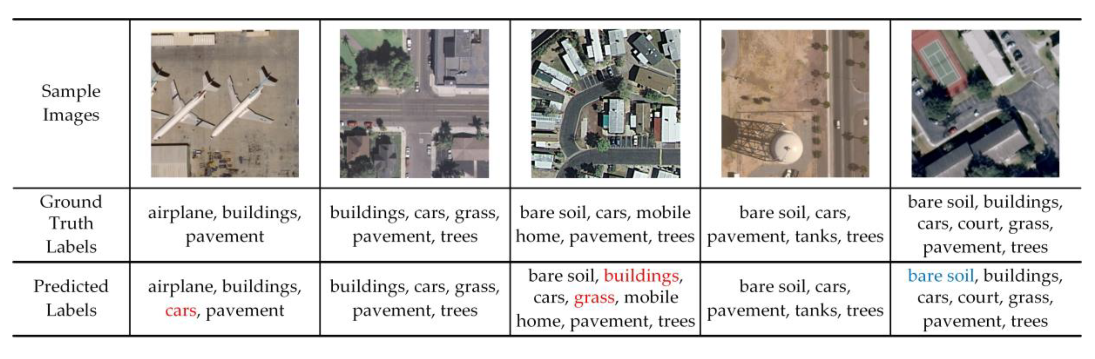
4.4.1. Results on the UCM Multi-Label Dataset

The quantitative results on the UCM multi-label dataset are shown in

Table 1. Performances of different methods on the UCM multi-label dataset (%).

Methods	Precision	Recall	F1-Score	F2-Score
CNN [63]	80.09 ± 0.25	81.78 ± 0.41	78.99 ± 0.10	80.18 ± 0.09
CNN-RBFNN [33]	78.18	83.91	78.80	81.14
CA-CNN-BiLSTM [34]	79.33	83.99	79.78	81.69
AL-RN-CNN [48]	87.62	86.41	85.70	85.81
Our MLRSSC-CNN-GNN via standard GAT	86.41 ± 0.22	88.17 ± 0.09	86.09 ± 0.07	87.03 ± 0.02
Our MLRSSC-CNN-GNN via multi-layer-integration GAT	87.11 ± 0.09	88.41 ± 0.10	86.39 ± 0.04	87.27 ± 0.07

. We can observe that our proposed MLRSSC-CNN-GNN via the multi-layer-integration GAT achieves the highest scores for Recall, F1-Score and F2-Score. In general, the proposed method achieves the best performance. The lower bound of our method can also be better than the performances of the existing methods. We can also observe that our methods with the GNN show significant improvement compared with the method that only uses the CNN. Compared with the standard CNN, the proposed method gains an improvement of 7.4% for F1-Score and an improvement of 7.09% for F2-Score, which demonstrates that learning the spatial relationship of visual elements via the GNN has an important role in advancing the classification performances. Moreover, the MLRSSC-CNN-GNN via the multi-layer-integration GAT performs better than the MLRSSC-CNN-GNN via the standard GAT, which shows the effectiveness of the proposed multi-layer-integration GAT.

Some samples of the predicted results on the UCM multi-label dataset are exhibited in Figure 4. It can be seen that the proposed method can successfully capture the main categories of the scene. However, our method is still insufficient in the details, such as the prediction of cars, grass, and bare soil, which may be inconsistent with the ground truths.

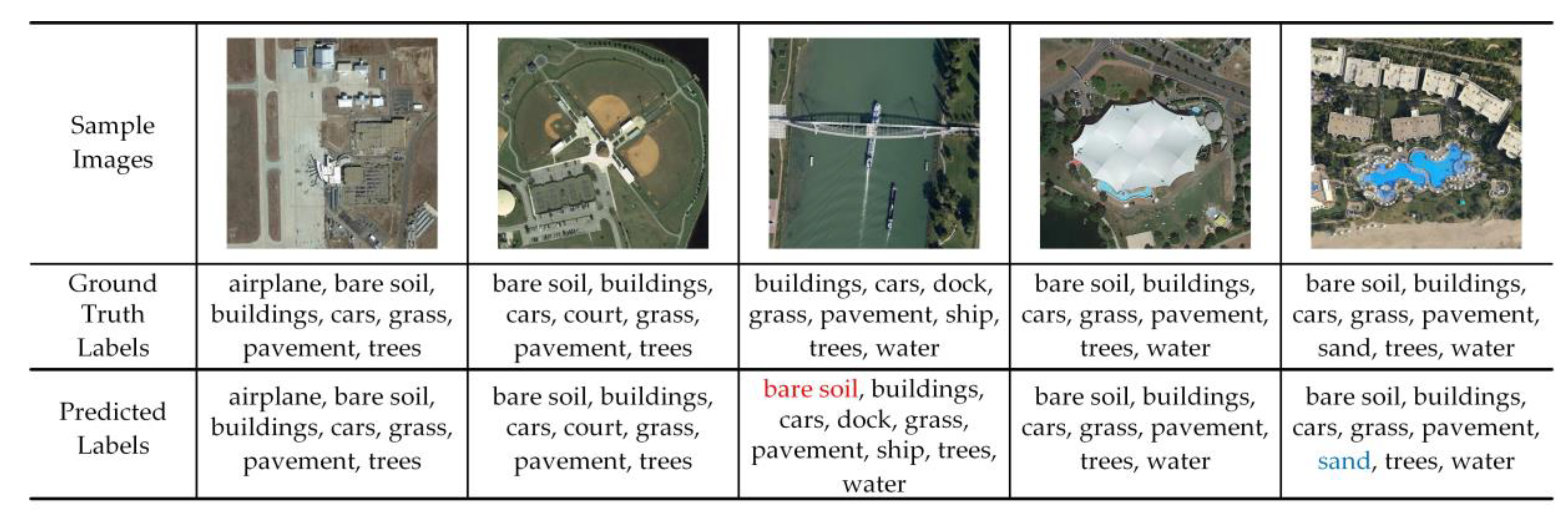
4.4.2. Results on the AID Multi-Label Dataset

Table 2. Performances of different methods on the AID multi-label dataset (%).

Methods	Precision	Recall	F1-Score	F2-Score
CNN [63]	87.62 ± 0.14	86.13 ± 0.15	85.31 ± 0.09	85.36 ± 0.07
CNN-RBFNN [33]	84.56	87.85	84.58	85.99
CA-CNN-BiLSTM [34]	88.68	87.83	86.68	86.88
AL-RN-CNN [48]	89.96	89.27	88.09	88.31
Our MLRSSC-CNN-GNN via standard GAT	89.78 ± 0.24	89.52 ± 0.10	88.32 ± 0.05	88.66 ± 0.05
Our MLRSSC-CNN-GNN via multi-layer-integration GAT	89.83 ± 0.27	90.20 ± 0.22	88.64 ± 0.06	89.18 ± 0.13

shows the experimental results on the AID multi-label dataset. We can also observe that our proposed MLRSSC-CNN-GNN via the multi-layer-integration GAT achieves the best performance with the highest scores of Recall, F1-Score and F2-Score. Compared to the standard CNN, the proposed method increases F1-Score and F2-Score by 3.33% and 3.82%, respectively. Compared to AL-RN-CNN, the proposed method gains an improvement of 0.55% for F1-Score and an improvement of 0.87% for F2-Score. Compared to the MLRSSC-CNN-GNN via the GAT, the proposed method gains an improvement of 0.32% for F1-Score and an improvement of 0.52% for F2-Score.

Some samples of the predicted results on the AID multi-label dataset are exhibited in Figure 5. Consistent with the results on the UCM multi-label dataset, our method can successfully capture the main categories of the scene. The superior performances on both UCM and AID multi-label datasets can show the robustness and effectiveness of our method.

5. Discussion

In this section, we analyze the influence of some important factors in the proposed framework, including the number of superpixel regions in the scene graph, the value K of multi-head attention in the GNN, and the depth of the GNN.

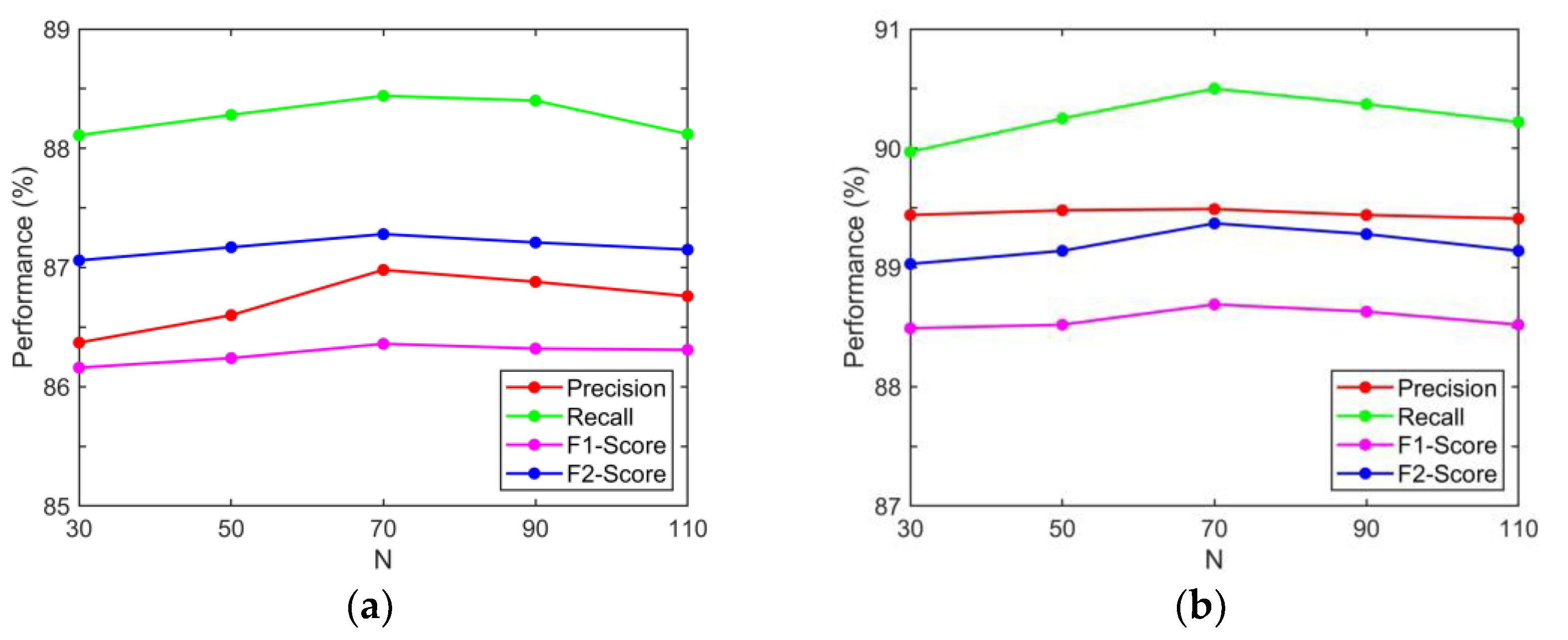
5.1. Effect on the Number of Superpixel Regions

When constructing the scene graph, the number of superpixel regions $N$ is a vital parameter, which determines the scale and granularity of the initial graph. Therefore, it is necessary to set an appropriate $N$. Considering the tradeoff between efficiency and performance, we set the step size of the $N$ to 20, and study the effects of $N$ by setting it from 30 to 110. The results on the UCM and AID multi-label datasets are shown in Figure 6. It can be seen that when the $N$ is set between 50 to 90, our model can achieve better performance.

5.2. Sensitivity Analysis of the Multi-Head Attention

In the graph attention convolution layer of the GNN, we adopt multi-head attention to stabilize the learning process. However, a larger value of $K$ in multi-head attention will increase the parameters and calculation of the model. Thus, we study the effects of $K$ by setting it to a value from 1 to 5. The experimental results on the UCM and AID multi-label datasets are shown in Figure 7. Obviously, the use of multi-head attention can improve the classification performance because it can learn more abundant feature representations. It can be seen that when the value of $K$ reaches 3, the performance of the model begins to saturate. However, when the value of $K$ continues to increase, the model may face an overfitting problem.

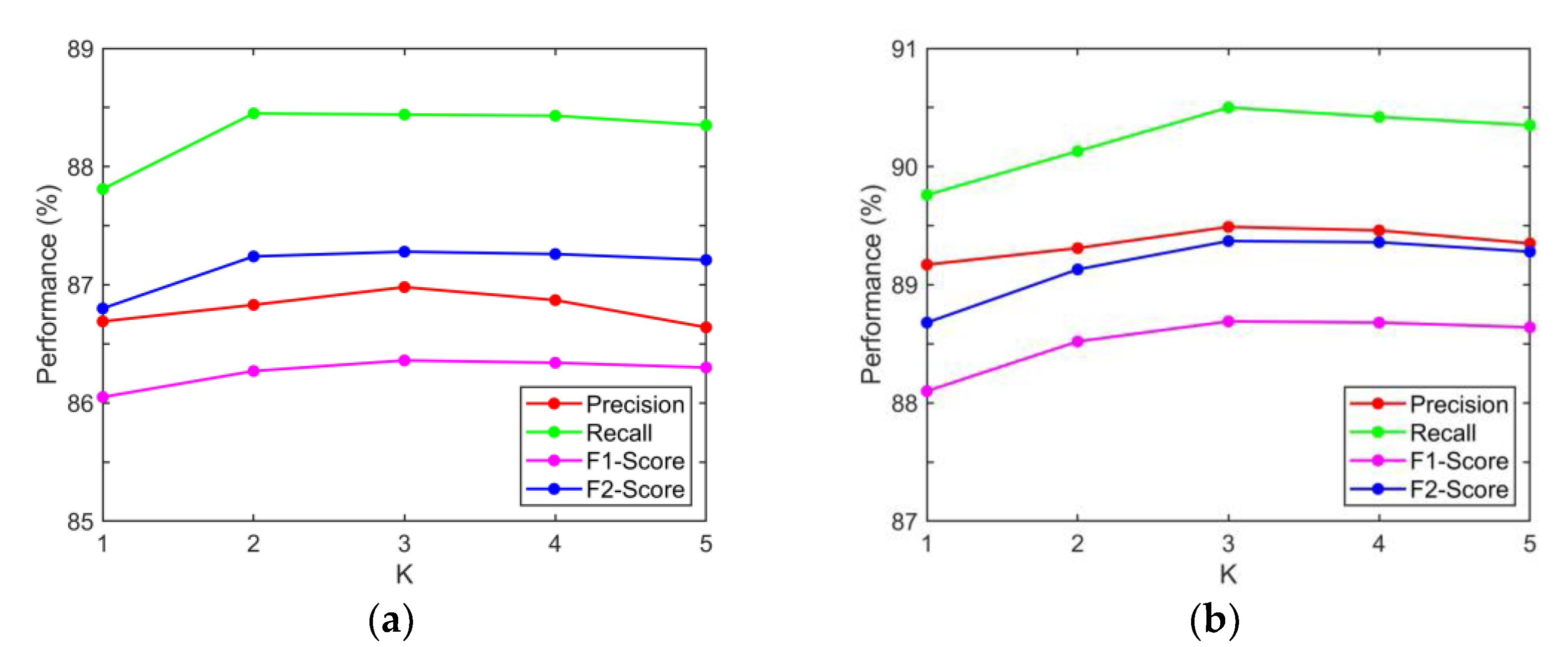
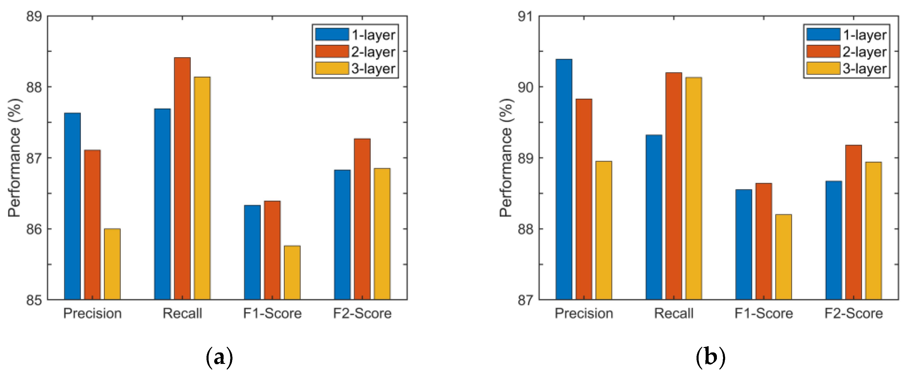
5.3. Discussion on the Depth of GNN

The graph attention convolution layer in the GNN is the key part to learning the classification features of the graph. To explore the performance of the GNN in our framework, we build the GNN with a different number of graph attention convolution layers. Figure 8 shows the performance of our MLRSSC-CNN-GNN with one, two, and three graph attention convolution layers. The output dimensions of these layers are 512, and the remaining structures in GNN are the same. It can be seen that the MLRSSC-CNN-GNN with two graph attention convolution layers achieves the best performance with the highest F1-Score and F2-Score. However, when the number of graph attention convolution layers reaches three, both the F1-Score and F2-Score begin to drop. The possible reason for the performance drop of the deep GNN may be that the node features are oversmoothed when a larger number of graph attention convolution layers are utilized.

6. Conclusions

MLRSSC remains a challenging task because it is difficult to learn the discriminative semantic representations to distinguish multiple categories. Although many deep learning-based methods have been proposed to address MLRSSC and achieved a certain degree of success, the existing methods are limited by only perceiving visual elements in the scene but disregarding the spatial relationships of visual elements. With this consideration, this paper proposes a novel MLRSSC-CNN-GNN framework to address MLRSSC. Different from the existing methods, the proposed method can comprehensively utilize the visual and spatial information in the scene by combining the CNN and the GNN. Specifically, we encode the visual content and spatial structure of the RS image scene by constructing scene graph. The CNN and the GNN is used to mine the appearance features and spatio-topological relationships, respectively. In addition, we design the multi-layer-integration GAT model to further mine the topological representations of scene graph for classification. The proposed framework is verified on two public MLRSSC datasets. As the experimental results shown, the proposed method can improve both the F1-Score and F2-Score by more than 3%, which demonstrates the importance of learning spatio-topological relationships via the GNN. Moreover, the proposed method can obtain superior performances compared with the state-of-the-art methods. As a general framework, the proposed MLRSSC-CNN-GNN framework is highly flexible, it can be easily and dynamically enhanced by replacing the corresponding modules with advanced algorithms. In future work, we will consider the adoption of more advanced CNN and GNN models to explore the potential of our framework. However, our proposed method has not explicitly modeled label dependency, which is also important in MLRSSC. In the future, we will focus on integrating this consideration into our method to further improve the performance.

References

1. Cheng, G.; Han, J.; Guo, L.; Liu, Z.; Bu, S.; Ren, J. Effective and efficient midlevel visual elements-oriented land-use classification using VHR remote sensing images. IEEE Trans. Geosci. Remote Sens. 2015, 53, 4238–4249. [Google Scholar] [CrossRef] [Green Version]
2. Li, Y.; Tao, C.; Tan, Y.; Shang, K.; Tian, J. Unsupervised multilayer feature learning for satellite image scene classification. IEEE Geosci. Remote Sens. Lett. 2016, 13, 157–161. [Google Scholar] [CrossRef]
3. Li, Y.; Zhang, Y.; Zhu, Z. Error-tolerant deep learning for remote sensing image scene classification. IEEE Trans. Cybern 2020, in press. [Google Scholar] [CrossRef] [PubMed]
4. Han, J.; Zhou, P.; Zhang, D.; Cheng, G.; Guo, L.; Liu, Z.; Bu, S.; Wu, J. Efficient, simultaneous detection of multi-class geospatial targets based on visual saliency modeling and discriminative learning of sparse coding. ISPRS J. Photogramm. Remote Sens. 2014, 89, 37–48. [Google Scholar] [CrossRef]
5. Li, Y.; Chen, W.; Zhang, Y.; Tao, C.; Xiao, R.; Tan, Y. Accurate cloud detection in high-resolution remote sensing imagery by weakly supervised deep learning. Remote Sens. Environ. 2020, 250, 112045. [Google Scholar] [CrossRef]
6. Tao, C.; Mi, L.; Li, Y.; Qi, J.; Xiao, Y.; Zhang, J. Scene context-driven vehicle detection in high-resolution aerial images. IEEE Trans. Geosci. Remote Sens. 2019, 57, 7339–7351. [Google Scholar] [CrossRef]
7. Li, Y.; Zhang, Y.; Huang, X.; Yuille, A.L. Deep networks under scene-level supervision for multi-class geospatial object detection from remote sensing images. ISPRS J. Photogramm. Remote Sens. 2018, 146, 182–196. [Google Scholar] [CrossRef]
8. Li, Y.; Zhang, Y.; Huang, X.; Ma, J. Learning source-invariant deep hashing convolutional neural networks for cross-source remote sensing image retrieval. IEEE Trans. Geosci. Remote Sens. 2018, 56, 6521–6536. [Google Scholar] [CrossRef]
9. Li, Y.; Zhang, Y.; Huang, X.; Zhu, H.; Ma, J. Large-scale remote sensing image retrieval by deep hashing neural networks. IEEE Trans. Geosci. Remote Sens. 2018, 56, 950–965. [Google Scholar] [CrossRef]
10. Li, Y.; Ma, J.; Zhang, Y. Image retrieval from remote sensing big data: A survey. Inf. Fusion. 2021, 67, 94–115. [Google Scholar] [CrossRef]
11. Jian, L.; Gao, F.; Ren, P.; Song, Y.; Luo, S. A noise-resilient online learning algorithm for scene classification. Remote Sens. 2018, 10, 1836. [Google Scholar] [CrossRef] [Green Version]
12. Zhang, W.; Tang, P.; Zhao, L. Remote sensing image scene classification using CNN-CapsNet. Remote Sens. 2019, 11, 494. [Google Scholar] [CrossRef] [Green Version]
13. Sun, H.; Li, S.; Zheng, X.; Lu, X. Remote sensing scene classification by gated bidirectional network. IEEE Trans. Geosci. Remote Sens. 2020, 58, 82–96. [Google Scholar] [CrossRef]
14. Cheng, G.; Xie, X.; Han, J.; Guo, L.; Xia, G.-S. Remote Sensing Image Scene Classification Meets Deep Learning: Challenges, Methods, Benchmarks, and Opportunities. IEEE J. Sel. Top. Appl. Earth Obs. Remote Sens. 2020, 13, 3735–3756. [Google Scholar] [CrossRef]
15. Chen, K.; Jian, P.; Zhou, Z.; Guo, J.; Zhang, D. Semantic Annotation of High-Resolution Remote Sensing Images via Gaussian Process Multi-Instance Multilabel Learning. IEEE Geosci. Remote Sens. Lett. 2013, 10, 1285–1289. [Google Scholar] [CrossRef]
16. Han, X.-H.; Chen, Y. Generalized aggregation of sparse coded multi-spectra for satellite scene classification. ISPRS Int. J. Geo-Inf. 2017, 6, 175. [Google Scholar] [CrossRef] [Green Version]
17. Nogueira, K.; Penatti, O.A.B.; dos Santos, J.A. Towards better exploiting convolutional neural networks for remote sensing scene classification. Pattern Recognit. 2017, 61, 539–556. [Google Scholar] [CrossRef] [Green Version]
18. Chaudhuri, B.; Demir, B.; Chaudhuri, S.; Bruzzone, L. Multilabel Remote Sensing Image Retrieval Using a Semisupervised Graph-Theoretic Method. IEEE Trans. Geosci. Remote Sens. 2018, 56, 1144–1158. [Google Scholar] [CrossRef]
19. Tan, Q.; Liu, Y.; Chen, X.; Yu, G. Multi-label classification based on low rank representation for image annotation. Remote Sens. 2017, 9, 109. [Google Scholar] [CrossRef] [Green Version]
20. Everingham, M.; Van Gool, L.; Williams, C.K.I.; Winn, J.; Zisserman, A. The pascal visual object classes (VOC) challenge. Int. J. Comput. Vis. 2010, 88, 303–338. [Google Scholar] [CrossRef] [Green Version]
21. Lin, T.-Y.; Maire, M.; Belongie, S.; Hays, J.; Perona, P.; Ramanan, D.; Dollár, P.; Zitnick, C.L. Microsoft COCO: Common objects in context. In Proceedings of the 2014 European Conference on Computer Vision (ECCV), Zurich, Switzerland, 6–12 September 2014; pp. 740–755. [Google Scholar]
22. Krishna, R.; Zhu, Y.; Groth, O.; Johnson, J.; Hata, K.; Kravitz, J.; Chen, S.; Kalantidis, Y.; Li, L.-J.; Shamma, D.A.; et al. Visual genome: Connecting language and vision using crowdsourced dense image annotations. Int. J. Comput. Vis. 2017, 123, 32–73. [Google Scholar] [CrossRef] [Green Version]
23. He, K.; Zhang, X.; Ren, S.; Sun, J. Deep residual learning for image recognition. In Proceedings of the 2016 IEEE Conference on Computer Vision and Pattern Recognition (CVPR), Las Vegas, NV, USA, 27–30 June 2016; pp. 770–778. [Google Scholar]
24. Xie, S.; Girshick, R.; Dollar, P.; Tu, Z.; He, K. Aggregated residual transformations for deep neural networks. In Proceedings of the 2017 IEEE Conference on Computer Vision and Pattern Recognition (CVPR), Honolulu, HI, USA, 21–26 July 2017; pp. 5987–5995. [Google Scholar]
25. Zhang, X.; Zhou, X.; Lin, M.; Sun, J. ShuffleNet: An extremely efficient convolutional neural network for mobile devices. In Proceedings of the 2018 IEEE/CVF Conference on Computer Vision and Pattern Recognition, Salt Lake City, UT, USA, 18–23 June 2018; pp. 6848–6856. [Google Scholar]
26. Yang, H.; Zhou, J.T.; Zhang, Y.; Gao, B.-B.; Wu, J.; Cai, J. Exploit bounding box annotations for multi-label object recognition. In Proceedings of the 2016 IEEE Conference on Computer Vision and Pattern Recognition (CVPR), Las Vegas, NV, USA, 27–30 June 2016; pp. 280–288. [Google Scholar]
27. Badrinarayanan, V.; Kendall, A.; Cipolla, R. SegNet: A deep convolutional encoder-decoder architecture for image segmentation. IEEE Trans. Pattern Anal. Mach. Intell. 2017, 39, 2481–2495. [Google Scholar] [CrossRef] [PubMed]
28. Wang, J.; Yang, Y.; Mao, J.; Huang, Z.; Huang, C.; Xu, W. CNN-RNN: A unified framework for multi-label image classification. In Proceedings of the 2016 IEEE Conference on Computer Vision and Pattern Recognition (CVPR), Las Vegas, NV, USA, 27–30 June 2016; pp. 2285–2294. [Google Scholar]
29. Zhang, J.; Wu, Q.; Shen, C.; Zhang, J.; Lu, J. Multilabel image classification with regional latent semantic dependencies. IEEE Trans. Multimedia 2018, 20, 2801–2813. [Google Scholar] [CrossRef] [Green Version]
30. Zhu, X.X.; Tuia, D.; Mou, L.; Xia, G.-S.; Zhang, L.; Xu, F.; Fraundorfer, F. Deep learning in remote sensing: A comprehensive review and list of resources. IEEE Geosci. Remote Sens. Mag. 2017, 5, 8–36. [Google Scholar] [CrossRef] [Green Version]
31. Lobry, S.; Marcos, D.; Murray, J.; Tuia, D. RSVQA: Visual question answering for remote sensing data. IEEE Trans. Geosci. Remote Sens. 2020, 58, 8555–8566. [Google Scholar] [CrossRef]
32. Stivaktakis, R.; Tsagkatakis, G.; Tsakalides, P. Deep learning for multilabel land cover scene categorization using data augmentation. IEEE Geosci. Remote Sens. Lett. 2019, 16, 1031–1035. [Google Scholar] [CrossRef]
33. Zeggada, A.; Melgani, F.; Bazi, Y. A deep learning approach to UAV image multilabeling. IEEE Geosci. Remote Sens. Lett. 2017, 14, 694–698. [Google Scholar] [CrossRef]
34. Hua, Y.; Mou, L.; Zhu, X.X. Recurrently exploring class-wise attention in a hybrid convolutional and bidirectional LSTM network for multi-label aerial image classification. ISPRS J. Photogramm. Remote Sens. 2019, 149, 188–199. [Google Scholar] [CrossRef]
35. Lee, J.; Lee, I.; Kang, J. Self-attention graph pooling. In Proceedings of the 2019 International Conference on Machine Learning (ICML), Long Beach, CA, USA, 9–15 June 2019; pp. 6661–6670. [Google Scholar]
36. Such, F.P.; Sah, S.; Dominguez, M.A.; Pillai, S.; Zhang, C.; Michael, A.; Cahill, N.D.; Ptucha, R. Robust spatial filtering with graph convolutional neural networks. IEEE J. Sel. Top. Signal Process. 2017, 11, 884–896. [Google Scholar] [CrossRef]
37. Zhang, M.; Cui, Z.; Neumann, M.; Chen, Y. An end-to-end deep learning architecture for graph classification. In Proceedings of the 2018 AAAI Conference on Artificial Intelligence (AAAI), New Orleans, LA, USA, 2–7 February 2018; pp. 4438–4445. [Google Scholar]
38. Kipf, T.N.; Welling, M. Semi-supervised classification with graph convolutional networks. In Proceedings of the 2017 International Conference on Learning Representations (ICLR), Toulon, France, 24–26 April 2017. [Google Scholar]
39. Li, Y.; Zemel, R.; Brockschmidt, M.; Tarlow, D. Gated graph sequence neural networks. In Proceedings of the 2014 International Conference on Learning Representations (ICLR), San Juan, Puerto Rico, 2–4 May 2016. [Google Scholar]
40. Veličković, P.; Cucurull, G.; Casanova, A.; Romero, A.; Liò, P.; Bengio, Y. Graph attention networks. In Proceedings of the 2018 International Conference on Learning Representations (ICLR), Vancouver, BC, Canada, 30 April–3 May 2018. [Google Scholar]
41. Gilmer, J.; Schoenholz, S.S.; Riley, P.F.; Vinyals, O.; Dahl, G.E. Neural message passing for quantum chemistry. In Proceedings of the 2017 International Conference on Machine Learning (ICML), Sydney, Australia, 6–11 August 2017; pp. 2053–2070. [Google Scholar]
42. Chen, T.; Xu, M.; Hui, X.; Wu, H.; Lin, L. Learning semantic-specific graph representation for multi-label image recognition. In Proceedings of the 2019 IEEE/CVF International Conference on Computer Vision (ICCV), Seoul, Korea, 27 October–2 November 2019; pp. 522–531. [Google Scholar]
43. Chen, Z.-M.; Wei, X.-S.; Wang, P.; Guo, Y. Multi-label image recognition with graph convolutional networks. In Proceedings of the 2019 IEEE/CVF Conference on Computer Vision and Pattern Recognition (CVPR), Long Beach, CA, USA, 15–20 June 2019; pp. 5172–5181. [Google Scholar]
44. Boutell, M.R.; Luo, J.; Shen, X.; Brown, C.M. Learning multi-label scene classification. Pattern Recognit. 2004, 37, 1757–1771. [Google Scholar] [CrossRef] [Green Version]
45. Dai, O.E.; Demir, B.; Sankur, B.; Bruzzone, L. A novel system for content-based retrieval of single and multi-label high-dimensional remote sensing images. IEEE J. Sel. Top. Appl. Earth Obs. Remote Sens. 2018, 11, 2473–2490. [Google Scholar] [CrossRef] [Green Version]
46. Sumbul, G.; Demir, B. A novel multi-attention driven system for multi-label remote sensing image classification. In Proceedings of the 2019 IEEE International Geoscience and Remote Sensing Symposium (IGARSS), Yokohama, Japan, 28 July–2 August 2019; pp. 5726–5729. [Google Scholar]
47. Senge, R.; del Coz, J.J.; Hüllermeier, E. On the problem of error propagation in classifier chains for multi-label classification. In Proceedings of the 36th Annual Conference of the German Classification Society on Data Analysis, Machine Learning and Knowledge Discovery, Hildesheim, Germany, 1–3 August 2012; pp. 163–170. [Google Scholar]
48. Hua, Y.; Mou, L.; Zhu, X.X. Relation network for multilabel aerial image classification. IEEE Trans. Geosci. Remote Sens. 2020, 58, 4558–4572. [Google Scholar] [CrossRef] [Green Version]
49. Kang, J.; Fernandez-Beltran, R.; Hong, D.; Chanussot, J.; Plaza, A. Graph relation network: Modeling relations between scenes for multilabel remote-sensing image classification and retrieval. IEEE Trans. Geosci. Remote Sens. 2020, 1–15. [Google Scholar] [CrossRef]
50. Wang, H.; Xu, T.; Liu, Q.; Lian, D.; Chen, E.; Du, D.; Wu, H.; Su, W. MCNE: An end-to-end framework for learning multiple conditional network representations of social network. In Proceedings of the 2019 ACM SIGKDD International Conference on Knowledge Discovery and Data Mining, Anchorage, AK, USA, 4–8 August 2019; pp. 1064–1072. [Google Scholar]
51. Wu, S.; Tang, Y.; Zhu, Y.; Wang, L.; Xie, X.; Tan, T. Session-based recommendation with graph neural networks. Proc. AAAI Conf. Artif. Intell. 2019, 33, 346–353. [Google Scholar] [CrossRef]
52. Nathani, D.; Chauhan, J.; Sharma, C.; Kaul, M. Learning attention-based embeddings for relation prediction in knowledge graphs. In Proceedings of the 2019 Annual Meeting of the Association for Computational Linguistics (ACL), Florence, Italy, 28 July–2 August 2019; pp. 4710–4723. [Google Scholar]
53. Yang, X.; Tang, K.; Zhang, H.; Cai, J. Auto-encoding scene graphs for image captioning. In Proceedings of the 2019 IEEE/CVF Conference on Computer Vision and Pattern Recognition (CVPR), Long Beach, CA, USA, 15–20 June 2019; pp. 10677–10686. [Google Scholar]
54. Chaudhuri, U.; Banerjee, B.; Bhattacharya, A. Siamese graph convolutional network for content based remote sensing image retrieval. Comput. Vis. Image Underst. 2019, 184, 22–30. [Google Scholar] [CrossRef]
55. Gong, L.; Cheng, Q. Exploiting edge features for graph neural networks. In Proceedings of the 2019 IEEE/CVF Conference on Computer Vision and Pattern Recognition (CVPR), Long Beach, CA, USA, 15–20 June 2019; pp. 9203–9211. [Google Scholar]
56. Yosinski, J.; Clune, J.; Bengio, Y.; Lipson, H. How transferable are features in deep neural networks? In Proceedings of the 2018 Conference on Neural Information Processing Systems (NIPS), Montreal, QC, Canada, 2–8 December 2018; pp. 4800–4810. [Google Scholar]
57. Achanta, R.; Shaji, A.; Smith, K.; Lucchi, A.; Fua, P.; Süsstrunk, S. SLIC superpixels compared to state-of-the-art superpixel methods. IEEE Trans. Pattern Anal. Mach. Intell. 2012, 34, 2274–2282. [Google Scholar] [CrossRef] [Green Version]
58. Ying, R.; You, J.; Morris, C.; Ren, X.; Hamilton, W.L.; Leskovec, J. Hierarchical graph representation learning with differentiable pooling. Adv. Neural Inf. Process. Syst. 2018. [Google Scholar]
59. Shao, Z.; Yang, K.; Zhou, W. Performance evaluation of single-label and multi-label remote sensing image retrieval using a dense labeling dataset. Remote Sens. 2018, 10, 964. [Google Scholar] [CrossRef] [Green Version]
60. Xia, G.-S.; Hu, J.; Hu, F.; Shi, B.; Bai, X.; Zhong, Y.; Zhang, L.; Lu, X. AID: A benchmark data set for performance evaluation of aerial scene classification. IEEE Trans. Geosci. Remote Sens. 2017, 55, 3965–3981. [Google Scholar] [CrossRef] [Green Version]
61. Wu, X.Z.; Zhou, Z.H. A unified view of multi-label performance measures. In Proceedings of the 2017 International Conference on Machine Learning (ICML), Sydney, NSW, Australia, 6–11 August 2017; pp. 5778–5791. [Google Scholar]
62. Tsoumakas, G.; Vlahavas, I. Random k-labelsets: An ensemble method for multilabel classification. In Proceedings of the 2007 European Conference on Machine Learning (ECML), Warsaw, Poland, 17–21 September 2007; pp. 406–417. [Google Scholar]
63. Simonyan, K.; Zisserman, A. Very deep convolutional networks for large-scale image recognition. In Proceedings of the 2015 International Conference on Learning Representations (ICLR), San Diego, CA, USA, 7–9 May 2015. [Google Scholar]
64. Russakovsky, O.; Deng, J.; Su, H.; Krause, J.; Satheesh, S.; Ma, S.; Huang, Z.; Karpathy, A.; Khosla, A.; Bernstein, M.; et al. ImageNet large scale visual recognition challenge. Int. J. Comput. Vis. 2015, 115, 211–252. [Google Scholar] [CrossRef] [Green Version]
65. Duchi, J.; Hazan, E.; Singer, Y. Adaptive subgradient methods for online learning and stochastic optimization. J. Mach. Learn. Res. 2011, 12, 2121–2159. [Google Scholar]
66. Olofsson, P.; Foody, G.M.; Herold, M.; Stehman, S.V.; Woodcock, C.E.; Wulder, M.A. Good practices for estimating area and assessing accuracy of land change. Remote Sens. Environ. 2014, 148, 42–57. [Google Scholar] [CrossRef]
Figure 1. Overview of the proposed MLRSSC-CNN-GNN framework.
Remotesensing 12 04003 g001
Figure 2. Samples in the UCM multi-label dataset.
Remotesensing 12 04003 g002
Figure 3. Samples in the AID multi-label dataset.
Remotesensing 12 04003 g003
Figure 4. Sample images and predicted labels in the UCM multi-label dataset. Red predictions indicate the false positives (FP), and blue predictions indicate the false negatives (FN).
Remotesensing 12 04003 g004
Figure 5. Sample images and predicted labels in the AID multi-label dataset. Red predictions indicate the false positives (FP), and blue predictions indicate the false negatives (FN).
Remotesensing 12 04003 g005
Figure 6. Performance comparisons with a different number of superpixel regions: (a) Performances on the UCM multi-label dataset; (b) Performances on the AID multi-label dataset.
Remotesensing 12 04003 g006
Figure 7. Performance comparisons with different values of K: (a) Performances on the UCM multi-label dataset; (b) Performances on the AID multi-label dataset.
Remotesensing 12 04003 g007
Figure 8. Performance comparisons with different depths of the GNN: (a) Performances on the UCM multi-label dataset; (b) Performances on the AID multi-label dataset.
Remotesensing 12 04003 g008