Comparing Forest Structural Attributes Derived from UAV-Based Point Clouds with Conventional Forest Inventories in the Dry Chaco


Abstract
:1. Introduction
2. Methods
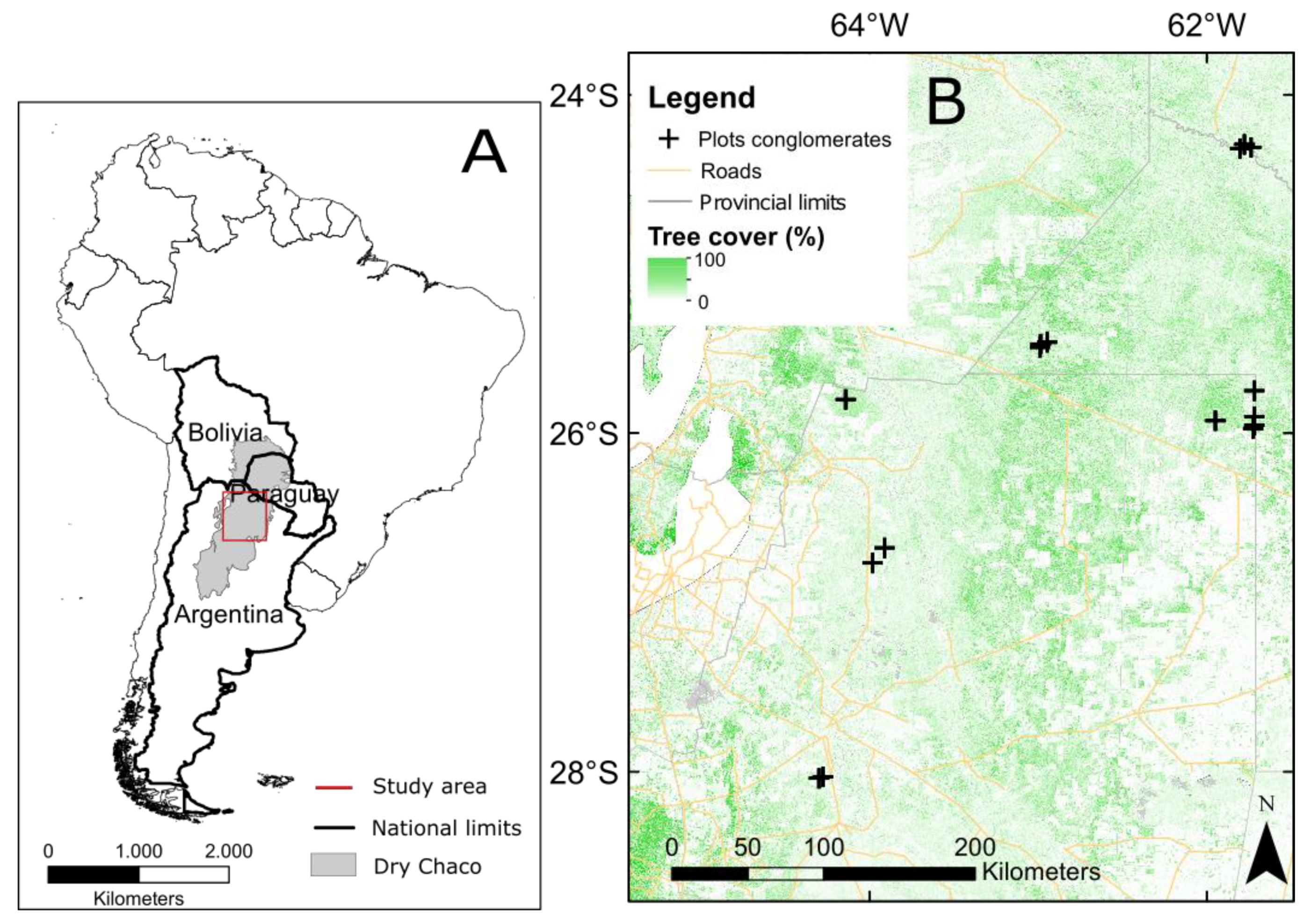
2.1. Study Area
2.2. Forest Inventory Data
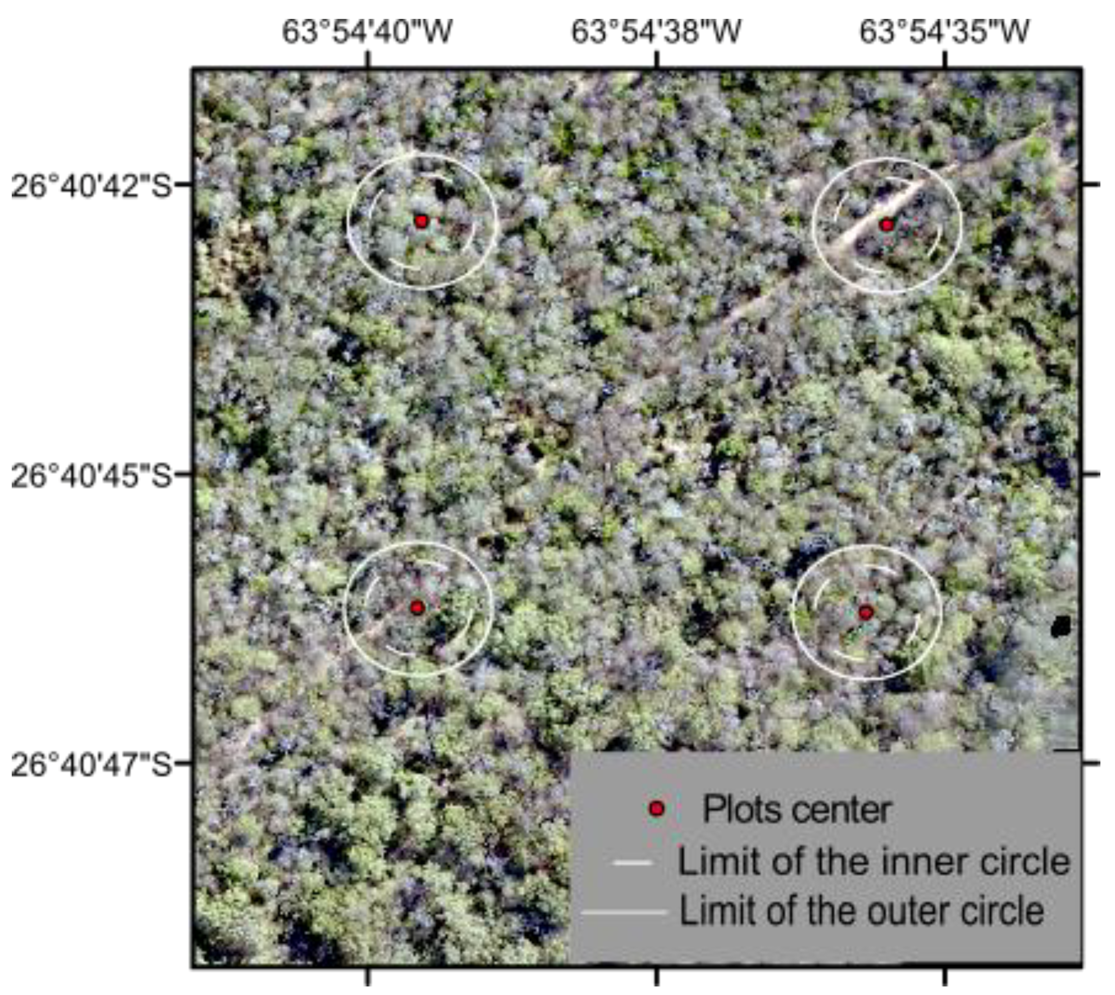
2.3. UAV Data Acquisition and SfM Image Processing
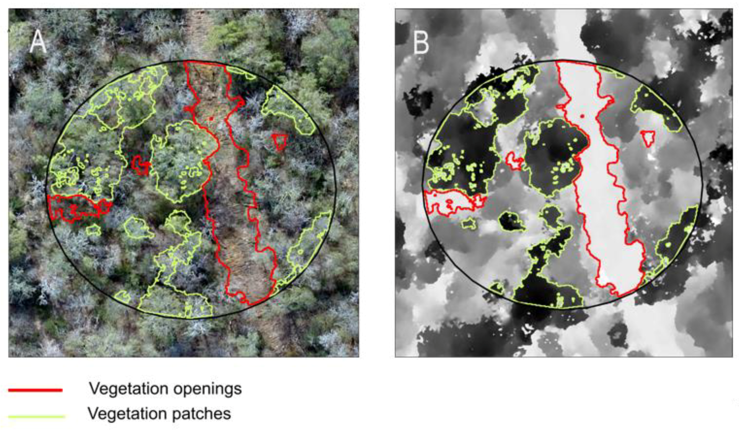
2.4. Image Processing and Variable Extraction
2.5. Data Analysis
3. Results
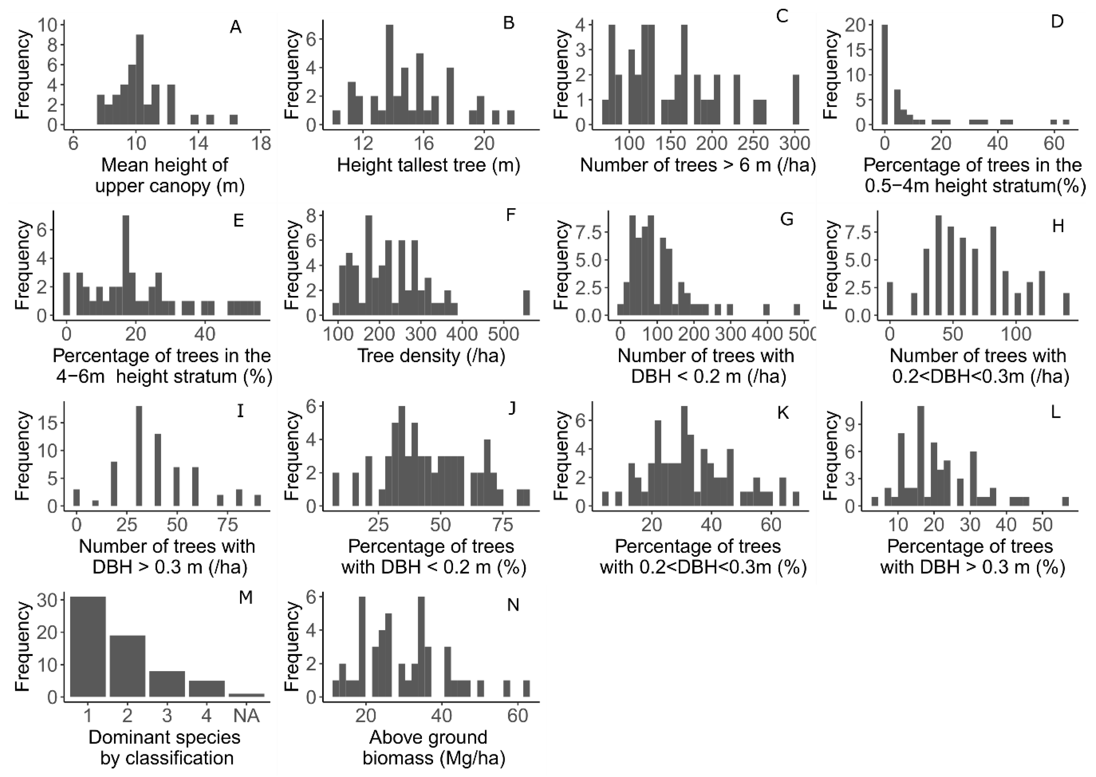
3.1. Forest Structure, Composition, and Function Based on Ground-Based Measures
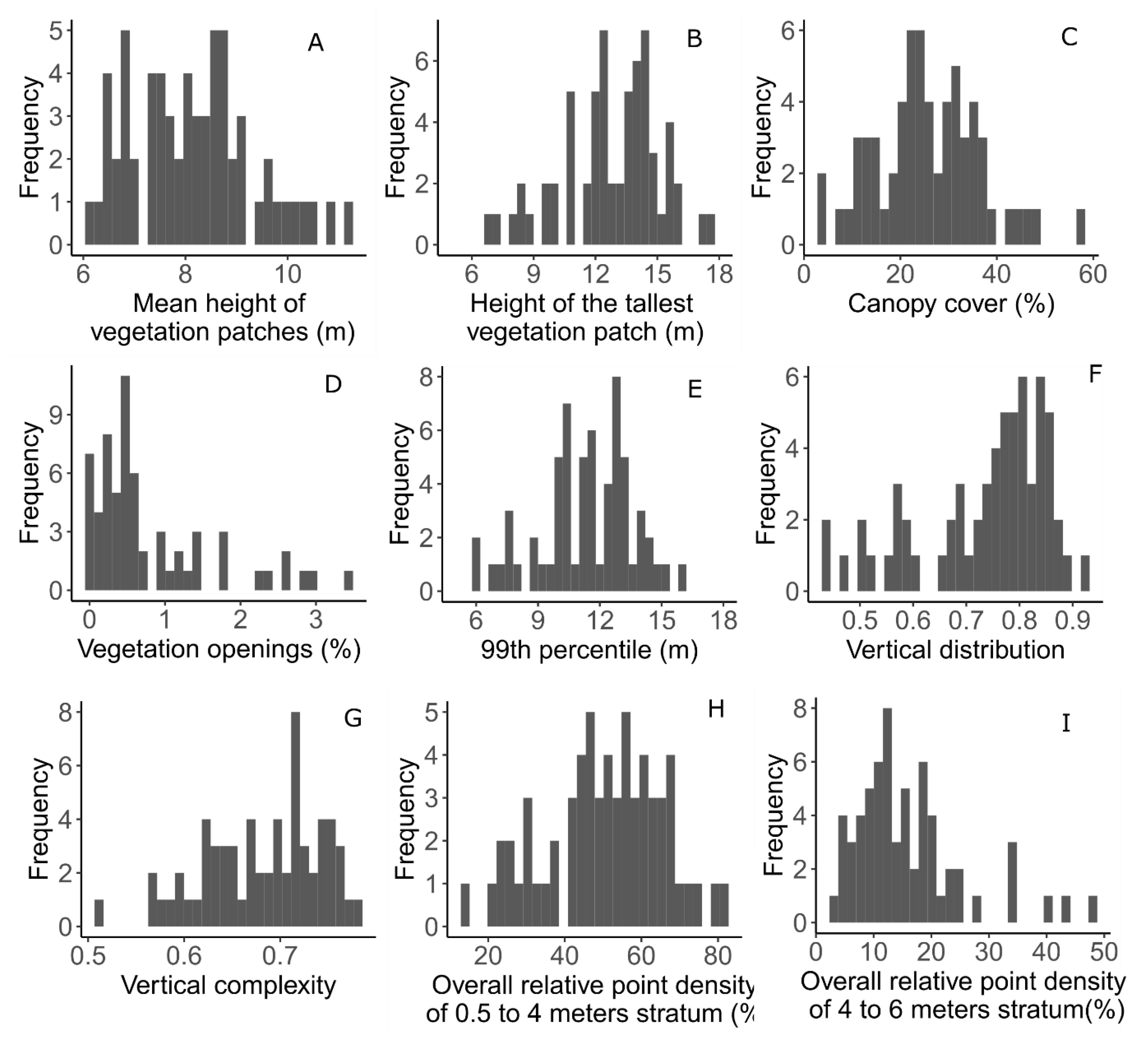
3.2. Horizontal and Vertical Forest Complexity Based on UAV-SfM Data
3.3. Performance of UAV-SfM Based Indicators on Forest Structure
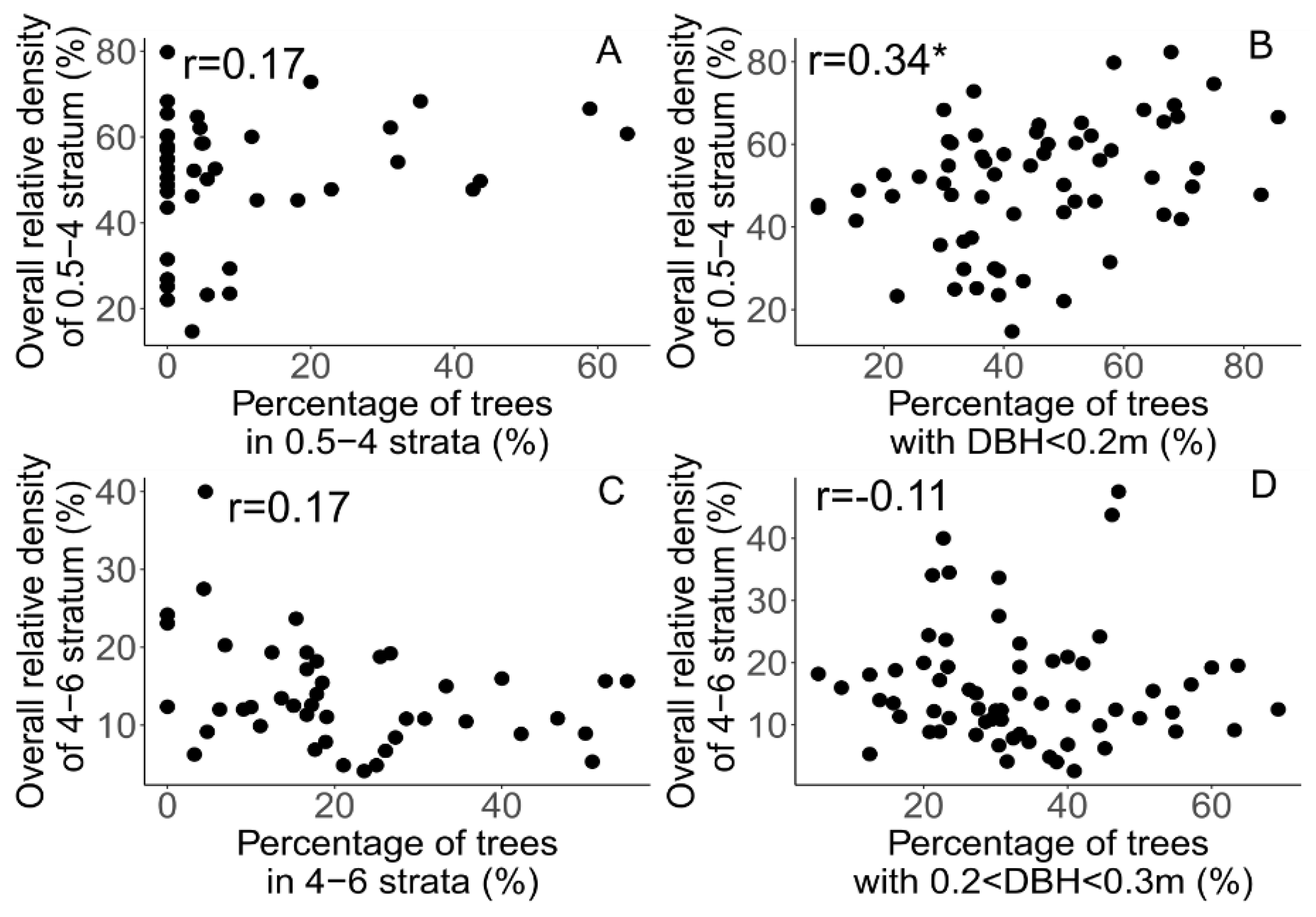
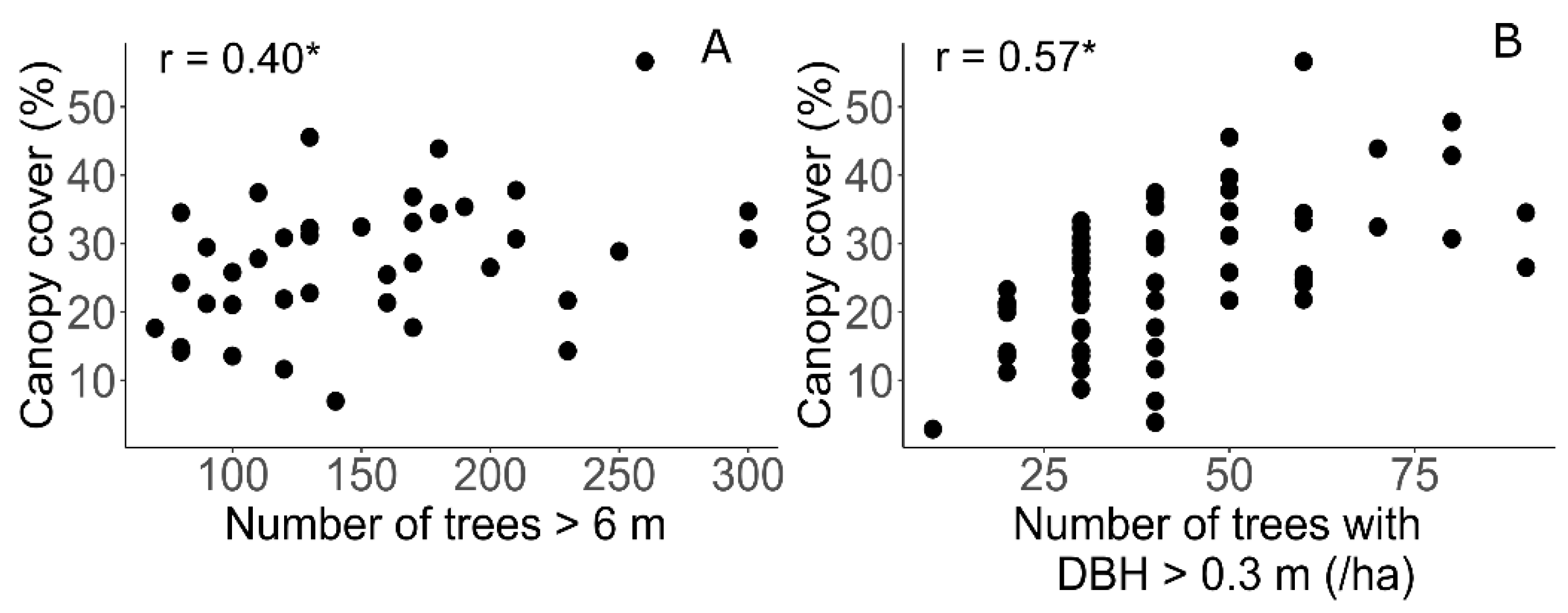
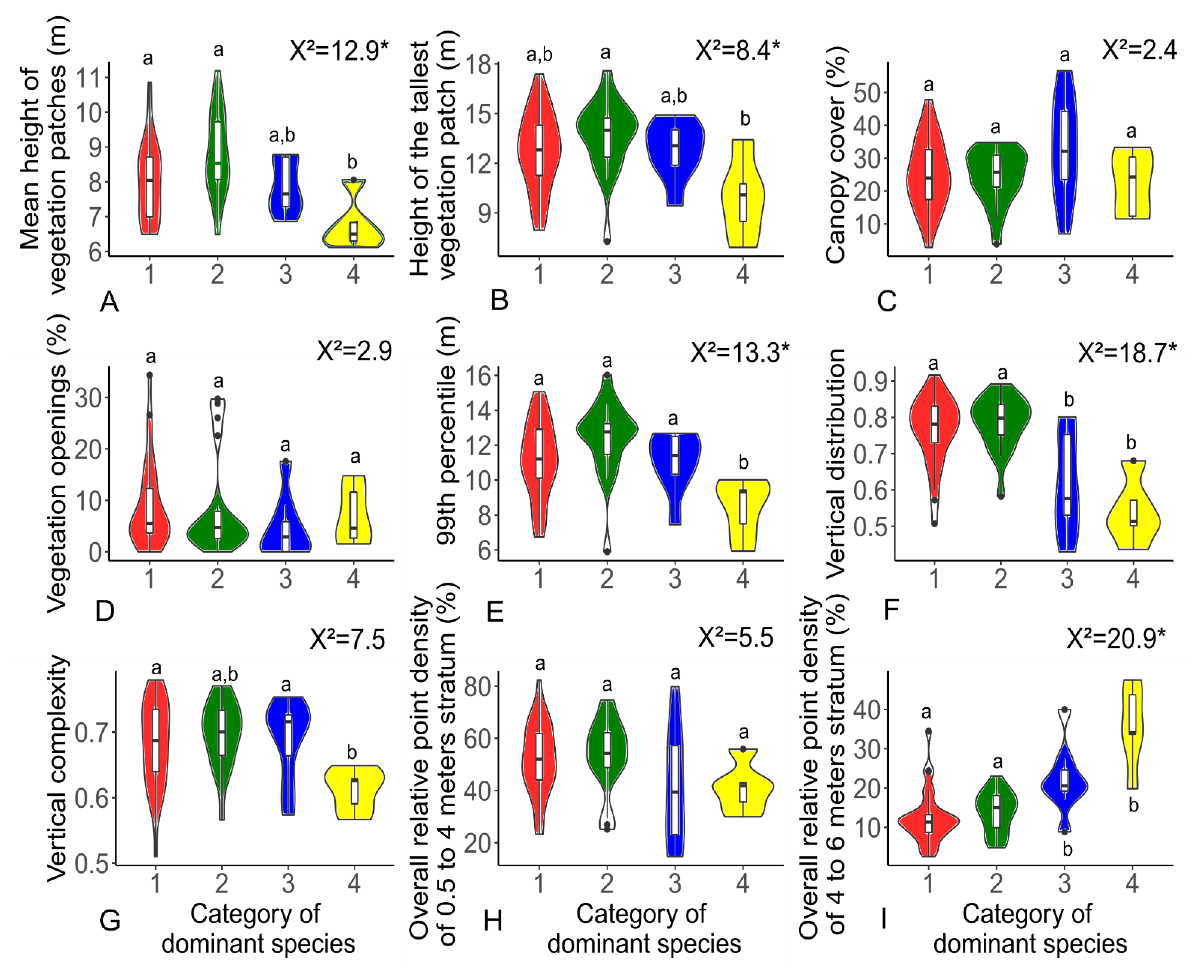
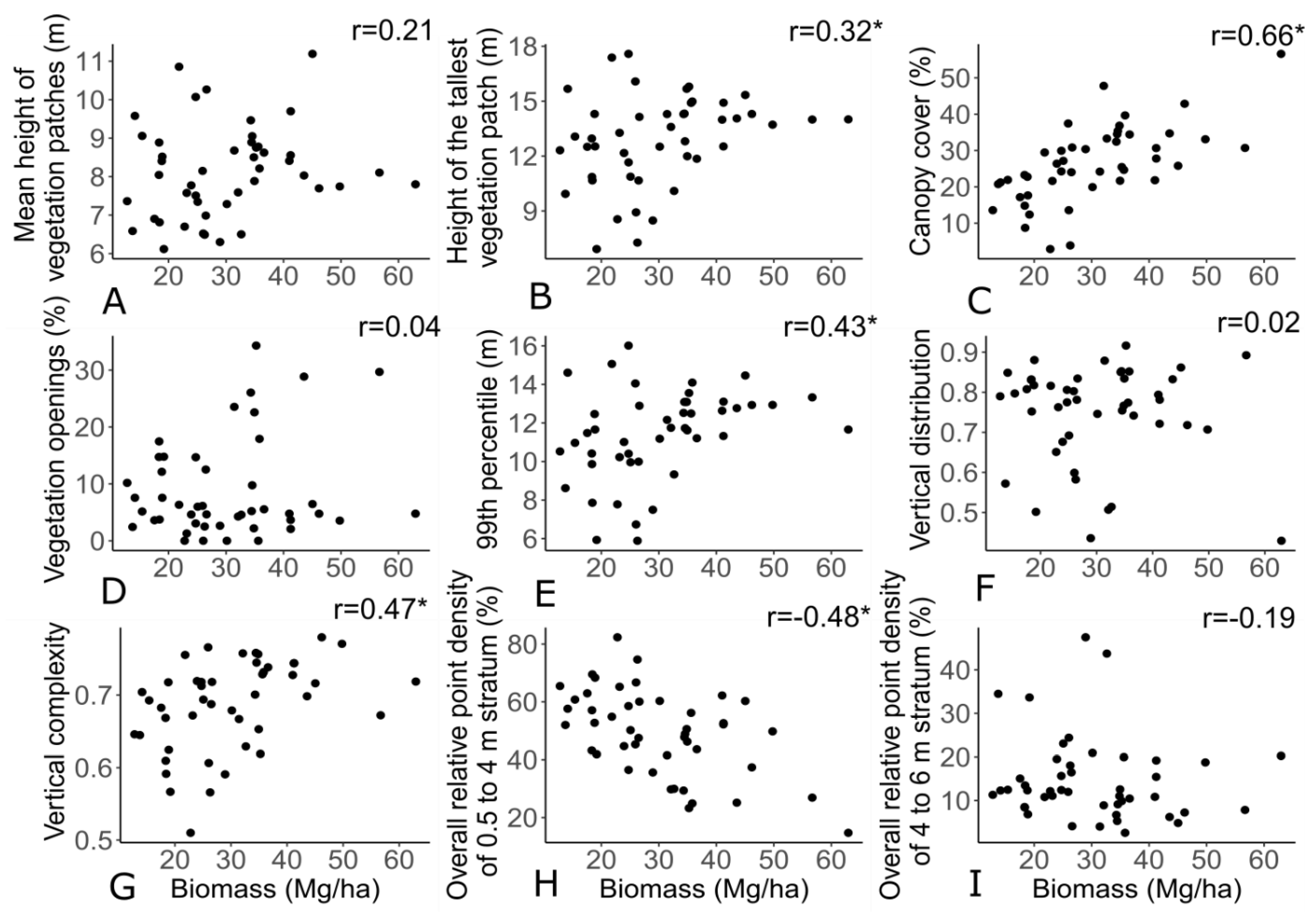
3.4. Relevance of UAV-SfM Based Indicators for Forest Composition and Function
4. Discussion
4.1. Forest Structural Indicators as Ecological Indicators
4.2. Horizontal Forest Complexity
4.2.1. Indicators of the Upper Canopy Structure
4.2.2. Canopy Cover
4.2.3. Vegetation Openings
4.3. Vertical Forest Complexity
4.3.1. Sub-Canopy and Shrub Stratum
4.3.2. Vertical Distribution and Vertical Complexity
5. Conclusions
Author Contributions
Funding
Acknowledgments
Conflicts of Interest
References
- Potapov, P.; Hansen, M.C.; Laestadius, L.; Turubanova, S.; Yaroshenko, A.; Thies, C.; Smith, W.; Zhuravleva, I.; Komarova, A.; Minnemeyer, S.; et al. The Last Frontiers of Wilderness: Tracking Loss of Intact Forest Landscapes from 2000 to 2013. Sci. Adv. 2017, 3, e1600821. [Google Scholar] [CrossRef] [PubMed] [Green Version]
- Watson, J.E.M.; Evans, T.; Venter, O.; Williams, B.; Tulloch, A.; Stewart, C.; Thompson, I.; Ray, J.C.; Murray, K.; Salazar, A.; et al. The Exceptional Value of Intact Forest Ecosystems. Nat. Ecol. Evol. 2018, 2, 599–610. [Google Scholar] [CrossRef] [PubMed]
- Balthazar, V.; Vanacker, V.; Molina, A.; Lambin, E.F. Impacts of Forest Cover Change on Ecosystem Services in High Andean Mountains. Ecol. Indic. 2015, 48, 63–75. [Google Scholar] [CrossRef]
- Venter, O.; Sanderson, E.W.; Magrach, A.; Allan, J.R.; Beher, J.; Jones, K.R.; Possingham, H.P.; Laurance, W.F.; Wood, P.; Fekete, B.M.; et al. Sixteen Years of Change in the Global Terrestrial Human Footprint and Implications for Biodiversity Conservation. Nat. Commun. 2016, 7, 1–11. [Google Scholar] [CrossRef] [PubMed] [Green Version]
- Piperno, D.R.; McMichael, C.N.H.; Bush, M.B. Finding Forest Management in Prehistoric Amazonia. Anthropocene 2019, 26, 100211. [Google Scholar] [CrossRef]
- Iglhaut, J.; Cabo, C.; Puliti, S.; Piermattei, L.; O’Connor, J.; Rosette, J. Structure from Motion Photogrammetry in Forestry: A Review. Curr. For. Rep. 2019, 5, 155–168. [Google Scholar] [CrossRef] [Green Version]
- Apostol, B.; Petrila, M.; Lorenţ, A.; Ciceu, A.; Gancz, V.; Badea, O. Species Discrimination and Individual Tree Detection for Predicting Main Dendrometric Characteristics in Mixed Temperate Forests by Use of Airborne Laser Scanning and Ultra-High-Resolution Imagery. Sci. Total Environ. 2020, 698, 134074. [Google Scholar] [CrossRef]
- Westoby, M.J.; Brasington, J.; Glasser, N.F.; Hambrey, M.J.; Reynolds, J.M. “Structure-from-Motion” Photogrammetry: A Low-Cost, Effective Tool for Geoscience Applications. Geomorphology 2012, 179, 300–314. [Google Scholar] [CrossRef] [Green Version]
- Passalacqua, P.; Belmont, P.; Staley, D.M.; Simley, J.D.; Arrowsmith, J.R.; Bode, C.A.; Crosby, C.; DeLong, S.B.; Glenn, N.F.; Kelly, S.A.; et al. Analyzing High Resolution Topography for Advancing the Understanding of Mass and Energy Transfer through Landscapes: A Review. Earth-Sci. Rev. 2015, 148, 174–193. [Google Scholar] [CrossRef] [Green Version]
- Clapuyt, F.; Vanacker, V.; Van Oost, K. Reproducibility of UAV-Based Earth Topography Reconstructions Based on Structure-from-Motion Algorithms. Geomorphology 2016, 260, 4–15. [Google Scholar] [CrossRef]
- Clapuyt, F.; Vanacker, V.; Schlunegger, F.; Van Oost, K. Unravelling Earth Flow Dynamics with 3-D Time Series Derived from UAV-SfM Models. Earth Surf. Dyn. 2017, 5, 791–806. [Google Scholar] [CrossRef] [Green Version]
- Dandois, J.P.; Ellis, E.C. High Spatial Resolution Three-Dimensional Mapping of Vegetation Spectral Dynamics Using Computer Vision. Remote Sens. Environ. 2013, 136, 259–276. [Google Scholar] [CrossRef] [Green Version]
- Puliti, S.; Ørka, H.O.; Gobakken, T.; Næsset, E. Inventory of Small Forest Areas Using an Unmanned Aerial System. Remote Sens. 2015, 7, 9632–9654. [Google Scholar] [CrossRef] [Green Version]
- Tuominen, S.; Balazs, A.; Saari, H.; Pölönen, I.; Sarkeala, J.; Viitala, R. Unmanned Aerial System Imagery and Photogrammetric Canopy Height Data in Area-Based Estimation of Forest Variables. Silva Fenn. 2015, 49, 1–19. [Google Scholar] [CrossRef] [Green Version]
- Messinger, M.; Asner, G.P.; Silman, M. Rapid Assessments of Amazon Forest Structure and Biomass Using Small Unmanned Aerial Systems. Remote Sens. 2016, 8, 615. [Google Scholar] [CrossRef] [Green Version]
- Otero, V.; Van De Kerchove, R.; Satyanarayana, B.; Martínez-Espinosa, C.; Fisol, M.A.B.; Ibrahim, M.R.B.; Sulong, I.; Mohd-Lokman, H.; Lucas, R.; Dahdouh-Guebas, F. Managing Mangrove Forests from the Sky: Forest Inventory Using Field Data and Unmanned Aerial Vehicle (UAV) Imagery in the Matang Mangrove Forest Reserve, Peninsular Malaysia. For. Ecol. Manag. 2018, 411, 35–45. [Google Scholar] [CrossRef]
- Jayathunga, S.; Owari, T.; Tsuyuki, S. Evaluating the Performance of Photogrammetric Products Using Fixed-Wing UAV Imagery over a Mixed Conifer-Broadleaf Forest: Comparison with Airborne Laser Scanning. Remote Sens. 2018, 10, 187. [Google Scholar] [CrossRef] [Green Version]
- Jacobson, A.P.; Riggio, J.M.; Tait, A.E.M.; Baillie, J. Global Areas of Low Human Impact (‘Low Impact Areas’) and Fragmentation of the Natural World. Sci. Rep. 2019, 9, 1–13. [Google Scholar] [CrossRef]
- Goetz, S.J.; Steinberg, D.; Betts, M.G.; Holmes, R.T.; Doran, P.J.; Dubayah, R.; Hofton, M. Lidar Remote Sensing Variables Predict Breeding Habitat of a Neotropical Migrant Bird. Ecology 2010, 91, 1569–1576. [Google Scholar] [CrossRef]
- Goetz, S.; Steinberg, D.; Dubayah, R.; Blair, B. Laser Remote Sensing of Canopy Habitat Heterogeneity as a Predictor of Bird Species Richness in an Eastern Temperate Forest, USA. Remote Sens. Environ. 2007, 108, 254–263. [Google Scholar] [CrossRef]
- Martins, A.C.M.; Willig, M.R.; Presley, S.J.; Marinho-Filho, J. Effects of Forest Height and Vertical Complexity on Abundance and Biodiversity of Bats in Amazonia. For. Ecol. Manag. 2017, 391, 427–435. [Google Scholar] [CrossRef]
- McElhinny, C.; Gibbons, P.; Brack, C.; Bauhus, J. Forest and Woodland Stand Structural Complexity: Its Definition and Measurement. For. Ecol. Manag. 2005, 218, 1–24. [Google Scholar] [CrossRef]
- Bucher, E.H.; Huszar, P.C. Sustainable Management of the Gran Chaco of South America: Ecological Promise and Economic Constraints. J. Environ. Manag. 1999, 57, 99–108. [Google Scholar] [CrossRef]
- Gasparri, N.I.; Baldi, G. Regional Patterns and Controls of Biomass in Semiarid Woodlands: Lessons from the Northern Argentina Dry Chaco. Reg. Environ. Chang. 2013, 13, 1131–1144. [Google Scholar] [CrossRef]
- Cabrera, A. Regiones Fitogeográficas Argentinas; ACME: Buenos Aires, Argentina, 1976. [Google Scholar]
- Cuadra, D.E.; Golemba, F.E.; Vera, F.D. Explotación Forestal en el Chaco: Sectores Que Ganan y Ecosistemas Que Pierden. XV Encuentro Profesores en Geografia del Nord. 2014. Available online: https://hum.unne.edu.ar/revistas/geoweb/Geo26/archivos/congreso%20geografia/Exposiciones/Exposiciones%20Eje%201/Cuadra-Golanva-Vera_EJE1.pdf (accessed on 3 December 2020).
- Rueda, C.V.; Baldi, G.; Gasparri, I.; Jobbágy, E.G. Charcoal Production in the Argentine Dry Chaco: Where, How and Who? Energy Sustain. Dev. 2015, 27, 46–53. [Google Scholar] [CrossRef]
- Gasparri, N.I. The Transformation of Land-Use Competition in the Argentinean Dry Chaco between 1975 and 2015. In Land Use Competition; Springer: Cham, Switzerland, 2016; pp. 59–73. [Google Scholar] [CrossRef] [Green Version]
- Grau, H.R.; Torres, R.; Gasparri, N.I.; Blendinger, P.G.; Marinaro, S.; Macchi, L. Natural Grasslands in the Chaco. A Neglected Ecosystem under Threat by Agriculture Expansion and Forest-Oriented Conservation Policies. J. Arid Environ. 2015, 123, 40–46. [Google Scholar] [CrossRef]
- Adamoli, J.; Sennhauser, E.; Acero, J.M.; Rescia, A. Stress and Disturbance: Vegetation Dynamics in the Dry Chaco Region of Argentina. J. Biogeogr. 1990, 17, 491. [Google Scholar] [CrossRef]
- Baumann, M.; Levers, C.; Macchi, L.; Bluhm, H.; Waske, B.; Gasparri, N.I.; Kuemmerle, T. Mapping Continuous Fields of Tree and Shrub Cover across the Gran Chaco Using Landsat 8 and Sentinel-1 Data. Remote Sens. Environ. 2018, 216, 201–211. [Google Scholar] [CrossRef]
- Loto, D.E.; Gasparri, I.; Azcona, M.; García, S.; Spagarino, C. Estructura y Dinámica de Bosques de Palo Santo En El Chaco Seco. Ecol. Austral 2018, 28, 64–73. [Google Scholar] [CrossRef] [Green Version]
- INTI-CITEMA. Listado de Densidades Secas de Maderas. Buenos Aires (Argentina). November 2007. Available online: https://www.inti.gob.ar/publicaciones/descargac/365 (accessed on 3 December 2020).
- Chave, J.; Andalo, C.; Brown, S.; Cairns, M.A.; Chambers, J.Q.; Eamus, D.; Fölster, H.; Fromard, F.; Higuchi, N.; Kira, T.; et al. Tree Allometry and Improved Estimation of Carbon Stocks and Balance in Tropical Forests. Oecologia 2005, 145, 87–99. [Google Scholar] [CrossRef]
- Gasparri, N.I.; Grau, H.R.; Manghi, E. Carbon Pools and Emissions from Deforestation in Extra-Tropical Forests of Northern Argentina between 1900 and 2005. Ecosystems 2008, 11, 1247–1261. [Google Scholar] [CrossRef]
- Powell, P.A.; Nanni, A.S.; Názaro, M.G.; Loto, D.; Torres, R.; Gasparri, N.I. Characterization of Forest Carbon Stocks at the Landscape Scale in the Argentine Dry Chaco. For. Ecol. Manag. 2018, 424, 21–27. [Google Scholar] [CrossRef] [Green Version]
- de Casenave, J.L.; Pelotto, J.P.; Protomastro, J. Edge-Interior Differences in Vegetation Structure and Composition in a Chaco Semi-Arid Forest, Argentina. For. Ecol. Manag. 1995, 72, 61–69. [Google Scholar] [CrossRef]
- Prado, D.E. What Is the Gran Chaco Vegetation in South America? I. A Review. Contribution to the Study of Flora and Vegetation of the Chaco. V. Candollea 1993, 48, 145–172. [Google Scholar]
- Tálamo, A.; Caziani, S.M. Variation in Woody Vegetation among Sites with Different Disturbance Histories in the Argentine Chaco. For. Ecol. Manag. 2003, 184, 79–92. [Google Scholar] [CrossRef]
- Dandois, J.P.; Olano, M.; Ellis, E.C. Optimal Altitude, Overlap, and Weather Conditions for Computer Vision Uav Estimates of Forest Structure. Remote Sens. 2015, 7, 13895–13920. [Google Scholar] [CrossRef] [Green Version]
- Snavely, N.; Seitz, S.M.; Szeliski, R. Modeling the World from Internet Photo Collections. Int. J. Comput. Vis. 2008, 80, 189–210. [Google Scholar] [CrossRef] [Green Version]
- Verhoeven, G. Taking Computer Vision Aloft-Archaeological Three-Dimensional Reconstructions from Aerial Photographs with PhotoScan. Archaeol. Prospect. 2011, 18, 67–73. [Google Scholar] [CrossRef]
- St-Onge, B.; Audet, F.A.; Bégin, J. Characterizing the Height Structure and Composition of a Boreal Forest Using an Individual Tree Crown Approach Applied to Photogrammetric Point Clouds. Forests 2015, 6, 3899–3922. [Google Scholar] [CrossRef]
- Lim, Y.S.; La, P.H.; Park, J.S.; Lee, M.H.; Pyeon, M.W.; Kim, J.I. Calculation of Tree Height and Canopy Crown from Drone Images Using Segmentation. J. Korean Soc. Surv. Geod. Photogramm. Cartogr. 2015, 33, 605–613. [Google Scholar] [CrossRef] [Green Version]
- Guerra-Hernández, J.; González-Ferreiro, E.; Sarmento, A.; Silva, J.; Nunes, A.; Correia, A.C.; Fontes, L.; Tomé, M.; Díaz-Varela, R. Using High Resolution UAV Imagery to Estimate Tree Variables in Pinus Pinea Plantation in Portugal. For. Syst. 2016, 25. [Google Scholar] [CrossRef] [Green Version]
- Zellweger, F.; Braunisch, V.; Baltensweiler, A.; Bollmann, K. Forest Ecology and Management Remotely Sensed Forest Structural Complexity Predicts Multi Species Occurrence at the Landscape Scale. For. Ecol. Manag. 2013, 307, 303–312. [Google Scholar] [CrossRef]
- van Ewijk, K.Y.; Treitz, P.M.; Scott, N.A. Characterizing Forest Succession in Central Ontario Using Lidar-Derived Indices. Photogramm. Eng. Remote Sens. 2011, 77, 261–269. [Google Scholar] [CrossRef]
- Onaindia, M.; Dominguez, I.; Albizu, I.; Garbisu, C.; Amezaga, I. Vegetation Diversity and Vertical Structure as Indicators of Forest Disturbance. For. Ecol. Manage. 2004, 195, 341–354. [Google Scholar] [CrossRef]
- Campbell, M.J.; Dennison, P.E.; Hudak, A.T.; Parham, L.M.; Butler, B.W. Quantifying Understory Vegetation Density Using Small-Footprint Airborne Lidar. Remote Sens. Environ. 2018, 215, 330–342. [Google Scholar] [CrossRef]
- Dale, V.H.; Beyeler, S.C. Challenges in the Development and Use of Ecological Indicators. Ecol. Indic. 2001, 1, 3–10. [Google Scholar] [CrossRef] [Green Version]
- NOSS, R.F. Indicators for Monitoring Biodiversity: A Hierarchical Approach. Conserv. Biol. 1990, 4, 355–364. [Google Scholar] [CrossRef]
- Sperlich, M.; Kattenborn, T.; Koch, B.; Kattenborn, G. Potential of Unmanned Aerial Vehicle Based Photogrammetric Point Clouds for Automatic Single Tree Detection. Gemeinsame Tagung 2014 der DGfK, der DGPF, der GfGI und des GiN. 2014, Volume 23. Available online: http://www.geocopter.eu/wp-content/uploads/2014/04/Shortpaper-UAV-Single-tree-detection.pdf (accessed on 3 December 2020).
- Bergen, K.M.; Goetz, S.J.; Dubayah, R.O.; Henebry, G.M.; Hunsaker, C.T.; Imhoff, M.L.; Nelson, R.F.; Parker, G.G.; Radeloff, V.C. Remote Sensing of Vegetation 3-D Structure for Biodiversity and Habitat: Review and Implications for Lidar and Radar Spaceborne Missions. J. Geophys. Res. Biogeosci. 2009, 114, 1–13. [Google Scholar] [CrossRef] [Green Version]
- Giménez, A.M.; Moglia, J.G. Árboles del Chaco Argentino. Guía para el Reconocimiento Dendrológico; U.N. de Santiago del Estero-FCF: Santiago del Estero, Argentina, 2003. [Google Scholar]
- Ferrero, M.E.; Villalba, R. Potential of Schinopsis Lorentzii for Dendrochronological Studies in Subtropical Dry Chaco Forests of South America. Trees Struct. Funct. 2009, 23, 1275–1284. [Google Scholar] [CrossRef]
- Dandois, J.P.; Ellis, E.C. Remote Sensing of Vegetation Structure Using Computer Vision. Remote Sens. 2010, 2, 1157–1176. [Google Scholar] [CrossRef] [Green Version]
- Wang, Y.; Lehtomäki, M.; Liang, X.; Pyörälä, J.; Kukko, A.; Jaakkola, A.; Liu, J.; Feng, Z.; Chen, R.; Hyyppä, J. Is Field-Measured Tree Height as Reliable as Believed—A Comparison Study of Tree Height Estimates from Field Measurement, Airborne Laser Scanning and Terrestrial Laser Scanning in a Boreal Forest. ISPRS J. Photogramm. Remote Sens. 2019, 147, 132–145. [Google Scholar] [CrossRef]
- da Silva, G.F.; de A Curto, R.; Soares, C.P.B.; de C Piassi, L. Avaliação de Métodos de Medição de Altura Em Florestas Naturais. Rev. Arvore 2012, 36, 341–348. [Google Scholar] [CrossRef] [Green Version]
- Mascaro, J.; Detto, M.; Asner, G.P.; Muller-Landau, H.C. Evaluating Uncertainty in Mapping Forest Carbon with Airborne LiDAR. Remote Sens. Environ. 2011, 115, 3770–3774. [Google Scholar] [CrossRef]
- Lutz, J.A.; Furniss, T.J.; Johnson, D.J.; Davies, S.J.; Allen, D.; Alonso, A.; Anderson-Teixeira, K.J.; Andrade, A.; Baltzer, J.; Becker, K.M.L.; et al. Global Importance of Large-Diameter Trees. Glob. Ecol. Biogeogr. 2018, 27, 849–864. [Google Scholar] [CrossRef] [Green Version]
- Sasaki, N.; Putz, F.E. Critical Need for New Definitions of “Forest” and “Forest Degradation” in Global Climate Change Agreements. Conserv. Lett. 2009, 2, 226–232. [Google Scholar] [CrossRef]
- FAO. Global Forest Resources Assessment 2000—Main Report; FAO: Rome, Italy, 2001. [Google Scholar]
- Smith, M.-L.; Anderson, J.; Fladeland, M. Forest Canopy Structural Properties. In Field Measurements for Forest Carbon Monitoring; Springer: Dordrecht, The Netherlands, 2008; pp. 179–196. [Google Scholar] [CrossRef]
- Getzin, S.; Nuske, R.S.; Wiegand, K. Using Unmanned Aerial Vehicles (UAV) to Quantify Spatial Gap Patterns in Forests. Remote Sens. 2014, 6, 6988–7004. [Google Scholar] [CrossRef] [Green Version]
- Morales-Barquero, L.; Skutsch, M.; Jardel-Peláez, E.J.; Ghilardi, A.; Kleinn, C.; Healey, J.R. Operationalizing the Definition of Forest Degradation for REDD+, with Application to Mexico. Forests 2014, 5, 1653–1681. [Google Scholar] [CrossRef] [Green Version]
- Conti, G.; Gorné, L.D.; Zeballos, S.R.; Lipoma, M.L.; Gatica, G.; Kowaljow, E.; Whitworth-Hulse, J.I.; Cuchietti, A.; Poca, M.; Pestoni, S.; et al. Developing Allometric Models to Predict the Individual Aboveground Biomass of Shrubs Worldwide. Glob. Ecol. Biogeogr. 2019, 28, 961–975. [Google Scholar] [CrossRef]
- Wallace, L.; Lucieer, A.; Turner, D.; Vopěnka, P. Assessment of Forest Structure Using Two UAV Techniques: A Comparison of Airborne Laser Scanning and Structure from Motion (SfM) Point Clouds. Forests 2016, 7, 62. [Google Scholar] [CrossRef] [Green Version]


| Stand Element | Variable | Description | Unit | |
|---|---|---|---|---|
| STRUCTURE | Tree height | Mean height of upper canopy | Mean height of trees taller than 6 m | m |
| Height tallest tree | Height of the tallest tree | m | ||
| Number of trees > 6 m | ha−1 | |||
| Percentage of trees in 0.5–4 m height stratum | % | |||
| Percentage of trees in 4–6 m height stratum | % | |||
| Tree spacing | Tree density | ha−1 | ||
| Tree diameter at breast height (DBH) | Number of trees with DBH < 0.2 m | ha−1 | ||
| Number of trees with 0.2 < DBH < 0.3 m | ha−1 | |||
| Number of trees with DBH > 0.3 m | ha−1 | |||
| Percentage of trees with DBH < 0.2 m | % | |||
| Percentage of trees with 0.2 < DBH < 0.3m | % | |||
| Percentage of trees with DBH > 0.3 m | % | |||
| COMPOSITIO | Species | Classification based on dominant tree species | Cat 1: Aspidosperma quebracho-blanco, Schinopsis lorentzii, Bulnesia sarmientoi Cat 2: Zizyphus mistol Cat 3: Caesalpinia paraguariensis and Tabebuia nodosa Cat 4: colonizer or pioneer species, like Prosopis nigra | |
| FUNCTION | Tree diameter and species | Above ground biomass (AGB) | For trees with DBH < 0.6 m: For trees with DBH > 0.6 m: | Mg ha−1 |
| Camera model | Phantom 4 Pro camera |
| Lens model | FOV 84° (8.8 mm/24 mm) f/2.8–f/11 |
| Image resolution | 5472 × 3648 |
| Crop factor | 1 |
| Approximate sensor size | 24 mm |
| Pixel size | 2.41 × 2.41 μm |
| Shutter speed | 8–1/8000 s |
| ISO Range | 100–3200 |
| Mean f number | 2.8–11 |
| Flight velocity | 2 m s−1 |
| Flight height | 80–120 m |
| Ground sample distance | 21.8–45.3 mm |
| Number of pictures | 160–217 |
| Point cloud density | 212–437 pt m−2 |
| CHM resolution | 3.4–9.1 cm pix−1 |
| Horizontal absolute accuracy | 2.6 m |
| Data Source | Processing | Indicators | Units |
|---|---|---|---|
 Canopy Height Model |  Canopy patches | Mean height of vegetation patches Height of the tallest vegetation patch Canopy cover | m m % |
 Vegetation openings | Vegetation openings | % | |
 Vegetation point cloud |  Height distribution of the point cloud | Stratum independent: 99th percentile Vertical distribution Vertical complexity | m |
| Stratum dependent: Overall relative point density of 0.5 to 4 m stratum Overall relative point density of 4 to 6 m stratum | % % |
| Forest Structure | Data Source | Indicator | Description | Unit |
|---|---|---|---|---|
| Horizontal complexity | CHM (Vegetation data points) | Mean height of tree crown patches | Mean of the maximum heights of the tree crown patches | m |
| Height of the tallest vegetation patch | Maximum height of the tallest canopy patch | m | ||
| Canopy cover | % | |||
| CHM (ground data points) | Vegetation openings | % | ||
| Vertical complexity | 3D point cloud (Percentile based) | 99th percentile | Height of 99th percentile of vegetation point cloud | m |
| Vertical distribution | ||||
| Vertical complexity | where pi is the proportional abundance of points within the height bin i; and HB is the total number of height bins of 1 m | |||
| 3D point cloud (ORD based) | Overall relative point density of 0.5 to 4 m stratum | % | ||
| Overall relative point density of 4 to 6 m stratum | % |
| Average | S.D. | Min. | Max. | # of Plots | |
|---|---|---|---|---|---|
| Mean height of upper canopy | 10.3 | 1.8 | 7.5 | 16.1 | 40 |
| Height tallest tree | 15.2 | 2.7 | 10.2 | 21.7 | 40 |
| Number of trees > 6 m | 153.0 | 60.7 | 70.0 | 300.0 | 40 |
| Percentage of trees in 0.5–4 m height stratum | 10.4 | 16.5 | 0.0 | 64.1 | 40 |
| Percentage of trees in 4–6 height stratum | 21.2 | 14.9 | 6.2 | 55.0 | 40 |
| Tree density | 231.1 | 94.4 | 100 | 560 | 64 |
| Number of trees with DBH < 0.2 m | 107 | 86.8 | 0 | 480 | 64 |
| Number of trees with 0.2 < DBH < 0.3m | 60 | 29.9 | 20 | 140 | 64 |
| Number of trees with DBH > 0.3 m | 42 | 18.6 | 0 | 90 | 64 |
| Dominant species by classification | - | - | - | - | 64 |
| Above ground biomass (AGB) | 30.0 | 11.3 | 12.8 | 62.9 | 64 |
| Average | S.D. | Min. | Max. | # of Plots | |
|---|---|---|---|---|---|
| Mean height of vegetation patches | 8.1 | 1.2 | 6.1 | 11.2 | 64 |
| Height of the tallest vegetation patch | 12.8 | 2.4 | 6.9 | 17.6 | 64 |
| Canopy cover | 25.6 | 10.8 | 2.8 | 56.6 | 64 |
| Vegetation openings | 8.3 | 8.1 | 0.0 | 34.3 | 64 |
| 99th percentile | 11.3 | 2.2 | 5.9 | 16 | 64 |
| Vertical distribution | 0.7 | 0.1 | 0.4 | 0.9 | 64 |
| Vertical complexity | 0.7 | 0.1 | 0.5 | 0.8 | 64 |
| ORD of 0.5 to 4 m stratum | 50.2 | 15.2 | 14.7 | 82.3 | 64 |
| ORD of 4 to 6 m stratum | 15.9 | 9.5 | 2.6 | 47.5 | 64 |
Publisher’s Note: MDPI stays neutral with regard to jurisdictional claims in published maps and institutional affiliations. |
© 2020 by the authors. Licensee MDPI, Basel, Switzerland. This article is an open access article distributed under the terms and conditions of the Creative Commons Attribution (CC BY) license (http://creativecommons.org/licenses/by/4.0/).
Share and Cite
Gobbi, B.; Van Rompaey, A.; Loto, D.; Gasparri, I.; Vanacker, V. Comparing Forest Structural Attributes Derived from UAV-Based Point Clouds with Conventional Forest Inventories in the Dry Chaco. Remote Sens. 2020, 12, 4005. https://0-doi-org.brum.beds.ac.uk/10.3390/rs12234005
Gobbi B, Van Rompaey A, Loto D, Gasparri I, Vanacker V. Comparing Forest Structural Attributes Derived from UAV-Based Point Clouds with Conventional Forest Inventories in the Dry Chaco. Remote Sensing. 2020; 12(23):4005. https://0-doi-org.brum.beds.ac.uk/10.3390/rs12234005
Chicago/Turabian StyleGobbi, Beatriz, Anton Van Rompaey, Dante Loto, Ignacio Gasparri, and Veerle Vanacker. 2020. "Comparing Forest Structural Attributes Derived from UAV-Based Point Clouds with Conventional Forest Inventories in the Dry Chaco" Remote Sensing 12, no. 23: 4005. https://0-doi-org.brum.beds.ac.uk/10.3390/rs12234005