Random Sample Fitting Method to Determine the Planetary Boundary Layer Height Using Satellite-Based Lidar Backscatter Profiles


1
Faculty of Information Engineering, China University of Geosciences, Wuhan 430074, China
2
Artificial Intelligence School, Wuchang University of Technology, 16, Jiangxia Avenue, Wuhan 430223, China
3
School of Geoscience and Info-Physics, Central South University, Changsha 410083, China
*
Author to whom correspondence should be addressed.
Remote Sens. 2020, 12(23), 4006; https://0-doi-org.brum.beds.ac.uk/10.3390/rs12234006
Submission received: 18 October 2020
/
Revised: 30 November 2020
/
Accepted: 5 December 2020
/
Published: 7 December 2020
(This article belongs to the Special Issue Remote Sensing of the Atmospheric Boundary Layer)
Abstract
:The planetary boundary layer height (PBLH) is the atmospheric region closest to the earth’s surface and has important implications on weather forecasting, air quality, and climate research. However, lidar-based methods traditionally used to determine PBLH—such as the ideal profile fitting method (IPF), maximum gradient method, and wavelet covariance transform—are not only heavily influenced by cloud layers, but also rely heavily on a low signal-to-noise ratio (SNR). Therefore, a random sample fitting (RANSAF) method was proposed for PBLH detection based on combining the random sampling consensus and IPF methods. According to radiosonde measurements, the testing of simulated and satellite-based signals shows that the proposed RANSAF method can reduce the effects of the cloud layer and significantly fluctuating noise on lidar-based PBLH detection better than traditional algorithms. The low PBLH bias derived by the RANSAF method indicates that the improved algorithm has a superior performance in measuring PBLH under a low SNR or when a cloud layer exists where the traditional methods are mostly ineffective. The RANSAF method has the potential to determine regional PBLH on the basis of satellite-based lidar backscatter profiles.
1. Introduction
The planetary boundary layer (PBL) is an atmospheric region near the Earth’s surface; it has a considerable impact on local and regional environmental conditions and is a key factor in weather forecasting models [1,2]. The entrainment layer at the top of the boundary layer (primarily an inversion layer) exerts a partial blocking effect on the dispersal of surface pollutants; this effect results in a high concentration of near-surface contaminants [3,4,5]. Therefore, the accurate determination of the planetary boundary layer height (PBLH) is an essential step in weather forecasting, climate change study, and air quality improvement [6,7].
Several technologies have been implemented to determine the PBLH, such as lidar, radiosonde [8,9,10,11], and microwave radiometers [12,13,14]. Radiosondes can accurately measure atmospheric parameters. However, the costly measurement device hanging below the balloon launches only twice a day (00:00 and 12:00 UTC) from a fixed station, which limits conventional radiosondes to retrieve PBLHs with high spatiotemporal coverage. Microwave radiometers provide temperature and humidity profiles with high temporal coverage but with limited precision, making the accurate estimation of the PBLH difficult. On the one hand, as an active detection tool, except for under effects of low clouds (below 900 m) or precipitation [14], ground-based lidar technology enables the low-cost measurement of PBLH with high time resolution for a fixed location.
On the other hand, satellite-based lidars, such as the Cloud-Aerosol Lidar with Orthogonal Polarization (CALIOP) aboard the Cloud-Aerosol Lidar and Infrared Pathfinder Satellite Observations (CALIPSO) satellite [15], have the potential to acquire PBLH characteristics over a large region with a temporal resolution of 16 days (including day and night) [16]. As one of the initial attempts to validate CALIOP-derived PBLHs, Kim, et al. [17] carried out an inter-comparison study between PBLHs from radiosondes and CALIOP measurements, showing high consistency between the instruments. Similarly, Liu, et al. [18] compared PBLHs from the CALIOP profiles with those from the European Center for Medium-Range Weather Forecasts reanalysis. Moreover, large biases in the seasonal and diurnal variations in PBLHs were observed among different methods such as radiosonde, ground-based lidar, and CALIOP observations [19]. Su, et al. [19] pointed out that the biases caused by low aerosol loading and elevated aerosol layers are difficult to be fundamentally solved.
The aerosol vertical distribution is strongly influenced by the thermal structure of the PBL. The aerosol loading within the PBL is higher than that in the free troposphere [20], which leads to the rapidly weakening changes in signal strength at the top of the boundary layer. Lidar-based PBLH detection algorithms search for strong decreases in the lidar signal with height. To date, the four widely used methods for lidar-based PBLH localization are ideal profile fitting (IPF) [21,22,23], maximum gradient (MGD) [7,24,25], maximum standard deviation (MSD) [19,26], and wavelet covariance transform (WCT) [27,28] methods. The IPF method is utilized to obtain the PBLH by fitting the lidar signal or particle backscatter coefficient to an idealized profile [21]. The MGD method determines the PBLH as the location of the maximum gradient of the lidar signal profile [7,24,25]. The WCT method analyzes the vertical gradients of aerosol and the fast temporal changes in the signal time series as a function of height [22,27,28]. Lidar-based PBLH localization depends on the rapidly weakening changes in the signal strength at the top of the boundary layer [27,29,30]. Unfortunately, similarly remarkable changes in the lidar signal can be caused by thick cloud layers and significantly fluctuating noise, especially for satellite-based lidar signals with extremely low signal-to-noise ratios (SNRs). Therefore, the four methods have been difficult to apply in the automatic and routine detection of the PBLH based on measured lidar signals due to their sensitivity to cloud layers and noises.
To weaken the adverse effects of strong backscatter layers and low SNR, a random sample fitting (RANSAF) method was proposed for lidar-based PBLH detection based on random sample consensus theory. Section 2 introduces the site and data used in this study. Section 3 describes theory of the RANSAF method. Then, the performance of the proposed RANSAF method is analyzed and compared by simulations and measured experiments in Section 4. Section 5 discusses the limitations of the RANSAF method.
2. Site and Data
2.1. Site
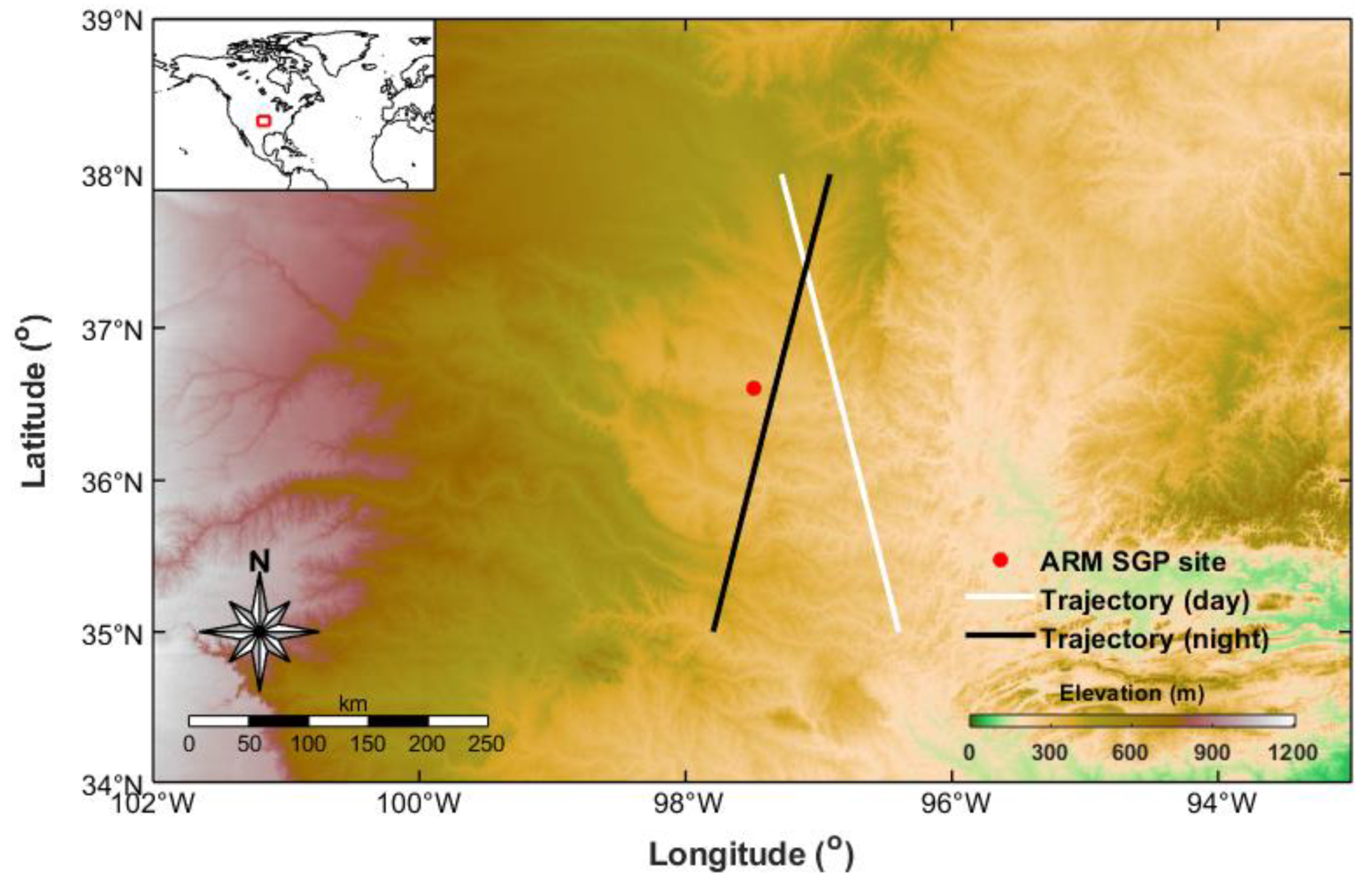
In this study, two types of data were applied, namely, satellite-based lidar backscatter profiles from CALIOP to test the RANSAF algorithm and radiosonde data to perform validation. The shared radiosonde data from the Atmospheric Radiation Measurement (ARM) Program were applied to investigate the performance of the proposed RANSAF method at the Southern Great Plains (SGP) central facility site near Lamont, Oklahoma (36.618°N, 97.498°W), as shown in Figure 1. The program was created in 1989 with funding from the U.S. Department of Energy to develop several highly instrumented ground stations to study cloud formation processes and their influence on radiative transfer [31].
2.2. Radiosonde
The balloon-borne sounding system launches four times per day (at approximately 05:30, 11:30, 17:30, and 23:30 local time (LT)) and provides in situ measurements (vertical profiles) of the thermodynamic state of the atmosphere and the wind speed and direction [32]. The method proposed by Liu and Liang [33] was adopted in this study as a reference value. The Liu–Liang method was used to determine the PBLH on the basis of the max gradient of a potential temperature profile. To distinguish the type of PBL, the classification method proposed by Liu and Liang [33] was also applied in this study. The PBLH can be classified as stable, neutral, or convective boundary layer by calculating the difference of potential temperature between the lowest fifth and second layers above the surface (i.e., an interval of 5-hPa) [34].
Moreover, synchronous measurements of temperature, pressure, relative humidity, and wind components were used to compute a bulk Richardson number to retrieve the PBLH. The bulk Richardson number, Rib, profile is calculated as
where θ is the potential temperature, g is the acceleration due to gravity, r is the height, r0 is the height of the surface, and μ and ν are the zonal and meridional wind components, respectively. The PBLH is defined by the height at which the condition Rib > Ribc, where Rib is the bulk Richardson number, is fulfilled. Zhang, et al. [35] pointed out that the best choices for Ribc are 0.22, 0.31, and 0.39 for strongly stable boundary layers, weakly stable boundary layers, and unstable boundary layers, respectively. The three critical values were taken for Ribc in different type of PBL, namely, stable (0.22), neutral (0.31), or convective boundary layer (0.39). Beyond this critical value of Ribc, the atmosphere can be considered decoupled from the PBL.
2.3. Atmospheric Emitted Radiance Interferometer
On account of the measured time difference between radiosonde and CALIPSO (>2 h), another ground-based instrument named atmospheric emitted radiance interferometer (AERI) was applied in this study to validate the results from the RANSAF method. The AERI can retrieve vertical profiles of temperature and water vapor with a temporal resolution of less than 15 min and an optimal vertical resolution of ~50 m by measuring the downwelling infrared radiance originating from the Earth’s atmosphere. AERI retrieval performance for temperature (water vapor) has been confirmed to be better than 1 K (5%) by validating with ARM radiosonde launched near SGP [36]. Therefore, the vertical profiles of temperature and water vapor retrieved from AERI were selected as the second reference value as a result of the measured time difference of AERI and CALIPSO is less than 10 min.
2.4. CALIPSO/CALIOP
CALIOP is an active sensor onboard the CALIPSO spacecraft. CALIOP is a nadir-looking, polarization-sensitive, elastic backscatter lidar instrument that uses a diode-pumped Nd:YAG laser that transmits at dual wavelengths of 532 and 1064 nm. CALIOP can provide vertical profiles of aerosols using the total backscatter radiation measured at the two wavelengths [37,38]. The overpass time of CALIOP/CALIPSO is near 02:30 and 13:40 LT. Therefore, the time difference between the CALIOP overpasses and radiosonde (AERI) measurements ranges from 2–3 h (less than 10 min). The minimum distance between the two instruments is approximately 20 km at nighttime and 50 km at daytime. The CALIPSO data at level 1 were used in this study to test the performance of our proposed RANSAF method for PBLH localization. The total attenuated backscatter (TAB) coefficient of a lidar is defined as [39]
where r is the altitude, which is above ground level; βp and βm refer to the backscatter coefficients of atmospheric particles and molecules, respectively; and , , and represent the two-way transmittances of atmospheric particles, molecules, and ozone, respectively. Atmospheric and ozone molecular density profiles can be obtained from meteorological data. Then, the backscatter coefficient under pure atmospheric conditions can be expressed as
Furthermore, the attenuated scatter ratio (ASR) can be derived as
The surface elevation at the laser footprint of CALIPSO was obtained from the GTOPO30 digital elevation map (DEM) and thus the reliability of the lidar surface elevations depends to some extent on the accuracy of the information recorded in GTOPO30. The absolute vertical accuracy of GTOPO30 varies by location according to the source data [40]. In general, vertical error was less than 100 m. Moreover, the elevation of the SGP site is 315 m, and the elevation of the CALIPSO laser footprint closest to the site is approximately 300 m. Therefore, the elevation correction of CALIPSO has less influence on the comparisons of PBLHs from different equipment.
In this study, four criterions were executed to screen the ASR profiles from CALIPSO. First, the minimum distance between CALIPSO footprint and the ARM site should be less than 60 km to weaken the adverse influence attributed to the measured distance difference between CALIPSO and radiosonde. If the minimum distance is 50 km, all daytime ASR profiles were screened out. Second, the CALIPSO signals should reach to the surface by the average ASR value from 0 to 1 km larger than 1 by reason of locating the PBLH is impossible if a satellite-based signal cannot be detected on the ground. Third, the temperature profiles derived from radiosonde and AERI were agreement with a high correlation coefficient (R > 0.9) and a small average difference (bias < 1 K) between the results from the two equipment. This criterion can reduce the disadvantageous influence caused by the measured time difference (>2 h) between CALIPSO and radiosonde. Fourth, daytime cases with relatively high PBLH (>1 km) were selected to weaken the adverse influence attributed to the measured distance differences between CALIPSO and radiosonde at daytime to some extent. The low distance differences (<20 km) had less influence on the nighttime comparisons between different sensors. In this study, the performance of the RANSAF method only validate by case analysis by reason of a small number of available ASR profiles up to the four criterions. The primary reason for limited ASR profiles is the low temporal resolution (16 day) of CALIPSO observation. Moreover, sometimes CALIPSO cannot capture the aerosol signals near the surface with the influence of impenetrable cloud layer or rain, which reduces the numbers of available profiles. Accidental equipment failures further reduce the number of available samples. Therefore, only representative ASR profiles that can demonstrate the improved performance of RANSAF method under effects of strong backscatter layers and low SNR conditions were selected in measured experiments.
To display the principle of the RANSAF method, an ASR profile with a cloud layer and noise was simulated. The extinction coefficients of molecules and ozone were calculated according to the US standard atmospheric model [41]. The aerosol (particle) extinction coefficients were three and one times of the molecular extinction coefficients at an altitude less and greater than 1 km, respectively. The extinction coefficient of cloud layers was simulated by three times of molecular extinction coefficients at an altitude of approximately 2 km. Therefore, the PBLH of this simulated ASR profile was 1 km. The ASR was added with Gaussian noise with a standard deviation of 1. Then, the simulated ASR was calculated by using Equations (2)–(4).
3. Methods
3.1. Ideal Profile Fitting (IPF) Method
Steyn, et al. [21] proposed the IPF method, which obtains the PBL parameters by fitting a lidar-derived backscatter profile to an idealized backscatter profile (B[r]). The IPF method is widely applied in lidar observations to determine the PBLH. The idealized backscatter profile (B[r]) can be expressed as [21,22]
where Bm is the mean mixed layer backscatter, Bµ is the mean backscatter in the air immediately above the mixed layer, rm is the mixed layer depth, and s is related to the thickness of the entrainment layer. The least squares fitting method is applied to minimize the root mean square deviation between the idealized backscatter (B[r]) and lidar-derived backscatter profiles. Thereafter, the four idealized backscatter profile parameters in Equation (5) can be determined. The thickness of the entrainment zone is equal to 2.77s, where s is the thickness of the layer in which the layer air and overlying air are mixed [21]. The satellite-based ASR was applied to estimate the PBLH (Equation (4)).
3.2. Random Sample Fitting (RANSAF) Method
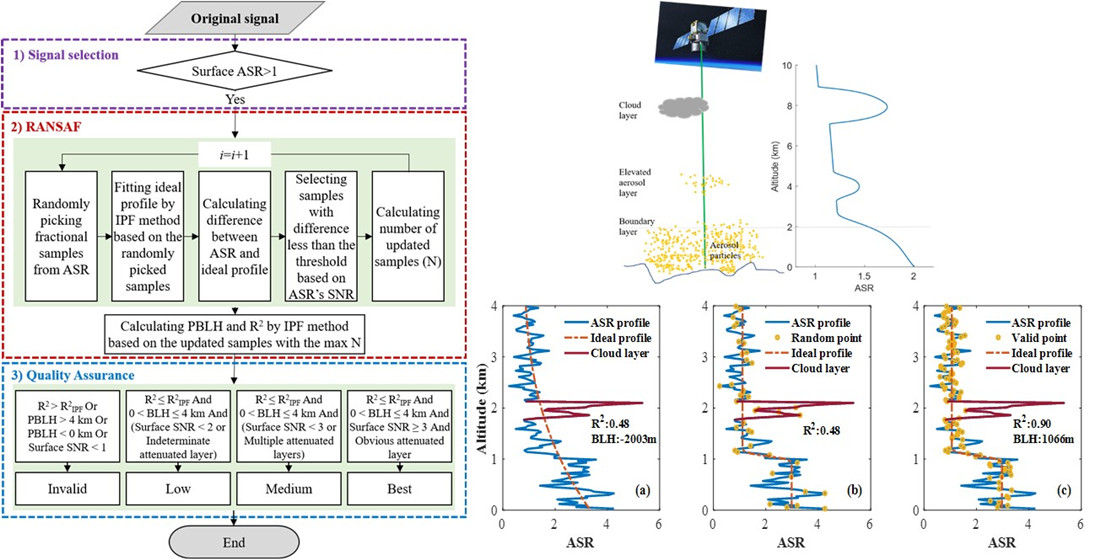
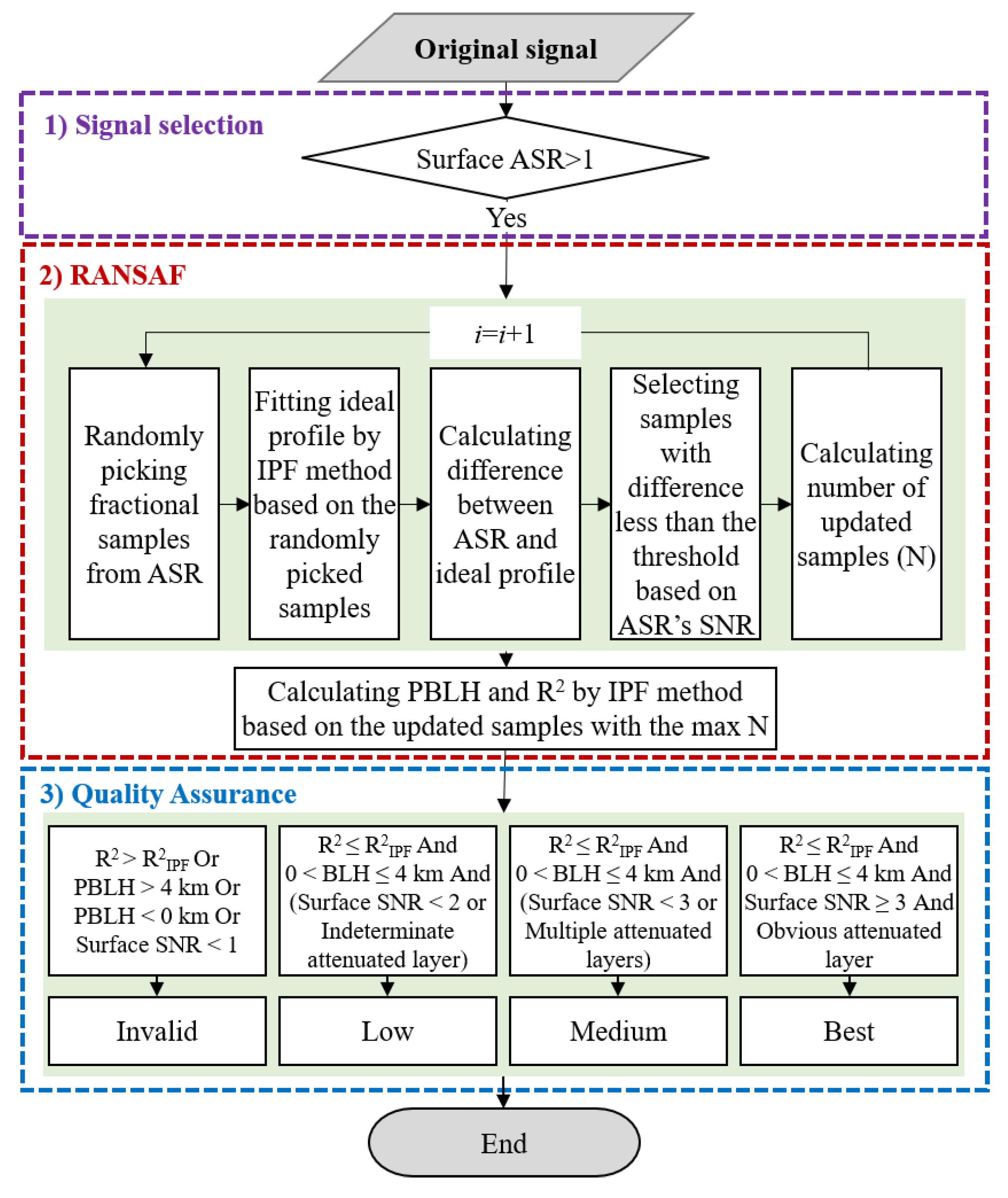
The random sample consensus method was proposed by Fischler and Bolles [42]. The method can interpret/smooth data containing a significant percentage of gross errors; thus, it is ideal for applications in automated image analysis where interpretation is based on data provided by error-prone feature detectors. The technique has been used for processing any noisy data set where there is a conviction that there is signal in there somewhere. Based on random sample consensus theory and the IPF method, the RANSAF method has been proposed for satellite-based PBLH measurements. Only the satellite-based signal that reaches the surface is processed during detection. Figure 2 presents a detailed flowchart of the RANSAF method.
The RANSAF method includes three steps:
- (1)
- Single selection
Notably, locating the PBLH is impossible if a satellite-based signal cannot be detected on the ground. Therefore, a threshold value (surface ASR > 1) is introduced to reflect the changes in aerosol loading from the surface to the top of the troposphere.
- (2)
- Random sample fitting
This step is crucial. Initially, fractional signal points (10–60% are recommended and 50% was used in this study, selected sample number is n) are selected randomly. A random permutation of the integers from 1 to the sample number of an ASR is generated. The ASR sample with the random integer’s permutation from 1 to n is selected. Then, an ideal profile [] is obtained by using the traditional IPF method based on the selected samples in the previous step. Next, the difference (diff) between the ASR and the ideal profile is calculated by applying the equation
where is ASR and the ideal profile at altitude . Subsequently, the updated samples (valid signals) with are reselected. A fixed threshold cannot be applied to various situations. A large fixed threshold results in the inability to filter out these valid signals, whereas a small fixed threshold leads to an insufficient number of valid signals to reflect true changes in signals. The threshold value () should reflect signal fluctuations caused by noise. Thus, it depends on the SNR of ASR. A proxy for the SNR, the standard deviation of ASR within the range of PBLH from 0 km to 4 km, can simply serve as the .
Finally, the number of updated samples (N) is calculated and saved. This step should be sufficiently repeated to ensure the validity of the results (100 iterations in this study). The optimal PBLH and ideal profile can be determined by using the IPF method according to the updated samples with the maximum N. The classical determination coefficient (R2) between ASR and the optimal ideal profile should be calculated to demonstrate the superiority of the RANSAF method.
- (3)
- Quality assurance
A mechanism of ‘quality assurance’ is set to quantify the uncertainty of PBLH detection, as random samples selected from the initial satellite-based signals do not always produce the correct/effective PBLHs according to the RANSAF method. The surface SNR plays a remarkable influence on the performance of the RANSAF method. The surface SNR was simply defined as a ratio of the average value and standard deviation of ASR near the surface
Then, the ‘quality assurance’ can be generated by different criteria. First, the determined PBLHs are invalid if the R2 from the RANSAF method is less than the determination coefficients () derived from the traditional IPF method or the results are beyond 0 to 4 km or SNR < 1 (extremely low SNR). Second, the quality of the determined PBLHs is low if the surface SNR < 2 (low SNR) or the ASR has an indeterminate attenuated layer (low aerosol loading). Third, the quality of the determined PBLHs is medium if the surface SNR < 3 (medium SNR) or the ASR has multiple attenuated layers (elevated aerosol layers). Fourth, the quality of the determined PBLHs is medium if the surface SNR ≥ 3 (high SNR) and the ASR has an obvious attenuated layer near the surface. Unfortunately, identifying automatically and correctly whether the ASR includes the indeterminate attenuated layer or multiple attenuated layers is difficult.
3.3. Other Traditional Methods
In this study, three other traditional methods—namely, MSD, MGD, and WCT—were utilized for comparison to demonstrate the performance of the RANSAF method.
3.3.1. MSD
When the CALIPSO signals from the instrument penetrate through an aerosol layer, they often become attenuated when they reach the bottom of the layer. This result generates a decline in the ASR below the top of the aerosol layer, which may also result in a local maximum of the ASR standard deviation [19].
where is ASR, r is altitude, and refers to the standard deviation of . PBLH can be determined where is a maximum.
3.3.2. MGD
The signal gradient can be calculated by
where r is altitude, and refers to the gradient of . The location with the maximum gradient (attenuation) can be regarded as the PBLH.
3.3.3. WCT
In the WCT method, Haar wavelet function h is defined as [43]
where r is altitude, b is called the ‘translation’ of the function where the function is centered, and a is called the ‘dilation’ of the function. Then, the covariance transform of Haar function is defined as
where is ASR, is the lower limit, and is the higher limit of the ASR profile. Value b at which reaches the local maximum with a coherent scale of a is usually considered the PBLH.
4. Results and Analysis
This section analyzes and compares the performance of the traditional methods and proposed RANSAF method for PBLH determination in simulated and measured experiments.
4.1. Simulated Experiment
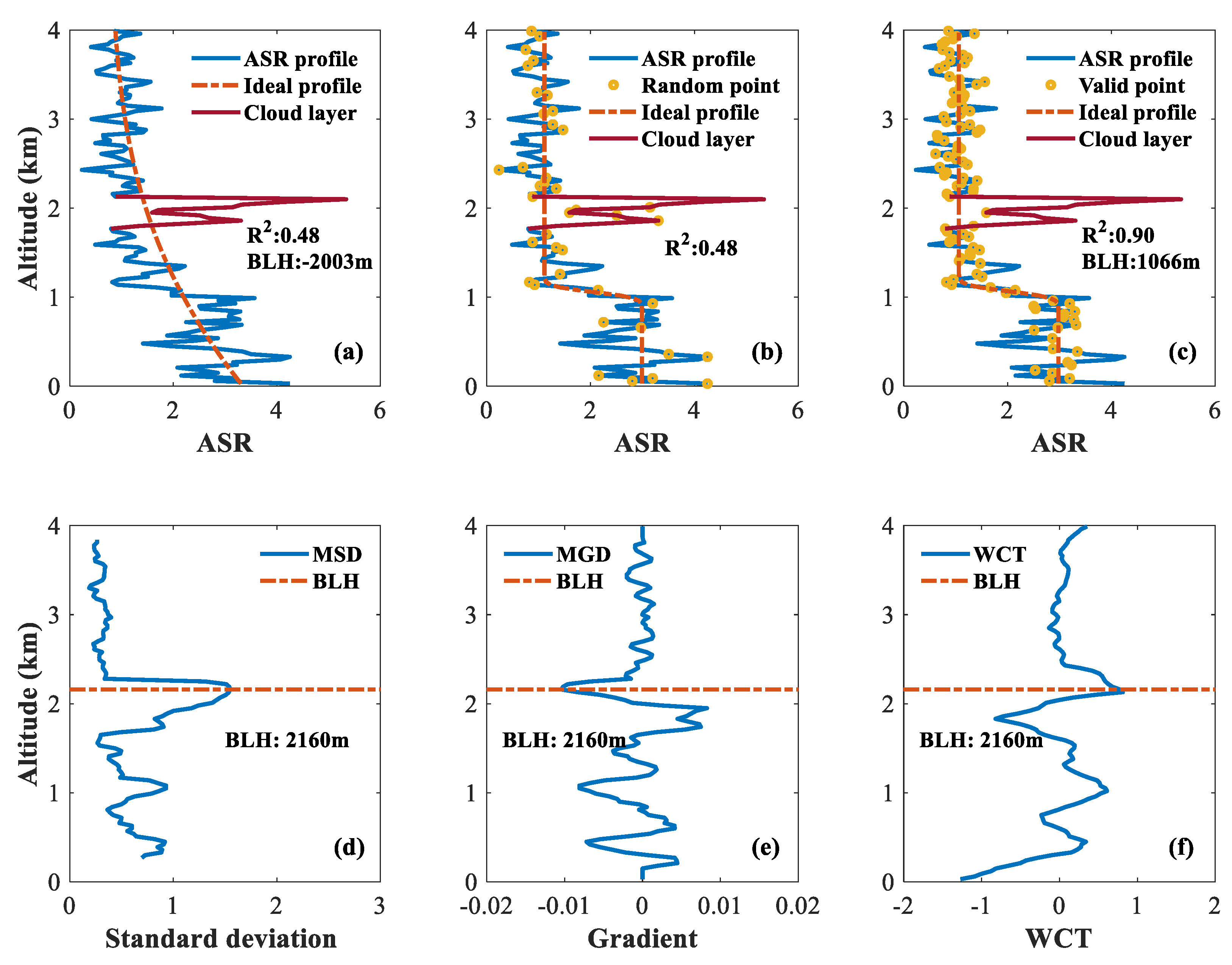
Figure 3 shows the estimation of PBLHs for the simulated ASR data with a reference PBLH of 1 km by using the IPF, MSD, MGD, WCT, and RANSAF methods. The blue solid line represents the ASR signal profile, the dashed orange line represents the ideal profile, and the red solid line represents a simulated cloud layer. Figure 3a shows the results of the PBLH calculation using the IPF method, including the values of the PBLH (−2003 m) and decision coefficient R2 (0.48). In principle, the PBLH cannot have a negative value. Therefore, the result indicates that traditional IPF method may be unsuitable for calculating the PBLH using a lidar signal with a thick cloud layer.
Figure 3b exhibits the ideal profile fitted by the randomly selected points (yellow circles) with an R2 of 0.48. Although some points were selected at the altitude with cloud layer, the fitted ideal profile can basically reflect the variations of the aerosol signal. Then, the differences [Θ(r)] between the ASR and the fitted ideal profile can be calculated by using Equation (6). Finally, the valid points can be screened by the differences [Θ(r)] and Θthr. Figure 3c shows the results of the PBLH calculation using the RANSAF method. The blue solid line refers to the ASR signal profile, the red dotted line is the ideal profile, and the yellow circles represent the valid sampling points. This figure shows that the calculation results for the fitting decision coefficient (R2) and PBLH are 0.90 and 1066 m, respectively. The reference PBLH of the simulated ASR profile was 1 km. Therefore, in the comparison between RANSAF and traditional IPF method, the higher R2 (0.90 versus 0.48) and lower bias (66 m versus −3003 m) suggest that the RANSAF method can be used to determine the more accurate PBLH in the presence of a thick cloud layer. Figure 3c–e show similar PBLH calculation results (2160 m) using the MSD, MGD, and WCT methods. Clearly, these methods incorrectly determine the PBLH at the cloud layer top. In this simulated experiment, these results suggest that the commonly used IPF, MSD, MGD, and WCT methods for calculating the PBLH can be easily affected by an optically thick layer. Fortunately, the proposed RANSAF method can effectively eliminate the influence of the cloud layer and return a valid PBLH.
4.2. Measured Experiment
4.2.1. Determining PBLH under Effects of Strong Backscatter Layers
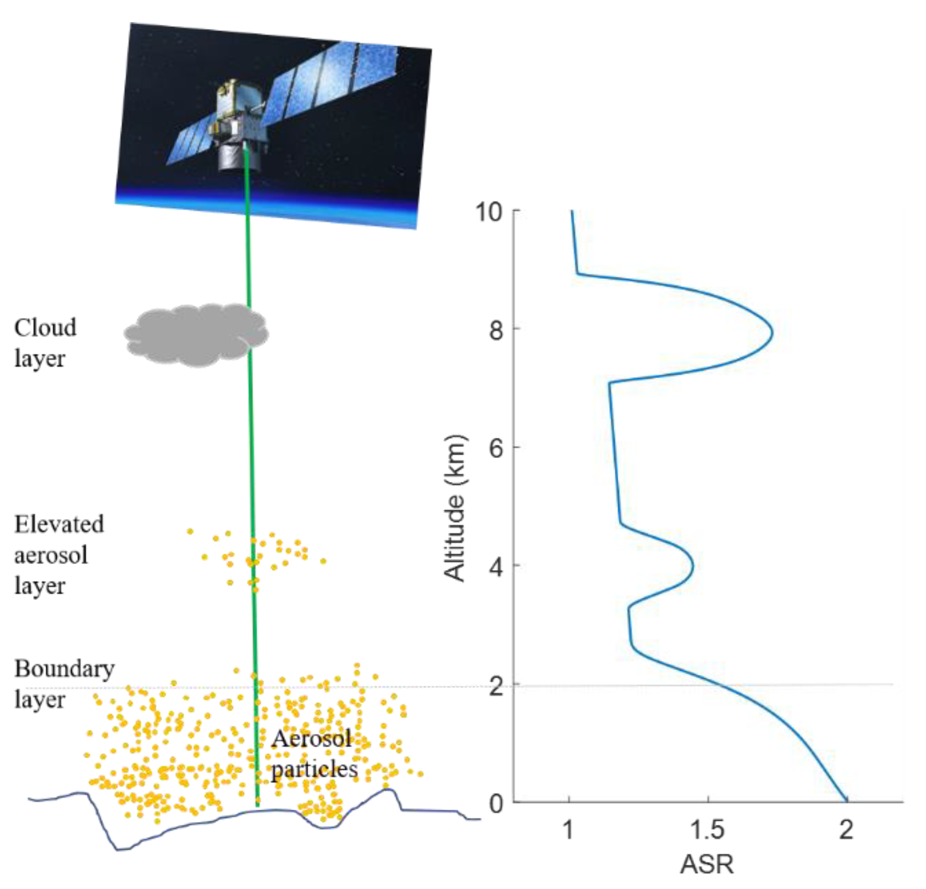
Strong backscatter layers, including cloud layers and elevated aerosol layers, are characterized by a steep increase in the ASR at the layer top, followed by a strong decrease in the signal with increasing layer penetration depth [27,44], as shown in Figure 4. These layers cause a strong increase between their tops and peaks, and a strong decrease between their peaks and bases in the backscattered signal. This type of strong decrease can cause these methods to mislocate the PBLH in areas with strong backscatter layers. Thus, the PBLH determination using these existing methods can be affected by strong backscatter layers, such as clouds and optically thick aerosols (e.g., mineral dust aerosol). Consequently, cases with strong backscatter layers were chosen to demonstrate whether the RANSAF method prevents the effects of strong backscatter layers and determines the correct PBLH.
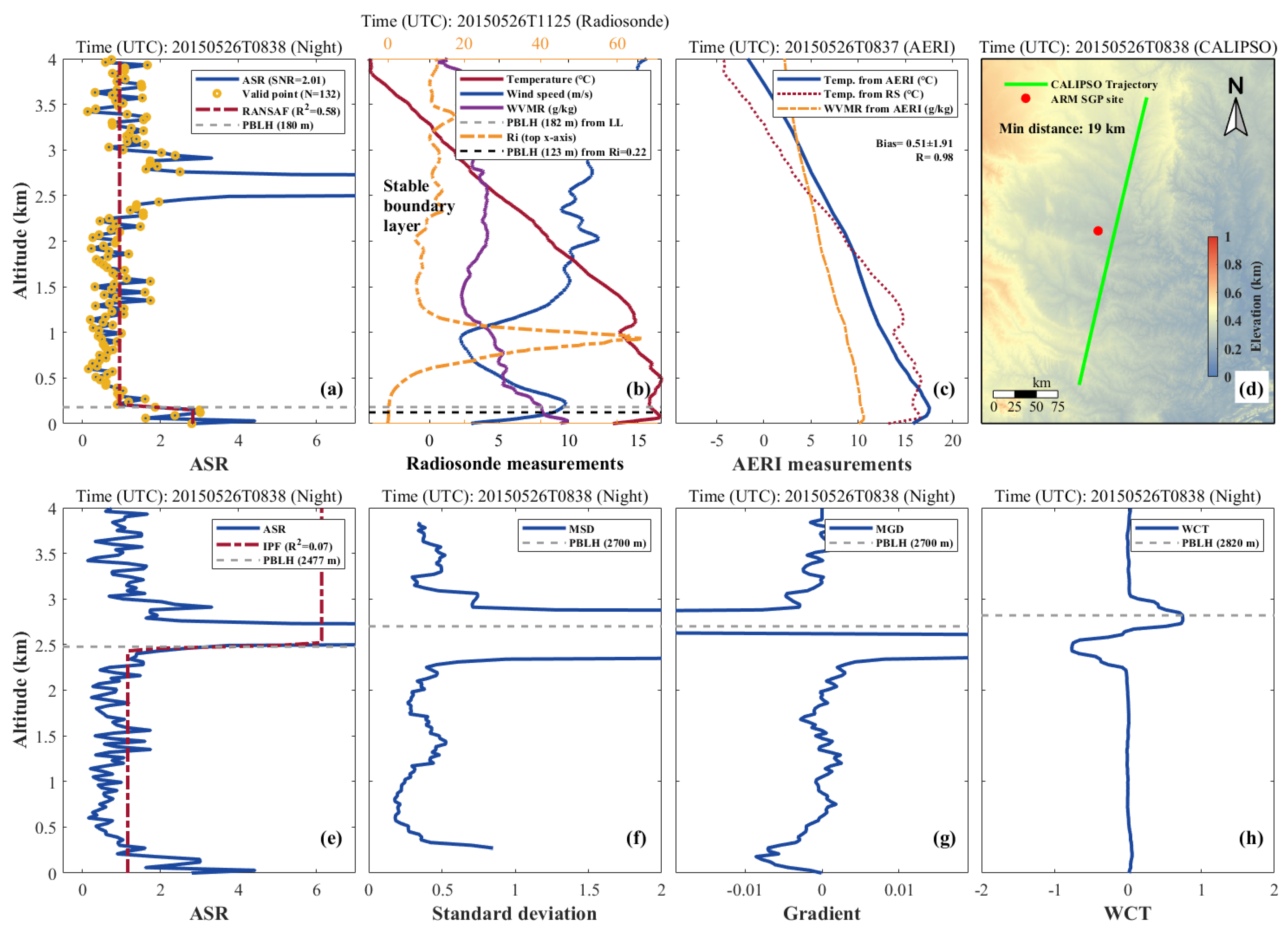
Figure 5 shows the PBLHs determined using the IPF, WCT, MSD, MGD, and RANSAF methods at 08:38:40 UTC (night) on 26 May 2015. This is a representative case under effects of strong backscatter layer. Figure 5a displays the PBLH (180 m) located using the proposed RANSAF method. The ideal fitting profile, marked by the red dotted line, is fitted by these randomly selected sampling points (marked as yellow circles) according to the RANSAF method with a high determination coefficient (R2 = 0.58). The result can be validated by radiosonde and AERI, as shown in Figure 5b. Comparatively, Figure 5e shows the calculated PBLH (2477 m) and the ideal fitting profile (orange dashed line) by using the IPF method with a small determination coefficient (R2 = 0.07). According to visual interpretation, the thick cloud layer, from 2400 m to 2800 m in this case, causes the traditional IPF method to return an erroneous result, that is, the cloud base height. The PBLH derived from the RANSAF method (180 m) is in agreement with that retrieved from the radiosonde, demonstrating that the PBLH derived from the proposed RANSAF method is more credible than that derived from the traditional IPF method when the ASR profile has an optically thick layer. To further illustrate the improvement of our proposed RANSAF method, other traditional algorithms—including the MSD, MGD, and WCT methods—were applied to determine the PBLH for the same case, as shown in Figure 5f–h. The basically consistent PBLH calculations (~2700 m) from the three traditional methods show similar results as those from the traditional IPF method (2477 m), indicating that these methods all incorrectly treat the cloud base height as the PBLH. This case suggests that the commonly used IPF, MSD, MGD, and WCT methods for calculating the PBLH can be easily affected by a thick cloud layer. If the top of the PBL differs from the location of the cloud layer, then the traditional methods will most likely directly associate the PBLH with the cloud layer height as a result of the similar attenuation change in the tops of cloud layers and PBL. Although these traditional methods identify the PBLH at the top of thick cloud layer for this case, the RANSAF method can distinguish and recognize the real position of the PBLH under cloudy conditions.
4.2.2. Determining PBLH under Low SNR Conditions
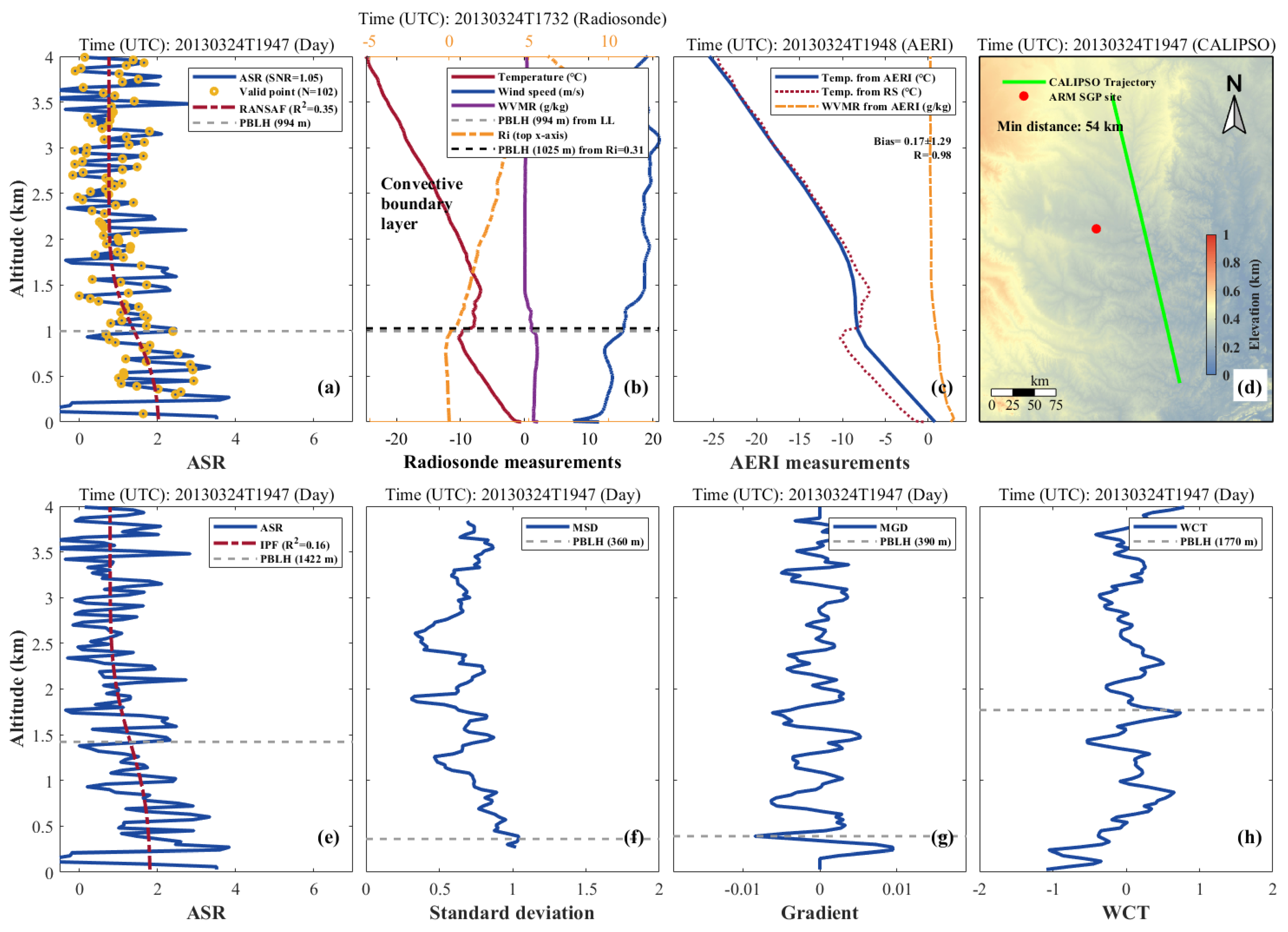
The SNR of the CALIOP signal is very low, especially during the day. Low surface SNR (< 2) signifies that the decrease in signal caused by the aerosol concentrations at the top of the BL was obliterated by the noise, making the determination of the PBLH under low SNR conditions difficult. Figure 6 displays a representative case under low SNR conditions. The reference profiles show this case is a convective boundary layer. The PBLH and fitting determination coefficient (R2) are 0.35 and 994 m, respectively. The high agreement (R = 0.98) of temperature profiles derived from the AERI and radiosonde suggest the similar PBLHs for the two different times. The reference PBLHs calculated by the radiosonde data at 17:32:00 (UTC) of the same day were 1025 m (Ri method) and 994 m (Liu and Liang method), as shown in Figure 6b. The PBLH determined by the RANSAF method has a small bias (<100 m) with reference value. Figure 6e shows the PBLH (1422 m) and ideal fitting profile marked with an orange dashed line, obtained by using the traditional IPF method with a fitting determination coefficient (R2 = 0.16). The high bias and low R2 indicates that the PBLH obtained from the traditional IPF method is suspect when the SNR of the lidar signal is low. Figure 6f–h show incorrect PBLHs of 360, 390, and 1770 m, which were calculated by using the MSD, MGD, and WCT methods, respectively. The large changes caused by the distinct noise fluctuations obliterate the variations contributed by the decreasing aerosol loading at the top of the PBL. Evidently, these methods incorrectly determine the PBLH as the height where the noise fluctuates greatly. In this experiment, the comparison suggests that these traditional methods (i.e., MSD, MGD, and WCT) are more susceptible than the RANSAF method to calculating the PBLH under low SNR conditions because they are sensitive to noise. To address this problem, denoising methods (e.g., time averaging or wavelet denoising method) can be applied in these satellite-based signals before PBLH detection.
4.2.3. Determining PBLHs from a CALIPSO Trajectory
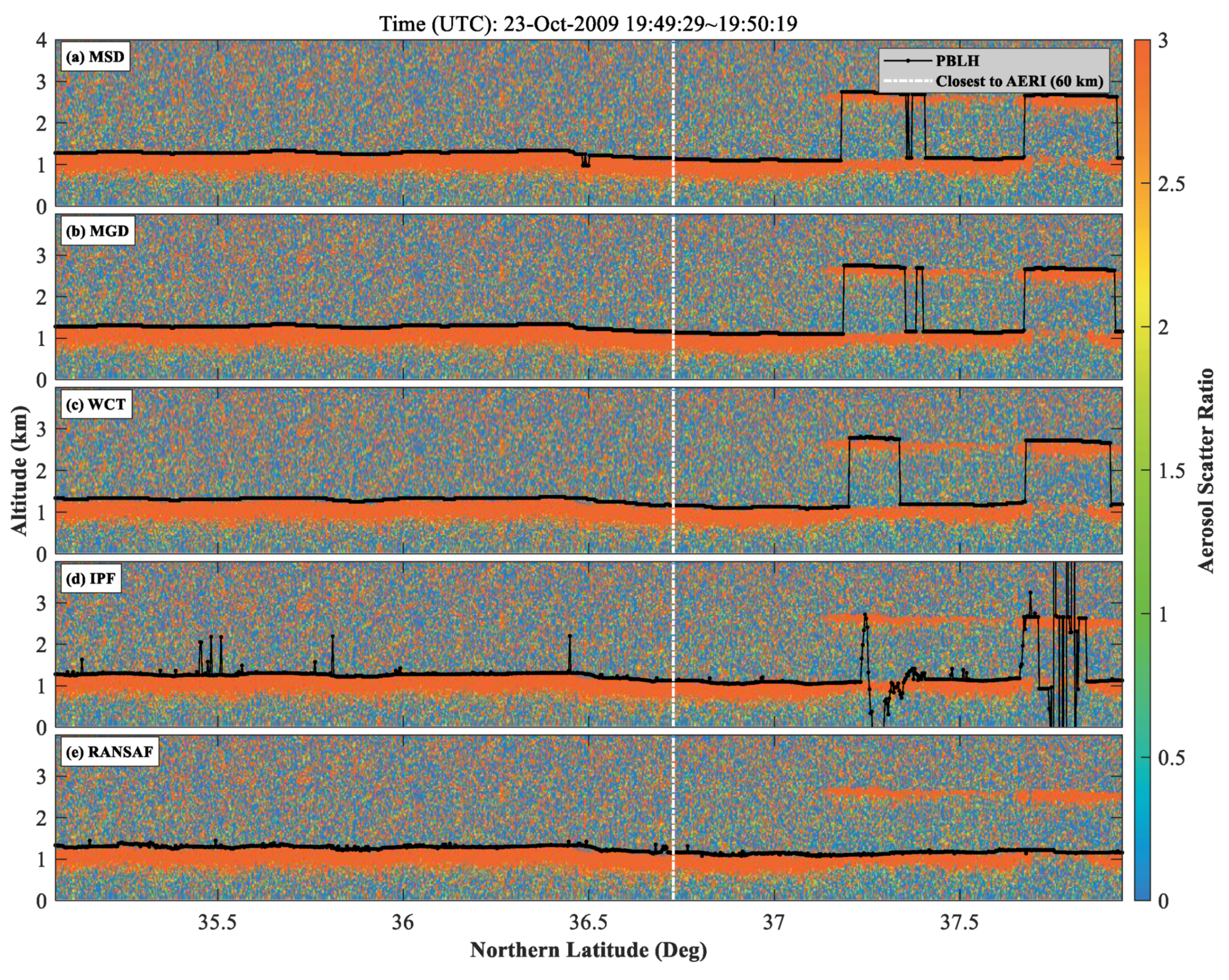
To validate the effectiveness of the RANSAF method in automatically extracting the PBLH from a long CALIPSO trajectory, we selected two time series of ASR from 19:49:29 to 19:50:19 on 23 October 2009 (UTC, daytime) and from 08:40:03 to 08:40:53 on 19 December 2009 (UTC, nighttime).
- (1)
- Case with strong backscatter layer
Figure 7 shows a comparison of the results of the MSD, MGD, WCT, IPF, and RANSAF methods based on the satellite-based ASR data from 19:49:29 to 19:50:19 on 23 October 2009 (UTC, daytime). This a representative case under effects of strong backscatter layers exist at 2.5 km from 37°N to 38°N. The reference PBLHs derived from radiosonde and AERI are 1149 m (Liu–Liang method) and 1169 m (Ri method), as shown in Figure 8. The reference profiles show this case is a convective boundary layer. The black dots represent the PBLHs estimated from different methods. A strong backscatter layer exists at approximately 2.5 km. The laser of the satellite-based lidar has difficulty penetrating strong backscatter layers in most cases, which results in the negligible signal near the surface. Some extremely weak signals that cannot be used for PBLH detection are removed by the first step of signal selection according to a threshold value (surface ASR > 1). In addition, the low SNRs of lidar signal are displayed near the surface. Remarkably, Figure 7a–c show that the MSD, MGD, and WCT methods incorrectly locate the cloud top as the top of the PBL. Figure 7d shows that the PBLHs derived by the IPF methods obviously change in a wide range (from 0 km to 4 km) as a result of the negative influence from the strong backscatter layer. Some incorrect results obtained by the traditional IPF method can be found in Figure 7d from 37.2°N and 38.0°N. Comparing with the reference value, the proposed RANSAF method demonstrates the lowest scatter along the observed track among the five methods. The strong backscatter layer has less influence on the RANSAF method to determine the PBLH on account of the random sampling mechanism.
- (2)
- Case with low SNRs
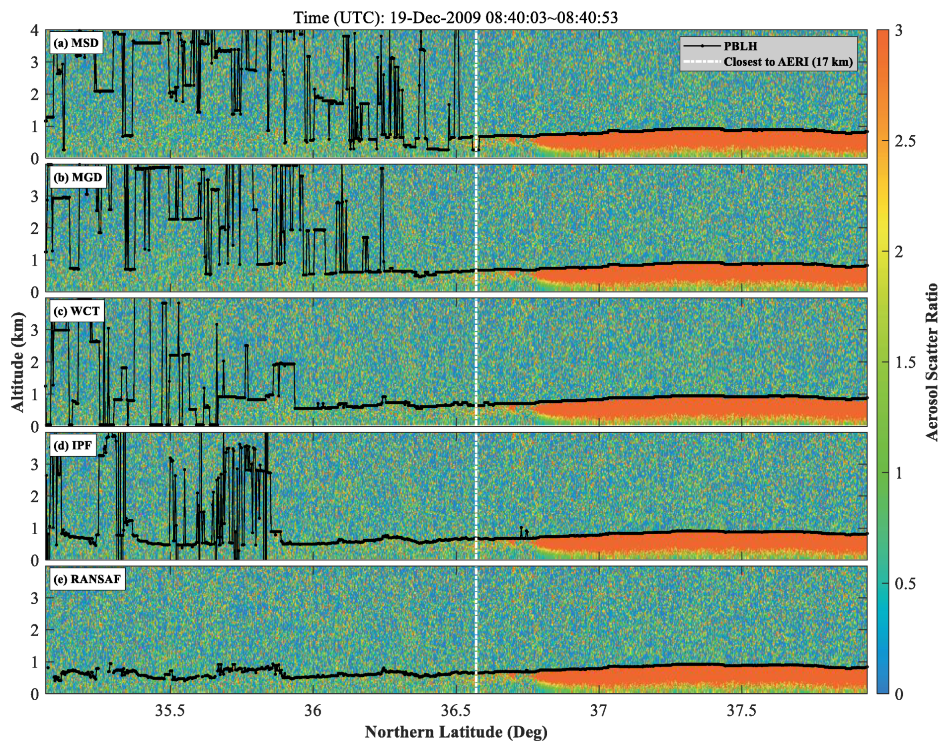
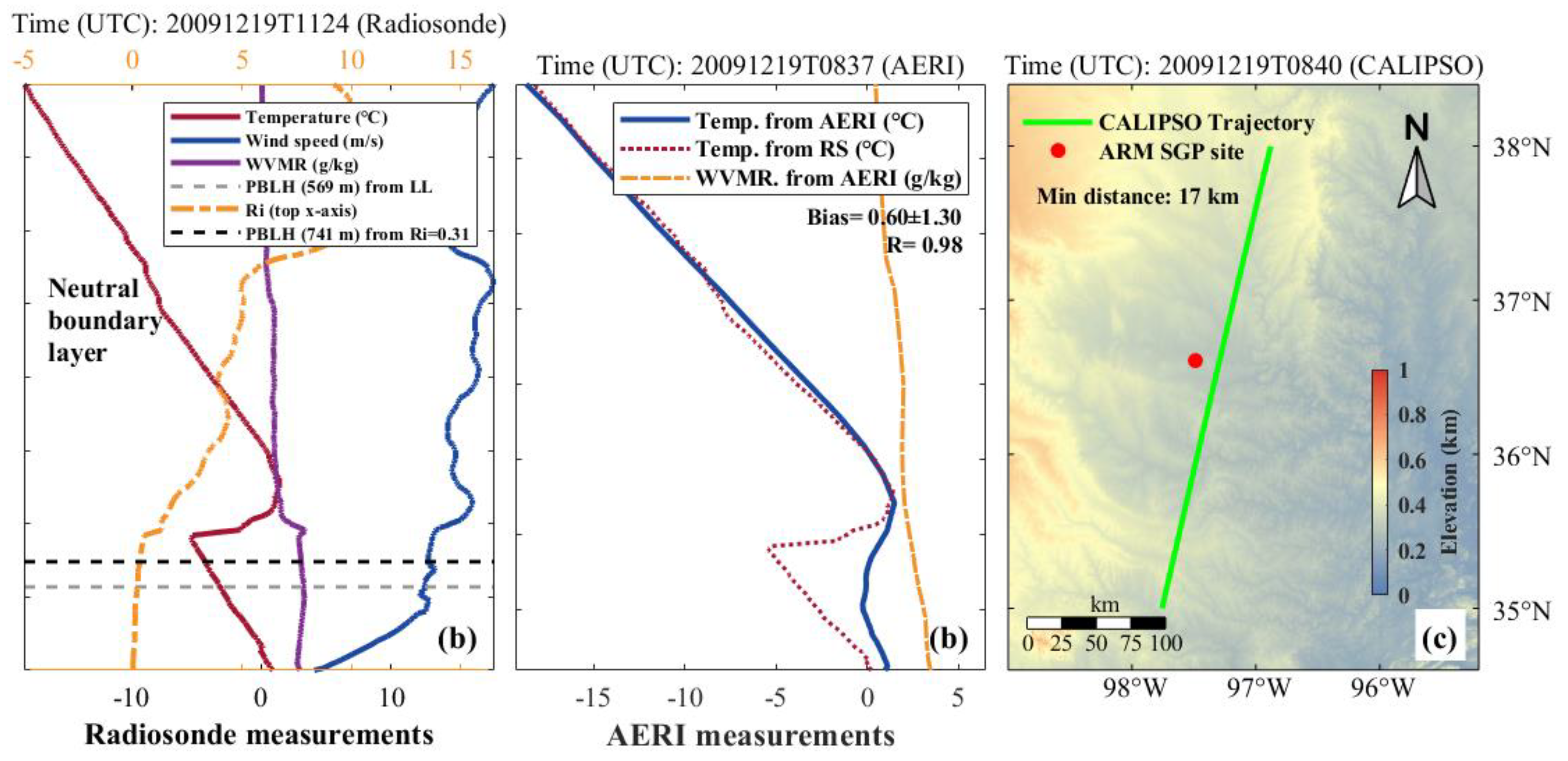
ASR (from 36.8°N to 38°N) with a high SNR and evident boundary layers (approximately 0.6 km) can be easily distinguished by visual interpretation (Figure 9). The reference PBLHs derived from radiosonde and AERI are 569 m (Liu–Liang method) and 741 m (Ri method), as shown in Figure 10. Consistent PBLHs can be derived by all five methods, as shown in Figure 9. The measured ASRs with low SNRs are shown from 35°N to 36.5°N. The low SNRs immensely disturb PBLH determination. Figure 9a–c show the strongly disordered results derived by using the MSD, MGD, and WCT methods. These results can be attributed to the sensitivity of the three traditional methods to noise disturbance. Moreover, comparing with the reference value from the radiosonde and AERI, distinctly incorrect PBLHs (above 4 km or less than 0 km) distributed from 35°N to 36°N were calculated by using the traditional IPF method as shown in Figure 9d. Many of the PBLHs determined by using the traditional IPF method are negative or larger than 4 km when the SNR is low. Comparatively, the RANSAF method can achieve more similar outcomes with the reference value than the other form traditional methods under low SNR condition, because the method can extract valid signal from raw signal mixed with considerable noise. Similarly, invalid results derived from the RANSAF method still exist in some measured cases with extremely low SNRs due to substantial noise that completely obscures the change in signal caused by aerosol loadings.
5. Discussion
The proposed RANSAF method does not always provide a correct solution in practical application. Increasing the number of iterations can evidently enhance the probability of obtaining an optimal solution. The drawback of this method is the longer operating time than those in traditional methods. In this study, 100 iterations were adopted in the experiments. In addition, the RANSAF cannot obtain a correct result under certain conditions, such as the presence of multiple attenuated layers and an indeterminate attenuated layer, which was discussed in the following sections.
5.1. Multiple Attenuated Layers
Figure 11 shows a case measured at 19:46:46 UTC (day) on 31 August 2007. The reference profiles show this case is a convectively unstable boundary layer. Multiple attenuated layers in this case can be observed at approximately 300 m, 1300 m, and 2500 m. This is a representative case with multiple attenuated layers. The reference value of the PBLHs derived from radiosonde are 1356 m from the Liu–Liang method and Ri method, which is in agreement with the result retrieved by using the RANSAF method (1284 m). Unfortunately, the proposed RANSAF method cannot always locate the correct top of the BL in multiple tests. The three attenuated locations, 300 m, 1300 m, and 2500 m are randomly treated as the output result. We assume that the three attenuated layers have a similar characteristic that results in a difficult determination by the proposed method. The traditional methods also fail to provide a solution in this situation.
5.2. Indeterminate Attenuated Layer
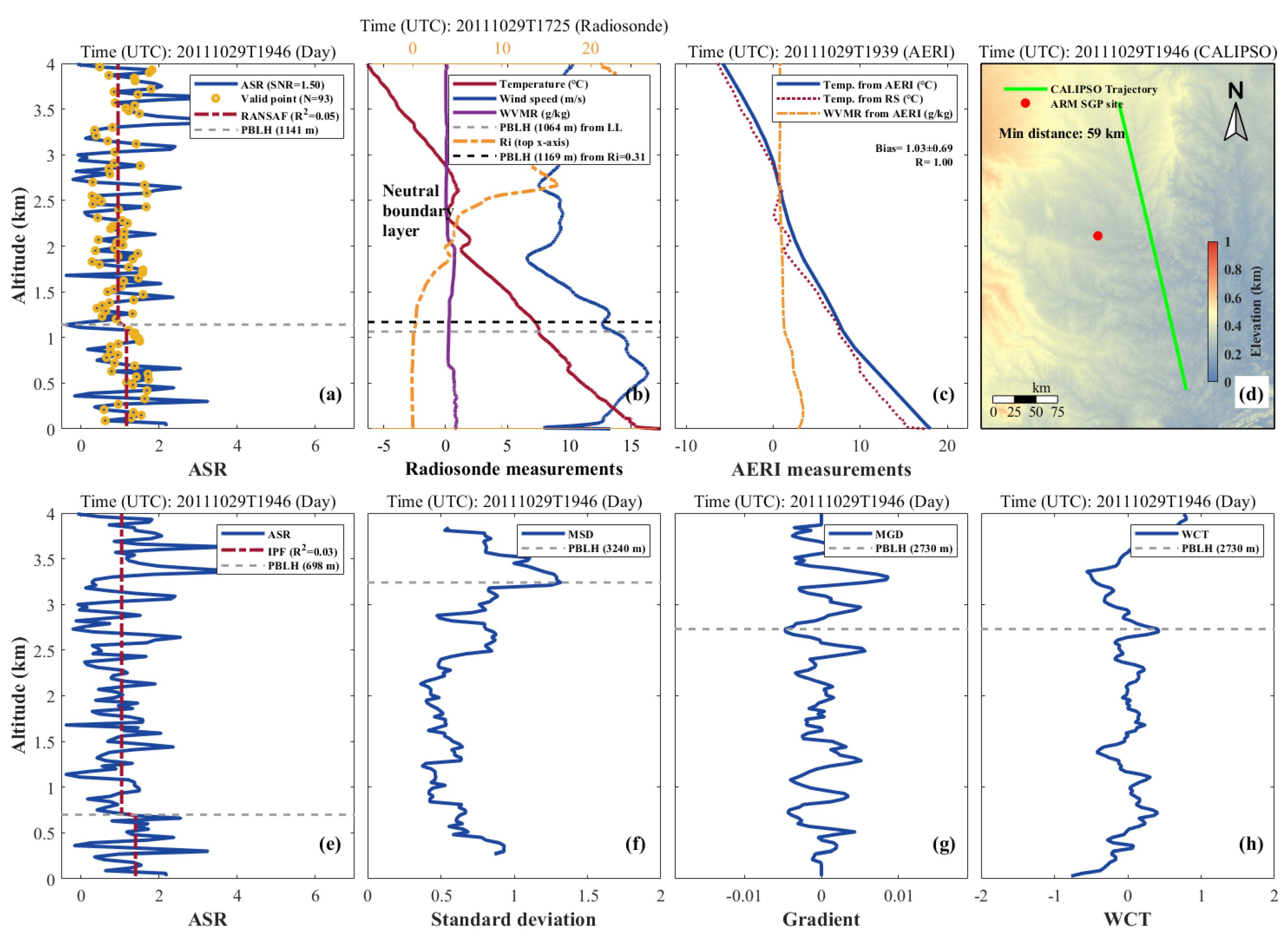
Figure 12 shows a case measured at 19:46:46 UTC (day) on 29 October 2011. The aerosol attenuated layer in ASR profile is from 0 km to 4 km in Figure 12a. The attenuated layers of this ASR profile are indeterminate. The PBLH derived from the RANSAF method displays that the proposed method is ineffective in some measured cases with an indeterminate attenuated layer. Similarly, the traditional methods fail to provide a useful solution in this case. The PBLHs calculated by using the IPF, MSD, MGD, and WCT methods are 698 m, 3240 m, 2730 m, and 2730 m, respectively. These results are different from the result obtained using the radiosonde (1064 m by Liu–Liang method and 1169 m by Ri method). Therefore, this discrepancy remains a difficult problem to solve. Integrating the global wind profile observed by the Aeolus satellite [45] maybe a potential approach to overcome this difficult problem from a single ASR profile from CALIPSO.
6. Conclusions
The effective detection of PBLH from satellite-based lidar signals has been a major challenge for many years. In this study, an improved RANSAF method was proposed on the basis of the integration of random sample consensus theory and the IPF method. The integration can reduce the effects of the cloud layer and significantly fluctuating noise on lidar-based PBLH detection. The RANSAF method includes three steps: single selection, random sample fitting, and self-diagnostics. The performance of the four traditional methods (i.e., MSD, MGD, WCT, and IPF) and the proposed RANSAF method for PBLH determination were compared and analyzed through simulated and measured experiments. In these experiments, the five methods were tested under different conditions, such as presence of strong backscatter layers and low SNR.
The determined PBLHs based on the different methods were validated by radiosonde and AERI measurements. The low PBLH bias derived by the RANSAF method indicates that the improved RANSAF algorithm is a superior method for measuring PBLH under the effects of strong backscatter layers and low SNR in which the traditional methods are mostly ineffective. However, the RANSAF does not work optimally in situations such as multiple attenuated layers and indeterminate attenuated layer.
In this study, only satellite-based signals were tested as examples. Given that this RANSAF algorithm represents practical work, the potential of using the algorithm in further applications of lidar data processing should be examined. Furthermore, integrating the global wind profile observed by the Aeolus satellite maybe a potential approach to improve this study.
Author Contributions
Conceptualization, L.D., Y.P., and W.W.; Methodology, L.D., Y.P., and W.W.; Software, L.D. and Y.P.; Validation, Y.P.; Investigation, L.D.; Writing—original draft preparation, L.D. and Y.P.; Writing—review and editing, W.W.; Visualization, Y.P. and W.W.; Supervision, L.D. and W.W.; Funding acquisition, W.W. All authors have read and agreed to the published version of the manuscript.
Funding
This study was supported by the National Key Research and Development Program of China (grant no. 2018YFC1503600); the National Natural Science Foundation of China (grant no. 41901295); the Natural Science Foundation of Hunan Province, China (grant no. 2020JJ5708); the talents gathering program of Hunan Province, China (grant no. 2018RS3013); the Open Fund of the State Laboratory of Information Engineering in Surveying, Mapping, and Remote Sensing, Wuhan University (Grant No. 18R06); and the leading talents program of Central South University.
Acknowledgments
We are grateful to the Data Center of US NASA (https://search.earthdata.nasa.gov) and data discovery of ARM (https://adc.arm.gov/discovery).
Conflicts of Interest
The authors declare no conflict of interest.
References
- Stull, R.B. An Introduction to Boundary Layer Meteorology; Springer Science and Business Media LLC: Berlin/Heidelberg, Germany, 1988; Volume 13. [Google Scholar]
- Zhang, Y.; Seidel, D.J.; Zhang, S. Trends in Planetary Boundary Layer Height over Europe. J. Clim. 2013, 26, 10071–10076. [Google Scholar] [CrossRef]
- Kong, W.; Yi, F. Convective boundary layer evolution from lidar backscatter and its relationship with surface aerosol concentration at a location of a central China megacity. J. Geophys. Res. Atmos. 2015, 120, 7928–7940. [Google Scholar] [CrossRef]
- Wang, W.; Mao, F.; Zou, B.; Guo, J.; Wu, L.; Pan, Z.; Zang, L. Two-stage model for estimating the spatiotemporal distribution of hourly PM1.0 concentrations over central and east China. Sci. Total Environ. 2019, 675, 658–666. [Google Scholar] [CrossRef] [PubMed]
- Wang, W.; Mao, F.; Du, L.; Pan, Z.; Gong, W.; Fang, S. Deriving Hourly PM2.5 Concentrations from Himawari-8 AODs over Beijing–Tianjin–Hebei in China. Remote Sens. 2017, 9, 858. [Google Scholar] [CrossRef] [Green Version]
- McGrath-Spangler, E.L.; Denning, A.S. Global seasonal variations of midday planetary boundary layer depth from CALIPSO space-borne LIDAR. J. Geophys. Res. Atmos. 2013, 118, 1226–1233. [Google Scholar] [CrossRef]
- Tsaknakis, G.; Papayannis, A.; Kokkalis, P.; Amiridis, V.; Kambezidis, H.D.; Mamouri, R.E.; Georgoussis, G.; Avdikos, G. Inter-comparison of lidar and ceilometer retrievals for aerosol and Planetary Boundary Layer profiling over Athens, Greece. Atmos. Meas. Tech. 2011, 4, 1261–1273. [Google Scholar] [CrossRef] [Green Version]
- Cramer, O.P. Potential Temperature Analysis for Mountainous Terrain. J. Appl. Meteorol. 1972, 11, 44–50. [Google Scholar] [CrossRef]
- Seidel, D.J.; Ao, C.O.; Li, K. Estimating climatological planetary boundary layer heights from radiosonde observations: Comparison of methods and uncertainty analysis. J. Geophys. Res. Space Phys. 2010, 115, 16113. [Google Scholar] [CrossRef] [Green Version]
- Korhonen, K.; Giannakaki, E.; Mielonen, T.; Pfüller, A.; Laakso, L.; Vakkari, V.; Baars, H.; Engelmann, R.; Beukes, J.P.; Van Zyl, P.G.; et al. Atmospheric boundary layer top height in South Africa: Measurements with lidar and radiosonde compared to three atmospheric models. Atmos. Chem. Phys. Discuss. 2014, 14, 4263–4278. [Google Scholar] [CrossRef] [Green Version]
- Zhang, W.; Guo, J.; Miao, Y.; Liu, H.; Zhang, Y.; Li, Z.; Zhai, P. Planetary boundary layer height from CALIOP compared to radiosonde over China. Atmos. Chem. Phys. Discuss. 2016, 16, 9951–9963. [Google Scholar] [CrossRef] [Green Version]
- Hocke, K.; Kämpfer, N.; Gerber, C.; Mätzler, C. A complete long-term series of integrated water vapour from ground-based microwave radiometers. Int. J. Remote Sens. 2011, 32, 751–765. [Google Scholar] [CrossRef]
- Wang, Z.; Cao, X.; Zhang, L.; Notholt, J.; Zhou, B.; Liu, R.; Zhang, B. Lidar measurement of planetary boundary layer height and comparison with microwave profiling radiometer observation. Atmos. Meas. Tech. 2012, 5, 1965–1972. [Google Scholar] [CrossRef] [Green Version]
- Coen, M.C.; Praz, C.; Haefele, A.; Ruffieux, D.; Kaufmann, P.; Calpini, B. Determination and climatology of the planetary boundary layer height above the Swiss plateau by in situ and remote sensing measurements as well as by the COSMO-2 model. Atmos. Chem. Phys. Discuss. 2014, 14, 13205–13221. [Google Scholar] [CrossRef] [Green Version]
- Winker, D.; Hunt, W.H.; McGill, M.J. Initial performance assessment of CALIOP. Geophys. Res. Lett. 2007, 34, L19803. [Google Scholar] [CrossRef] [Green Version]
- Liu, B.; Ma, Y.; Liu, J.; Gong, W.; Wang, W.; Zhang, M. Graphics algorithm for deriving atmospheric boundary layer heights from CALIPSO data. Atmos. Meas. Tech. 2018, 11, 5075–5085. [Google Scholar] [CrossRef] [Green Version]
- Kim, S.-W.; Berthier, S.; Raut, J.-C.; Chazette, P.; Dulac, F.; Yoon, S.-C. Validation of aerosol and cloud layer structures from the space-borne lidar CALIOP using a ground-based lidar in Seoul, Korea. Atmos. Chem. Phys. Discuss. 2008, 8, 3705–3720. [Google Scholar] [CrossRef] [Green Version]
- Liu, J.; Huang, J.; Chen, B.; Zhou, T.; Yan, H.; Jin, H.; Huang, Z.; Zhang, B. Comparisons of PBL heights derived from CALIPSO and ECMWF reanalysis data over China. J. Quant. Spectrosc. Radiat. Transf. 2015, 153, 102–112. [Google Scholar] [CrossRef]
- Su, T.; Li, J.; Li, C.; Xiang, P.; Lau, A.K.-H.; Guo, J.; Yang, D.; Miao, Y. An intercomparison of long-term planetary boundary layer heights retrieved from CALIPSO, ground-based lidar, and radiosonde measurements over Hong Kong. J. Geophys. Res. Atmos. 2017, 122, 3929–3943. [Google Scholar] [CrossRef]
- Leventidou, E.; Zanis, P.; Balis, D.; Giannakaki, E.; Pytharoulis, I.; Amiridis, V. Factors affecting the comparisons of planetary boundary layer height retrievals from CALIPSO, ECMWF and radiosondes over Thessaloniki, Greece. Atmos. Environ. 2013, 74, 360–366. [Google Scholar] [CrossRef]
- Steyn, D.G.; Baldi, M.; Hoff, R.M. The Detection of Mixed Layer Depth and Entrainment Zone Thickness from Lidar Backscatter Profiles. J. Atmos. Ocean. Technol. 1999, 16, 953–959. [Google Scholar] [CrossRef]
- Baars, H.; Ansmann, A.; Engelmann, R.; Althausen, D. Continuous monitoring of the boundary-layer top with lidar. Atmos. Chem. Phys. Discuss. 2008, 8, 7281–7296. [Google Scholar] [CrossRef] [Green Version]
- Eresmaa, N.; Karppinen, A.; Joffre, S.M.; Räsänen, J.; Talvitie, H. Mixing height determination by ceilometer. Atmos. Chem. Phys. Discuss. 2006, 6, 1485–1493. [Google Scholar] [CrossRef] [Green Version]
- Luo, T.; Yuan, R.; Wang, Z. Lidar-based remote sensing of atmospheric boundary layer height over land and ocean. Atmos. Meas. Tech. 2014, 7, 173–182. [Google Scholar] [CrossRef] [Green Version]
- Hayden, K.L.; Anlauf, K.G.; Hoff, R.M.; Strapp, J.W.; Bottenheim, J.W.; Wiebe, H.A.; Froude, F.A.; Martin, J.B.; Steyn, D.G.; McKendry, I.G. The vertical chemical and meteorological structure of the boundary layer in the Lower Fraser Valley during Pacific ’93. Atmos. Environ. 1997, 31, 2089–2105. [Google Scholar] [CrossRef]
- Perrone, M.; Romano, S. Relationship between the planetary boundary layer height and the particle scattering coefficient at the surface. Atmos. Res. 2018, 213, 57–69. [Google Scholar] [CrossRef]
- Mao, F.; Gong, W.; Shalei, S.; Zhu, Z. Determination of the boundary layer top from lidar backscatter profiles using a Haar wavelet method over Wuhan, China. Opt. Laser Technol. 2013, 49, 343–349. [Google Scholar] [CrossRef]
- Brooks, I.M. Finding Boundary Layer Top: Application of a Wavelet Covariance Transform to Lidar Backscatter Profiles. J. Atmos. Ocean. Technol. 2003, 20, 1092–1105. [Google Scholar] [CrossRef] [Green Version]
- Hicks, M.; Sakai, R.; Joseph, E. The Evaluation of a New Method to Detect Mixing Layer Heights Using Lidar Observations. J. Atmos. Ocean. Technol. 2015, 32, 2041–2051. [Google Scholar] [CrossRef]
- Cohn, S.A.; Angevine, W.M. Boundary Layer Height and Entrainment Zone Thickness Measured by Lidars and Wind-Profiling Radars. J. Appl. Meteorol. 2000, 39, 1233–1247. [Google Scholar] [CrossRef]
- Thorsen, T.J.; Fu, Q.; Newsom, R.K.; Turner, D.D.; Comstock, J.M. Automated Retrieval of Cloud and Aerosol Properties from the ARM Raman Lidar. Part I: Feature Detection. J. Atmos. Ocean. Technol. 2015, 32, 1977–1998. [Google Scholar] [CrossRef]
- Atmospheric Radiation Measurement (ARM) User Facility. Updated Hourly. Balloon-Borne Sounding System (SONDEWNPN). 2007-01-01 to 2019-12-31, Southern Great Plains (SGP) Central Facility, Lamont, OK (C1); Holdridge, D., Ritsche, M., Coulter, R., Kyrouac, J., Keeler, E., Eds.; ARM Data Center: Washington, DC, USA, 2020. [CrossRef]
- Liu, S.; Liang, X.-Z. Observed Diurnal Cycle Climatology of Planetary Boundary Layer Height. J. Clim. 2010, 23, 5790–5809. [Google Scholar] [CrossRef]
- Su, T.; Li, Z.; Kahn, R. A new method to retrieve the diurnal variability of planetary boundary layer height from lidar under different thermodynamic stability conditions. Remote Sens. Environ. 2020, 237, 111519. [Google Scholar] [CrossRef]
- Zhang, Y.; Gao, Z.; Li, D.; Li, Y.; Zhang, N.; Zhao, X.; Chen, J. On the computation of planetary boundary-layer height using the bulk Richardson number method. Geosci. Model Dev. 2014, 7, 2599–2611. [Google Scholar] [CrossRef] [Green Version]
- Feltz, W.F.; Smith, W.L.; Howell, H.B.; Knuteson, R.; Woolf, H.; Revercomb, H.E. Near-Continuous Profiling of Temperature, Moisture, and Atmospheric Stability Using the Atmospheric Emitted Radiance Interferometer (AERI). J. Appl. Meteorol. 2003, 42, 584–597. [Google Scholar] [CrossRef]
- Winker, D.; Vaughan, M.A.; Omar, A.; Hu, Y.; Powell, K.A.; Liu, Z.; Hunt, W.H.; Young, S.A. Overview of the CALIPSO Mission and CALIOP Data Processing Algorithms. J. Atmos. Ocean. Technol. 2009, 26, 2310–2323. [Google Scholar] [CrossRef]
- Liu, Z.; Vaughan, M.A.; Winker, D.; Kittaka, C.; Getzewich, B.; Kuehn, R.; Omar, A.; Powell, K.; Trepte, C.; Hostetler, C. The CALIPSO Lidar Cloud and Aerosol Discrimination: Version 2 Algorithm and Initial Assessment of Performance. J. Atmos. Ocean. Technol. 2009, 26, 1198–1213. [Google Scholar] [CrossRef]
- Vaughan, M.; Winker, D.M.; Powell, K. CALIOP Algorithm Theoretical Basis Document, Part 2: FEATURE Detection and Layer Properties Algorithms; NASA Langley Research Center: Hampton, VA, USA, 2005.
- Earth Resources Observation and Science (EROS) Center. GTOPO30 Documentation (README File). USGS: Reston, VA, USA, 1997. Available online: https://www.usgs.gov/science-explorer-results?es=GTOPO30+ (accessed on 19 March 2020).
- NOAA; NASA; USAF. US Standard Atmosphere, 1976; National Oceanic and Atmospheric Administration: Washington, DC, USA, 1976; Volume 76.
- Fischler, M.A.; Bolles, R.C. Random sample consensus: A paradigm for model fitting with applications to image analysis and automated cartography. Commun. ACM 1981, 24, 381–395. [Google Scholar] [CrossRef]
- Compton, J.C.; Delgado, R.; Berkoff, T.A.; Hoff, R.M. Determination of Planetary Boundary Layer Height on Short Spatial and Temporal Scales: A Demonstration of the Covariance Wavelet Transform in Ground-Based Wind Profiler and Lidar Measurements. J. Atmos. Ocean. Technol. 2013, 30, 1566–1575. [Google Scholar] [CrossRef]
- Ma, X.; Wang, C.; Han, G.; Ma, Y.; Li, S.; Gong, W.; Chen, J. Regional Atmospheric Aerosol Pollution Detection Based on LiDAR Remote Sensing. Remote Sens. 2019, 11, 2339. [Google Scholar] [CrossRef] [Green Version]
- Guo, J.; Liu, B.; Gong, W.; Shi, L.; Zhang, Y.; Ma, Y.; Zhang, J.; Chen, T.; Bai, K.; Stoffelen, A.; et al. Technical Note: First comparison of wind observations from ESA’s satellite mission Aeolus and ground-based Radar wind profiler network of China. Atmos. Chem. Phys. Discuss. 2020, 2020, 1–36. [Google Scholar] [CrossRef]
Figure 1.
Location of the Southern Great Plains (SGP) central facility site. The white and black lines refer to the CALIPSO trajectory in the daytime and nighttime, respectively.
Figure 1.
Location of the Southern Great Plains (SGP) central facility site. The white and black lines refer to the CALIPSO trajectory in the daytime and nighttime, respectively.

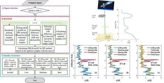
Figure 2.
Flowchart of RANSAF method to determine the PBLH from the satellite-based lidar signal.

Figure 3.
PBLHs determined with (a) IPF, (c) RANSAF, (d) MSD, (e) MGD, and (f) WCT methods from a simulated ASR. (b) Ideal profile fitted by the randomly selected points.
Figure 3.
PBLHs determined with (a) IPF, (c) RANSAF, (d) MSD, (e) MGD, and (f) WCT methods from a simulated ASR. (b) Ideal profile fitted by the randomly selected points.

Figure 4.
Diagram of ASR derived from CALIOP.

Figure 5.
ASR was measured by CALIOP at 08:38:40 UTC (night) on 26 May 2015; PBLHs were determined with the (a) RANSAF, (b) radiosonde (RS), (e) IPF, (f) MSD, (g) MGD, and (h) WCT methods; (c) vertical profile of temperature and water vapor mixing ratio (WVMR) retrieved from AERI with the red dotted line referring to temperature measured by RS in (b), Bias (R) is the mean difference (correlation coefficient) between temperature profiles from AERI and RS; (d) ARM SGP site of radiosonde observations and CALIPSO trajectory. The minimum distance between the CALIOP and radiosonde (AERI) measurements are shown at the top of subfigure (d).

Figure 6.
ASR was measured by CALIOP at 19:47:51 UTC (day) on 24 March 2013; PBLHs were determined with the (a) RANSAF, (b) radiosonde (RS), (e) IPF, (f) MSD, (g) MGD, and (h) WCT methods; (c) vertical profile of temperature and water vapor mixing ratio (WVMR) retrieved from AERI with the red dotted line referring to temperature measured by RS in (b), Bias (R) is the mean difference (correlation coefficient) between temperature profiles from AERI and RS; (d) ARM SGP site of radiosonde observations and CALIPSO trajectory. The minimum distance between the CALIOP and radiosonde (AERI) measurements are shown in the top of subfigure (d).

Figure 7.
ASR was measured by CALIOP from 19:49:29 to 19:50:19 on 23 October 2009 (UTC, daytime); PBLHs were determined with (a) MSD, (b) MGD, (c) WCT, (d) IPF, and (e) RANSAF methods.
Figure 7.
ASR was measured by CALIOP from 19:49:29 to 19:50:19 on 23 October 2009 (UTC, daytime); PBLHs were determined with (a) MSD, (b) MGD, (c) WCT, (d) IPF, and (e) RANSAF methods.

Figure 8.
PBLHs were determined with the (a) radiosonde (RS) at 17:28 and (b) AERI at 19:43 on 21 October 2009 (UTC); (c) ARM SGP site of radiosonde observations and CALIPSO trajectory. The minimum distance between the CALIOP and radiosonde (AERI) measurements are shown in the top of subfigure (c).
Figure 8.
PBLHs were determined with the (a) radiosonde (RS) at 17:28 and (b) AERI at 19:43 on 21 October 2009 (UTC); (c) ARM SGP site of radiosonde observations and CALIPSO trajectory. The minimum distance between the CALIOP and radiosonde (AERI) measurements are shown in the top of subfigure (c).

Figure 9.
ASR measured using CALIOP from 08:40:03 to 08:40:53 on 19 December 2009 (UTC, nighttime); PBLHs were determined by using (a) MSD, (b) MGD, (c) WCT, (d) IPF, and (e) RANSAF methods.
Figure 9.
ASR measured using CALIOP from 08:40:03 to 08:40:53 on 19 December 2009 (UTC, nighttime); PBLHs were determined by using (a) MSD, (b) MGD, (c) WCT, (d) IPF, and (e) RANSAF methods.

Figure 10.
PBLHs were determined using the (a) radiosonde (RS) at 11:24 and (b) AERI at 08:36 on 19 December 2009 (UTC, nighttime); (c) ARM SGP site of radiosonde observations and CALIPSO trajectory. The minimum distance between the CALIOP and radiosonde (AERI) measurements is shown at the top of subfigure (c).

Figure 11.
ASR was measured using CALIOP at 19:46:46 UTC (day) on 31 August 2007; PBLHs were determined by using (a) RANSAF, (b) radiosonde (RS), (e) IPF, (f) MSD, (g) MGD, and (h) WCT methods; (c) vertical profile of temperature and water vapor mixing ratio (WVMR) retrieved from AERI with the red dotted line refer to the temperature measured by RS in (b), Bias (R) is the mean difference (correlation coefficient) between temperature profiles from AERI and RS; (d) ARM SGP site of radiosonde observations and CALIPSO trajectory. The minimum distance between the CALIOP and radiosonde (AERI) measurements are shown at the top of subfigure (d).

Figure 12.
ASR was measured using CALIOP at 19:46:46 UTC (day) on 29 October 2011; PBLHs were determined by using the (a) RANSAF, (b) radiosonde (RS), (e) IPF, (f) MSD, (g) MGD, and (h) WCT methods; (c) vertical profile of temperature and water vapor mixing ratio (WVMR) retrieved from AERI with the red dotted line refer to the temperature measured by RS in (b), Bias (R) is the mean difference (correlation coefficient) between temperature profiles from AERI and RS; (d) ARM SGP site of radiosonde observations and CALIPSO trajectory. The minimum distance between the CALIOP and radiosonde (AERI) measurements are shown at the top of subfigure (d).

Publisher’s Note: MDPI stays neutral with regard to jurisdictional claims in published maps and institutional affiliations. |
© 2020 by the authors. Licensee MDPI, Basel, Switzerland. This article is an open access article distributed under the terms and conditions of the Creative Commons Attribution (CC BY) license (http://creativecommons.org/licenses/by/4.0/).
Share and Cite
MDPI and ACS Style
Du, L.; Pan, Y.; Wang, W. Random Sample Fitting Method to Determine the Planetary Boundary Layer Height Using Satellite-Based Lidar Backscatter Profiles. Remote Sens. 2020, 12, 4006. https://0-doi-org.brum.beds.ac.uk/10.3390/rs12234006
AMA Style
Du L, Pan Y, Wang W. Random Sample Fitting Method to Determine the Planetary Boundary Layer Height Using Satellite-Based Lidar Backscatter Profiles. Remote Sensing. 2020; 12(23):4006. https://0-doi-org.brum.beds.ac.uk/10.3390/rs12234006
Chicago/Turabian StyleDu, Lin, Ya’ni Pan, and Wei Wang. 2020. "Random Sample Fitting Method to Determine the Planetary Boundary Layer Height Using Satellite-Based Lidar Backscatter Profiles" Remote Sensing 12, no. 23: 4006. https://0-doi-org.brum.beds.ac.uk/10.3390/rs12234006
Note that from the first issue of 2016, this journal uses article numbers instead of page numbers. See further details here.