Lookup Table Approach for Radiometric Calibration of Miniaturized Multispectral Camera Mounted on an Unmanned Aerial Vehicle

Abstract

Over recent years, miniaturized multispectral cameras mounted on an unmanned aerial vehicle (UAV) have been widely used in remote sensing. Most of these cameras are integrated with low-cost, image-frame complementary metal-oxide semiconductor (CMOS) sensors. Compared to the typical charged coupled device (CCD) sensors or linear array sensors, consumer-grade CMOS sensors have the disadvantages of low responsivity, higher noise, and non-uniformity of pixels, which make it difficult to accurately detect optical radiation. Therefore, comprehensive radiometric calibration is crucial for quantitative remote sensing and comparison of temporal data using such sensors. In this study, we examine three procedures of radiometric calibration: relative radiometric calibration, normalization, and absolute radiometric calibration. The complex features of dark current noise, vignetting effect, and non-uniformity of detector response are analyzed. Further, appropriate procedures are used to derive the lookup table (LUT) of correction factors for these features. Subsequently, an absolute calibration coefficient based on an empirical model is used to convert the digital number (DN) of images to radiance unit. Due to the radiometric calibration, the DNs of targets observed in the image are more consistent than before calibration. Compared to the method provided by the manufacturer of the sensor, LUTs facilitate much better radiometric calibration. The root mean square error (RMSE) of measured reflectance in each band (475, 560, 668, 717, and 840 nm) are 2.30%, 2.87%, 3.66%, 3.98%, and 4.70% respectively.

1. Introduction

Over recent years, miniaturized multispectral cameras based on cost-effective sensors have been extensively applied in the remote sensing field [1,2,3,4,5,6], such as MicaSense RedEdge-MX (MicaSense Inc., Seattle, WA, USA), MS600 pro (Changguang YuSense Information Technology and Equipment (Qingdao) Co., Ltd., Qingdao, China), and Parrot Sequoia (Parrot Drone SAS, Paris, France). Such multispectral cameras are usually mounted on unmanned aerial vehicles (UAVs), which facilitates individual researchers, small teams, or commercial industries to obtain spectral information with ultra-high spatial resolution [7]. From the perspective of a low-cost and lightweight device, consumer-grade complementary metal-oxide semiconductor (CMOS) sensors are the main choice for integrating such multispectral cameras. In contrast to the typical remote sensing sensors that are mostly based on a linear charged coupled device (CCD) or scientific-grade CCD, the two-dimensional (2D) frame, low-cost CMOS sensors pose several challenges in the remote sensing applications: (1) CMOS detectors tend to generate more noise as each photodiode of a CMOS sensor needs an amplifier. (2) Because the sensitive area of each pixel is much smaller than its surface area, the sensitivity of the CMOS sensor is lower than that of a CCD sensor. (3) Besides, the 2D-frame structure is more complex than the linear structure in terms of the vignetting effect of lens and response of detectors [8,9,10,11]. Therefore, accurate radiometric calibration is the key to the effective application of multispectral cameras based on consumer-grade CMOS sensors in quantitative remote sensing.

The electro-optical performance of sensors is mainly affected by three intrinsic elements: dark current, vignetting effect, and detector response [12,13,14]. These are apparently non-uniform in each pixel and have the characteristics of spatial configurations within the images [1,14,15]. These phenomena are more serious in CMOS sensors [8,13,16,17,18]. The dark current is related to the sensor’s temperature, gain, and integration time, and it is corrected by estimating the non-uniformity of the dark signal [7,9,19]. The non-uniformity of the dark current is usually eliminated through image templates obtained by blocking the lens under normal working conditions [20,21,22]. Vignetting correction is a challenging process, and it is usually performed by two methods: the lookup table (LUT) method [23,24] and the polynomial fitting method [25]. The LUT method is considered to be the most accurate method for vignetting correction [26,27]. The response factor may vary randomly among detectors due to the inherent cell-to-cell variations introduced during the manufacturing process. D. Olsen et al. [14] determined correction coefficients to minimize the effects of optical vignetting, non-uniform quantum efficiency of a CCD, and dark current of a CCD using a least-squares fit approach. Moreover, when the radiation intensity is converted to a digital number (DN), the quantized value varies with the tunable parameters of sensors such as integration time and gain. Therefore, the DN needs to be normalized with different camera settings [1,19,28]. The parameters of absolute radiometric calibration including correction coefficients and offset are typically derived using a linear model [4,18,29]. However, a clear understanding of the representativeness of image templates for non-uniform dark current and the relationship between dark current and sensor characteristics (e.g., integration time and gain) is lacking in the existing literature. Moreover, vignetting correction has been primarily based on the mathematical model of the polynomial fitting, and the LUT method with higher precision has been rarely used for this correction.

This study primarily focuses on determining the parameter LUTs for radiometric calibration and verify their accuracy for a miniaturized multispectral camera integrated with 2D-frame CMOS sensors. The image templates corresponding to the non-uniformity of dark current, LUT of vignetting correction, and response factor of each cell are all considered to obtain the correction factor LUTs. This is achieved by dividing the radiometric calibration model into three steps: relative radiometric calibration, normalization, and absolute radiometric calibration. Due to the complex radiation characteristics of the sensors, the determination of LUTs of optimal calibration factors corresponding to relative radiometric calibration is the most critical and challenging process, particularly for vignetting correction [26,30]. The main ideas of this study are based on the methods proposed by D. Olsen et al. [14]. We extend their idea to the 2D-frame sensors by selecting different solutions for attaining the 2D-frame LUTs to calibrate the dark current, vignetting effect, and detection response. Solutions are selected based on the image characteristics to improve the performance of calibration.

The rest of this paper is organized as follows. The procedures for obtaining the LUTs of calibration factors of dark current, vignetting effect, and detection response are explained in Section 2. The multispectral camera, light source, and experimental method are also described. In Section 3, the dark current, vignetting effect, detection response, and the absolute calibration parameters are experimentally analyzed. Further, a verification method is introduced to validate the accuracy of experimental results. Then, relative and absolute accuracies are examined and compared with the calibration results based on the method provided by the sensor’s manufacturer. The principle, methods, main results, limitations, and future scope of the study are discussed in Section 4. Finally, the study is concluded in Section 5.

2. Materials and Methods

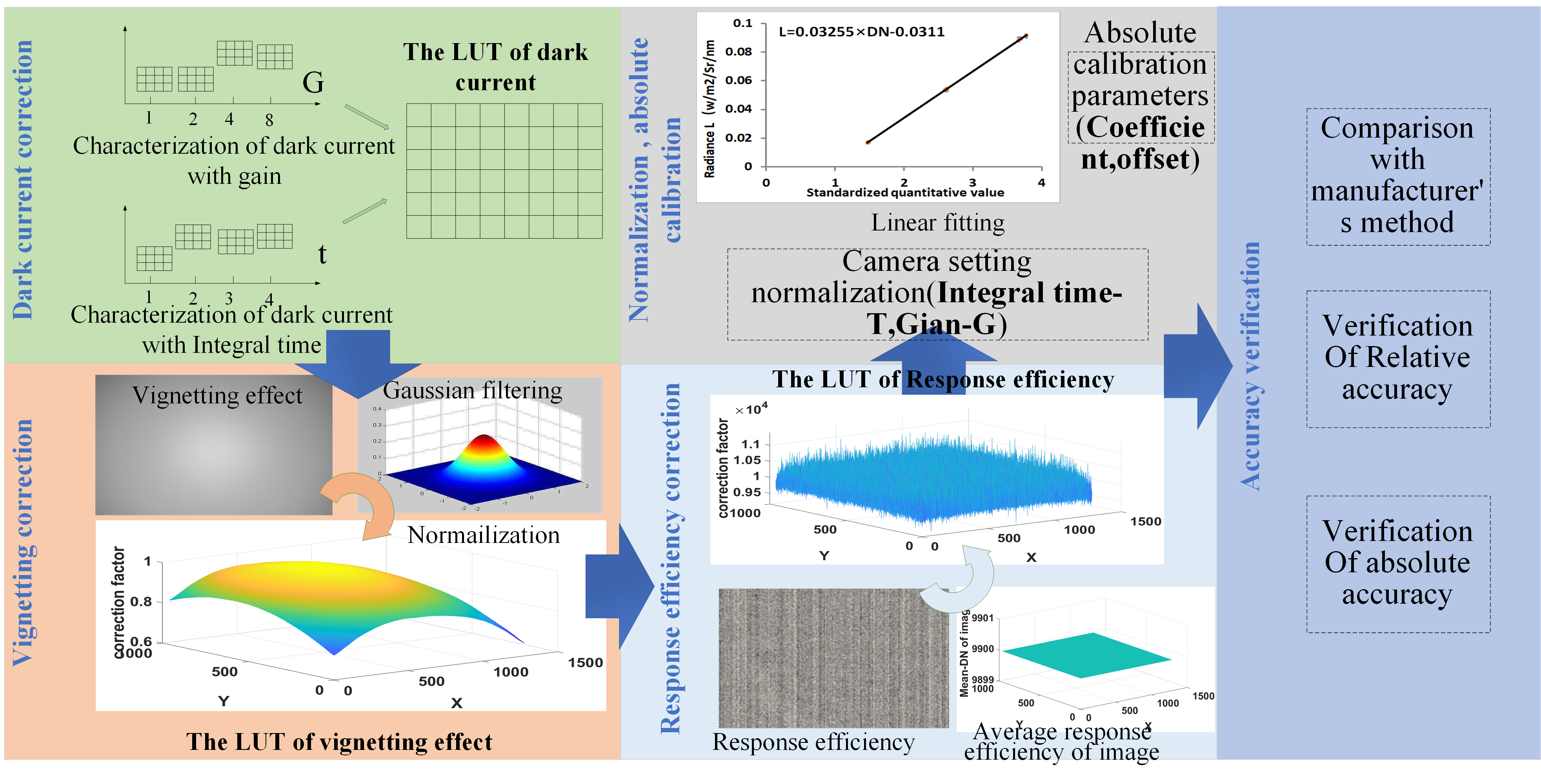
2.1. Multispectral Camera and Experimental System

2.1.1. Calibration of Multispectral Camera

Radiometric calibration was implemented on a miniaturized multispectral camera manufactured by MicaSense, Inc., America. MicaSense RedEdge-MX is an advanced multispectral camera specially designed for small, unmanned aircraft systems. It includes compact bundles (rigs) of five cameras with CMOS sensors. The size of each CMOS sensor is 1280 × 960. This multispectral camera uses narrow-pass filters to control the incident light and can simultaneously capture five discrete spectral bands (blue, green, red, red edge, near-infrared) [17,31,32]. The detailed parameters of the sensor are displayed in

Table 1. Characteristics of sensors and lens.

Parameter	Value	Parameter	Value
Spectral bands (Band1–Band5)	Blue (475 nm), green (560 nm), red (668 nm), red edge (717 nm), and near-infrared (840 nm)	Shutter mode	Global shutter
Image size	4.8 × 3.6 mm2	Field of view (FOV) of less	47.2° HFOV
Imager resolution	1280 × 960 pixels	Focal length of lens	5.4 mm
Average pixel size of image	3.75 μm	Integration time	0.066–24.5 ms
Gain values [32]	1×, 2×, 4×, 8×	RAW Format	12-bit DNG or 16-bit TIFF
Exposure time	0.066–24.5 ms	Ground sample distance	8 cm per pixel (per band) at 120 m (~400 ft) above ground level (AGL)

. The spectral response of the sensor and transmittance of filters for each band are shown in Figure 1 [32].

Typically, MicaSense RedEdge-MX is used to generate precise and quantitative information on the vigor and health of crops. For aviation applications at low altitudes, the integration time should not be too high or too low to avoid insufficient exposure and the affect of image motion on the geometric accuracy. An integration time in the range of 1/2000–1/500 s is an appropriate and common choice [19,22,33].

2.1.2. Integrating Sphere System

The radiation characteristics of the sensor were observed using an integrating sphere (XTH2000, Labsphere Inc., North Sutton, NH, USA). The structure of the integrating sphere system and the measurement scheme are shown in Figure 2. The integrating sphere provided stable and uniform optical radiation in the wavelength range of 300–2400 nm. Its aperture was 20 cm, and the optical uniformity was more than 98%.

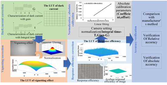
2.2. Derivation of LUTs

2.2.1. Radiometric Calibration Model

The DN recorded by the detectors of CMOS sensors looking at a target with emitting radiance $L\left(x,y\right)$ were modeled as follows [5,12,13,14,34]:

$$L\left(x,y\right)=a\ast \frac{1}{g\ast t_e\ast 2^N}\ast \frac{1}{R\left(x,y\right)}\ast \frac{1}{V\left(x,y\right)}\ast \left[D{N}_s\left(x,y\right)-\mathrm{Dark}\left(x,y\right)\right]+b$$

(1)

where $x,y$ was the position of the target on the image; $R\left(x,y\right)$ was the correction factor at $x,y$ in the LUT of response; $V\left(x,y\right)$ was the correction factor at $x,y$ in the LUT of vignetting effect; $\mathrm{Dark}\left(x,y\right)$ was the correction factor at $x,y$ in the LUT of dark current; $DN\left(x,y\right)$ was the raw pixel value at $x,y$; $g$ and $t_e$ were the gain and integration time of sensors, respectively; $2^N$ was the digital bit rate (8 bit, 12 bit, 16 bit); N was the number of bits; $a\mathrm{and}b$ were the quantization parameters of analog-to-digital conversion, namely quantized coefficient and offset of absolute radiometric calibration, respectively.

The radiometric calibration process was divided into three steps: relative radiometric calibration, data normalization, and absolute radiometric calibration. Equation (1) could be simplified by decomposing it into three parts.

Firstly, relative radiometric calibration made DN values comparable within the image. The main task of the relative radiometric calibration was to eliminate the influence of dark current, vignetting effect, and non-uniform detection efficiency [2,13,17,18,35].

$$D{N}_c=\frac{1}{R\left(x,y\right)}\ast \frac{1}{V\left(x,y\right)}\ast \left[D{N}_s\left(x,y\right)-\mathrm{Dark}\left(x,y\right)\right]$$

(2)

Secondly, data normalization made the images, which were captured under different camera parameter settings, comparable [3,14,33].

$$D{N}_n=\frac{1}{g}\ast \frac{1}{t_e}\ast \frac{1}{2^N}{\ast \mathrm{DN}}_c$$

(3)

Thirdly, absolute radiometric calibration converted DN into physical units of radiance ($\mathrm{W}·{\mathrm{m}}^{-2}·{\mathrm{Sr}}^{-1}·{\mathrm{nm}}^{-1}$). A linear empirical model is often used for absolute radiometric calibration [4,12,18,36].

$$L_0=a\ast D{N}_n+b$$

(4)

Based on Equations (2)–(4), DN could be converted to the radiance unit only if the LUTs of $\mathrm{Dark}\left(x,y\right)$, $V\left(x,y\right),$ $R\left(x,y\right)$, $a,b$ were derived. In the next step, we adopted reasonable solutions to obtain these parameter LUTs in experiments so that the incident radiation field for an arbitrary operational image could be determined.

2.2.2. Correction of Dark Current

The correction parameters of dark current were defined in terms of the LUT of non-uniformity in 2D image space rather than the mean value of dark current in the image [7,9,17]. To reduce the complexity of the dark current correction, a representative template was selected as the LUT of dark current. This LUT was an effective choice to eliminate dark current for images taken under different camera settings of gain and integration time. The dark current was characterized by gain and integration time to determine the representative template after the temperature of the device was stabilized. The LUT of dark current can be obtained as following procedure in Figure 3.

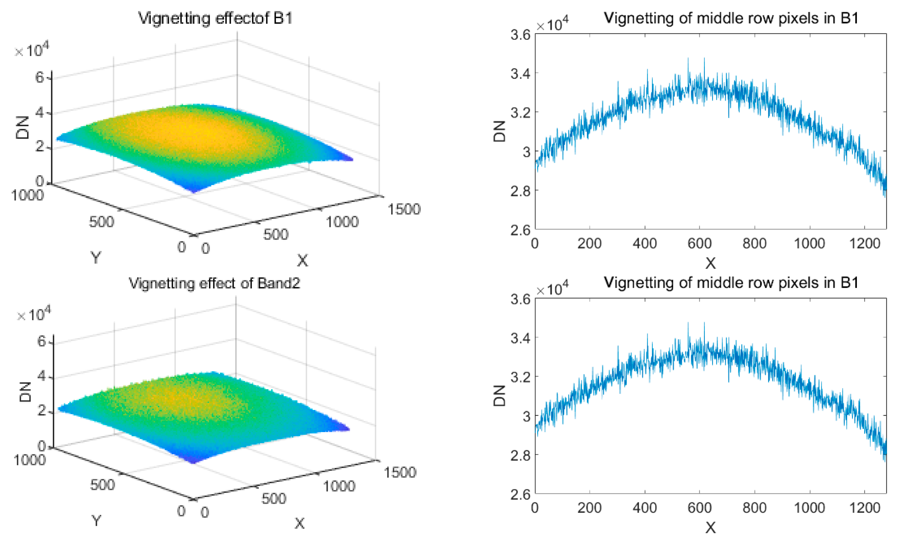
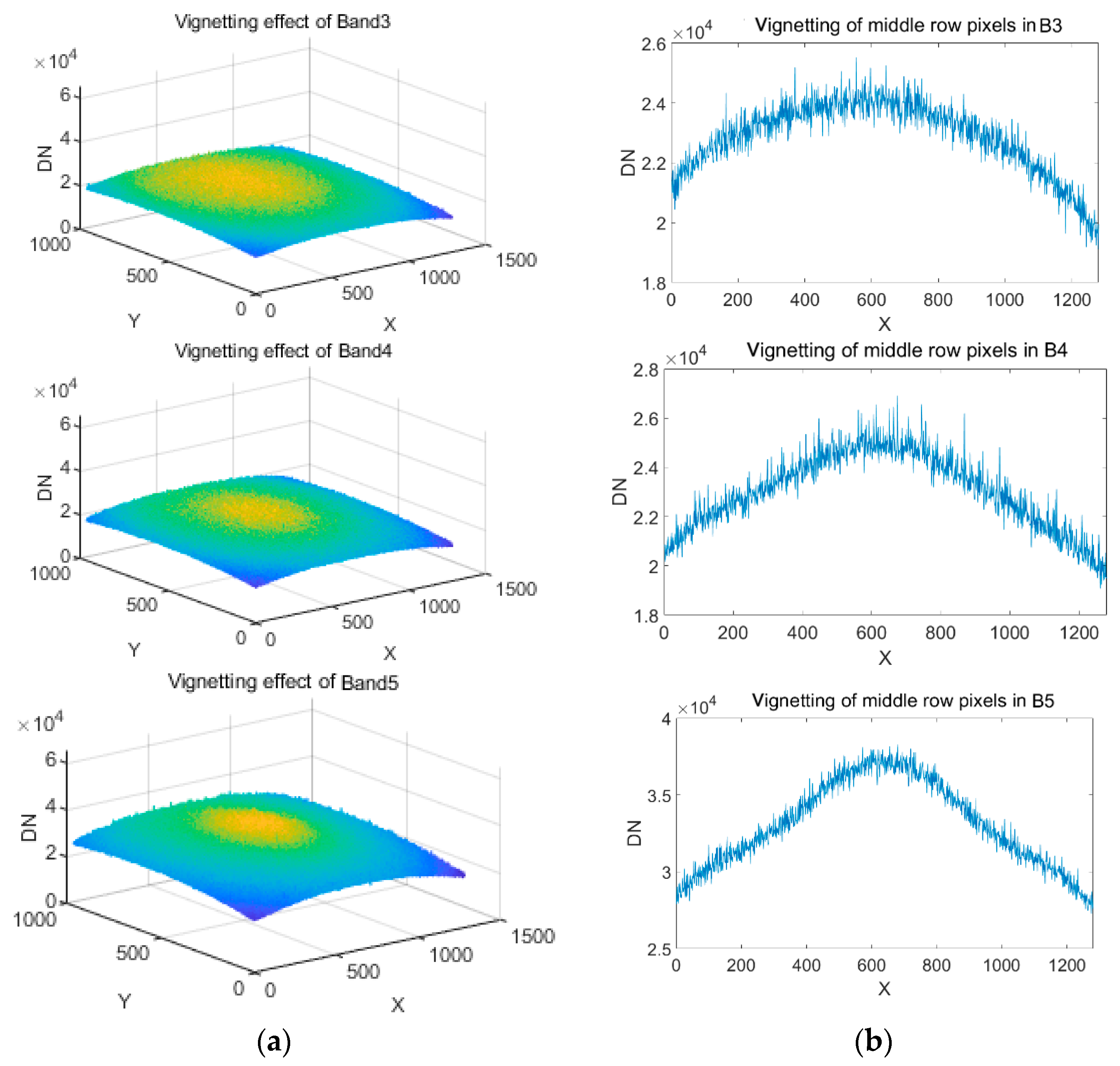
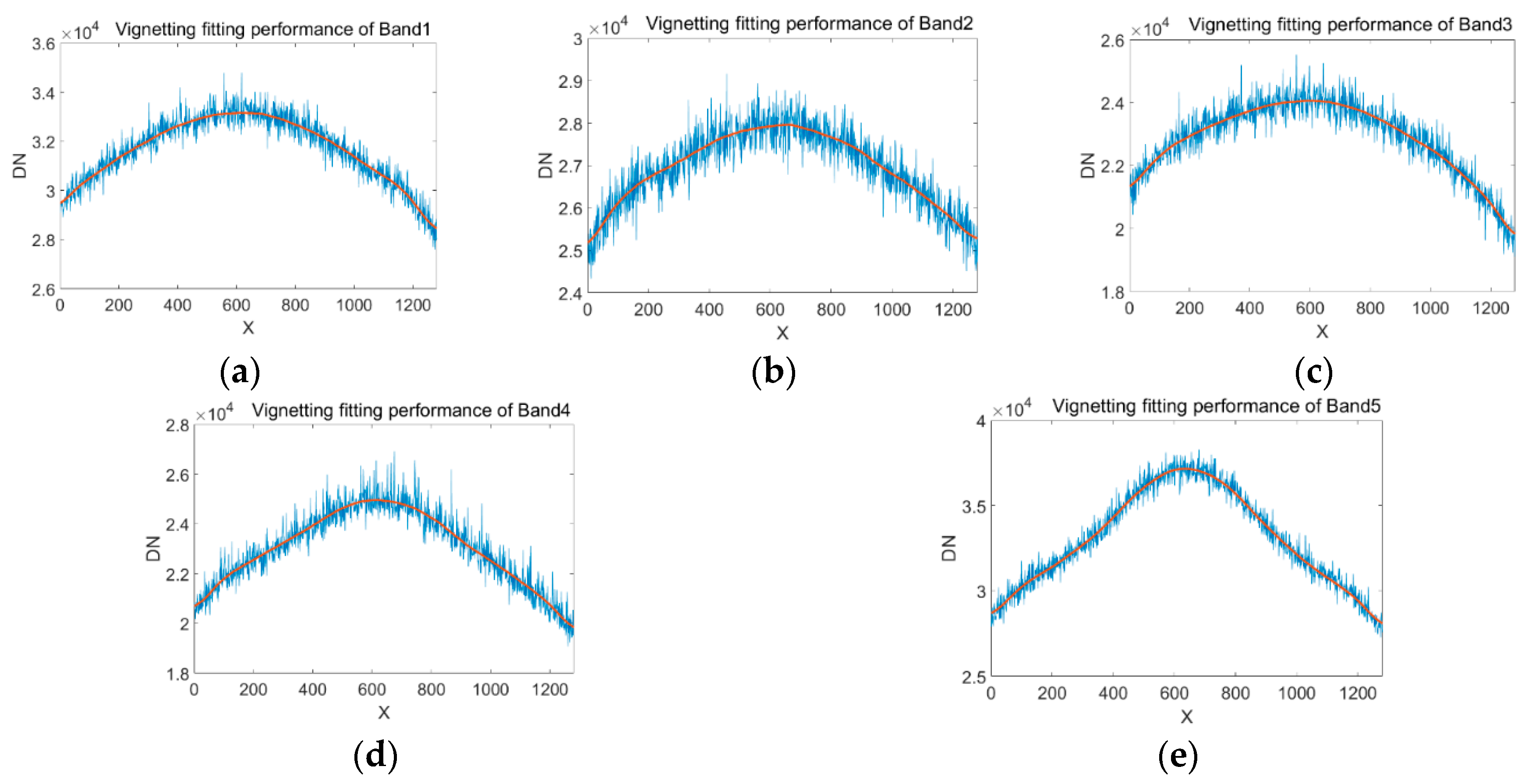
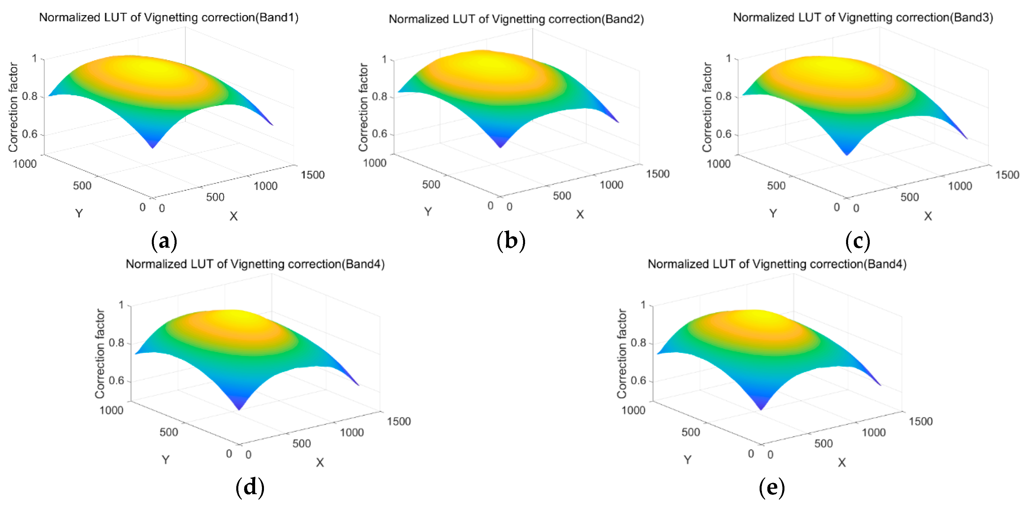
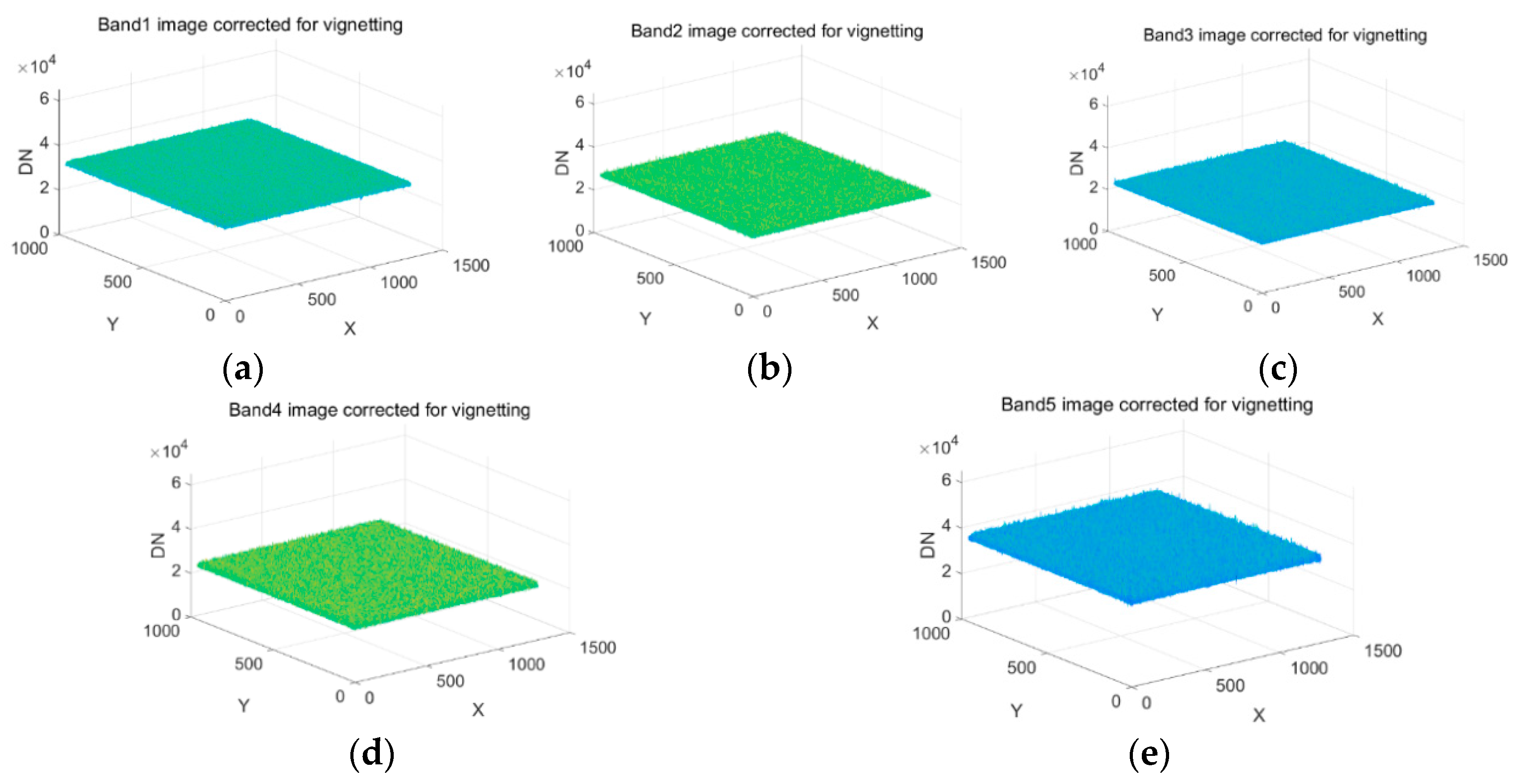
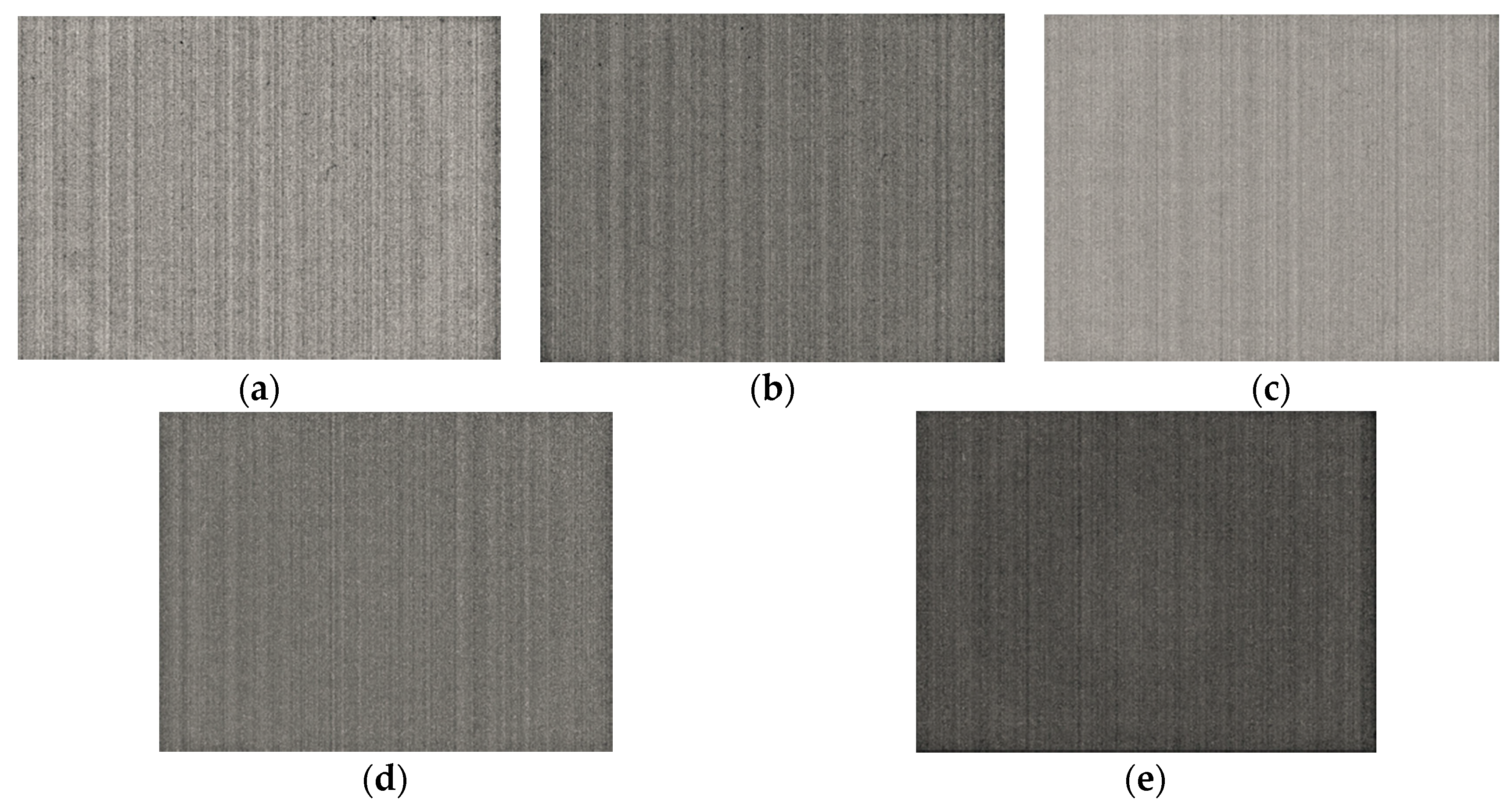
2.2.3. Vignetting Effect Correction

Vignetting is a phenomenon in which the center of the image is brighter and the edge area is darker due to the limitation of apertures and defects of optical devices [26,31,37]. Polynomial fitting based on radial distance is commonly utilized for vignetting correction of miniaturized multispectral cameras [25,38,39]. Due to the imperfect manufacturing process, the brightness center is not consistent with the sensor center and is difficult to determine. The vignetting effect on 2D images is more complex and may be asymmetric. In practice, there can be deviations in the polynomial fitting. The vignetting correction method based on image LUT has high correction accuracy [17,25,29]. Each pixel has a unique correction factor in the LUT of vignetting correction.

Theoretically, a vignette is a gentle gradient from the middle to the edge [40]. Due to the non-uniform response and the influence of random noise, the images of uniform objects are not smooth. Thus, in an image obtained with uniform incident light, the vignetting effect corresponds to low frequency, while random noise and response noise are high-frequency noises. Here, the Gaussian low-pass filtering method was selected to eliminate random noise and response noise and extract background brightness from the vignetting images. The filter could prevent distortion of the edge signal in the smoothing process [15,25].

$$filte{r}_{gaussian}\left(x,y\right)=\frac{1}{2\pi {\sigma }^2}{e}^{-\frac{x^2+y^2}{2{\sigma }^2}}$$

(5)

$$V=image\ast filte{r}_{gaussian}$$

(6)

Then, the vignetting image was normalized through the correction factors. $v\left(x,y\right)$ was the pixel value in the vignetting image;$V_{max}$. was the maximum pixel value within the vignetting image.

$$Normaliz\_V\left(x,y\right)=\frac{V\left(x,y\right)}{V_{max}}$$

(7)

Several normalized vignetting images were obtained at different incident radiation levels. The effective LUT of the vignetting correction represented the mean image of several normalized vignetting images.

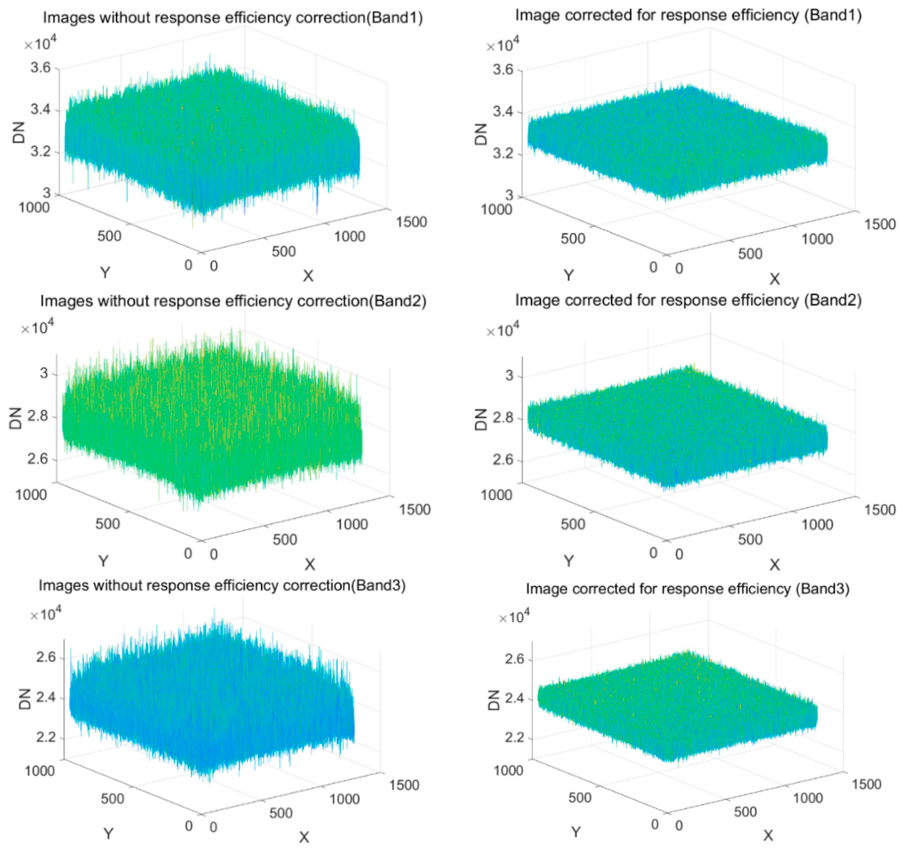
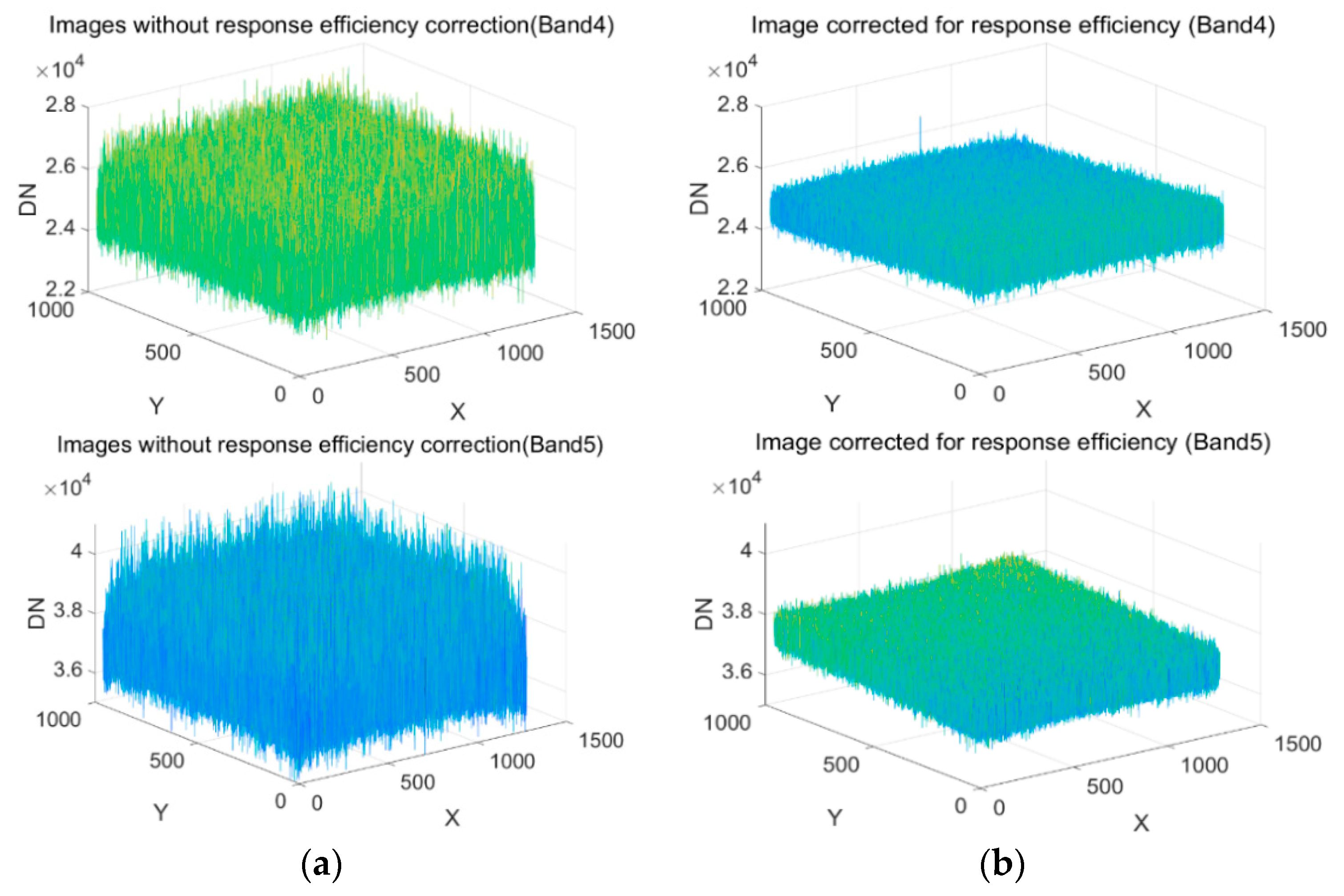
2.2.4. Response Correction

After correction of dark current and vignetting effect, images captured under a uniform illumination retained the error of non-uniform pixel response and random noise. Under standard and uniform illumination, the photoelectric response of each detector in CMOS was inconsistent due to the imperfect manufacturing process [6,34]. Here, multiple images under the same radiance of the integrating sphere were corrected for dark current and vignetting effect. Then, these corrected images were averaged to eliminate random noise.

The correction factor of the response function was defined as the ratio of pixel response value to the average response value. The pixel response value and average response value were obtained after correcting the image for dark current and vignetting effect.

$$R\left(x,y\right)=\frac{image\left(x,y\right)}{{Mean}_{image}}$$

(8)

Similarly, the effective LUT of response correction represented the mean image of several corrected images obtained at different incident radiation levels.

2.2.5. Parameters of Absolute Radiometric Calibration

According to Equations (3) and (4), the linear fitting method was used to derive the coefficient and offset. The dataset used for linear fitting was collected at the different radiation intensities and camera settings of gain and integration time. This dataset must be corrected using relative radiometric calibration beforehand. Linear fitting indicated a linear causal relationship between two variables, i.e.,

$$Y_i=a{X}_i+b+{\epsilon }_i\left(i=1,2,3\cdots n\right)$$

(9)

where $i$ was the number of observed value; $a\mathrm{and}b$ were the fitting coefficient and offset, respectively; $a{X}_i+b$ expressed the linear relationship between $Y\mathrm{and}X$. ${\epsilon }_i$ was a random variable that reflected the distribution around the straight line of statistical relationship and obeyed normal distribution.$a\mathrm{and}b$ were statistically analyzed based on the sample dataset. The evaluated values of a and b were $\alpha \mathrm{and}\beta$, which obeyed the following linear equation:

$$\widehat{Y}=\alpha X+\beta$$

(10)

Generally, $\alpha$ and $\beta$ should be calculated to minimize the deviation between each sample observation point $\left(Y_i,X_i\right)$ and the fitting line.

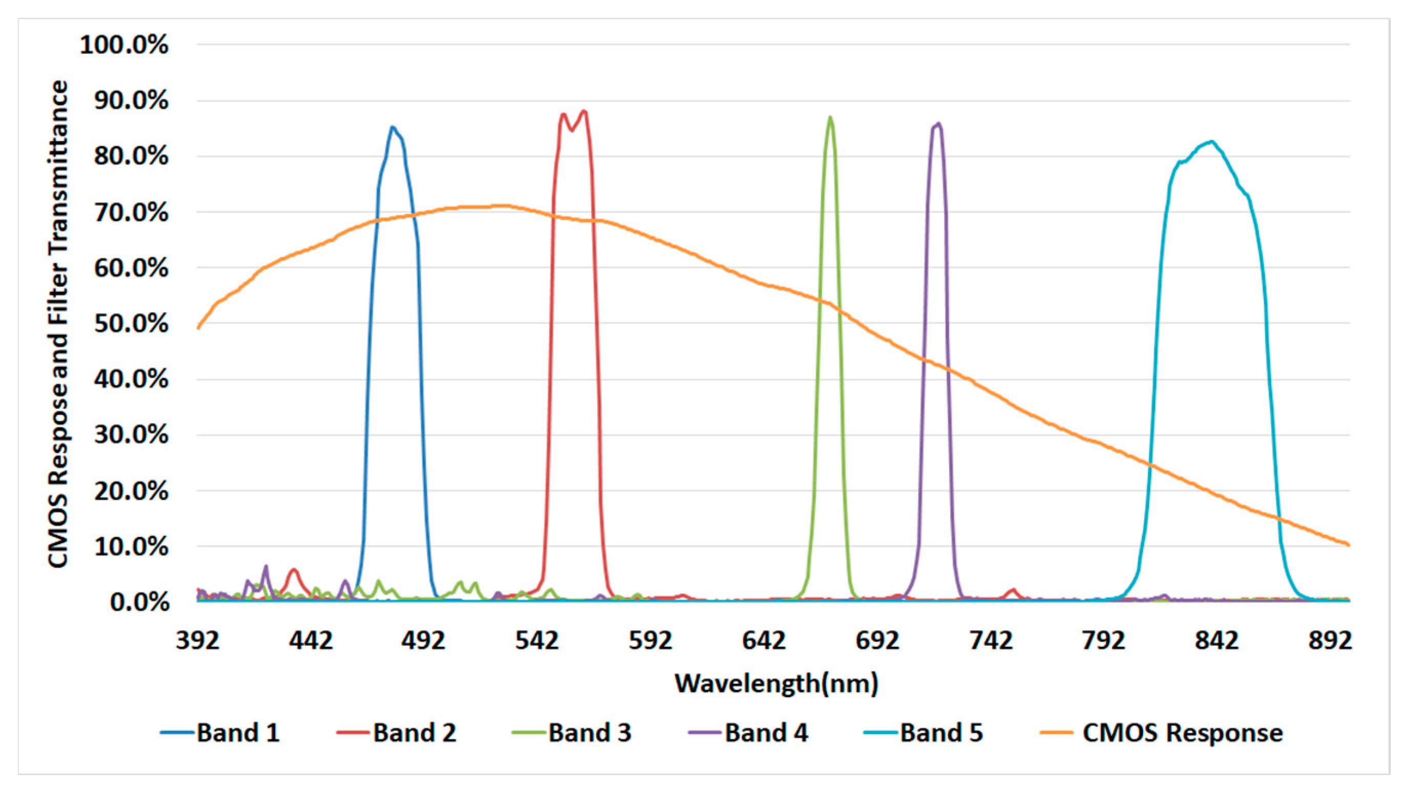
2.3. Experimental Schemes

The radiation calibration experiment was divided into three parts: dark current experiment, uniformity experiment, and absolute calibration experiment.

(1)

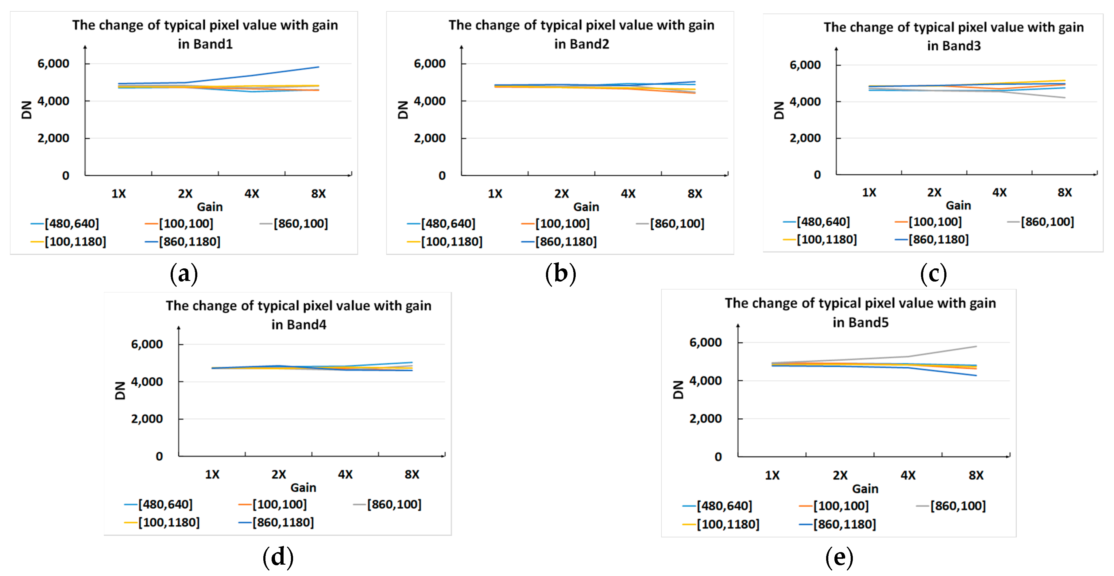
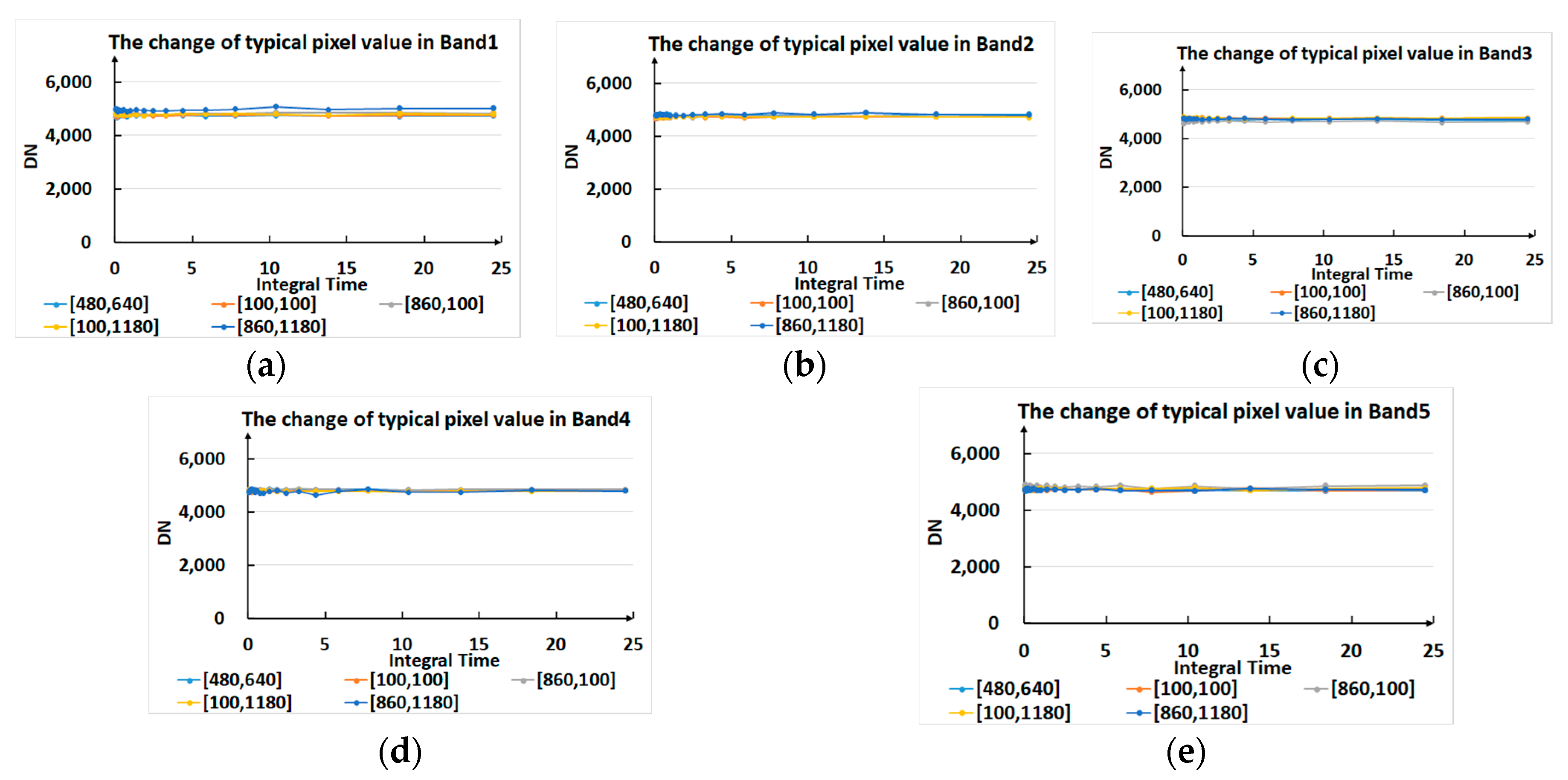
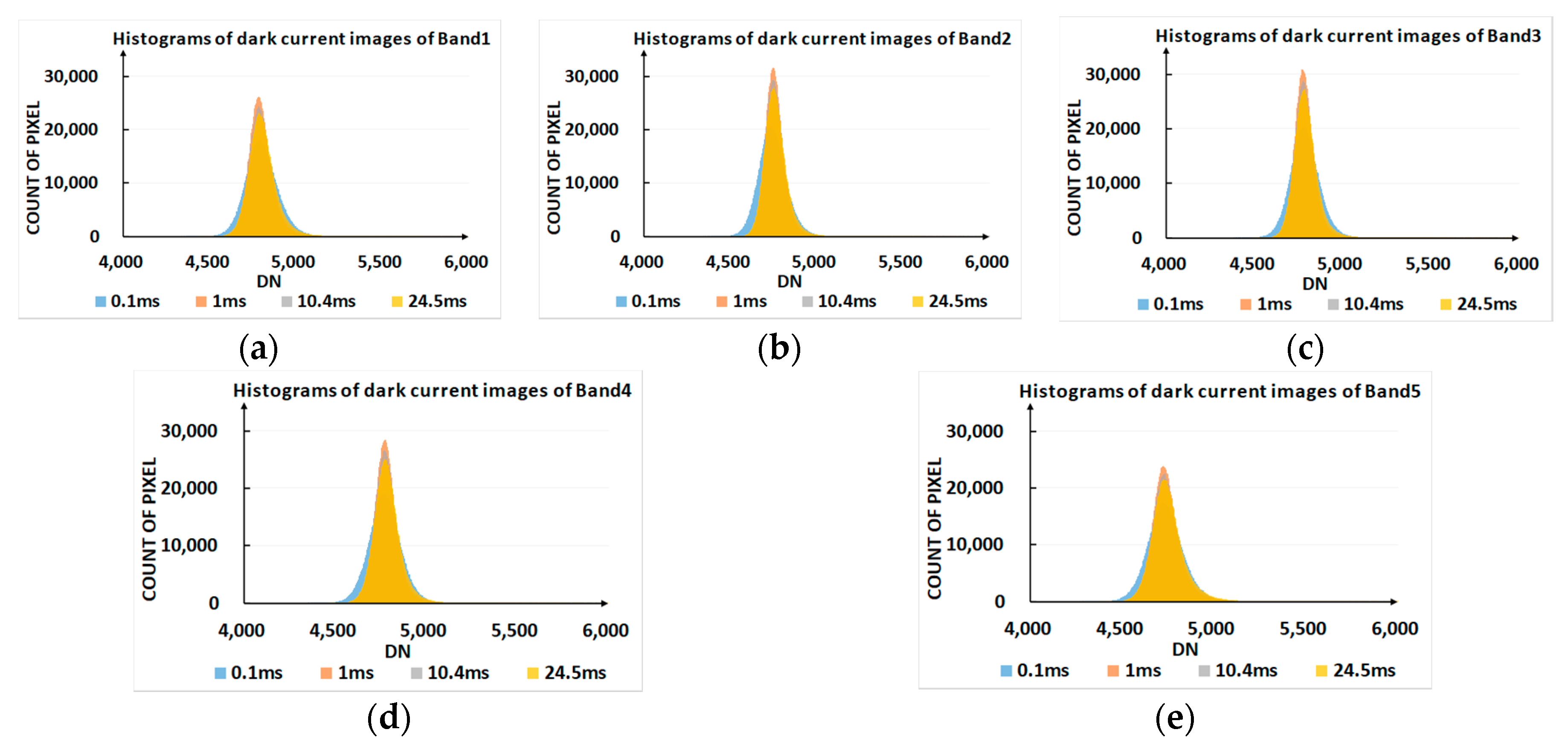
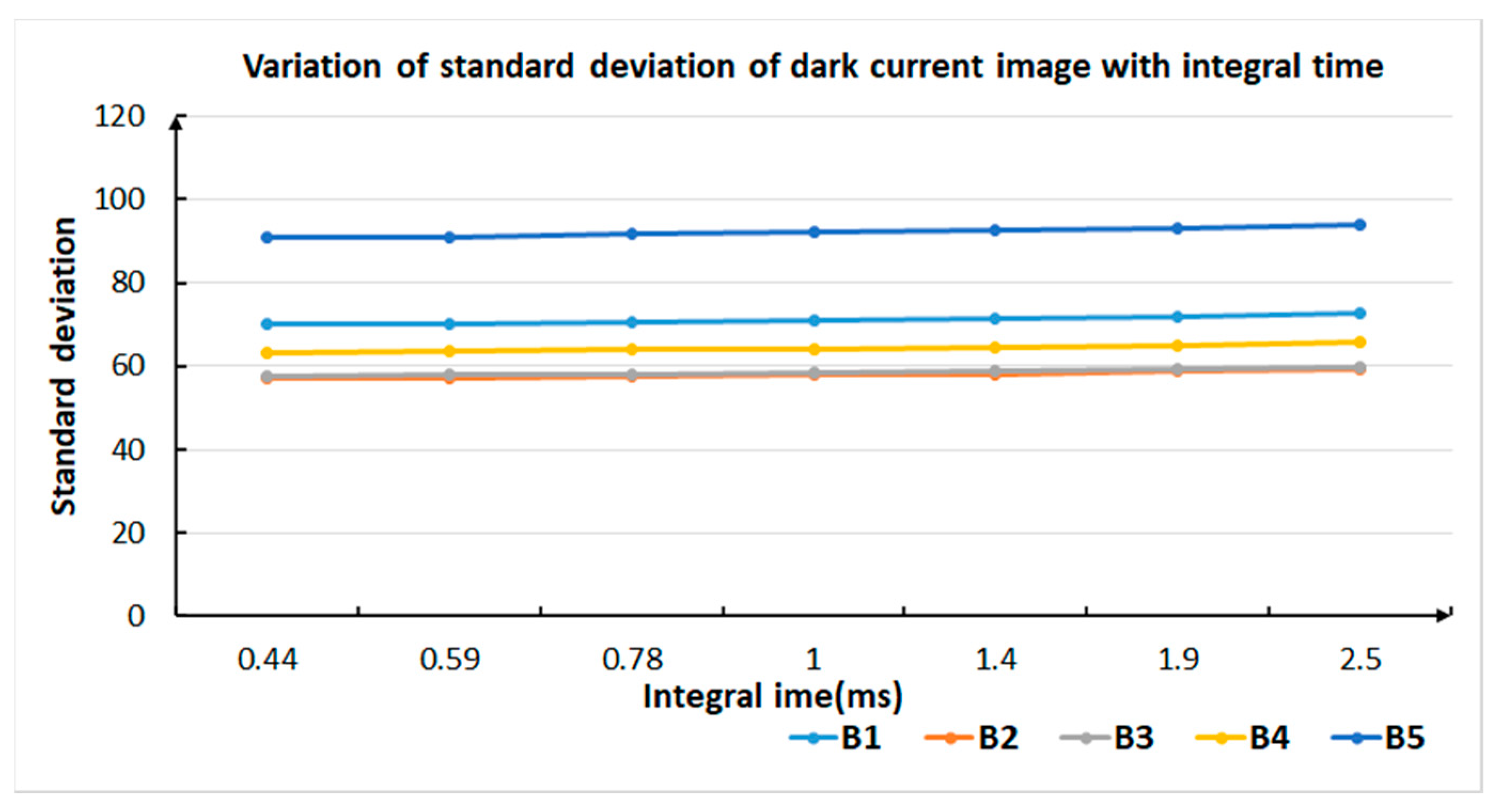
Dark current experiment: These experiments were conducted with a lens cover to simulate the environment without incident light. The variations in the dark current as a function of gain (1×, 2×, 4×, and 8×) and integration time (0.44, 0.59, 0.78, 1.0, 1.4, 1.9, and 2.5) were examined. Based on the method described in Section 2.2.2, the correction factor LUT for the non-uniformity of dark current was obtained.

(2)

Uniformity experiment: The quantized values of the image captured in the uniform light field of the integrating sphere were non-uniform due to the vignetting effect and differences in pixel response. Firstly, the dark current in the images was eliminated using the corresponding LUT. Then, the vignetting effect was analyzed based on Section 2.2.3. Subsequently, the difference in pixel response was examined using the images that had already been corrected for dark current and vignetting effect based on Section 2.2.4.

(3)

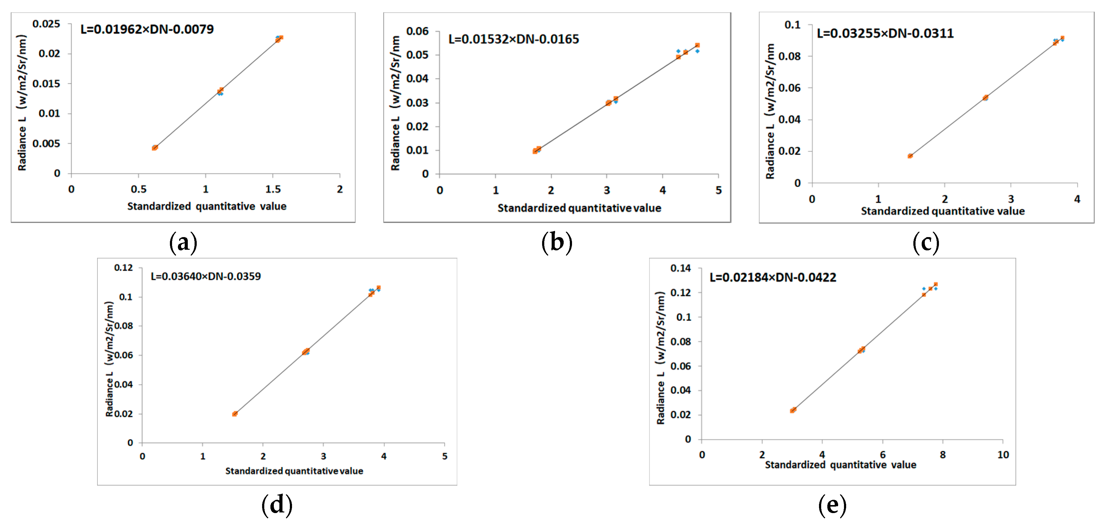
Absolute calibration experiment: The absolute calibration parameters were obtained through experiments with different output radiance levels of integrating sphere (100%, 70%, 40% output power) and integration times (0.44, 0.59, 0.78, 1.0, 1.4, 1.9, and 2.5 ms) of MicaSense RedEdge-MX. All the images were corrected for dark current, vignetting effect, and response according to the previous two steps. Then, the average value of the image was calculated as the effective quantized value to establish a linear relationship with incident radiance by linear regression.

The detailed experimental scheme is shown in Figure 4. In the experiment, the images were collected in 16-bit TIFF format, and the spectral radiance of the integrating sphere was recorded synchronously. The data were processed using MATLAB R2019a software (The MathWorks, Inc., Natick, MA, USA).

3. Experiments and Results

3.1. Results of Radiometric Calibration

3.1.1. Correction of Dark Current

To extract an optimal template image of dark current, dark current was analyzed in terms of gain and integration time. The representative pixel values and gray histogram were used to analyze the characteristics of images with dark current. The positions of five pixels in the images were extracted as typical pixel positions to analyze the characteristics: [x,y-480,640], [x,y-100,100], [x,y-860,100], [x,y-100,1180], and [x,y-860,1180]. The positions of five typical pixels were evenly distributed in the middle and four corners of the image. Gray histogram reflects the statistical characteristics of image pixels.

It is clear from Figure 5 that the DN of typical pixels did not increase with the increase in gain. Actually, there were no obvious changes in the dark current value of typical pixels for gain below 2×. The dark current values of the pixels were different when the gain was set to 4× and 8×. The value of some pixels increased, while that of other pixels decreased.

Figure 6 shows the statistical characteristics of dark current images. As the gain changed, the histogram of the dark current image appeared obviously different. The larger the gain, the more inconsistent the dark current value. Thus, to limit the effect of noise, the gain of the sensor should be set to a low level of 1× or 2× in practice.

The influence of gain and integration time (0.44–2.5 ms) on the dark current was experimentally analyzed, and the corresponding results are shown in Figure 7 and Figure 8, respectively. It is clear from Figure 7 that the dark current value of typical pixels in each band did not change with the increase in integration time. This suggested that the image template obtained at any integration time could be used to correct the dark current of the image captured at other integration time settings.

The histograms of dark current images were slightly changed under different values of integration time. To clearly display the statistical features of images, the standard deviation (STD) of the dark current image was selected to quantify this change. The STD of the dark current image in the integration time range of 0.44–2.5 ms, which is typically used for a multispectral camera in aviation applications, was statistically analyzed, and the results are shown in Figure 9.

From an integration time in the range of 0.44–2.5 ms, the STD was negligibly changed. This indicated there was no difference in the dark current of images captured between 0.44 and 2.5 ms.

The above experimental analysis provided guidance for selecting a representative dark current image as the correction factor LUT of $\mathrm{Dark}\left(x,y\right)$. Besides, the integration time of 1 ms is commonly used in practical application as it lies in the typical range used for aerial photography [19,22,33]. Consequently, the LUT of dark current $\mathrm{Dark}\left(x,y\right)$ in the radiometric calibration model was programmed as a typical image, which was the average of multiple images captured using gain of 1× and integration time of 1 ms.

3.1.2. Vignetting Effect

The vignetting effect of the image in which the effect of dark current had been eliminated is shown in Figure 10. The DN value decreased from the middle to the edge in the images captured by looking at the pupil of the integrating sphere, which output a uniform light field. Due to the vignetting effect, the edge brightness of the image was roughly 0.60–0.77 times the middle brightness in all the bands. The maximum luminance difference was 0.60 times in Band 5.

Based on Equations (5) and (6), the Gaussian filter template was created by inputting the appropriate STD $\mathsf{\sigma }$. The convolution algorithm was used between the $image$ and Gaussian filter ($filte{r}_{gsussian})$ template to generate the vignetting images. The fitting performance of all the bands are shown in Figure 11.

Then, the correction factor LUT of the vignetting effect was obtained by normalizing these images according to Equation (7). The normalized LUT of the vignetting effect of all the bands are displayed in Figure 12.

The correction factor LUT of the vignetting effect was used for image correction, and the results are shown in Figure 13. Compared to Figure 10, the brightness of the corrected image was even, which proved that the vignetting effect was eliminated.

3.1.3. Response Correction

The images obtained under the same output radiation intensity of the integration sphere and camera settings were corrected for dark current and vignetting effect. Their mean image was calculated to eliminate the random noise. The response differences that were retained in the images are shown in Figure 14. An obvious stripe noise was observed in the images of each band.

According to Equation (8), the correction factor LUT of the response function was calculated, which was then used to correct the images that were already corrected for dark current and vignetting effect. The results are shown in Figure 15.

The results suggested that DN values of images with response factor correction became smoother and more compact than before. This indicated that the difference in response between pixels had been effectively corrected. In the residual error, random noise was the main component.

3.1.4. Absolute Calibration Parameters

We collected 21 groups of data for each band. The datasets were measured under three incident brightness levels (the output power of the integrating sphere was 100%, 70%, and 40%) and seven integration times (0.44, 0.59, 0.78, 1.0, 1.4, 1.9, and 2.5 ms). The gain was set to 1×. Each group of data included five images captured continuously under the same condition. Five images in one group were averaged as one image to eliminate the random noise. Thus, 21 effective images were used for absolute radiometric calibration processing. The process is described as follows:

●

Firstly, according to Equation (2), all the collected images were corrected for dark current, vignetting effect, and non-uniform pixel response with the LUTs derived above.

●

Secondly, according to Equation (3), the 21 images were normalized with respect to the integration time, gain, and digital bit rate, and the mean DN was calculated for each corrected image.

●

Finally, the parameters of absolute radiometric calibration, i.e., $a\mathrm{and}b$, were obtained by least-squares fitting based on the mean DN of 21 corrected images and the spectral radiance output of the integration sphere [6,18,33].

The linear fitting results are shown in Figure 16, which proved the linear relationship between the data and radiance. The coefficient a, offset b, R-square, root mean square error (RMSE) and mean square (MS) of residual of linear fitting are displayed in

Table 2. Coefficient a, offset b, R-square, RMSE, and MS of residual of linear fitting.

Parameters Band	a	b	R-Square	RMSE	MS of Residual
Band1	0.01962	−0.0079	0.998	0.00041	1.68 × 10−7
Band2	0.01532	−0.0165	0.993	0.00159	2.53 × 10−6
Band3	0.03255	−0.0311	0.998	0.00140	1.95 × 10−6
Band4	0.03640	−0.0359	0.997	0.00175	3.06 × 10−6
Band5	0.02184	−0.0422	0.996	0.00260	6.74 × 10−6

. The R-squares of all the bands were remarkably close to 1, and the MS of residual of all the bands were close to 0. This indicated that the forecast precision of linear precision was good. In other words, the obtained values of coefficient a and offset b in absolute calibration were valid.

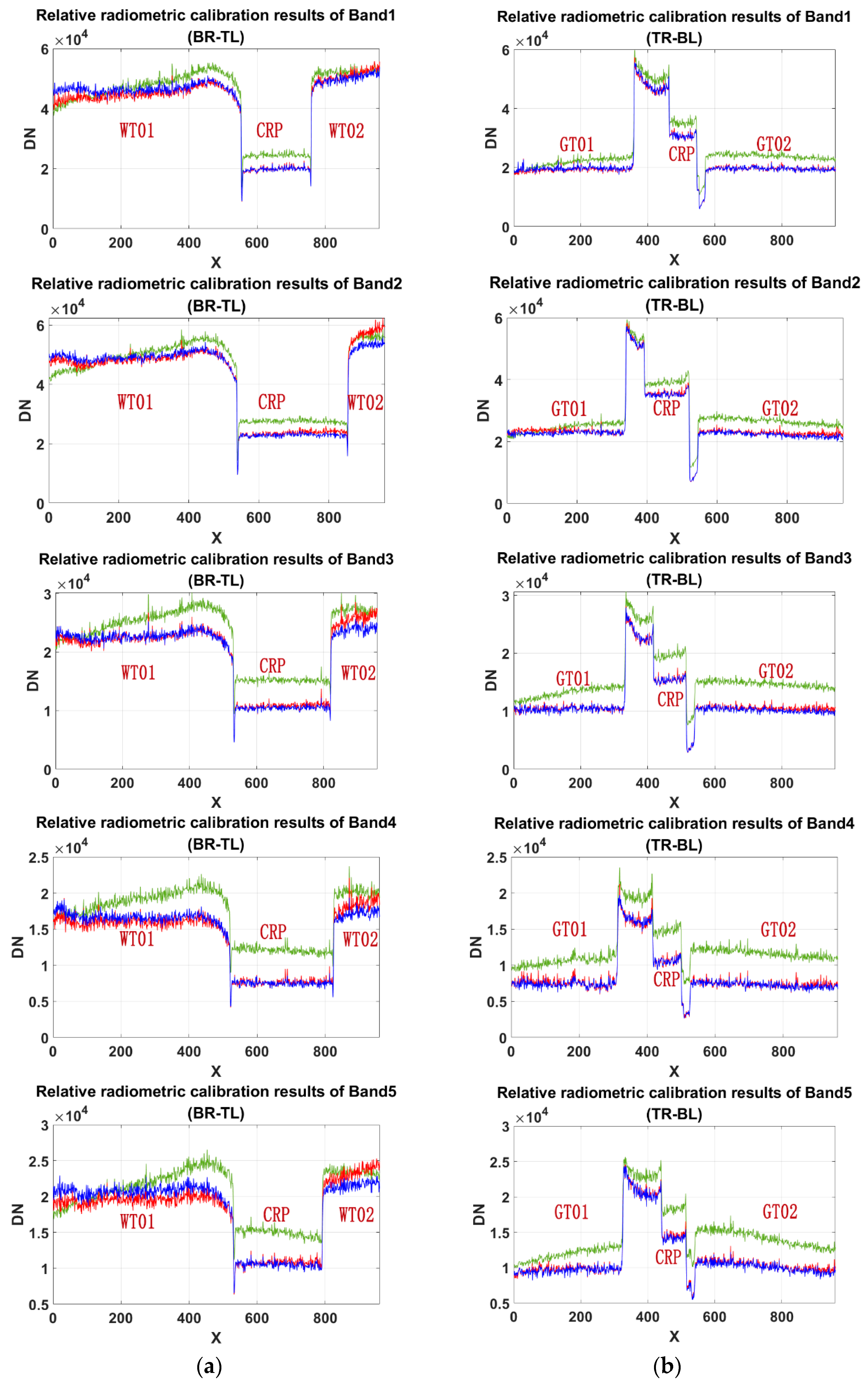
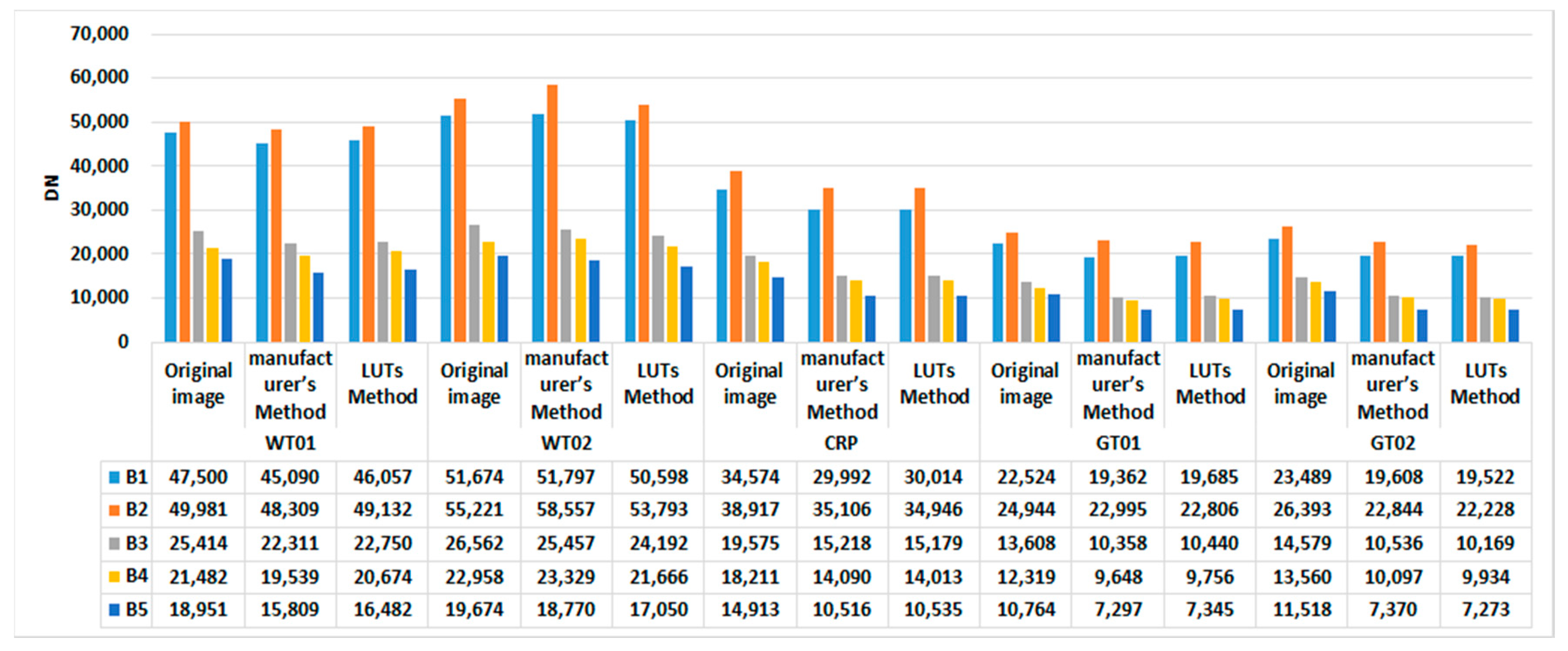
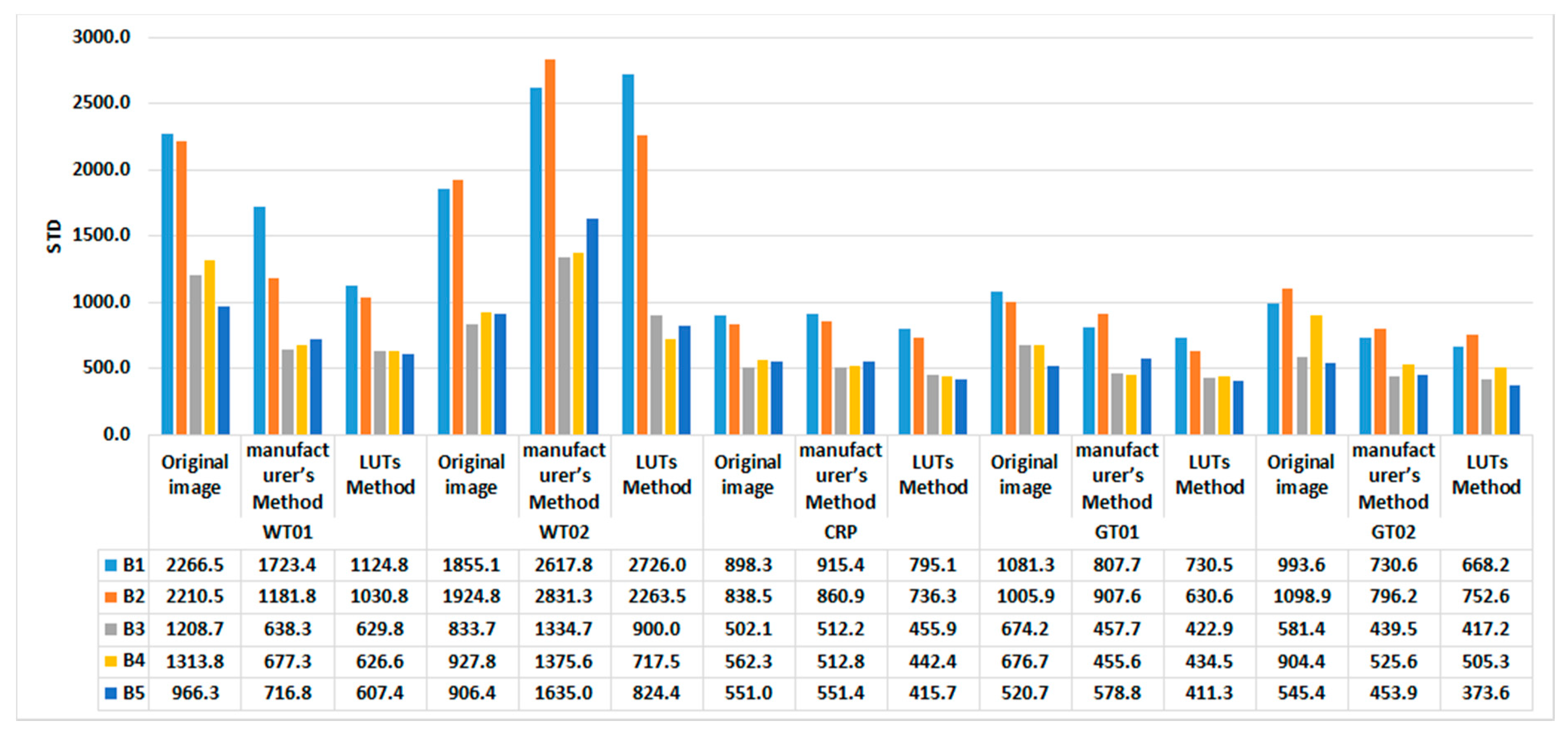
3.2. Verification of Results

3.2.1. Verification Method

To verify the effectiveness of the proposed radiometric calibration model, the relative accuracy and absolute accuracy of the model were evaluated. The relative accuracy was used to validate the uniformity of the corrected image, while the absolute accuracy was used to validate the radiance in images.

Five observation targets were combined: calibrated reflectance panels (CRP) provided by the manufacturer, white target01 (WT01), white target02 (WT02), gray target01 (GT01), and gray target02 (GT02). As shown in Figure 17a, the observation targets were arranged on flat ground.

The reflectance of five targets was measured using a RS-8800 field spectrometer (Spectral Evolution, USA) with a spectral range of 350–2500 nm. The target was observed from multiple angles. The average reflectance obtained through multi-angle observations was considered as an effective reflectance. The reflectance of targets at the spectral bands consistent with the center wavelength of RedEdge-MX are shown in

Table 3. Reflectance of five reference targets.

Band	WT01 (%)	WT02 (%)	CRP (%)	WT01 (%)	WT02 (%)
Band1	85.2	85.2	53.8	32.3	32.3
Band2	77.7	77.7	53.8	30.7	30.7
Band3	81.5	81.5	53.6	30.9	30.9
Band4	82.3	82.3	53.1	31.6	31.6
Band5	84.4	84.4	53.5	30.8	30.8

.

The experiment was conducted outdoors in cloudless conditions. According to the experimental scheme shown in Figure 17b, five spectral images were captured using a Mica Rededge-MX multispectral camera fixed on a tripod with a height of 1.5 m from the target such that the viewing angle was perpendicular to the ground. The Band1 image of targets is shown in Figure 18a as an example. The diagonal pixels are extracted in Figure 18b. The two diagonals selected were bottom right-top left (BR-TL) and top right-bottom left (TR-BL).

Further, the radiometric calibration method provided by the manufacturer of Rededge-MX [41] was also used to correct the same data and compared it with the proposed LUT-based method. The comparison results are discussed in the following subsections.

3.2.2. Relative Accuracy

After relative correction, the result was analyzed from three aspects: diagonal pixels of images, mean DN of targets, and STD of DN of targets. It was expected that the values of pixels should be more balanced than before in a single target and between similar targets. Firstly, the diagonal pixels of original images and the images corrected by two methods were extracted, and the corresponding results are shown in Figure 19.

It is clear from Figure 19 that the diagonal pixels of all the spectral images corrected by the two methods were smaller than that of the original spectral images because the dark current was eliminated. For one target, the pixels were flatter in the images corrected by the two methods. For similar targets, the consistency of DN values was also improved. In addition, Figure 19b shows that the effect of the two methods was roughly similar. However, the flatness of the pixel curve corrected by the LUT method was better than that of the curve corrected by the manufacturer’s method for the WT01 target and WT02 target and between them. This implied that the proposed LUT method facilitated better relative calibration than the manufacturer’s method.

For quantitative comparison, the mean and STD of DN of each observed targets in the original images and corrected images based on the two calibration methods are shown in Figure 20 and Figure 21.

It is evident from Figure 20 that the interval between the mean of the DN of WT01 and that of WT02 in the corrected results increased as compared to that in the original images. This may be attributed to the tilt observed by the sensor. However, the mean of DN of other similar targets became closer than before. This indicated the effectiveness of the two calibration methods. Moreover, the mean DN of all the same targets corrected by the LUT method was more uniform than that of the same targets corrected by the manufacturer’s method, as shown in Figure 20. This implied that the effect of the LUT method was better than that of the manufacturer’s method.

The STD of the DN of the WT02 target in the corrected images based on the two methods was larger than that of the original images. This also indicated the problem of sensor tilt similar to Figure 19a and Figure 20. However, the STD of other targets became smaller than that in the original images. This confirmed that the uniformity of the image was improved. Besides, the STD of all the targets corrected by the LUT method was smaller than that of the targets corrected by the manufacturer’s method. This indicated that the images corrected by the LUT method had better uniformity than those corrected by the manufacturer’s method.

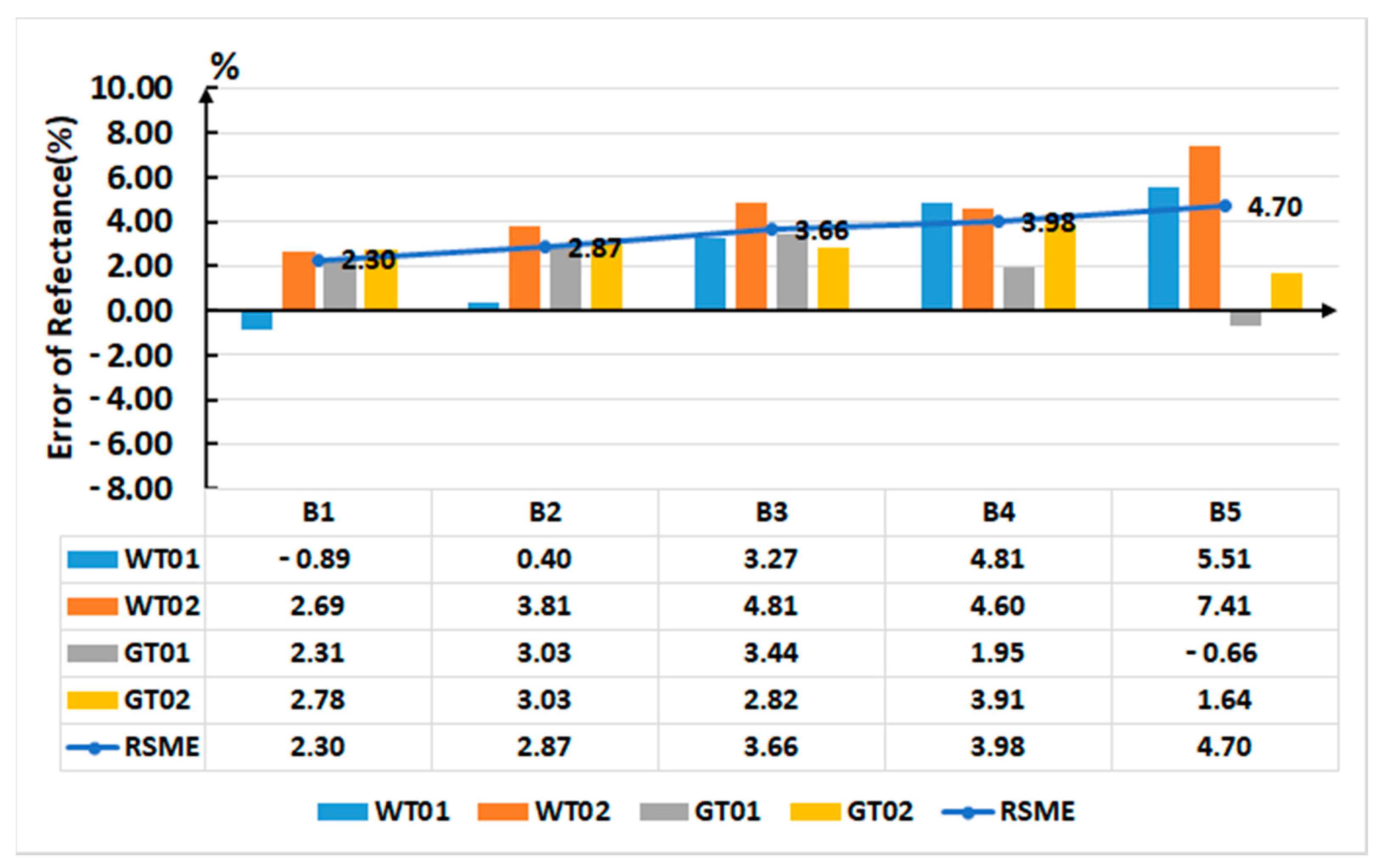
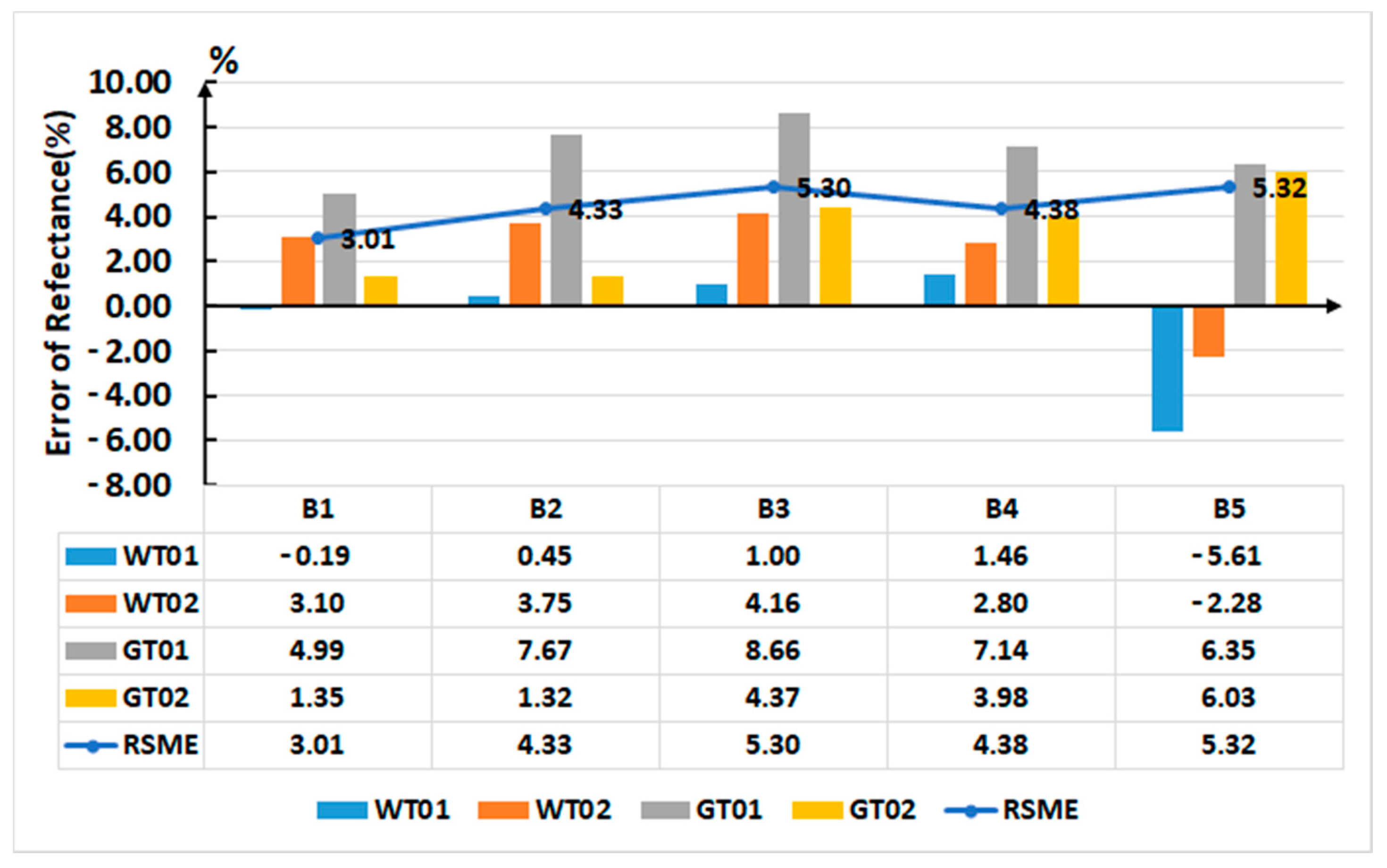
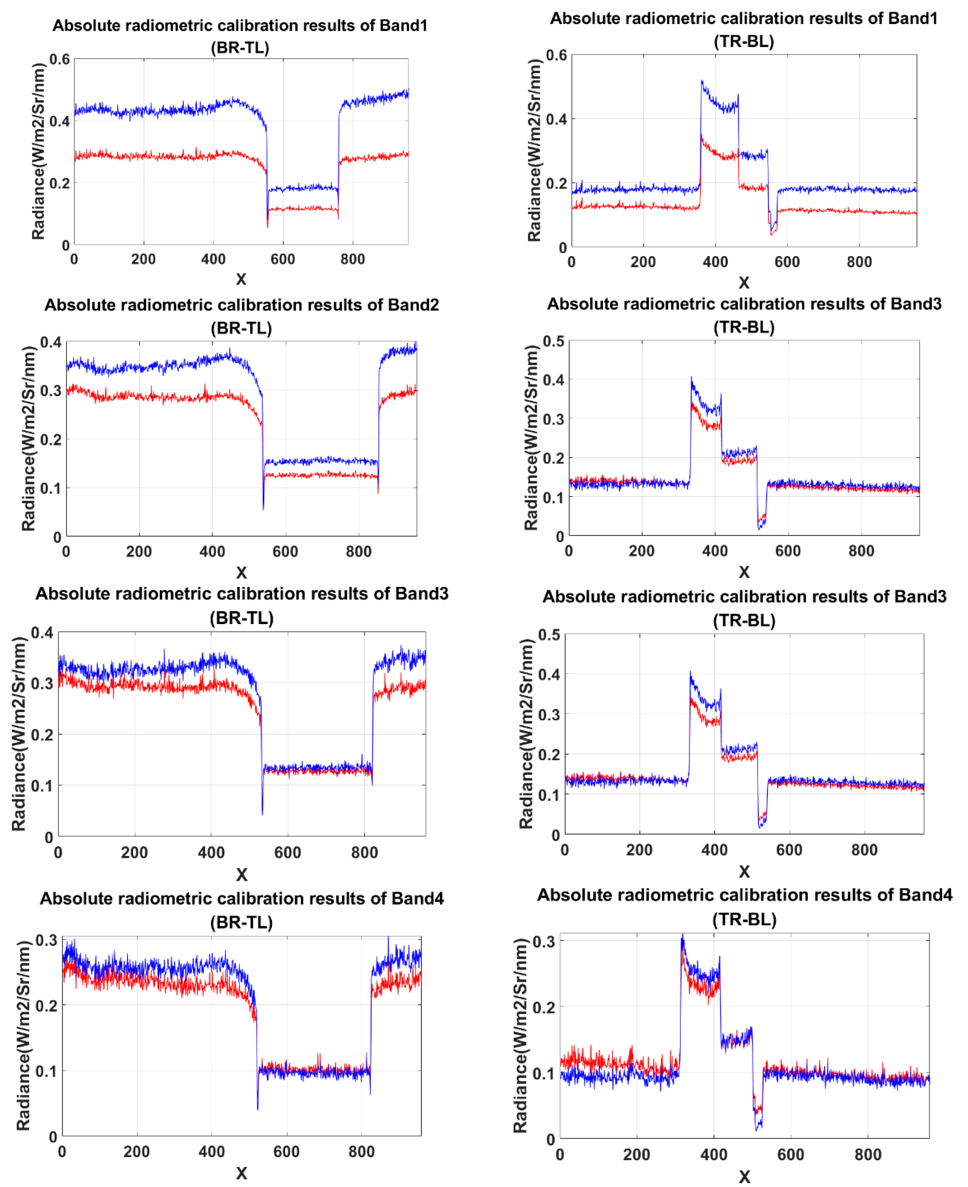
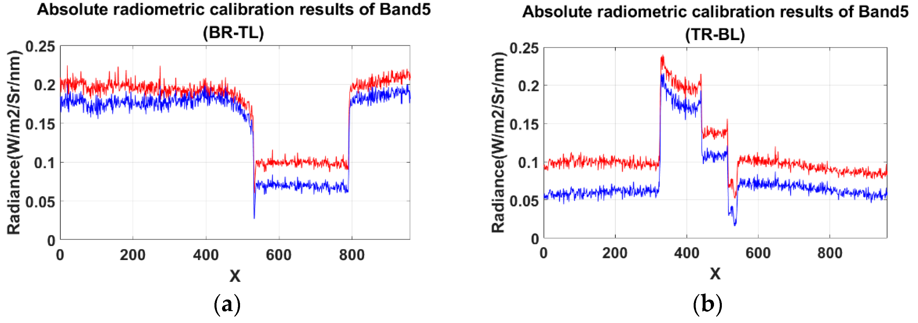
3.2.3. Absolute Accuracy

In practical applications, reflectance products are universally used for remote sensing analysis. In this study, a simple empirical model was used to convert the radiance of absolute radiometric calibration to reflectance [18,34]. Then, the reflectance of targets was compared with the actual reflectance measured by ASD to assess the absolute accuracy of the absolute radiometric calibration. CRP with better isotropy was selected as the known object. The equation was as follows:

$$imag{e}_{ref}^k=\frac{imag{e}_{cal-norm}^k}{{\rho }_{CRP}^k\ast CR{P}_{cal-norm}^k}$$

(11)

where $imag{e}_{cal-norm}^j$ was the $k$-band image, which had been corrected by absolute radiometric calibration; ${\rho }_{CRP}^k$ was the reflectance of CRP in $k$-band; $CR{P}_{cal-norm}^k$ was the average radiance of CRP in $imag{e}_{cal-norm}^j$; $imag{e}_{ref}^k$ was the reflectance of $k$-band image.

The absolute error of reflectance $\mathsf{\Delta }$ was defined as the difference between the actual reflectance $x_i^{\prime }$ of the radiation target $i$ and that measured by the sensor $x_i$. RMSE was used to evaluate the overall measurement accuracy of the sensors.

$$\mathsf{\Delta }=x_i-x_i^{\prime }$$

(12)

$$\mathrm{RMSE}=\sqrt{\frac{{\displaystyle \sum }{(x_i-x_i^{\prime })}^2}{N}}$$

(13)

The average reflectance of WT01, WT02, GT01, and GT02 was extracted from the reflectance images $imag{e}_{ref}^k$ calibrated by the LUT method and the manufacturer’s method. Then, the absolute error and RSME were calculated according to Equations (10) and (11). The reflectance error of targets in the five spectral images corrected by the LUT method and manufacturer’s method is shown in Figure 22 and Figure 23, respectively.

Comparing the data in Figure 22 and Figure 23, it was clear that the RMSE of reflectance of targets in the five spectral images corrected by the LUT method was less than that of spectral images corrected by the manufacturer’s method. The RMSE of reflectance calibrated using the proposed LUT method were 2.30%, 2.87%, 3.66%, 3.98%, and 4.70% for Band1, Band2, Band3, Band4, and Band5, respectively.

It should be noted that the normalization procedure of the calibration method provided by the manufacturer of the multispectral camera deteriorated the result, and the calibration parameter of integration time was not appropriate for the global shutter. Additionally, there was a systematic deviation between the radiance images of all the bands calculated by the two methods. This was probably because the performance of the sensor declined with use, and the absolute calibration coefficients measured before the delivery were unable to meet the current requirements. These two problems are shown in Figure 24.

Compared to Figure 19, there was a large deviation between the radiance value derived by two methods after normalization and absolute radiometric calibration. This is more obvious in the images of Band1 and Band2 in Figure 24. The curve of diagonal pixels is obviously raised on the left side and decreased on the right side in Figure 24b, reflecting the adverse effects of line correction of integration time in the manufacturer’s method.

4. Discussion

The radiometric calibration process of remote sensing instruments involves many aspects and is complex, especially for 2D image sensors. According to the comparison with the method provided by the manufacturer of the sensor, it was verified that the proposed radiometric calibration procedures based on the LUTs achieve encouraging results for Rededge-MX multispectral camera.

The dark current was characterized in terms of integration time and gain. This has rarely been attempted in previous studies. It was proved that compared to the mean value of the dark current image, the LUT of dark current is more appropriate for correcting the non-uniformity of dark current in the 2D image space. The effect of temperature was not considered in the dark current analysis as the inclusion of temperature can complicate the problem, and this will be discussed in future work. Dark current experiments were conducted after the device temperature was stabilized to room temperature. During the process of obtaining the normalized LUT of the vignetting effect, extracting the vignetting effect from images is a challenge, which is also the basis for eliminating the vignetting effect. The proposed method based on the Gaussian filter is simple and efficient, and it successfully eliminated the vignetting effect. Notably, this method is more effective for irregular or complex vignetting effect as shown in Band4 and Band5 of RedEdge-MX. The reliability of the results was verified from two aspects: relative accuracy and absolute accuracy, and comparison with the calibration method provided by the manufacturer of the spectral camera. In earlier studies, only one of the verification approaches has been commonly used [14,24,42]. This limits the wide utilization of sensors. On the other hand, the verification results of the proposed radiometric calibration model provided excellent relative accuracy and absolute accuracy.

Overall, the proposed radiometric calibration method based on LUTs provides outstanding results for complex and low-cost sensors. Because the basic principles of imaging sensors are similar, this method can also be used for sensors of the same type or for simple, advanced sensors such as the linear sensor or 2D-frame CCD sensor. This validates the universality of the proposed method. However, it may be noted that this experiment was implemented using an integration sphere in the laboratory environment. For field applications, the integration sphere may be replaced in the reflectance calibration procedures, but the experimental conditions need to be strictly controlled, including the uniformity of reflectance calibration, direction of sensor observation, interference from surrounding objects, etc. Accurate radiometric calibration of sensors is the basis of remote sensing. Accordingly, our future research will focus on radiation correction and widening the applications of the sensor.

5. Conclusions

In this study, a radiometric calibration model was proposed to determine the LUTs of correction factors for the dark current, vignetting effect, and non-uniform detection response and the absolute calibration parameters were also analyzed. The LUT of dark current correction was determined as the image template captured at a camera setting of 1× gain and 1 ms integration time. The LUT of the vignetting effect correction was obtained as the image with normalized brightness filtered by the Gaussian function. The LUT of the response correction was the ratio of the image value of each pixel to the mean value of the image obtained after correcting the dark current and vignetting effect. Then, the parameters of absolute calibration were derived by the linear fitting.

The LUTs of correction factors effectively improved the images. The absolute calibration parameters precisely converted the DN value to the radiance unit. The calibration accuracy of each band was evaluated by observing the reference targets and comparison with the method provided by the manufacturer of the sensor. The results revealed that the performance of the proposed radiometric calibration method based on LUTs was much better than that of the method provided by the manufacturer in terms of both relative accuracy and absolute accuracy. The RMSE of reflectance of reference targets derived from radiance images were 2.30%, 2.87%, 3.66%, 3.98%, and 4.70% for Band1, Band2, Band3, Band4, and Band5, respectively. Overall, the proposed LUT method based on the inherent characteristics of the image effectively realizes radiometric calibration of small multispectral cameras. The present results can serve as a useful reference for the improvement of multispectral cameras and boosting their practical applications.

References

1. Lebourgeois, V.; Bégué, A.; Labbé, S.; Mallavan, B.; Prévot, L.; Roux, B. Can commercial digital cameras be used as multispectral sensors? A crop monitoring test. Sensors 2008, 8, 7300–7322. [Google Scholar] [CrossRef] [PubMed]
2. Assmann, J.J.; Kerby, J.T.; Cunliffe, A.M.; Myers-Smith, I.H. Vegetation monitoring using multispectral sensors — best practices and lessons learned from high latitudes. J. Unmanned Veh. Syst. 2019, 7, 54–75. [Google Scholar] [CrossRef] [Green Version]
3. Pozo, S.D.; Rodríguez-Gonzálvez, P.; Hernández-López, D.; Felipe-García, B. Vicarious radiometric calibration of a multispectral camera on board an unmanned aerial system. Remote Sens. 2014, 6, 1918–1937. [Google Scholar] [CrossRef] [Green Version]
4. Hakala, T.; Markelin, L.; Honkavaara, E.; Scott, B.; Theocharous, T.; Nevalainen, O.; Näsi, R.; Suomalainen, J.; Viljanen, N.; Greenwell, C.; et al. Direct reflectance measurements from drones: Sensor absolute radiometric calibration and system tests for forest reflectance characterization. Sensors 2018, 18, 1417. [Google Scholar] [CrossRef] [PubMed] [Green Version]
5. Nocerino, E.; Dubbini, M.; Menna, F.; Remondino, F.; Gattelli, M.; Covi, D. Geometric calibration and radiometric correction of the maia multispectral camera. Int. Arch. Photogramm. Remote Sens. Spat. Inf. Sci.—ISPRS Arch. 2017, 42, 149–156. [Google Scholar] [CrossRef] [Green Version]
6. Markelin, L.; Suomalainen, J.; Hakala, T.; Oliveira, R.A.; Viljanen, N.; Näsi, R.; Scott, B.; Theocharous, T.; Greenwell, C.; Fox, N.; et al. Methodology for direct reflectance measurement from a drone: System description, radiometric calibration and latest results. Int. Arch. Photogramm. Remote Sens. Spat. Inf. Sci.—ISPRS Arch. 2018, 42, 283–288. [Google Scholar] [CrossRef] [Green Version]
7. Aasen, H.; Honkavaara, E.; Lucieer, A.; Zarco-Tejada, P.J. Quantitative remote sensing at ultra-high resolution with UAV spectroscopy: A review of sensor technology, measurement procedures, and data correctionworkflows. Remote Sens. 2018, 10, 1091. [Google Scholar] [CrossRef] [Green Version]
8. Feng, D.; Shi, B. Systematical approach for noise in CMOS LNA. Pan Tao Ti Hsueh Pao/Chin. J. Semicond. 2005, 26, 487–493. [Google Scholar]
9. Burke, B.; Jorden, P.; Paul, V.U. CCD technology. Exp. Astron. 2006, 19, 69–102. [Google Scholar] [CrossRef]
10. Hain, R.; Kähler, C.J.; Tropea, C. Comparison of CCD, CMOS and intensified cameras. Exp. Fluids 2007, 42, 403–411. [Google Scholar] [CrossRef]
11. Tian, H.; Fowler, B.; El Gamal, A. Analysis of temporal noise in CMOS photodiode active pixel sensor. IEEE J. Solid-State Circuits 2001, 36, 92–101. [Google Scholar] [CrossRef] [Green Version]
12. Honkavaara, E.; Khoramshahi, E. Radiometric correction of close-range spectral image blocks captured using an unmanned aerial vehicle with a radiometric block adjustment. Remote Sens. 2018, 10, 256. [Google Scholar] [CrossRef] [Green Version]
13. Moran, S.; Fitzgerald, G.; Rango, A.; Walthall, C.; Barnes, E.; Bausch, W.; Clarke, T.; Daughtry, C.; Everitt, J.; Escobar, D.; et al. Sensor development and radiometric correction for agricultural applications. Photogramm. Eng. Remote Sens. 2003, 69, 705–718. [Google Scholar] [CrossRef]
14. Olsen, D.; Dou, C.; Zhang, X.; Hu, L.; Kim, H.; Hildum, E. Radiometric calibration for AgCam. Remote Sens. 2010, 2, 464–477. [Google Scholar] [CrossRef] [Green Version]
15. Franz, M.O.; Grunwald, M.; Schall, M.; Laube, P.; Umlauf, G. Radiometric calibration of digital cameras using neural networks. In Optics and Photonics for Information Processing XI; International Society for Optics and Photonics: Bellingham, WA, USA, 2017. [Google Scholar] [CrossRef]
16. Bigas, M.; Cabruja, E.; Forest, J.; Salvi, J. Review of CMOS image sensors. Microelectron. J. 2006, 37, 433–451. [Google Scholar] [CrossRef] [Green Version]
17. Tagle Casapia, M.X. Study of radiometric variations in Unmanned Aerial Vehicle remote sensing imagery for vegetation mapping. Lund Univ. GEM Thesis Ser. 2017. [Google Scholar] [CrossRef]
18. Duan, Y.; Yan, L.; Yang, B.; Jing, X.; Chen, W. Outdoor relative radiometric calibration method using gray scale targets. Sci. China Technol. Sci. 2013, 56, 1825–1834. [Google Scholar] [CrossRef]
19. Minařík, R.; Langhammer, J.; Hanuš, J. Radiometric and atmospheric corrections of multispectral μMCA Camera for UAV spectroscopy. Remote Sens. 2019, 11, 2428. [Google Scholar] [CrossRef] [Green Version]
20. Aasen, H.; Bendig, J.; Bolten, A.; Bennertz, S.; Willkomm, M.; Bareth, G. Introduction and preliminary results of a calibration for full-frame hyperspectral cameras to monitor agricultural crops with UAVs. Int. Arch. Photogramm. Remote Sens. Spat. Inf. Sci.—ISPRS Arch. 2014, 40, 1–8. [Google Scholar] [CrossRef] [Green Version]
21. Suomalainen, J.; Anders, N.; Iqbal, S.; Roerink, G.; Franke, J.; Wenting, P.; Hünniger, D.; Bartholomeus, H.; Becker, R.; Kooistra, L. A lightweight hyperspectral mapping system and photogrammetric processing chain for unmanned aerial vehicles. Remote Sens. 2014, 6, 11013–11030. [Google Scholar] [CrossRef] [Green Version]
22. Aasen, H.; Burkart, A.; Bolten, A.; Bareth, G. Generating 3D hyperspectral information with lightweight UAV snapshot cameras for vegetation monitoring: From camera calibration to quality assurance. ISPRS J. Photogramm. Remote Sens. 2015, 108, 245–259. [Google Scholar] [CrossRef]
23. Minařík, R.; Langhammer, J. Rapid radiometric calibration of multiple camera array using insitu data for UAV multispectral photogrammetry. Int. Arch. Photogramm. Remote Sens. Spat. Inf. Sci.—ISPRS Arch. 2019, 42, 209–215. [Google Scholar] [CrossRef] [Green Version]
24. Kelcey, J.; Lucieer, A. Sensor correction of a 6-band multispectral imaging sensor for UAV remote sensing. Remote Sens. 2012, 4, 1462–1493. [Google Scholar] [CrossRef] [Green Version]
25. Shin, J.; Sakurai, T. The Vignetting Effect of the Soft X-Ray Telescope Onboard Yohkoh: II. Pre-Launch Data Analysis. Sol. Phys. 2016, 291, 705–725. [Google Scholar] [CrossRef]
26. He, K.; Zhao, H.Y.; Liu, J.J. Vignetting correction method for aviatic remote sensing image. Jilin Daxue Xuebao (Gongxueban)/J. Jilin Univ. (Eng. Technol. Ed.) 2007, 37, 1447–1450. [Google Scholar] [CrossRef]
27. Lou, Z.; Li, T.; Shen, S. Vignetting correction method for the infrared system based on polynomial approximation. Infrared Laser Eng. 2016, 45, 6–10. [Google Scholar]
28. Ortega-Terol, D.; Hernandez-Lopez, D.; Ballesteros, R.; Gonzalez-Aguilera, D. Automatic hotspot and sun glint detection in UAV multispectral images. Sensors 2017, 17, 2352. [Google Scholar] [CrossRef] [Green Version]
29. Honkavaara, E.; Hakala, T.; Markelin, L.; Rosnell, T.; Saari, H.; Mäkynen, J. A process for radiometric correction of UAV image blocks. Photogramm. Fernerkundung Geoinf. 2012, 2012, 115–127. [Google Scholar] [CrossRef]
30. Yu, W.; Chung, Y.; Soh, J. Vignetting distortion correction method for high quality digital imaging. Proc. Int. Conf. Pattern Recognit. 2004, 3, 666–669. [Google Scholar] [CrossRef]
31. Mamaghani, B.; Salvaggio, C. Multispectral sensor calibration and characterization for sUAS remote sensing. Sensors 2019, 19, 4453. [Google Scholar] [CrossRef] [Green Version]
32. MicaSense. RedEdge-MX. Available online: https://www.micasense.com/rededge-mx/ (accessed on 14 October 2020).
33. Li, X.; Gao, H.; Yu, C.; Chen, Z.C. Impact analysis of lens shutter of aerial camera on image plane illuminance. Optik (Stuttg) 2018, 173, 120–131. [Google Scholar] [CrossRef]
34. Lin, D.; Maas, H.G.; Westfeld, P.; Budzier, H.; Gerlach, G. An advanced radiometric calibration approach for uncooled thermal cameras. Photogramm. Rec. 2018, 33, 30–48. [Google Scholar] [CrossRef]
35. Tu, Y.H.; Phinn, S.; Johansen, K.; Robson, A. Assessing radiometric correction approaches for multi-spectral UAS imagery for horticultural applications. Remote Sens. 2018, 10, 1684. [Google Scholar] [CrossRef] [Green Version]
36. Wang, C.; Myint, S.W. A Simplified Empirical Line Method of Radiometric Calibration for Small Unmanned Aircraft Systems-Based Remote Sensing. IEEE J. Sel. Top. Appl. Earth Obs. Remote Sens. 2015, 8, 1876–1885. [Google Scholar] [CrossRef]
37. Bedrich, K.; Bokalic, M.; Bliss, M.; Topic, M.; Betts, T.R.; Gottschalg, R. Electroluminescence Imaging of PV Devices: Advanced Vignetting Calibration. IEEE J. Photovoltaics 2018, 8, 1297–1304. [Google Scholar] [CrossRef] [Green Version]
38. Zheng, Y.; Lin, S.; Kambhamettu, C.; Yu, J.; Kang, S.B. Single-image vignetting correction. IEEE Trans. Pattern Anal. Mach. Intell. 2009, 31, 2243–2256. [Google Scholar] [CrossRef]
39. Wang, L.; Suo, J.; Fan, J. Spatialoral codec accuracy calibration for multi-scale giga-pixel macroscope. In Proceedings of the 2019 IEEE International Conference on Multimedia & Expo Workshops (ICMEW), Shanghai, China, 8–12 July 2019; pp. 414–419. [Google Scholar] [CrossRef]
40. Aggarwal, M.; Hua, H.; Ahuja, N. On cosine-fourth and vignetting effects in real lenses. Proc. IEEE Int. Conf. Comput. Vis. 2001, 1, 472–479. [Google Scholar] [CrossRef]
41. MicaSense. RedEdge-MX. Available online: https://support.micasense.com/hc/en-us/articles/115000351194-RedEdge-Camera-Radiometric-Calibration-Model (accessed on 14 October 2020).
42. Lu, Y.; Wang, K.; Fan, G. Photometric calibration and image stitching for a large field of view multi-camera system. Sensors 2016, 16, 516. [Google Scholar] [CrossRef] [Green Version]
Figure 1. Filter transmittance for each band and spectral response of complementary metal-oxide semiconductor (CMOS) in MicaSense RedEdge-MX.
Remotesensing 12 04012 g001
Figure 2. Integrating sphere system: (a) structure of integrating sphere system; (b) observation scheme of calibration.
Remotesensing 12 04012 g002
Figure 3. Workflow to obtain the lookup table (LUT) of dark current and dark current correction.
Remotesensing 12 04012 g003
Figure 4. Workflow of radiation calibration experiment.
Remotesensing 12 04012 g004
Figure 5. Variation in the typical pixel value with gain for: (a) Band1; (b) Band2; (c) Band3; (d) Band4; (e) Band5.
Remotesensing 12 04012 g005
Figure 6. Histograms of dark current images at different gain settings for various bands: (a) Band1; (b) Band2; (c) Band3; (d) Band4; (e) Band5.
Remotesensing 12 04012 g006
Figure 7. Variation in the typical pixel value as a function of integration time for various bands: (a) Band1; (b) Band2; (c) Band3; (d) Band4; (e) Band5.
Remotesensing 12 04012 g007
Figure 8. Histograms of dark current images at different integration times (0.1, 1.0, 10.4, and 24.5 ms) for various bands: (a) Band1; (b) Band2; (c) Band3; (d) Band4; (e) Band5.
Remotesensing 12 04012 g008
Figure 9. Variation in the standard deviation of the dark current image with integration time (0.44–2.5 ms).
Remotesensing 12 04012 g009
Figure 10. Vignetting effect: (a) vignetting of images of Band1-Band5; (b) vignetting of middle row pixels in the images of Band1–Band5.
Remotesensing 12 04012 g010aRemotesensing 12 04012 g010b
Figure 11. Comparison of middle row pixels between vignetting image and original image: (a) fitting performance of Band1; (b) fitting performance of Band2; (c) fitting performance of Band3; (d) fitting performance of Band4; (e) fitting performance of Band5.
Remotesensing 12 04012 g011
Figure 12. Normalized LUT of vignetting coefficient: (a) normalized LUT of Band1; (b) normalized LUT of Band2; (c) normalized LUT of Band3; (d) normalized LUT of Band4; (e) normalized LUT of Band5.
Remotesensing 12 04012 g012
Figure 13. Results of vignetting correction for various band images: (a) Band1 image; (b) Band2 image; (c) Band3 image; (d) Band4 image; (e) Band5 image.
Remotesensing 12 04012 g013
Figure 14. Response noise of band images corrected for dark current and vignetting effect: (a) Band1 image; (b) Band2 image; (c) Band3 image; (d) Band4 image; (e) Band5 image.
Remotesensing 12 04012 g014
Figure 15. Comparison of response correction between (a) the images corrected for dark current and vignetting effect but not for the non-uniform response (Band1-Band5) and (b) the images are corrected for dark current, vignetting effect, and non-uniform response (Band1-Band5).
Remotesensing 12 04012 g015aRemotesensing 12 04012 g015b
Figure 16. Linear fitting results for different bands: (a) Band1; (b) Band2; (c) Band3; (d) Band4; (e) Band5.
Remotesensing 12 04012 g016
Figure 17. Verification experiments: (a) layout of observation targets; (b) schematic of the experimental setup.
Remotesensing 12 04012 g017
Figure 18. Images obtained by the multispectral camera (Band1 as an example): (a) Band1 image of targets; (b) diagonal pixels of five spectral images selected for relative accuracy; (c) areas selected for analyzing pixel statistics of images.
Remotesensing 12 04012 g018
Figure 19. Comparison of diagonal pixels of original images and the images corrected by two methods (green-original images, red-manufacturer’s method, blue-proposed LUT method): (a) BR-TL diagonal pixels of five bands; (b) TR-BL diagonal pixels of five bands.
Remotesensing 12 04012 g019
Figure 20. Mean digital number (DN) of five targets in the original image and the images corrected by the two calibration methods.
Remotesensing 12 04012 g020
Figure 21. STD of DN of targets in the original image and image corrected by the two calibration methods.
Remotesensing 12 04012 g021
Figure 22. Error of reflectance of targets in five spectral images corrected by the LUT method.
Remotesensing 12 04012 g022
Figure 23. Error of reflectance of targets in five spectral images corrected by the manufacturer’s method.
Remotesensing 12 04012 g023
Figure 24. Diagonal radiance value of the spectral images calibrated by the LUT method (blue) and manufacturer’s method (red): (a) radiance value of BR-TL diagonal in five bands; (b) radiance value of TR-BL diagonal in five bands.
Remotesensing 12 04012 g024aRemotesensing 12 04012 g024b