Earth Observation Data Cubes for Brazil: Requirements, Methodology and Products

 , , ,
, , ,  ,
,  , ,
, ,  , ,
, ,  , , , , ,
  and
and
Abstract
:
1. Introduction
2. Requirements for EO Data Cubes for Brazil
2.1. Image Time Series Analysis and Machine Learning
2.2. ARD and Data Cubes of Medium-Resolution Satellite Images
2.3. Land Use and Cover Samples and Data Sets
2.4. Interoperability and Web Services
2.5. Cloud Computing and Distributed Processing Environments
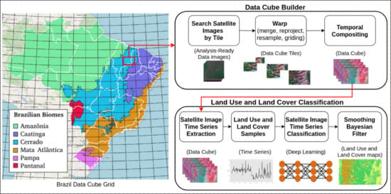
3. Methodology for EO Data Cube Generation
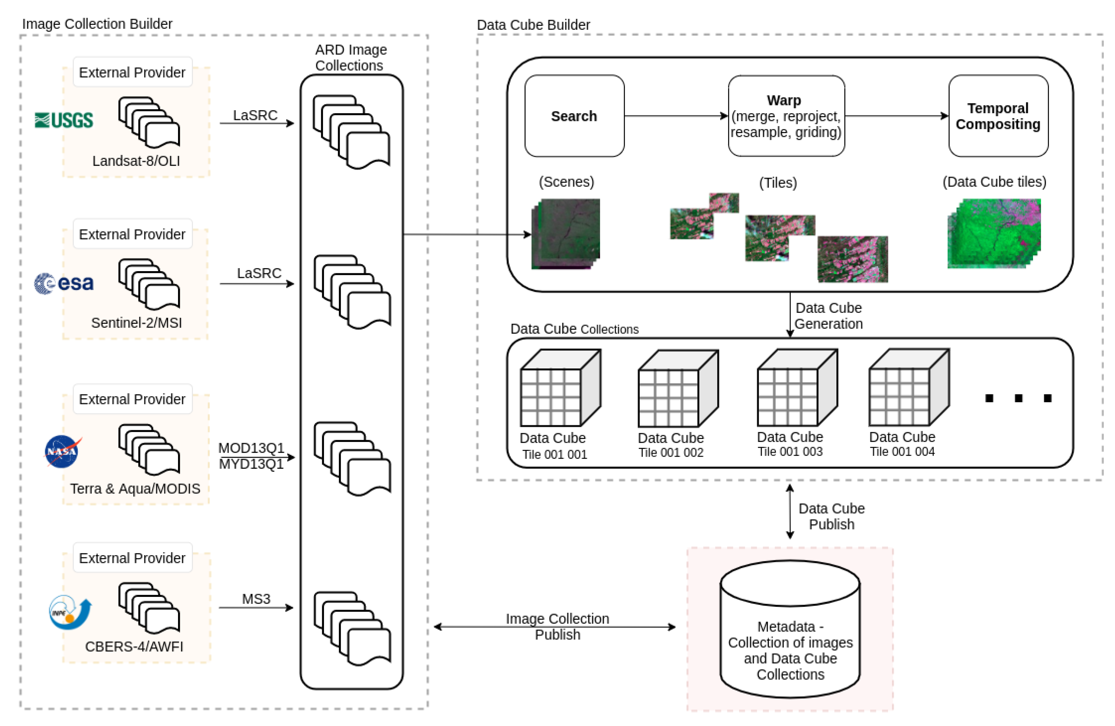
3.1. Data Acquisition and ARD Processing
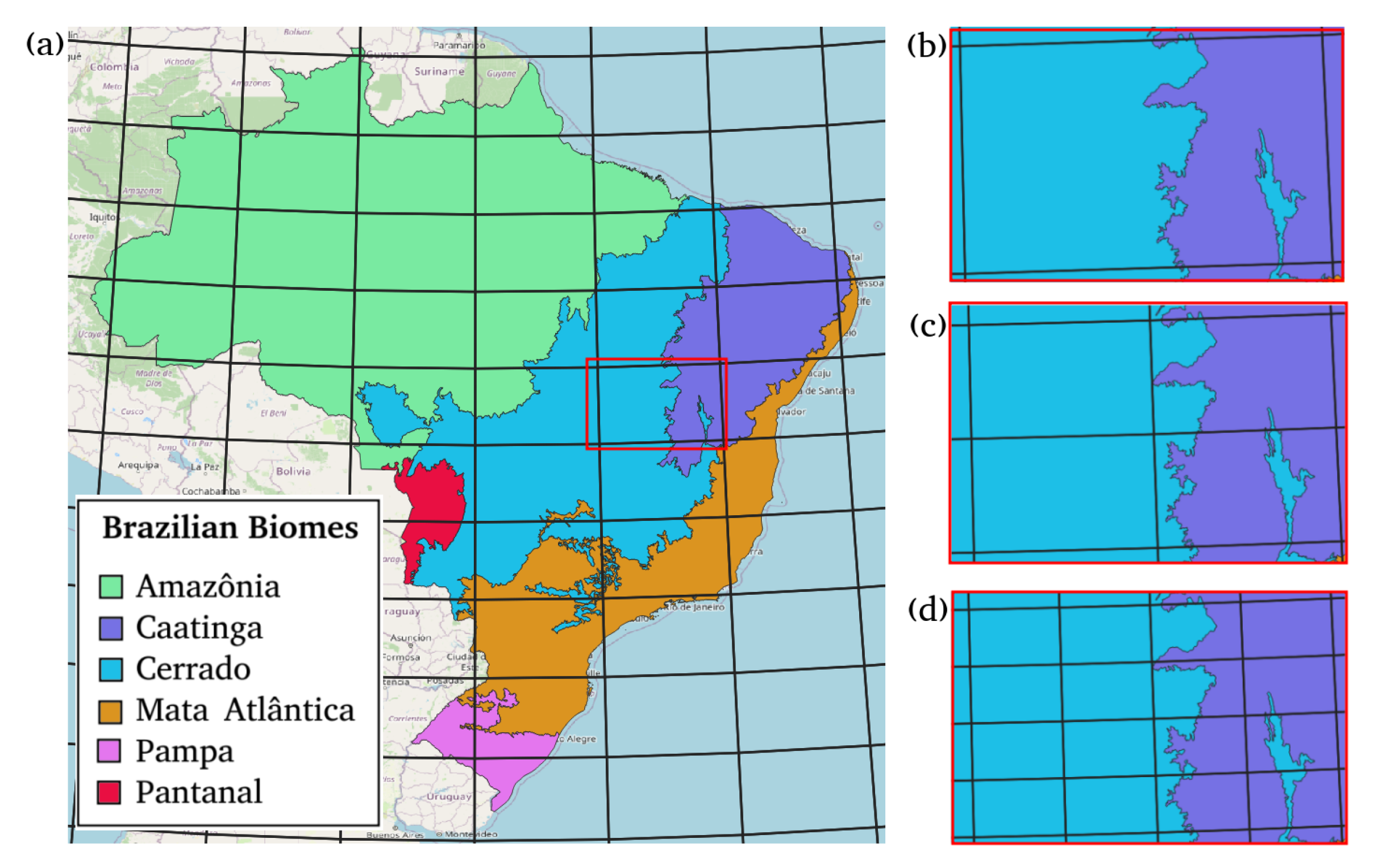
3.2. Tiling System
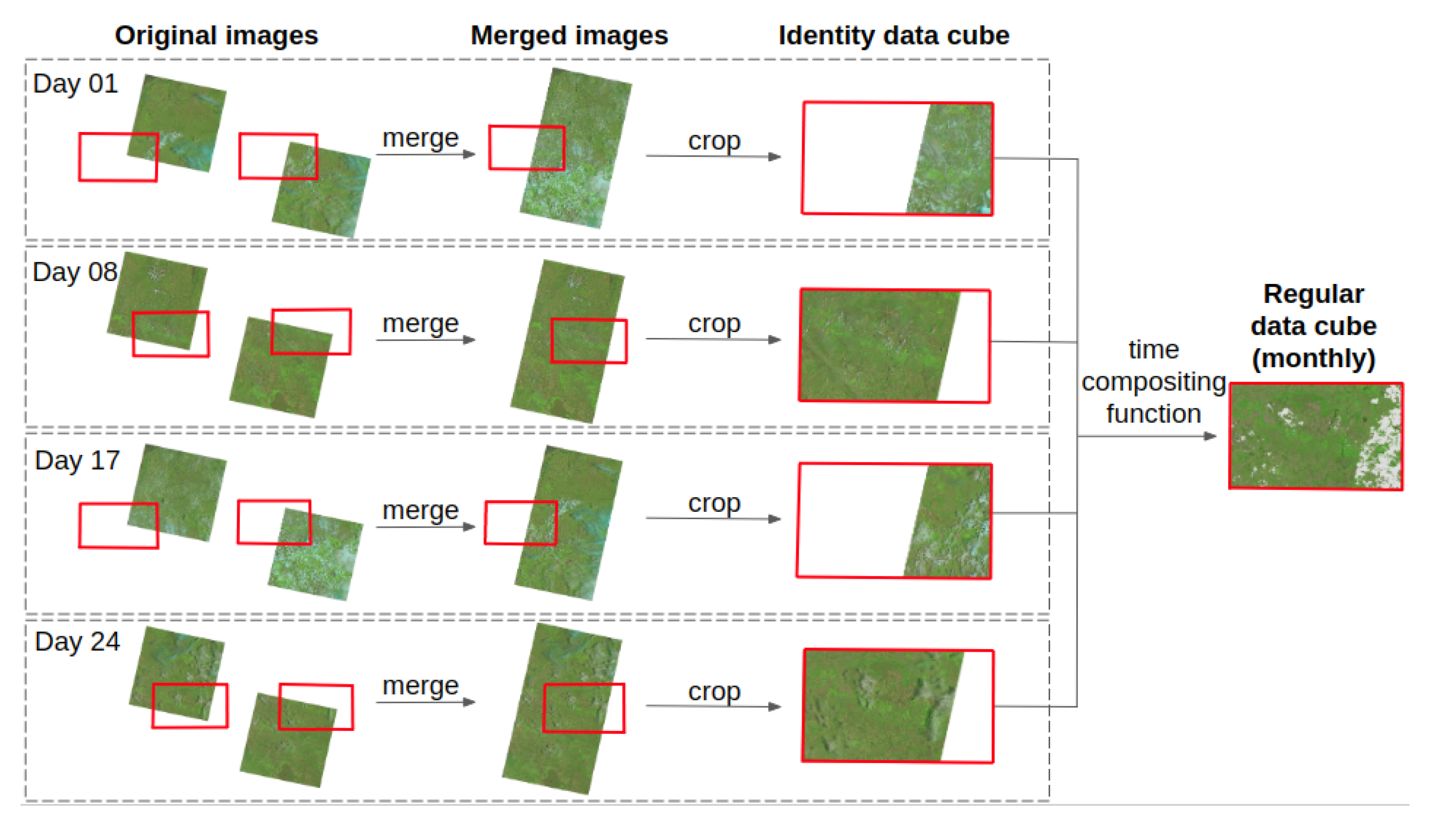
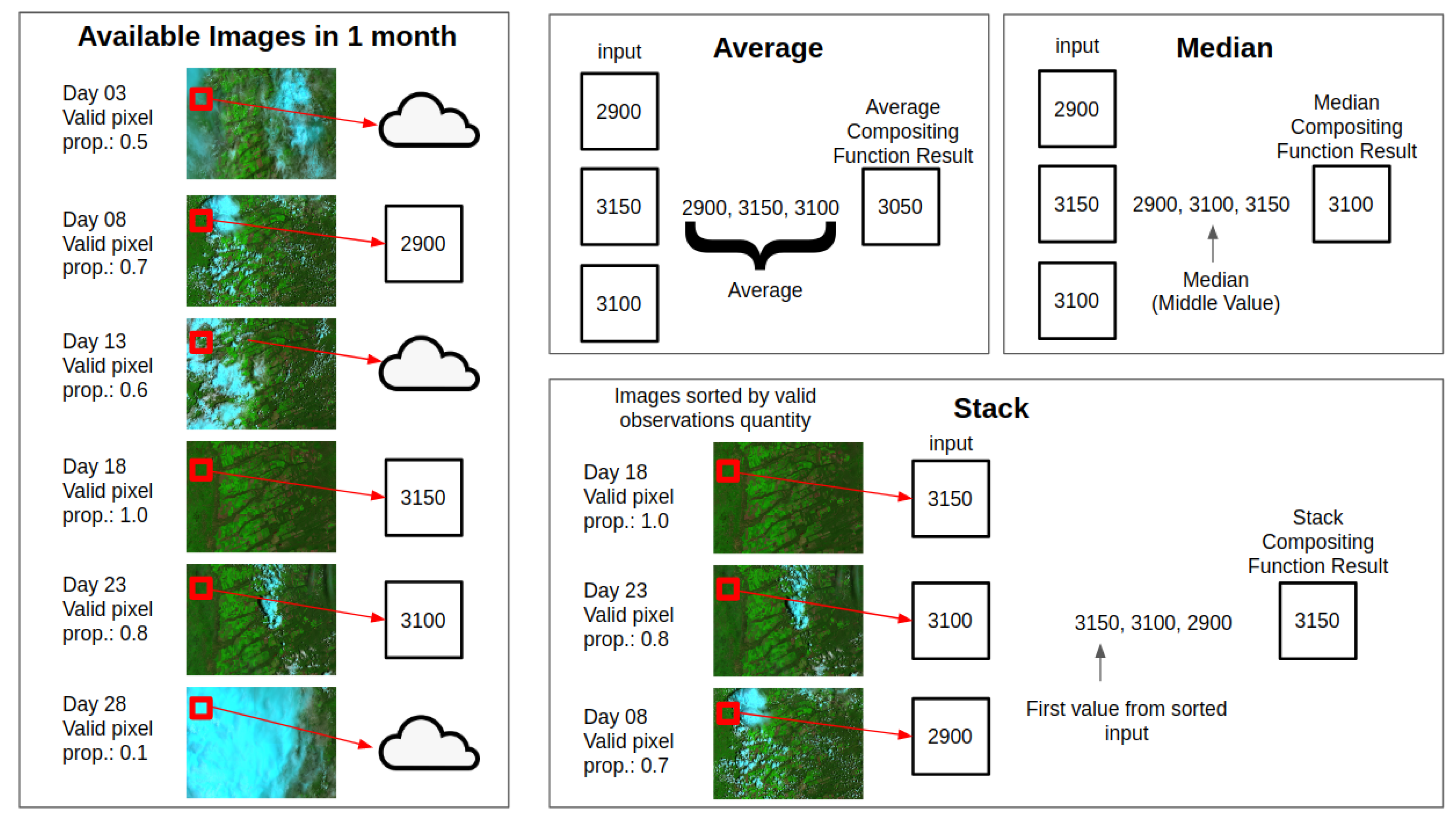
3.3. Data Cube Generation
3.4. Data Cube Validation and Metadata
4. Software and Data Products
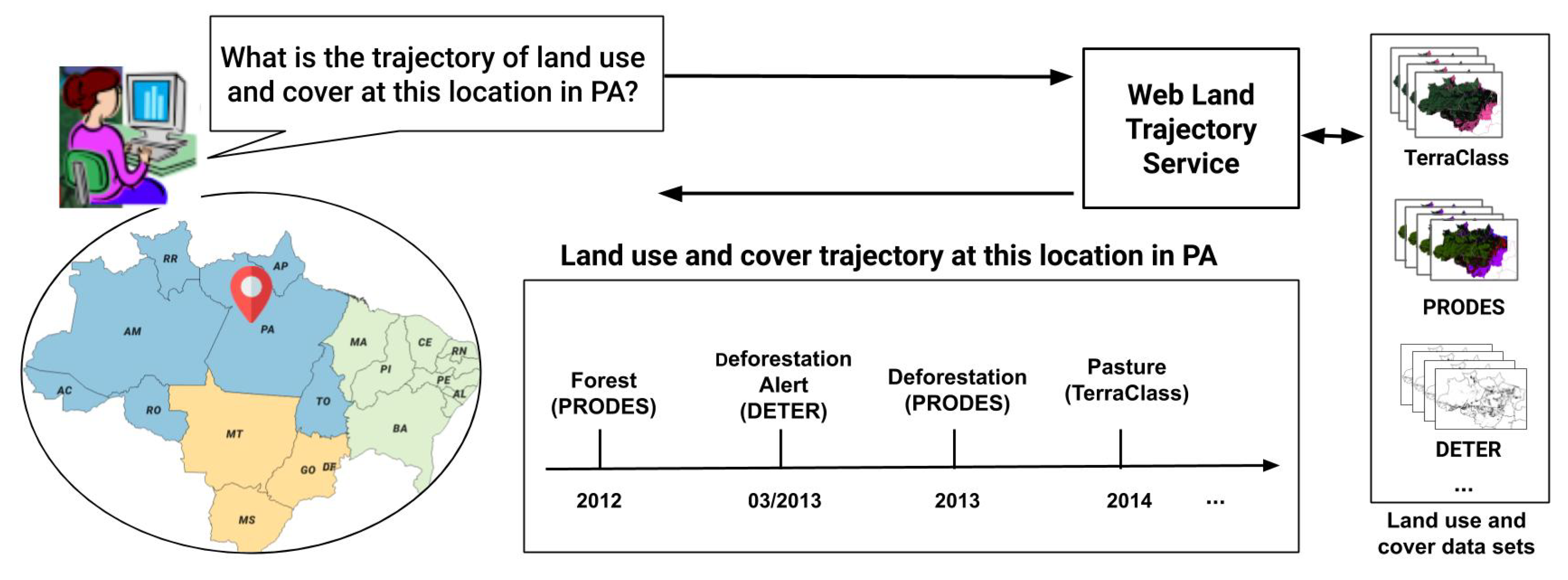
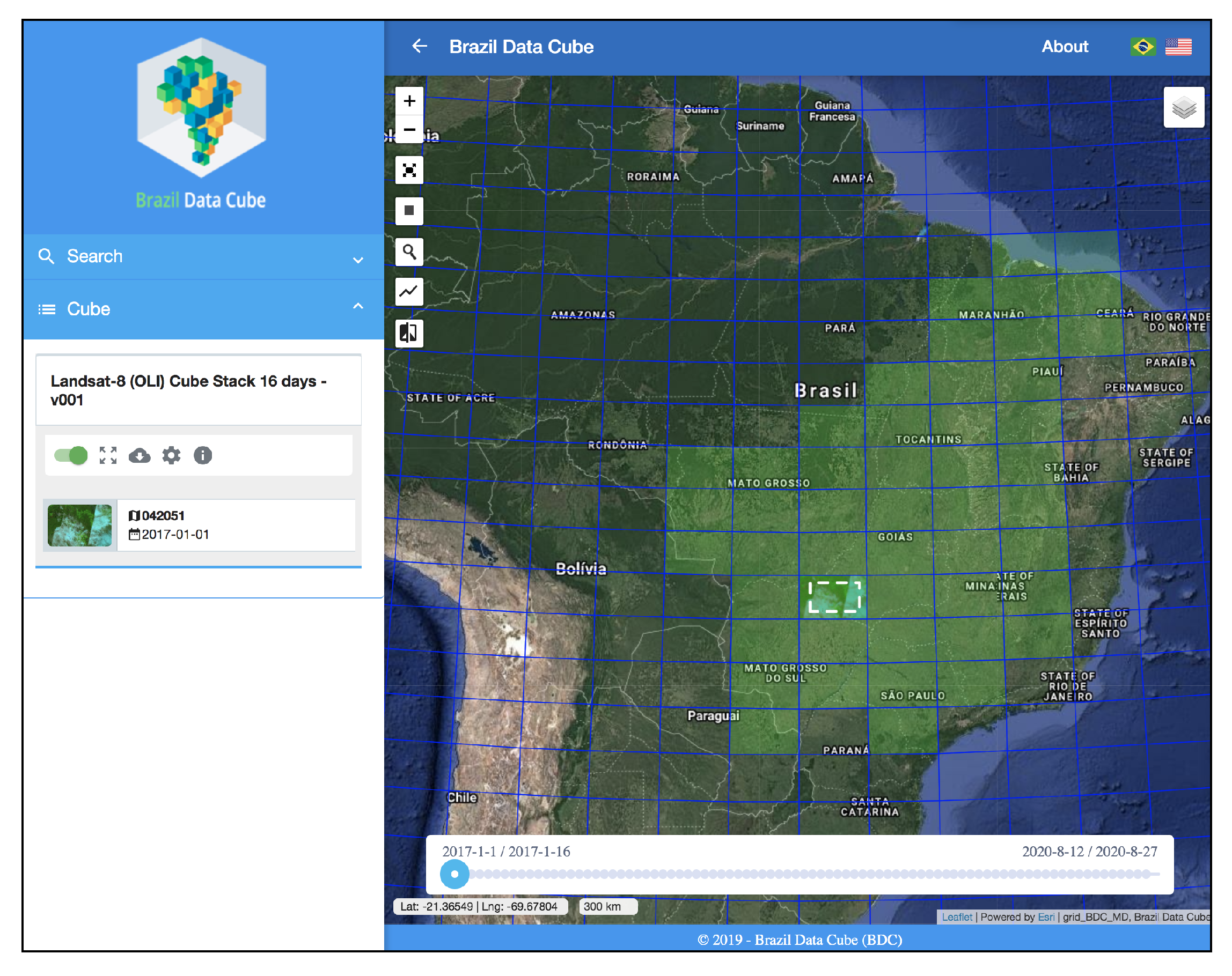
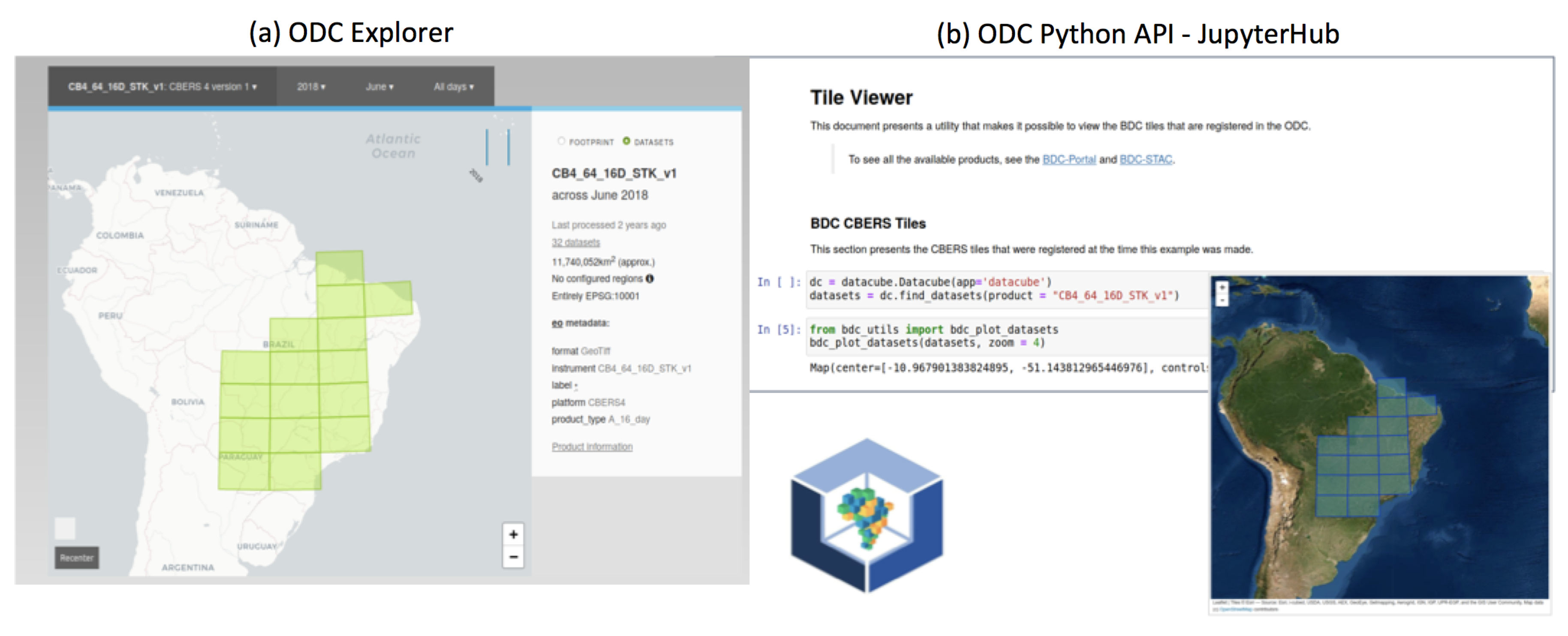
4.1. Web Services
4.2. Applications
5. Land Use and Cover Mapping from EO Data Cubes
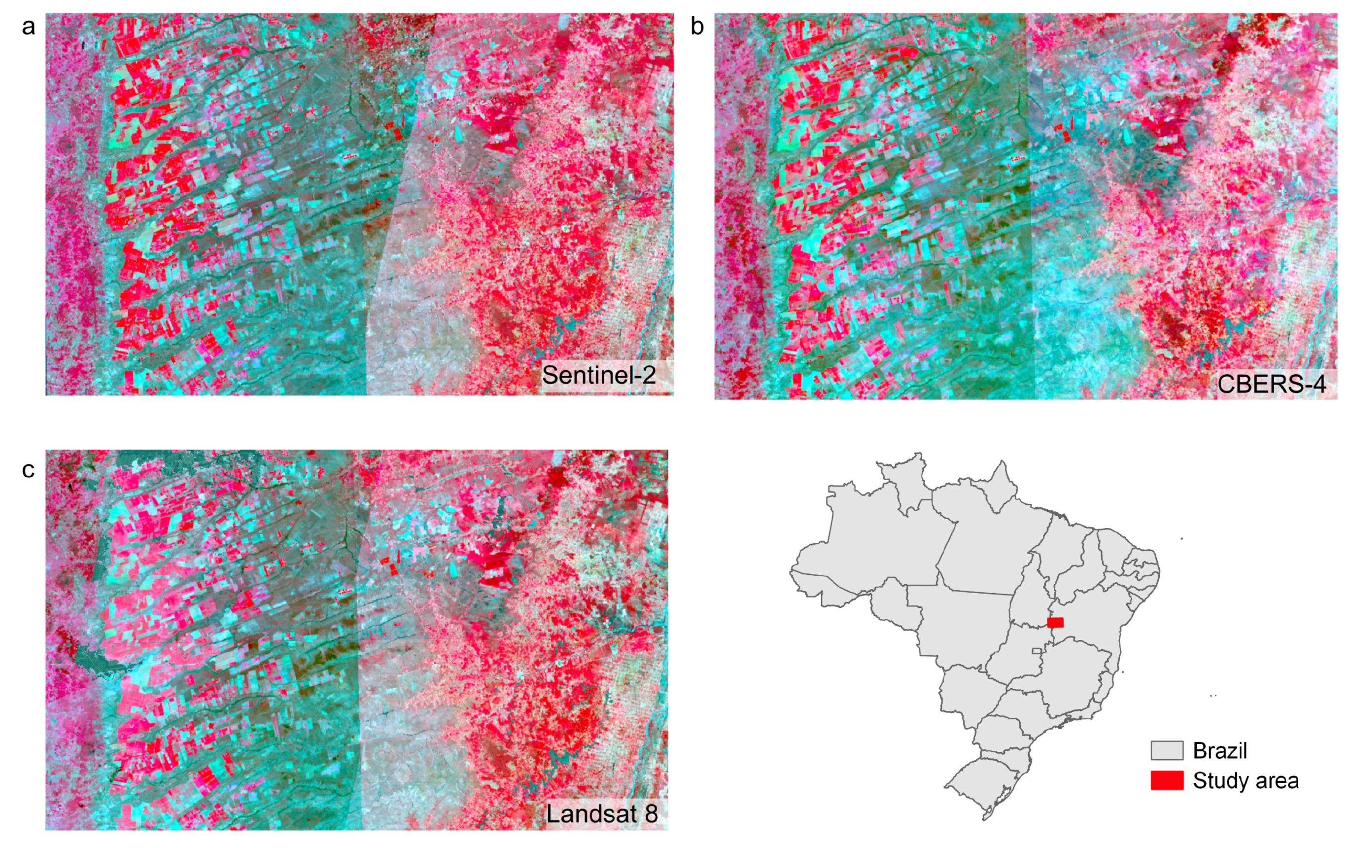
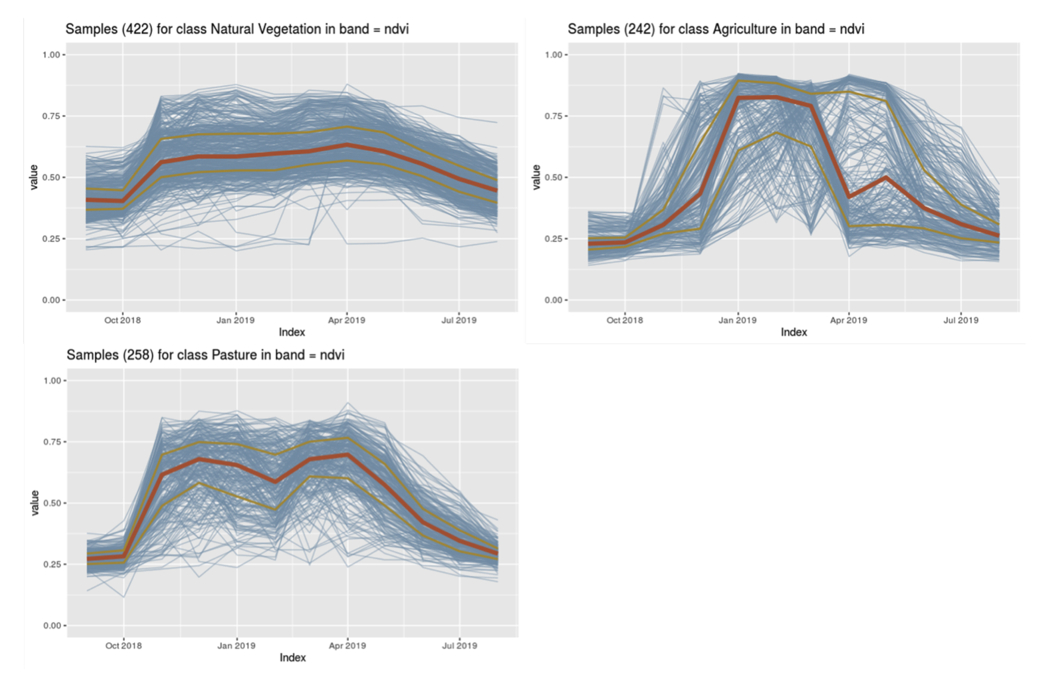
5.1. Study Area and Data
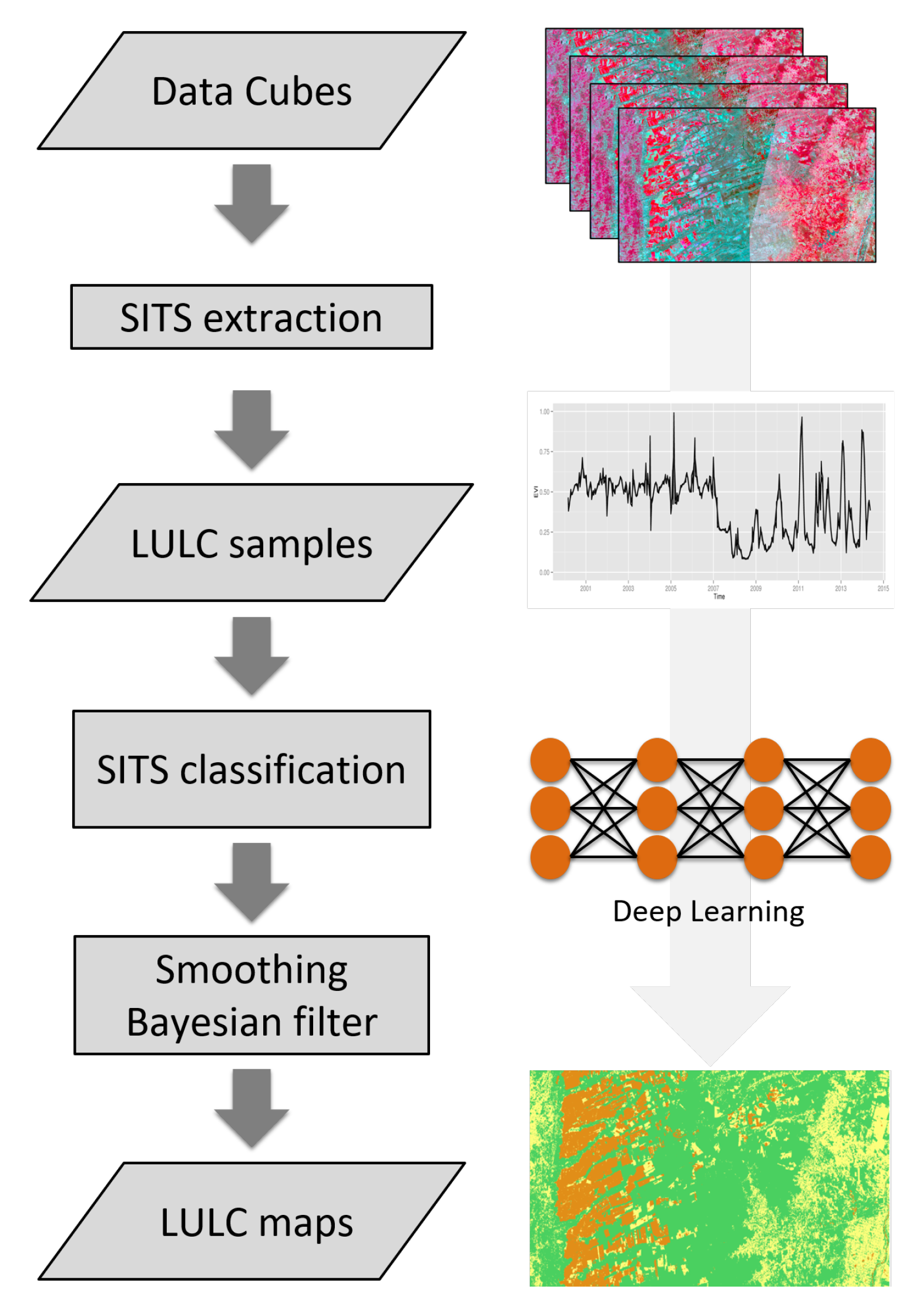
5.2. Classification Process
5.3. Results
6. Final Remarks and Future Directions
Author Contributions
Funding
Conflicts of Interest
References
- Foley, J.A.; DeFries, R.; Asner, G.P.; Barford, C.; Bonan, G.; Carpenter, S.R.; Chapin, F.S.; Coe, M.T.; Daily, G.C.; Gibbs, H.K.; et al. Global Consequences of Land Use. Science 2005, 309, 570–574. [Google Scholar] [CrossRef] [PubMed] [Green Version]
- Gomez, C.; White, J.C.; Wulder, M.A. Optical remotely sensed time series data for land cover classification: A review. J. Photogramm. Remote Sens. 2016, 116, 55–72. [Google Scholar] [CrossRef] [Green Version]
- Soille, P.; Burger, A.; Marchi, D.D.; Kempeneers, P.; Rodriguez, D.; Syrris, V.; Vasilev, V. A versatile data-intensive computing platform for information retrieval from big geospatial data. Future Gener. Comput. Syst. 2018, 81, 30–40. [Google Scholar] [CrossRef]
- Gomes, V.C.; Queiroz, G.R.; Ferreira, K.R. An Overview of Platforms for Big Earth Observation Data Management and Analysis. Remote Sens. 2020, 12, 1253. [Google Scholar] [CrossRef] [Green Version]
- Woodcock, C.E.; Loveland, T.R.; Herold, M.; Bauer, M.E. Transitioning from Change Detection to Monitoring with Remote Sensing: A Paradigm Shift. Remote Sens. Environ. 2020, 238, 111558. [Google Scholar] [CrossRef]
- Maus, V.; Câmara, G.; Cartaxo, R.; Sanchez, A.; Ramos, F.M.; de Queiroz, G.R. A Time-Weighted Dynamic Time Warping Method for Land-Use and Land-Cover Mapping. IEEE J. Sel. Top. Appl. Earth Obs. Remote Sens. 2016, 9, 3729–3739. [Google Scholar] [CrossRef]
- Belgiu, M.; Csillik, O. Sentinel-2 Cropland Mapping Using Pixel-Based and Object-Based Time-Weighted Dynamic Time Warping Analysis. Remote Sens. Environ. 2018, 204, 509–523. [Google Scholar] [CrossRef]
- Picoli, M.C.A.; Camara, G.; Sanches, I.; Simões, R.; Carvalho, A.; Maciel, A.; Coutinho, A.; Esquerdo, J.; Antunes, J.; Begotti, R.A.; et al. Big earth observation time series analysis for monitoring Brazilian agriculture. ISPRS J. Photogramm. Remote Sens. 2018, 145, 328–339. [Google Scholar] [CrossRef]
- Kong, Y.L.; Huang, Q.; Wang, C.; Chen, J.; Chen, J.; He, D. Long short-term memory neural networks for online disturbance detection in satellite image time series. Remote Sens. 2018, 10, 452. [Google Scholar] [CrossRef] [Green Version]
- Bendini, H.N.; Fonseca, L.M.G.; Schwieder, M.; Körting, T.S.; Rufin, P.; Sanches, I.D.A.; Leitão, P.J.; Hostert, P. Detailed agricultural land classification in the Brazilian cerrado based on phenological information from dense satellite image time series. Int. J. Appl. Earth Obs. Geoinf. 2019, 82, 101872. [Google Scholar] [CrossRef]
- Simoes, R.; Picoli, M.C.; Camara, G.; Maciel, A.; Santos, L.; Andrade, P.R.; Sánchez, A.; Ferreira, K.; Carvalho, A. Land use and cover maps for Mato Grosso State in Brazil from 2001 to 2017. Sci. Data 2020, 7, 1–10. [Google Scholar] [CrossRef] [PubMed] [Green Version]
- Lewis, A.; Oliver, S.; Lymburner, L.; Evans, B.; Wyborn, L.; Mueller, N.; Raevksi, G.; Hooke, J.; Woodcock, R.; Sixsmith, J.; et al. The Australian Geoscience Data Cube—Foundations and Lessons Learned. Remote Sens. Environ. 2017, 202, 276–292. [Google Scholar] [CrossRef]
- Siqueira, A.; Tadono, T.; Rosenqvist, A.; Lacey, J.; Lewis, A.; Thankappan, M.; Szantoi, Z.; Goryl, P.; Labahn, S.; Ross, J.; et al. CEOS Analysis Ready Data For Land–An Overview on the Current and Future Work. In Proceedings of the IGARSS 2019—2019 IEEE International Geoscience and Remote Sensing Symposium, Yokohama, Japan, 28 July–2 August 2019; IEEE: Piscataway, NJ, USA, 2019; pp. 5536–5537. [Google Scholar] [CrossRef]
- Giuliani, G.; Chatenoux, B.; De Bono, A.; Rodila, D.; Richard, J.P.; Allenbach, K.; Dao, H.; Peduzzi, P. Building an Earth Observations Data Cube: Lessons Learned from the Swiss Data Cube (SDC) on Generating Analysis Ready Data (ARD). Big Earth Data 2017, 1, 100–117. [Google Scholar] [CrossRef] [Green Version]
- Appel, M.; Pebesma, E. On-Demand Processing of Data Cubes from Satellite Image Collections with the Gdalcubes Library. Data 2019, 4, 92. [Google Scholar] [CrossRef] [Green Version]
- Asmaryan, S.; Muradyan, V.; Tepanosyan, G.; Hovsepyan, A.; Saghatelyan, A.; Astsatryan, H.; Grigoryan, H.; Abrahamyan, R.; Guigoz, Y.; Giuliani, G. Paving the Way towards an Armenian Data Cube. Data 2019, 4, 117. [Google Scholar] [CrossRef] [Green Version]
- Maso, J.; Zabala, A.; Serral, I.; Pons, X. A Portal Offering Standard Visualization and Analysis on top of an Open Data Cube for Sub-National Regions: The Catalan Data Cube Example. Data 2019, 4, 96. [Google Scholar] [CrossRef] [Green Version]
- Killough, B. The Impact of Analysis Ready Data in the Africa Regional Data Cube. In Proceedings of the IGARSS 2019—2019 IEEE International Geoscience and Remote Sensing Symposium, Yokohama, Japan, 28 July–2 August 2019; IEEE: Piscataway, NJ, USA, 2019; pp. 5646–5649. [Google Scholar] [CrossRef]
- Camara, G.; Assis, L.F.; Ribeiro, G.; Ferreira, K.R.; Llapa, E.; Vinhas, L. Big Earth Observation Data Analytics: Matching Requirements to System Architectures. In Proceedings of the 5th ACM SIGSPATIAL International Workshop on Analytics for Big Geospatial Data, BigSpatial ’16, San Francisco, CA, USA, 31 October 2016; Association for Computing Machinery: New York, NY, USA, 2016; pp. 1–6. [Google Scholar] [CrossRef]
- Gorelick, N.; Hancher, M.; Dixon, M.; Ilyushchenko, S.; Thau, D.; Moore, R. Google Earth Engine: Planetary-scale geospatial analysis for everyone. Remote Sens. Environ. 2017. [Google Scholar] [CrossRef]
- Giuliani, G.; Camara, G.; Killough, B.; Minchin, S. Earth Observation Open Science: Enhancing Reproducible Science Using Data Cubes. Data 2019, 4, 147. [Google Scholar] [CrossRef] [Green Version]
- Ponzoni, F.J.; Junior, J.Z.; Lamparelli, R.A. In-flight absolute calibration of the CBERS-2 CCD sensor data. Acad. Bras. CiÊNcias 2008, 80, 373–380. [Google Scholar] [CrossRef] [Green Version]
- Diniz, C.G.; Souza, A.A.; Santos, D.C.; Dias, M.C.; Luz, N.C.; Moraes, D.R.V.; Maia, J.S.; Gomes, A.R.; Narvaes, I.; Valeriano, D.M.; et al. DETER-B: The New Amazon Near Real-Time Deforestation Detection System. IEEE J. Sel. Top. Appl. Earth Obs. Remote Sens. 2015, 8, 3619–3628. [Google Scholar] [CrossRef]
- INPE. PRODES Project: Brazilian Amazon Forest Monitoring by Satellite. Available online: http://www.obt.inpe.br/OBT/assuntos/programas/amazonia/prodes (accessed on 28 December 2019).
- FG Assis, L.F.; Ferreira, K.R.; Vinhas, L.; Maurano, L.; Almeida, C.; Carvalho, A.; Rodrigues, J.; Maciel, A.; Camargo, C. TerraBrasilis: A Spatial Data Analytics Infrastructure for Large-Scale Thematic Mapping. ISPRS Int. J. Geo-Inf. 2019, 8, 513. [Google Scholar] [CrossRef] [Green Version]
- Almeida, C.A.D.; Coutinho, A.C.; Esquerdo, J.C.D.M.; Adami, M.; Venturieri, A.; Diniz, C.G.; Dessay, N.; Durieux, L.; Gomes, A.R. High spatial resolution land use and land cover mapping of the Brazilian Legal Amazon in 2008 using Landsat-5/TM and MODIS data. Acta Amaz. 2016, 46, 291–302. [Google Scholar] [CrossRef]
- Kintisch, E. Improved monitoring of rainforests helps pierce haze of deforestation. Science 2007, 316, 536–537. [Google Scholar] [CrossRef] [PubMed]
- Maus, V.; Câmara, G.; Appel, M.; Pebesma, E. dtwSat: Time-Weighted Dynamic Time Warping for Satellite Image Time Series Analysis in R. J. Stat. Softw. Artic. 2019, 88, 1–31. [Google Scholar] [CrossRef] [Green Version]
- Xi, W.; Du, S.; Wang, Y.C.; Zhang, X. A Spatiotemporal Cube Model for Analyzing Satellite Image Time Series: Application to Land-Cover Mapping and Change Detection. Remote Sens. Environ. 2019. [Google Scholar] [CrossRef]
- Santos, L.; Ferreira, K.R.; Picoli, M.; Camara, G. Self-Organizing Maps in Earth Observation Data Cubes Analysis. In Advances in Self-Organizing Maps, Learning Vector Quantization, Clustering and Data Visualization; Vellido, A., Gibert, K., Angulo, C., Martín Guerrero, J.D., Eds.; Springer International Publishing: Cham, Switzerland, 2020; pp. 70–79. [Google Scholar]
- Lu, M.; Pebesma, E.; Sanchez, A.; Verbesselt, J. Spatio-temporal change detection from multidimensional arrays: Detecting deforestation from MODIS time series. ISPRS J. Photogramm. Remote Sens. 2016, 117, 227–236. [Google Scholar] [CrossRef]
- Camara, G.; Simoes, R.; Andrade, P.R.; Maus, V.; Sánchez, A.; de Assis, L.F.F.G.; Santos, L.A.; Ywata, A.C.; Maciel, A.M.; Vinhas, L.; et al. e-sensing/sits: Version 1.12.5; Zenodo: Geneva, Switzerland, 2018. [Google Scholar] [CrossRef]
- Vinhas, L.; de Queiroz, G.R.; Ferreira, K.R.; Camara, G. Web services for big earth observation data. Rev. Bras. Cartogr. 2017, 69, 5. [Google Scholar]
- Müller, M.; Bernard, L.; Brauner, J. Moving code in spatial data infrastructures - Web service based deployment of geoprocessing algorithms. Trans. GIS 2010, 14, 101–118. [Google Scholar] [CrossRef]
- Amazon Web Services. Open Data on AWS. Available online: https://aws.amazon.com/opendata/ (accessed on 26 March 2020).
- Ferreira, K.R.; Queiroz, G.R.; Camara, G.; Souza, R.C.M.; Vinhas, L.; Marujo, R.F.B.; Simoes, R.E.O.; Noronha, C.A.F.; Costa, R.W.; Arcanjo, J.S.; et al. Using Remote Sensing Images and Cloud Services on AWS to Improve Land Use and Cover Monitoring. In Proceedings of the 2020 IEEE Latin American GRSS ISPRS Remote Sensing Conference (LAGIRS), Santiago, Chile, 22–26 March 2020; pp. 558–562. [Google Scholar]
- Vermote, E.; Justice, C.; Claverie, M.; Franch, B. Preliminary analysis of the performance of the Landsat 8/OLI land surface reflectance product. Remote Sens. Environ. 2016, 185, 46–56. [Google Scholar] [CrossRef]
- Da Silva, M.A.O.; de Andrade, A.C. Geração de imagens de reflectância de um ponto de vista geométrico. Rev. Bras. Geomat. 2013, 1, 23. [Google Scholar] [CrossRef]
- Qiu, S.; Zhu, Z.; He, B. Fmask 4.0: Improved cloud and cloud shadow detection in Landsats 4–8 and Sentinel-2 imagery. Remote Sens. Environ. 2019, 231, 111205. [Google Scholar] [CrossRef]
- Sanchez, A.H.; Picoli, M.C.A.; Camara, G.; Andrade, P.R.; Chaves, M.E.D.; Lechler, S.; Soares, A.R.; Marujo, R.F.B.; Simões, R.E.O.; Ferreira, K.R.; et al. Comparison of Cloud Cover Detection Algorithms on Sentinel–2 Images of the Amazon Tropical Forest. Remote Sens. 2020, 12, 1284. [Google Scholar] [CrossRef] [Green Version]
- Sattler, K.U. Data Quality Dimensions. Encycl. Database Syst. 2016, 1–5. [Google Scholar] [CrossRef]
- STAC. SpatioTemporal Asset Catalogs. Available online: https://stacspec.org/ (accessed on 2 October 2020).
- OGC. OGC Standards and Supporting Documents. Available online: http://www.opengeospatial.org/standards/ (accessed on 1 October 2020).
- De Oliveira, S.N.; de Carvalho Júnior, O.A.; Gomes, R.A.T.; Guimarães, R.F.; McManus, C.M. Landscape-fragmentation change due to recent agricultural expansion in the Brazilian Savanna, Western Bahia, Brazil. Reg. Environ. Chang. 2017, 17, 411–423. [Google Scholar] [CrossRef]
- Hastie, T.; Tibshirani, R. The Elements of Statistical Learning. Data Mining, Inference, and Prediction; Springer: New York, NY, USA, 2009. [Google Scholar]
- Olofsson, P.; Foody, G.M.; Herold, M.; Stehman, S.V.; Woodcock, C.E.; Wulder, M.A. Good Practices for Estimating Area and Assessing Accuracy of Land Change. Remote Sens. Environ. 2014, 148, 42–57. [Google Scholar] [CrossRef]
- Chaves, M.E.D.; Picoli, M.C.A.; Sanches, I.D. Recent Applications of Landsat 8/OLI and Sentinel-2/MSI for Land Use and Land Cover Mapping: A Systematic Review. Remote Sens. 2020, 12, 3062. [Google Scholar] [CrossRef]
- Claverie, M.; Masek, J.G.; Ju, J.; Dungan, J.L. Harmonized Landsat-8 Sentinel-2 (HLS) Product User’s Guide: Product Version 1.3; National Aeronautics and Space Administration (NASA): Washington, DC, USA, 2017.
- Roy, D.P.; Zhang, H.K.; Ju, J.; Gomez-Dans, J.L.; Lewis, P.E.; Schaaf, C.B.; Sun, Q.; Li, J.; Huang, H.; Kovalskyy, V. A general method to normalize Landsat reflectance data to nadir BRDF adjusted reflectance. Remote Sens. Environ. 2016, 176, 255–271. [Google Scholar] [CrossRef] [Green Version]
- Roy, D.P.; Li, J.; Zhang, H.K.; Yan, L.; Huang, H.; Li, Z. Examination of Sentinel-2A multi-spectral instrument (MSI) reflectance anisotropy and the suitability of a general method to normalize MSI reflectance to nadir BRDF adjusted reflectance. Remote Sens. Environ. 2017, 199, 25–38. [Google Scholar] [CrossRef]
- Claverie, M.; Ju, J.; Masek, J.G.; Dungan, J.L.; Vermote, E.F.; Roger, J.C.; Skakun, S.V.; Justice, C. The Harmonized Landsat and Sentinel-2 Surface Reflectance Data Set. Remote Sens. Environ. 2018, 219, 145–161. [Google Scholar] [CrossRef]
- Franch, B.; Vermote, E.; Skakun, S.; Roger, J.c.; Masek, J.; Ju, J.; Villaescusa-nadal, J.L.; Santamaria-artigas, A. A Method for Landsat and Sentinel 2 (HLS) BRDF Normalization. Remote Sens. 2019, 2, 632. [Google Scholar] [CrossRef] [Green Version]
- Steinhausen, M.J.; Wagner, P.D.; Narasimhan, B.; Waske, B. Combining Sentinel-1 and Sentinel-2 data for improved land use and land cover mapping of monsoon regions. Int. J. Appl. Earth Obs. Geoinf. 2018, 73, 595–604. [Google Scholar] [CrossRef]
- Nicolau, A.P.; Flores-Anderson, A.; Griffin, R.; Herndon, K.; Meyer, F.J. Assessing SAR C-band data to effectively distinguish modified land uses in a heavily disturbed Amazon forest. Int. J. Appl. Earth Obs. Geoinf. 2021, 94, 102214. [Google Scholar] [CrossRef]


| Grid | Collection | Extension | Image Size |
|---|---|---|---|
| BDC_LG | CBERS-4 AWFI (64 m) | km | 10,504 6865 pixels |
| BDC_MD | Landsat-8 OLI (30 m) | km | 11,204 7324 pixels |
| BDC_SM | Sentinel-2 MSI (10 m) | km | 16,806 × 10,986 pixels |
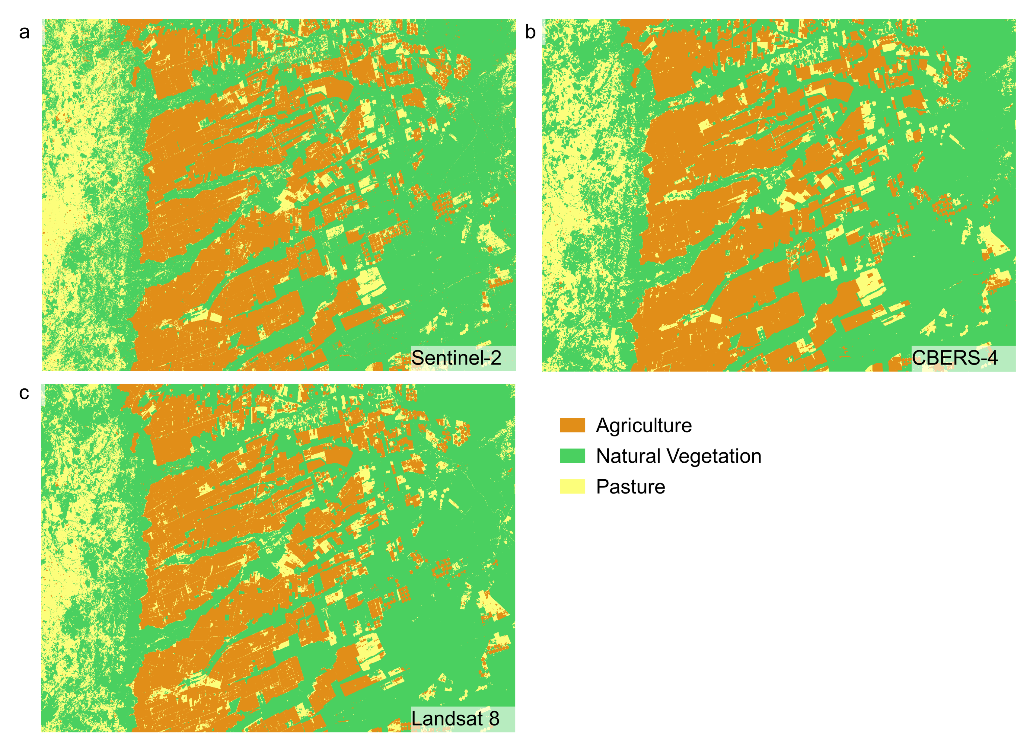
| Accuracy | CBERS-4 | Sentinel-2 | Landsat 8 |
|---|---|---|---|
| PA Anthropic | 0.81 | 0.90 | 0.94 |
| PA Nat. Veg. | 0.67 | 0.84 | 0.85 |
| UA Anthropic | 0.71 | 0.85 | 0.86 |
| UA Nat. Veg. | 0.78 | 0.90 | 0.94 |
| OA | 0.74 | 0.87 | 0.90 |
Publisher’s Note: MDPI stays neutral with regard to jurisdictional claims in published maps and institutional affiliations. |
© 2020 by the authors. Licensee MDPI, Basel, Switzerland. This article is an open access article distributed under the terms and conditions of the Creative Commons Attribution (CC BY) license (http://creativecommons.org/licenses/by/4.0/).
Share and Cite
Ferreira, K.R.; Queiroz, G.R.; Vinhas, L.; Marujo, R.F.B.; Simoes, R.E.O.; Picoli, M.C.A.; Camara, G.; Cartaxo, R.; Gomes, V.C.F.; Santos, L.A.; et al. Earth Observation Data Cubes for Brazil: Requirements, Methodology and Products. Remote Sens. 2020, 12, 4033. https://0-doi-org.brum.beds.ac.uk/10.3390/rs12244033
Ferreira KR, Queiroz GR, Vinhas L, Marujo RFB, Simoes REO, Picoli MCA, Camara G, Cartaxo R, Gomes VCF, Santos LA, et al. Earth Observation Data Cubes for Brazil: Requirements, Methodology and Products. Remote Sensing. 2020; 12(24):4033. https://0-doi-org.brum.beds.ac.uk/10.3390/rs12244033
Chicago/Turabian StyleFerreira, Karine R., Gilberto R. Queiroz, Lubia Vinhas, Rennan F. B. Marujo, Rolf E. O. Simoes, Michelle C. A. Picoli, Gilberto Camara, Ricardo Cartaxo, Vitor C. F. Gomes, Lorena A. Santos, and et al. 2020. "Earth Observation Data Cubes for Brazil: Requirements, Methodology and Products" Remote Sensing 12, no. 24: 4033. https://0-doi-org.brum.beds.ac.uk/10.3390/rs12244033