Article

Design and Development of a Smart Variable Rate Sprayer Using Deep Learning

1
Faculty of Sustainable Design Engineering, University of Prince Edward Island, Charlottetown, PE C1A4P3, Canada
2
Citrus Research and Education Center, University of Florida, Lake Alfred, FL 33850, USA
3
Agriculture and Agri-Food Canada, Research and Development Centre, Charlottetown, PE C1A4N6, Canada
4
Engineering Department, Faculty of Agriculture, Dalhousie University, Truro, NS B2N5E3, Canada
5
Department of Chemical and Biological Engineering, University of Saskatchewan, Saskatoon, SK S7N5A9, Canada
*
Author to whom correspondence should be addressed.
Remote Sens. 2020, 12(24), 4091; https://0-doi-org.brum.beds.ac.uk/10.3390/rs12244091
Submission received: 10 November 2020 / Revised: 14 December 2020 / Accepted: 14 December 2020 / Published: 15 December 2020

Abstract

:
The uniform application (UA) of agrochemicals results in the over-application of harmful chemicals, increases crop input costs, and deteriorates the environment when compared with variable rate application (VA). A smart variable rate sprayer (SVRS) was designed, developed, and tested using deep learning (DL) for VA application of agrochemicals. Real-time testing of the SVRS took place for detecting and spraying and/or skipping lambsquarters weed and early blight infected and healthy potato plants. About 24,000 images were collected from potato fields in Prince Edward Island and New Brunswick under varying sunny, cloudy, and partly cloudy conditions and processed/trained using YOLOv3 and tiny-YOLOv3 models. Due to faster performance, the tiny-YOLOv3 was chosen to deploy in SVRS. A laboratory experiment was designed under factorial arrangements, where the two spraying techniques (UA and VA) and the three weather conditions (cloudy, partly cloudy, and sunny) were the two independent variables with spray volume consumption as a response variable. The experimental treatments had six repetitions in a 2 × 3 factorial design. Results of the two-way ANOVA showed a significant effect of spraying application techniques on volume consumption of spraying liquid (p-value < 0.05). There was no significant effect of weather conditions and interactions between the two independent variables on volume consumption during weeds and simulated diseased plant detection experiments (p-value > 0.05). The SVRS was able to save 42 and 43% spraying liquid during weeds and simulated diseased plant detection experiments, respectively. Water sensitive papers’ analysis showed the applicability of SVRS for VA with >40% savings of spraying liquid by SVRS when compared with UA. Field applications of this technique would reduce the crop input costs and the environmental risks in conditions (weed and disease) like experimental testing.

Graphical Abstract

1. Introduction

Site-specific variable rate application (VA) of herbicides is preferred over uniform application (UA) to kill weeds and/or disease infections present in patches in agricultural fields. Uniform application of agrochemicals causes over-application of harmful chemicals, increases crop input costs, deteriorates the environment [1,2,3], risks human health [4], and results in low application efficiency of sprayers [5]. A smart variable rate sprayer (SVRS) uses available electronics and automation in agricultural machinery [6] for optimization of agrochemical applications through a sensor-based control system that helps apply agrochemicals as and when required [7].
There are different spaying methods for agrochemical field applications, including broadcasting and band applications. The former is inefficient as it uniformly applies chemicals in agricultural fields without considering the variable conditions of the field. By using this technique, around 60–70% of spraying chemicals are wasted [8]. Variable-rate technology, on the other hand, saves the spraying chemicals and reduces environmental degradation. Almost 40% of herbicides can be saved by considering the patches of weeds and/or disease infections in the field during the spraying operation. For bushes and tree crops, up to 75% of pesticides can be saved by variably applying the chemicals according to the canopy structure of trees [9].
The use of artificial intelligence (AI) can significantly improve the efficiency of sprayers [10]. The AI uses data-driven modeling techniques by taking the processed and labeled images of the targets as input for the development of a machine vision system. Target plants are detected on the basis of morphology and texture of plants [11].
Real-time detections of targets depend upon several factors, including the quality and quantity of images, design of deep convolutional neural networks (DCNN), available memory resources such as graphical processing units (GPU), and the related hardware. Qiongyan et al. [12] used convolutional neural networks (CNNs) to identify wheat spikes with 86.6% detection accuracy for the quantification of phenotypic changes that arise genetically or due to environmental variations. Deep learning (DL) models were used for counting wheat spikes and spikelet with 95.9 and 99.7% accuracies, respectively [13]. Yang and Sun [14] reported that DCNNs are supportive of agricultural applications. They used DCNN models to classify weeds with >95% accuracy. Milioto et al. [15] reported achieving high classification accuracy (99%) using CNNs for sugar beets and weeds distinction.
The DCNN models can also be applied for disease recognition in the plants. Wheat disease was identified by using DCNN models with 95% accuracy [16]. In addition, the trained models were used as a smartphone application for real-time recognition of disease-infected plants in crops. Liakos et al. [17] detected yellow-rust-infected plants of wheat with 99.4% accuracy in wheat crops using CNNs. Object detection models may be used for detection, as well as real-time applications of agrochemicals, with high accuracy [18].
A rapid surge can be observed in the literature about the applications of object detection models, including autonomous vehicles, agriculture robots, and other machine vision tasks. Among several object detection CNNs, YOLO, and single-shot detectors are comparatively faster and more accurate models in object recognition [19]. The YOLOv3 was used in small aircraft detection, and it performed well concerning accuracy as well as detection speed [20]. Thai traffic signs were detected and recognized using CNNs with 93% average precision [21]. The Tiny-YOLOv3 was designed by simplifying the YOLOv3 algorithm and reducing the depth of convolutional layers, which significantly improved the inference speed and is also ideal for running on personal computers [22].
Many researchers have developed vision-based spot-applicators for weed detection that operate in real-time using a variety of remote sensing devices [23]. Vision-based algorithms were applied to develop variable rate systems for target detection using Raspberry Pi and OpenCV in drone systems by Pathak et al. [24]. Machine-learning-based systems gave good accuracy [25] in real-time target detection [26]. Partel et al. [27] developed and evaluated a low-cost smart sprayer for agrochemical spraying on weeds at a lab scale, utilizing YOLO models, and reported 40 to 90% accuracy using different Nvidia GPUs. The automated variable-rate sprayers were also developed for disease and pest control [28,29] and for the detection of weeds [30] using machine learning (ML) techniques. Möller [31] concluded that computer vision technologies for VA in agricultural fields could reduce the inputs and lower the operator’s stress levels. It can locate weed spots in real-time and spray the chemical only on proper locations. They [31] obtained a significant reduction in the total amount of applied volume (58%) using a VA prototype in comparison with a conventional UA during lab experimentation.
It has been reported in the literature that YOLO is suitable for real-time weed and disease detection. Therefore, an object detection DCNN tiny-YOLOv3 was selected for detection of a potato weed (lambsquarters) and simulated disease (early blight) infected plants at a laboratory scale. Furthermore, a trained tiny-YOLOv3 model was deployed and tested on a newly designed and developed SVRS for VA and site-specific agrochemical applications in potato crops.

2. Materials and Methods

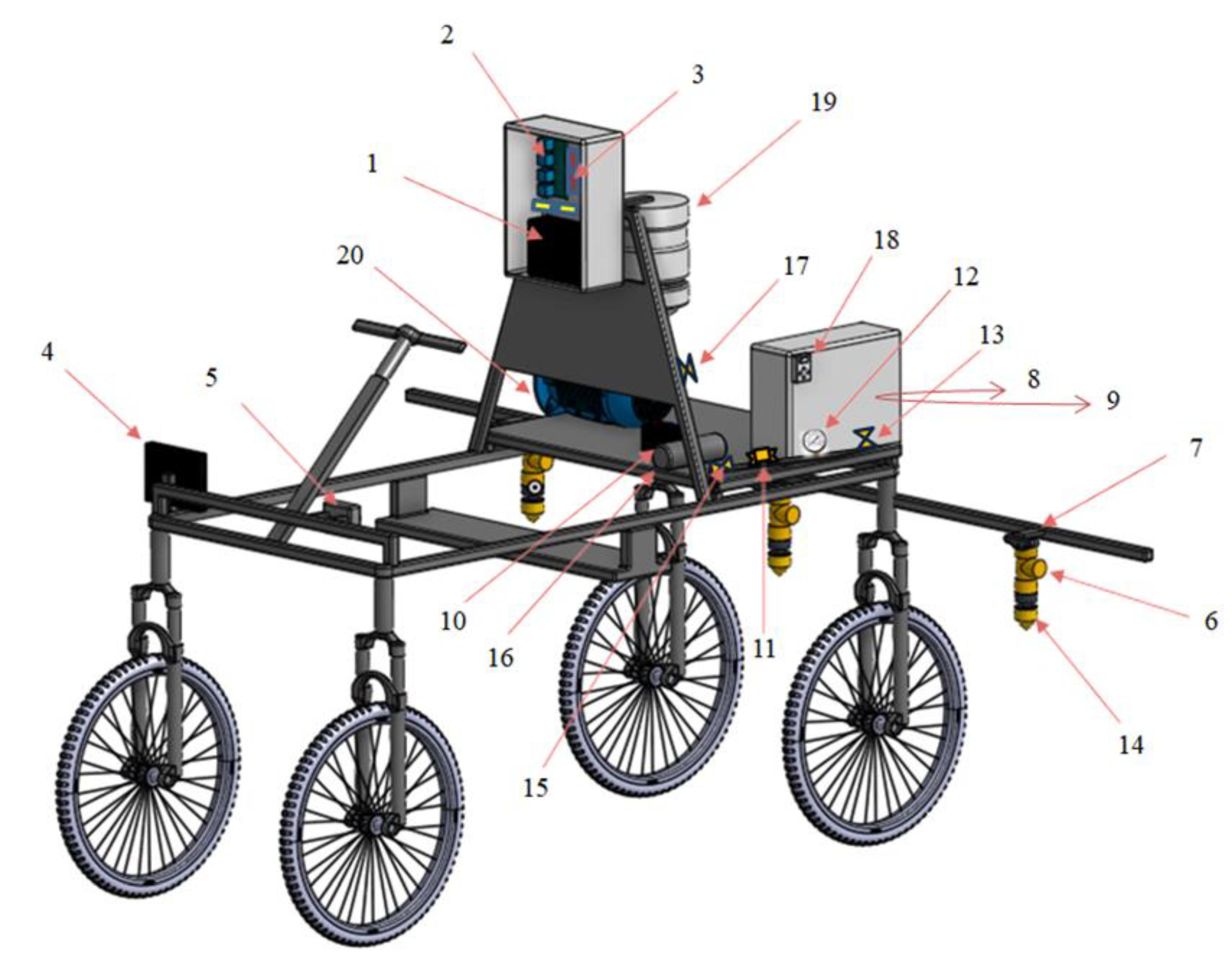
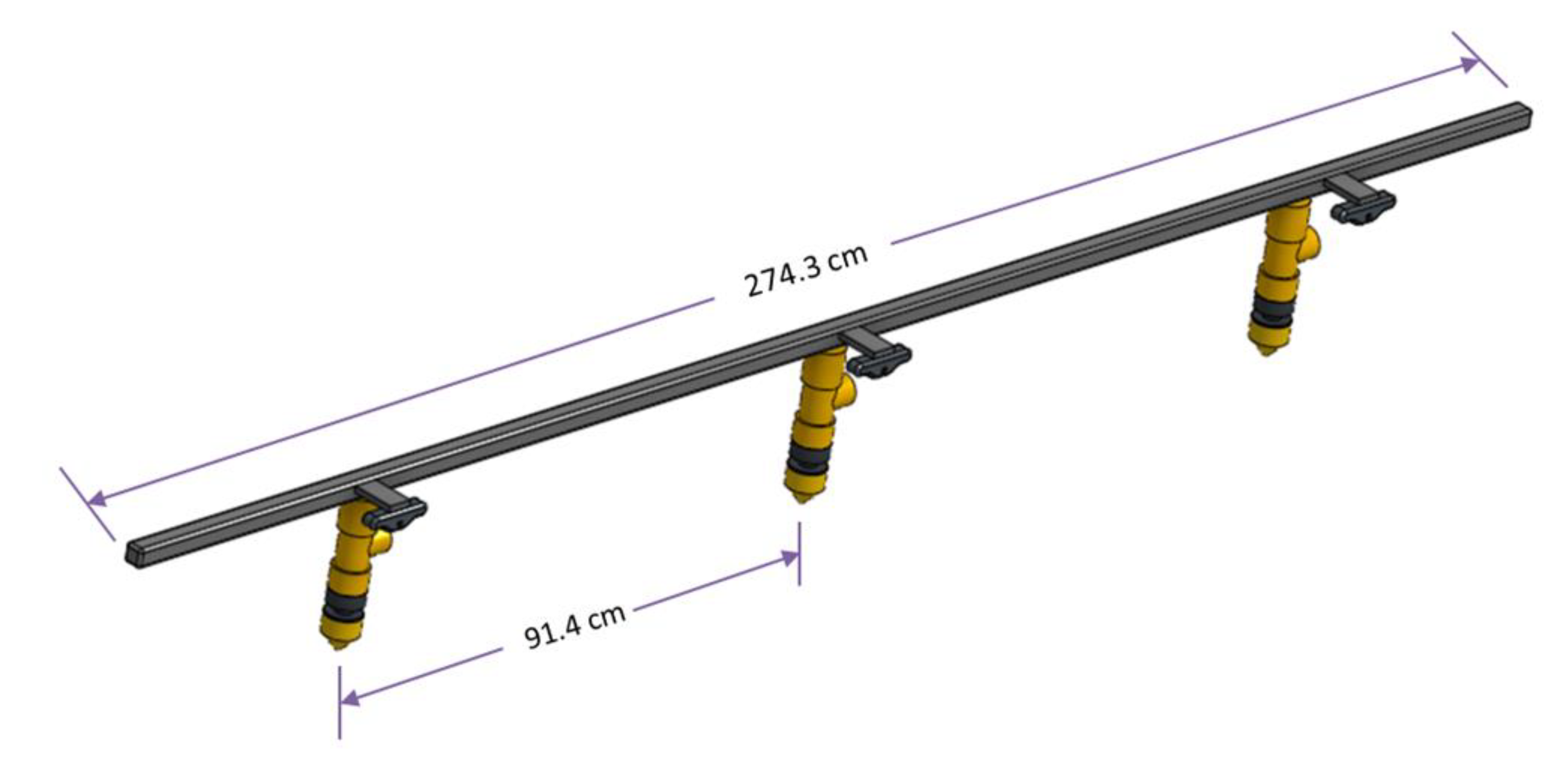
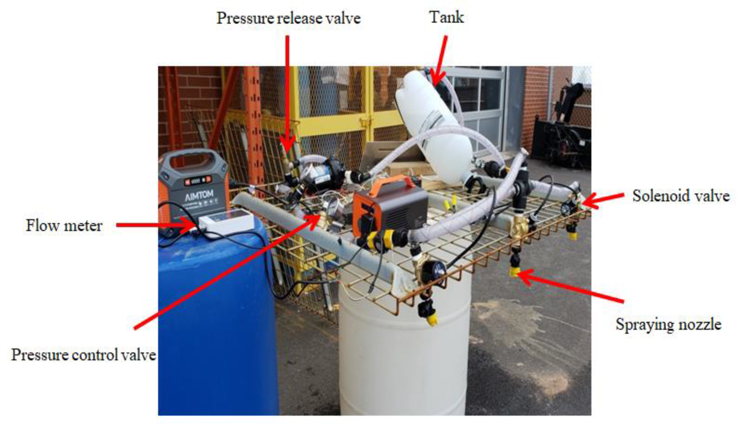
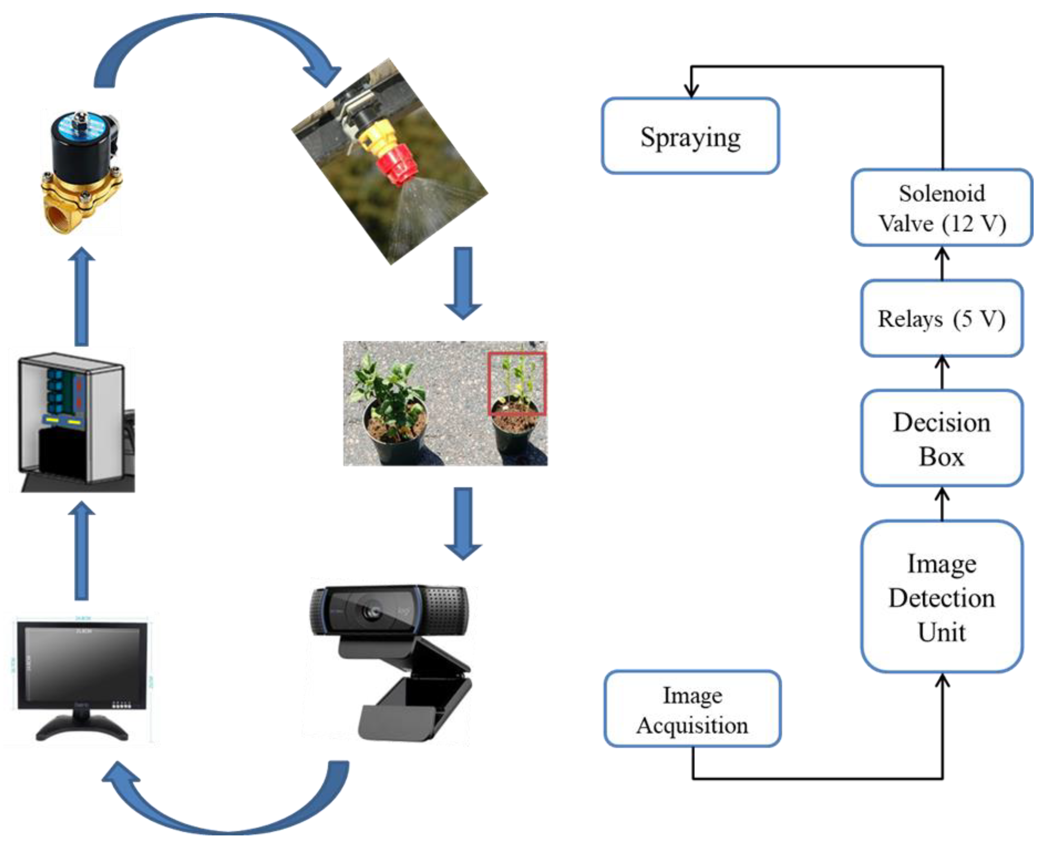
2.1. Hardware Development

A motorized farm buggy was developed in the Faculty of Sustainable Design Engineering Laboratory and equipped with SVRS accessories (Table 1). The buggy had 0.91 m of ground clearance (based on maximum potato plant height) with 0.30 m adjustability to accommodate variations of potato plant height at different growth stages. It was 0.89 m wide with tires spaced as per row spacing of potato crop. The length of the buggy was kept at 1.8 m to allow adequate space for an operator, engine, and necessary hardware. The buggy was equipped with the hardware listed in Table 1 and labeled in Figure 1.
A gasoline engine was used to power the SVRS. Power supply-1 was used to turn the electric solenoid valves on or off, and to charge the water flow meter. Power supply-2 was spared for the control unit and the computer screen. Power supply-3 was used for running the water pump. These power supplies were powered by rechargeable batteries of 110 V input voltage and 12, 5, and 110 V output voltages, respectively. Distance between the two adjacent spraying nozzles and two cameras was kept 0.91 m to cover one row of potato crop with one nozzle and camera (Figure 2). The total width of the sprayer boom was 2.74 m that allowed the mounting of three cameras and three nozzles.
A diaphragm pump with a maximum discharge flow of 15 lpm (liters per minute) and a maximum pressure of 414 kPa was used to supply the water for spraying nozzles. A pressure relief bypass valve was used to avoid backflow of water towards the supply tank and to maintain the flow toward nozzles in case of one or more nozzles closes when the sprayer does not detect any target. Three electric solenoid valves were used to actuate the nozzles following the signals sent by the control system. Three webcams were mounted at the heights and positions of spray nozzles to capture the images in real-time for further processing. Height from the ground level and distance between two adjacent cameras were adjusted to obtain the zero overlap between the views of cameras. Two emergency (on/off) switches, one for the sprayer engine and the second for the pump were installed on the front side of the sprayer. Relays, Arduino mega and ZOTAC Mini PC, were mounted in a control box. All the cameras were attached with a ZOTAC Mini PC by USB cables. An LCD panel was mounted at the right front side of the sprayer and attached to the ZOTAC Mini PC by HDMI cable (Figure 1).

2.2. Calibration of SVRS Components

A calibration bed was developed to calibrate components of the sprayer (Figure 3). Nozzles, flow meter and pressure control valves were calibrated using the calibration bed. A speedometer was calibrated after installing all the components on the buggy.

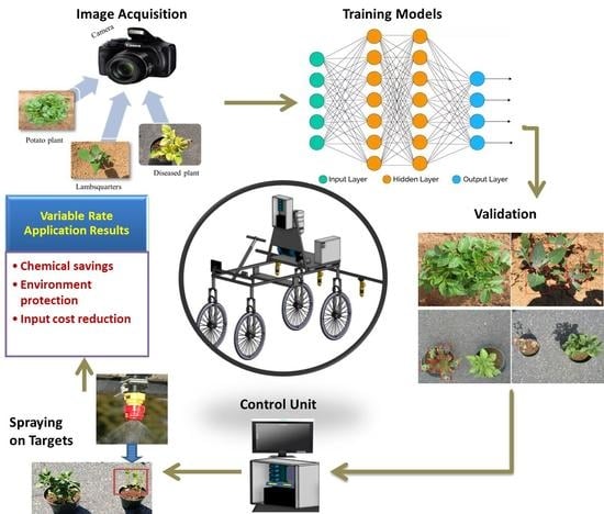
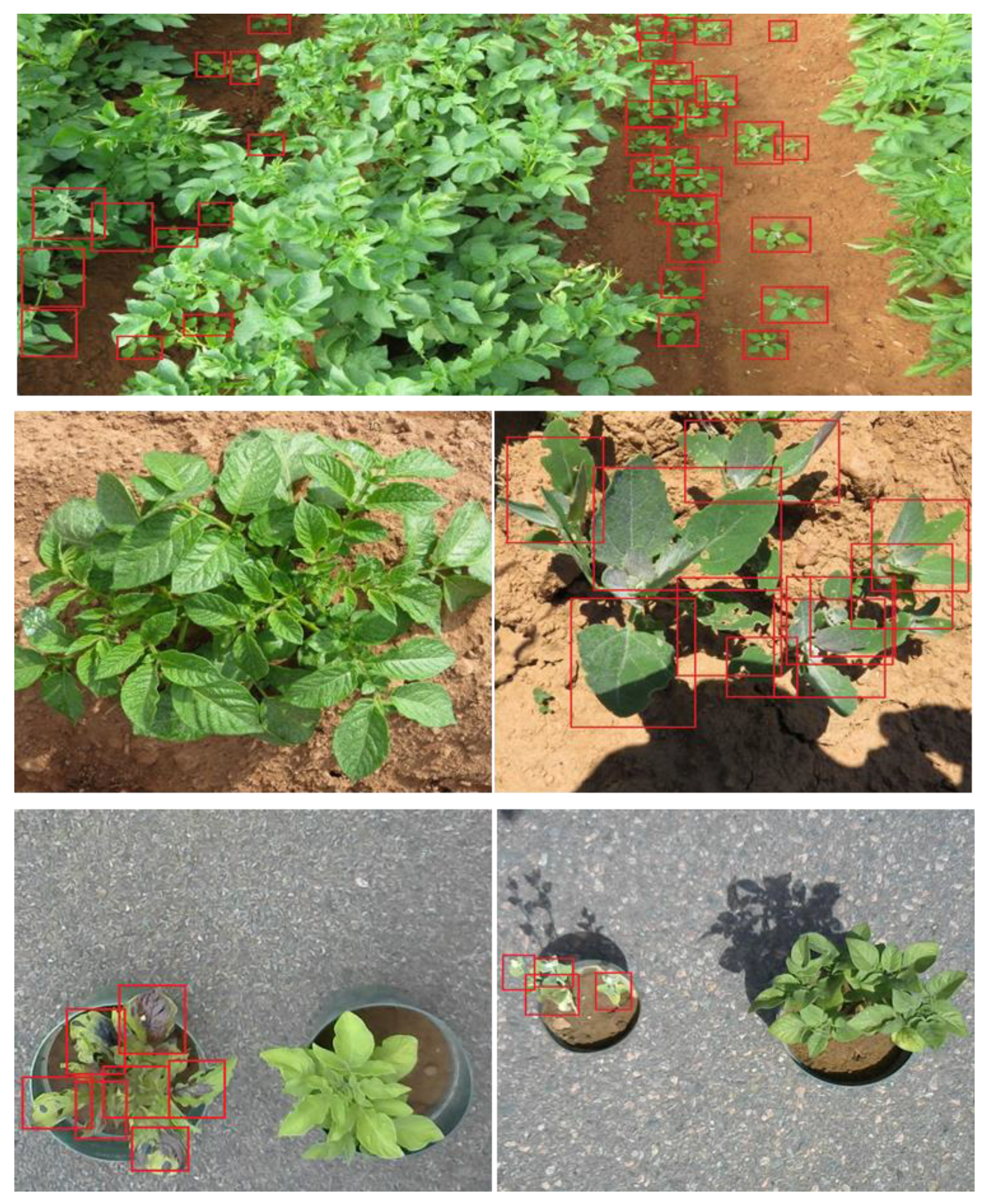
2.3. Image Acquisition

Two types of cameras (Canon PowerShot SX540 HS camera and Logitech C270 HD Webcam) were used to capture the images of lambsquarters (Chenopodium album) weed and potato (Solanum tuberosum L.) plants. The images were captured from three fields on Prince Edward Island at Winsloe North (46°21′24.47′′ N, 63°12′4.99′′ W), Agriculture and Agri-Food Canada, Harrington Research Station (46°20′59.2′′ N, 63°09′08.2′′ W), and 225 Highway (46°14′57.64′′ N, 63°11′46.46′′ W) and two fields in New Brunswick at Florenceville (46°19′5.38′′ N, 67°37′1.7′′ W), and Lavasque (47°6′5.53′′ N, 67°46′44.55′′ W). Ten thousand images of lambsquarters and the Russet Burbank variety of potato plants were taken from the potato fields.
Weather conditions of the three fields on Prince Edward Island were the same. The climate of Prince Edward Island is humid. Its winter season is long with a relatively shorter summer season. During the winter, the island receives storms and blizzards originating from the North Atlantic or the Gulf of Mexico. Springtime temperatures are cool, when the ice generally melts in late April. The summers are moderately warm as the daytime temperature occasionally reaches as high as 30 °C as the island receives the heaviest rainfall spells of the year during late autumn and during early winter.
Potato seeds were sown during late May and harvested during early October. Both fields were under conventional management practices and received traditionally recommended agronomic practices and amounts of agrochemicals for enhancing tuber yield, and for protecting the crop from weeds and diseases over the past decade. The cultivation in both the fields was rainfed and no supplemental irrigation was provided to the crop. Fertilization was the same in both fields as per local recommendations. The soils of the potato fields are sandy loams (Orthic Humo-Ferric Podzol) with large gravel and stones content, and with more than 2% of soil organic matter (SOM). The sandy soils have good drainage, aeration and thus can result in drought stress in the absence of supplemental irrigation. The weather, soil, growing season, and agronomic practices of New Brunswick fields were not different from the fields of Prince Edward Island.
About 200 plants of lambsquarters and 200 for potato plants of the same genotype as those of fields plants were planted in a 50:50 mix of Harrington (Prince Edward Island) field soil (Orthic Humo-Ferric Podzol; SOM 3%, and pH 6.6) and play sand. Soil and sand were heat-sterilized at 120 °C prior to use. Two sizes of pots were used to randomly grow lambsquarters weed and potato plants under general agronomic practices. The large pots had 16.5 cm upper diameter, 12.5 cm lower diameter, and 14 cm height. The small pots had a 12.8 cm upper diameter, 10.2 cm lower diameter, and 11.5 cm height. The pots were placed in the greenhouse of Agriculture and Agri-Food Canada.
Out of 400 plants of weed and potato, 310 plants were used for the model’s training purpose, and the remaining 90 plants (potato = 30, disease = 30, and weed = 30) were used for lab testing of SVRS. Two thousand images of weed and potato plants were captured using 310 plants grown in the greenhouse. All the images were taken at different growth stages of weed and potato plants to cover variations in the structure, color, and other physical features of lambsquarters and potato plants during their life cycle/growing season. The monthly temperature ranges for the growing season’s months; i.e., May, June, July, August, September, and October, were 5.00–18.0, 11.0–22.0, 15.0–24.0, 17.0–22.0, 9.00–22.0, and 4.00–16.0 °C, respectively. The first set of images were taken at the end of sprout development between days 7–29 after seedlings emergence (Growth Stage I). The second set of images was taken during the vegetative growth (Growth Stage II) on days 30–49 of the growing season. The third and fourth sets of images were taken during tuber initiation (Growth Stage III) and tuber bulking (Growth Stage IV) on days 50–70 and 70–125, respectively.
Altogether, 12,000 images were taken of potato plants and lambsquarters. Additionally, 12,000 more images of simulated diseased plants were captured. A dark brown color liquid was spread over the potato plants to mimic early blight disease symptoms due to the unavailability of diseased plants. Mixed images (images taken from different fields and from green house plants) were used for training of models on weeds and diseased mimicked plants. These images were taken at different times of the day, under varying light intensities (Table 2), at different heights from the ground level and from different angles to capture every possible setting for DL models.

2.4. Training of Models

All the images were resized to 1280 × 720 pixels, using Irfanview (Version 5.54) software, and labeled using Yolo Mark (https://github.com/AlexeyAB/Yolo_mark) tool. YOLO (you only look once) is a real-time object detection algorithm. It is a smart CNN that applies a single neural network to the full image, followed by dividing the image into regions to predict bounding boxes and probabilities for each region. These bounding boxes are weighted by the predicted probabilities. The advanced version of YOLO is YOLO (version 3), generally denoted as YOLOv3. The YOLOv3, which runs significantly faster than other detection methods with comparable performance. Tiny-YOLOv3 is a simplified model of YOLOv3, which reduces the depth of the convolutional layer. Its running speed has been greatly improved, although the detection accuracy has decreased, but to an acceptable limit.
The annotations saved by using Yolo Mark tool are in the format acceptable by YOLO (Figure 4). The ratio of training and testing validation images was 70:30 for both weed and simulated diseased image datasets. The images used for training were not used during testing. All the training experiments were performed using GPU (Nvidia GTX 1080 Ti) on Ubuntu 16.04. YOLO and tiny-YOLO algorithms developed by Redmon and Farhadi [32] were used to train the model using the Darknet framework. Tiny-YOLO is the simplified version of YOLO, which is faster but less accurate in comparison with YOLO [33]. The YOLO models were trained using a learning rate of 0.001, batch size of 32, image size of (416 × 416), the momentum of 0.95, weight decay of 0.0005, and iterations ranging from 6000 to 9000. Tiny-YOLOv3 and YOLOv3 were used to train the weed and simulated diseased plant detection datasets using the Darknet framework.

2.5. Evaluation Indicators

The parameters were used to evaluate the performance of neural networks [20] included precision, recall, F1Score, intersection over union (IOU), and mean average precision (mAP). Precision shows the effectiveness of neural networks in the identification of positive labels (the correct identification of targets). The best precision is considered at 1.0; whereas the poor precision is at 0.0. It was calculated as Precision = (TP/(TP + FP). Recall measures how the neural network identifies the targets. Its values reflect correctness of identification of weeds, simulated diseased, and healthy plants in this study. Its value varies from 0 to 1 and can be calculated as Recall = TP/(TP + FN). F1Score measures the harmonic mean of precision and recall, and gives the accuracy of detecting positive labels by neural network. The best F1Score is 1.0, the worst is 0. It can be calculated as F1Score = (2 × Precision × Recall)/(Precision + Recall). Intersection over Union measures the accuracy of detecting corresponding objects in a specific data set. Its value ranges from −1 to +1, and it can be calculated as IOU = TP/(FP + TP + FN). The mean average precision is the product of precision and recall of the detected bounding boxes. Its value varies from 0 to 100. The higher the number, the better it is. The mAP is measured by using the equation:
  mAP = k = 1 n P ( k ) Δ r ( k )
where P(k) is the precision at threshold k and Δr(k) is the change in recall.

2.6. Development of Models

The functions of SVRS were automated with a relay and microcontroller using a serial connection with python script. As per development, the trained models infer the results in the form of bounding boxes around the targets after image acquisition by cameras. Detected targets create the signal for the microcontroller, which activates the relays and solenoid valves. As the solenoid valve opens the spraying nozzle is actuated and the spraying liquid is applied to the target. The computational unit and the microcontroller unit communicate using a USB connection. An Arduino script (that controls the valves) has been developed to read the serial data coming from the computational unit containing the “target to be sprayed” (weed or disease-infected plant) position. For example, when the target is detected, the 5 V signal goes to the relay through Arduino and actuates the nozzle for opening the 12 V solenoid valve. Conversely, if no target is captured by the cameras, no signal is received by the control unit, and in this consequence, the solenoid valves and spraying nozzles remain off and spraying liquid goes back to the tank through a pressure release valve (Figure 5).

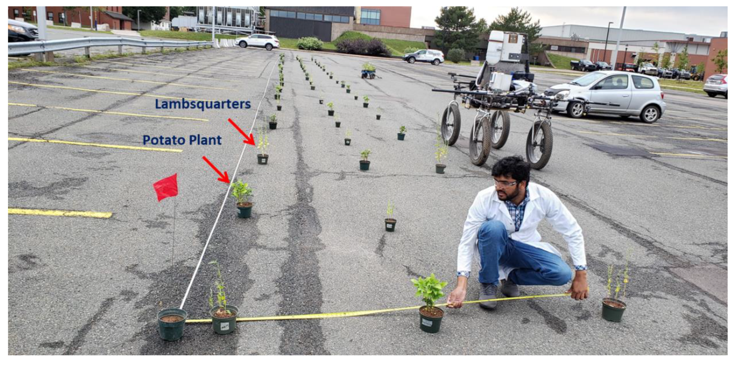
2.7. Design of the Laboratory Experiment

All the experiments were performed in the industrial parking lot of the Faculty of Sustainable Design Engineering of the University of Prince Edward Island, Canada. Lambsquarters and potato plants were grown in the greenhouse and brought to the lab to evaluate the performance of SVRS. Dark brown colors (multi-surface paint) were spread over the potato plants to mimic early blight disease symptoms. Plant pots were randomly arranged as three 60 m long and 2.74 m wide strips (Figure 6). Thirty targets (both weed and colored potato plants) and thirty non-targets (healthy potato plants) were randomly placed in the three rows. Laboratory testing was performed at different weather conditions using two spraying application techniques; i.e., VA and UA. Thus, for the weed detection experiment, the experiment design consisted of two treatments (VA and UA) and three levels of weather conditions (cloudy, partly cloudy, and sunny).
Rain-free days were chosen to test the SVRS for VA and UA performances. The values of temperature and light intensity recorded during the testing conditions of cloudy, partly cloudy, and sunny are given in Table 2. The same experimental design was revised for the simulated diseased plant detection experiments. The response variable evaluated in this study was the quantity of spraying liquid (liters) by VA and UA. Water was used as the spraying liquid during all trials to ensure the experimental approach to be environmentally friendly. All the experiments were conducted at 310 kPa pressure of spraying liquid. All the experiments were repeated six times with the ground speed of the sprayer’s buggy moving at 5 km h−1. The speed of the sprayer was constantly observed on the speedometer.

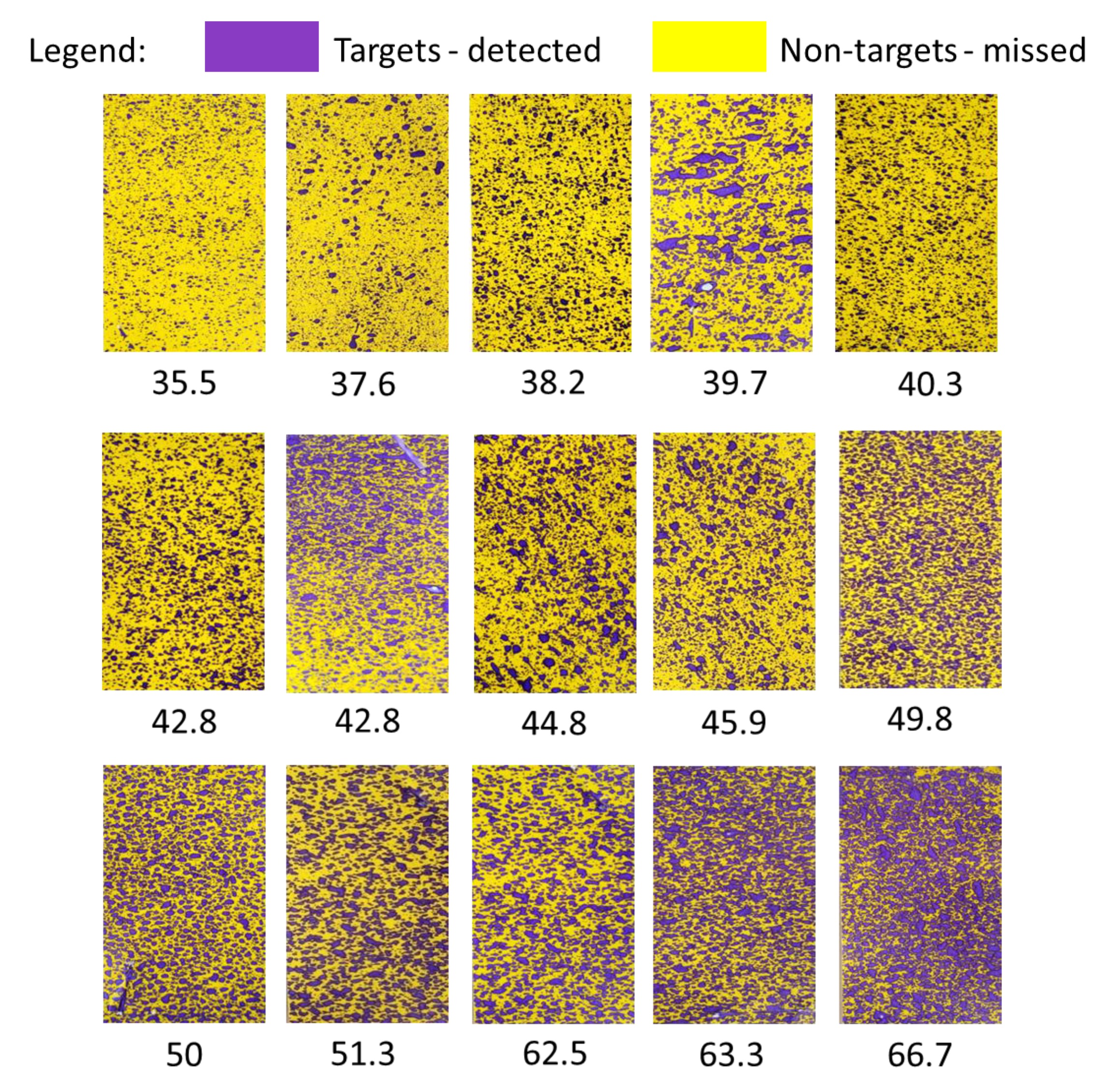
2.8. Measurement of Spraying Patterns and Percent Area Coverage

Water sensitive papers were stapled on the target and non-target plants to measure the spraying pattern and percent area coverage for SVRS during UA and VA of the spraying liquids. Custom software written in C++ language was used to process the water-sensitive papers. Images of the water-sensitive papers were used in bmp format to calculate the percent blue ratio by dividing number of blue pixels in the image by the number of total pixels in the image multiplied by 100. The percent blue ratio was used to represent the percentage area coverage of a chemical application technology.

2.9. Statistical Analysis

Both weed and disease infected plant detection experiments were designed under two-factor factorial arrangements for two treatments (UA and VA) and three levels of weather conditions (cloudy, partly cloudy, and sunny) with six replications using a 2 × 3 factorial design. The spraying techniques and weather conditions were the two independent variables with volume consumption of spraying liquid as a response variable (Table 2). Two-way (ANOVA) was run to examine the effects of treatments and weather conditions on the quantity of spraying liquid consumed. By using ANOVA, the differences in mean values were evaluated.
The group means were compared with the Fisher LSD comparisons test. Minitab 19 (Pennsylvania State University, State College, PA, USA: Minitab, Inc.) was used in the calculation of ANOVA and multiple means comparisons tests. The t-test was applied to analyze the water-sensitive paper results to observe the percent area coverage using VA and UA techniques. The same software was used to run the Student t-test for the water-sensitive papers. The Student t-test is widely used to compare the mean of two groups of samples (chemical volume consumption by VA and UA techniques in this case). Therefore, it was used to evaluate if the means of the two sets of data (VA and UA) were statistically significantly different from each other.
t = m 1 m 2 x 2 n 1 + x 2 n 2
where m1 and m2 are means of chemical volume consumption by VA and UA techniques, n1 and n2 represent size of VA and UA data, respectively. An estimator of the common variance of the two samples is represented by x2, which was calculated as:
x 2 = ( x m 1 ) 2 +   ( x m 2 ) 2 d f
where x is the individual observation. Once the t-test statistic value was determined, it was compared with values in t-test table, the critical value of the Student’s t distribution corresponding to the significance level alpha of the choice (i.e., 5%). The degrees of freedom (df) used in this test were calculated as:
d f = n 1 + n 2 2

3. Results

3.1. Training and Detection of Deep Learning Models

For both datasets (weed and simulated diseased potato plants) YOLOv3 performed comparatively better than tiny-YOLOv3 with respect to accuracy for both weed and simulated diseased plants datasets. Since the inference speed of tiny-YOLOv3 was considerably higher than the speed of YOLOv3, due to the high value of FPS, the tiny-YOLOv3 model was finalized to deploy in the SVRS. Redmon and Farhadi [32] also recommended the tiny-YOLOv3 for real-time performance over YOLOv3 due to inference speed. The mAP values were recorded as 78.2 and 93.2% for tiny-YOLOv3 and YOLOv3 models, respectively, for the weed dataset. Similarly, the mAP values were 76.4 and 91.4% for tiny-YOLOv3 and YOLOv3, respectively, for the simulated diseased plants dataset (Table 3). A similar trend was observed for other statistical significance indicators, i.e., precision, recall and F1Score values for simulated diseased plants dataset using these models (Table 3).

3.2. Pervormance Evaluation of SVRS

During the weed detection experiment, a significant difference (p < 0.05) in volume consumption of spraying liquid was recorded between VA and UA spraying techniques (Table 4). However, a non-significant difference (p > 0.05) in volume consumption of spraying liquid was observed under different weather conditions for the VA or UA spraying techniques. Similarly, there was a non-significant interaction (spraying application techniques × weather conditions) on volume consumption (p > 0.05), indicating all the interactions between spraying application techniques and weather conditions were statistically the same. By using the Fisher LSD comparison, it was found that the volume consumption for UA was significantly higher than the VA during the weed detection experiment. A similar trend was observed in simulated diseased plant detection experiments.
In the simulated diseased plant detection experiment, the percent savings of the applied liquids were 47.79, 48.67, and 48.48% for cloudy, partly cloudy, and sunny conditions, respectively. There was a non-significant difference (p > 0.05) in volume consumption of spraying liquid under different light conditions for both spraying techniques. During the weed detection experiment, relatively less percent saving of spraying liquid was recorded (Table 5).
A two-way ANOVA (Table 6) was run to examine the effects of treatments and weather conditions on volume consumption of spraying liquid. It was recorded that there was not a significant effect of volume consumption of spraying liquid under different weather conditions (cloudy, partly cloudy, and sunny) on spraying application techniques (p-value = 0.329).
The simple main effects analysis showed that there was a significant effect of spraying application techniques on volume consumption (p-value < 0.05) (Table 5). By using the Fisher LSD comparison, it suggested that the volume consumption for UA was significantly higher than the VA during the weed detection experiment. A similar trend was observed in simulated diseased plant detection experiments (Table 6). Statistical analysis showed that SVRS could significantly reduce the volume consumption of spraying liquid during weed and simulated diseased plant detection experiments.

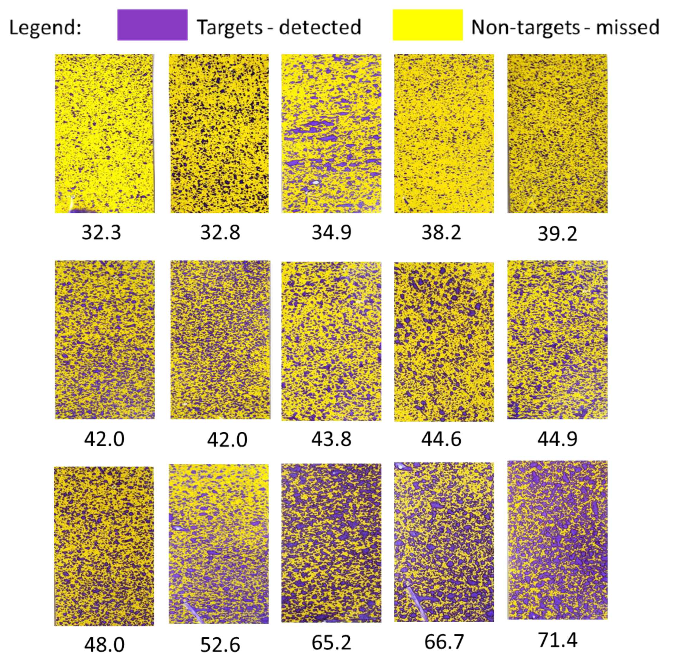
3.3. Spraying Patterns and Percent Area Coverage

Processing of the water-sensitive papers stapled with targets or non-targets reflected that the percent area coverage of the sprayed water-sensitive papers ranged from 32.3 to 71.4% and 35.5 to 66.7% for VA and UA techniques, respectively (Figure 7 and Figure 8, respectively). The percent area coverage of water-sensitive paper with the VA technique ranged from 0 to 2.89% in missing target areas.
By using a t-test, the probability value was calculated to be 0.83 for the weed detection experiment and 0.85 for the simulated diseased plant detection experiment during percent area coverage of UA and VA trials (Table 7). Similar results were reported by Esau et al. [6] for VR sprayers evaluated in wild blueberry fields. The p-value shows that there is a non-significant difference between VA and UA techniques with respect to spraying pattern and percent area coverage for targeted areas by using the SVRS, which means SVRS is applicable for the targeted application of spraying chemicals in the agricultural fields.

4. Discussion

The study results showed that the mAP value for the weed dataset was comparatively higher than for the simulated disease plants dataset. It means that it was easier to distinguish the weeds from potato plants as compared to simulated diseased plants from healthy potato plants. This may be because of the morphology of the plant leaves or because the disease was simulated and not real. Geometry and orientation of weed leaves are different from potato leaves, making their detection possible as compared to detection of disease symptoms on the same orientation of potato leaves. Partel et al. [27] also recorded precision = 71 and recall = 78 for weed detection using YOLOv3 models. Schumann et al. [34] found and reported similar results for the YOLOv3-spp network, which performed best with 91% recall, and 28.3 milliseconds inference time and could successfully identify the maturity stages of blueberries in the field.
The weather condition, especially those affecting light, affected the performance of the SVRS. For example, under cloudy conditions, the amount of volume consumption was relatively high during both weed and simulated diseased plant detection experiments, which might be due to some missing of targets (3–5%) during low-intensity light conditions. The possible reason for this may be a decrease in the quality of images under low light conditions, as also reported by Dobashi et al. [35].
Higher non-target detections (0–6.7%) were recorded in diseased plant detection experiments. It was probably due to similarity in shape of the targets and non-targets for weed and simulated diseased plant experiments. The reason for variation in percent area coverage might also be due to spray drift caused by high winds experienced during the performance evaluation tests. Very small percent area coverage could have resulted from spray drifting from adjacent nozzles or from the spray drifting from the front or back edge of the missing targets.
During the reported experiments, the product spraying flow/pressure was set as a standard pressure. The saving of chemicals may change if the product is sprayed on other pressures, but it has not been tested and confirmed in these experiments. In addition to the varying pressure and the light intensity, the results may vary with the prevailing temperature, the ground speed of the sprayer, and the type of weeds and diseased plant. Therefore, under the tested experimental conditions, the SVRS could be viable for site-specific applications of herbicides and fungicides in potato crops.

5. Conclusions

A variable-rate smart sprayer was designed, developed, and evaluated at a laboratory scale for site-specific application of spraying liquids. Nozzles, valves, and a speedometer were calibrated for better performance of the sprayer. Both DCNN models tiny-YOLOv3 and YOLOv3 performed adequately with respect to the accuracy, but the inference speed of tiny-YOLOv3 was considerably higher than the YOLOv3 model. It suggested deploying the tiny-YOLOv3 in SVRS. The SVRS successfully detected the weeds, simulated diseased plants, and green potato plants using tiny-YOLOv3 with Darknet framework. The VA technique of spraying liquid was significantly better than the UA. The SVRS was able to save 42 and 43% spraying liquids for weed and simulated diseased detection experiments, respectively. With the developed SVRS, the farmers would be applying the agrochemical using DL based sprayers under every weather condition. Water sensitive paper analysis showed that SVRS could be used to get good percent area coverage as in UA. More than 40% savings of spraying liquid showed that the SVRS has the potential to save input costs of spraying chemicals while helping to protect the environment. The work is in progress for some potential advances regarding field evaluation of the developed SVRS for spot-application of agrochemicals on weeds and diseased potato plants.

Author Contributions

Conceptualization: A.A.F., methodology: A.A.F., N.H., A.W.S., and Q.Z., software: A.A.F., N.H., A.W.S., and F.A., validation: A.W.S., A.M.-G., B.A. and Q.Z., formal analysis: T.E. and F.A., investigation: A.A.F., N.H., and F.A., resources: A.A.F. data curation: N.H., writing—original draft preparation: A.A.F., N.H., T.E., F.A., B.A., and Q.Z., writing—review and editing: A.A.F., N.H., A.W.S., A.M.-G., T.E., F.A., B.A., and Q.Z., supervision: A.A.F., A.W.S., A.M.-G., T.E., B.A., and Q.Z., project administration: A.A.F., funding acquisition: A.A.F. All authors have read and agreed to the published version of the manuscript.

Funding

This research was funded by the Natural Science and Engineering Research Council of Canada.

Acknowledgments

The authors are thankful to Ryan Barret (Research Coordinator; Prince Edward Island Potato Board), Joe Brennan and Khalil Al-Mughrabi (New Brunswick Potato Transformation Initiative), and the Precision Agriculture Team at the University of Prince Edward Island for their cooperation and assistance during the experiment.

Conflicts of Interest

The Authors declare no conflict of interest.

References

  1. Swanson, N.L.; Leu, A.; Abrahamson, J.; Wallet, B. Genetically engineered crops, glyphosate and the deterioration of health in the United States of America. J. Org. Syst. 2014, 9, 6–37. [Google Scholar]
  2. López-Granados, F.; Torres-Sánchez, J.; Serrano-Pérez, A.; de Castro, A.; Mesas-Carrascosa, F.; Peña, J.M. Early season weed mapping in sunflower using UAV technology: Variability of herbicide treatment maps against weed thresholds. Precis. Agric. 2016, 17, 183–199. [Google Scholar] [CrossRef]
  3. Jurado-Expósito, M.; López-Granados, F.; Gonzalez-Andujar, J.L.; Torres, L.G. Characterizing Population Growth Rate of in Wheat-Sunflower No-Tillage Systems Modelling the effects of climate change on weed population dynamics View project. Crop Sci. 2005, 45, 2106–2112. [Google Scholar] [CrossRef] [Green Version]
  4. Lamichhane, J.R.; Dachbrodt-Saaydeh, S.; Kudsk, P.; Messéan, A. Toward a reduced reliance on conventional pesticides in European agriculture. Plant Dis. 2016, 100, 10–24. [Google Scholar] [CrossRef] [PubMed] [Green Version]
  5. Creech, C.F.; Henry, R.S.; Werle, R.; Sandell, L.D.; Hewitt, A.J.; Kruger, G.R. Performance of Postemergence Herbicides Applied at Different Carrier Volume Rates. Weed Technol. 2015, 29, 611–624. [Google Scholar] [CrossRef]
  6. Esau, T.J.; Zaman, Q.U.; Chang, Y.K.; Schumann, A.W.; Percival, D.C.; Farooque, A.A. Spot-application of fungicide for wild blueberry using an automated prototype variable rate sprayer. Precis. Agric. 2014, 15, 147–161. [Google Scholar] [CrossRef]
  7. Dammer, K.H.; Wollny, J.; Giebel, A. Estimation of the Leaf Area Index in cereal crops for variable rate fungicide spraying. Eur. J. Agron. 2008, 28, 351–360. [Google Scholar] [CrossRef]
  8. Netland, J.; Balvoll, G.; Holmøy, R. Band spraying, selective flame weeding and hoeing in late white cabbage part II. Acta Hortic. 1994, 235–244. [Google Scholar] [CrossRef]
  9. Miller, P.C.H. Patch spraying: Future role of electronics in limiting pesticide use. Pest Manag. Sci. 2003, 59, 566–574. [Google Scholar] [CrossRef]
  10. Abdulridha, J.; Ehsani, R.; Abd-Elrahman, A.; Ampatzidis, Y. A remote sensing technique for detecting laurel wilt disease in avocado in presence of other biotic and abiotic stresses. Comput. Electron. Agric. 2019, 156, 549–557. [Google Scholar] [CrossRef]
  11. Zaman, Q.U.; Esau, T.J.; Schumann, A.W.; Percival, D.C.; Chang, Y.K.; Read, S.M.; Farooque, A.A. Development of prototype automated variable rate sprayer for real-time spot-application of agrochemicals in wild blueberry fields. Comput. Electron. Agric. 2011, 76, 175–182. [Google Scholar] [CrossRef]
  12. Qiongyan, L.; Cai, J.; Berger, B.; Okamoto, M.; Miklavcic, S.J. Detecting spikes of wheat plants using neural networks with Laws texture energy. Plant Methods 2017, 13, 83. [Google Scholar] [CrossRef] [PubMed] [Green Version]
  13. Pound, M.P.; Atkinson, J.A.; Wells, D.M.; Pridmore, T.P.; French, A.P. Deep Learning for Multi-Task Plant Phenotyping Figure 1: A Selection of Results from Our Deep Network Locating Spikes (Middle) and Spikelets (Bottom) on the ACID Dataset. 2017. Available online: http://plantimages.nottingham.ac.uk/ (accessed on 1 February 2020).
  14. Yang, X.; Sun, M. A Survey on Deep Learning in Crop Planting. IOP Conf. Ser. Mater. Sci. Eng. Inst. Phys. Publ. 2019, 490, 062053. [Google Scholar] [CrossRef]
  15. Milioto, A.; Lottes, P.; Stachniss, C. Real-time blob-wise sugar beets vs weeds classification for monitoring fields using convolutional neural networks. ISPRS Ann. Photogramm. Remote Sens. Spat. Inf. Sci. 2017, 4, 41–48. [Google Scholar] [CrossRef] [Green Version]
  16. Lu, J.; Hu, J.; Zhao, G.; Mei, F.; Zhang, C. An in-field automatic wheat disease diagnosis system. Comput. Electron. Agric. 2017, 142, 369–379. [Google Scholar] [CrossRef] [Green Version]
  17. Liakos, K.G.; Busato, P.; Moshou, D.; Pearson, S.; Bochtis, D. Machine learning in agriculture: A review. Sensors 2018, 18, 2674. [Google Scholar] [CrossRef] [PubMed] [Green Version]
  18. Hirz, M.; Walzel, B. Sensor and object recognition technologies for self-driving cars. Comput. Aided. Des. Appl. 2018, 15, 501–508. [Google Scholar] [CrossRef] [Green Version]
  19. Ren, S.; He, K.; Girshick, R.; Sun, J. Faster R-CNN: Towards Real-Time Object Detection with Region Proposal Networks. IEEE Trans. Pattern Anal. Mach. Intell. 2017, 39, 1137–1149. [Google Scholar] [CrossRef] [Green Version]
  20. Zhao, K.; Ren, X. Small Aircraft Detection in Remote Sensing Images Based on YOLOv3. IOP Conf. Ser. Mater. Sci. Eng. Inst. Phys. Publ. 2019, 533, 012056. [Google Scholar] [CrossRef]
  21. Shahud, M.; Bajracharya, J.; Praneetpolgrang, P.; Petcharee, S. Thai traffic sign detection and recognition using convolutional neural networks. In Proceedings of the 2018 22nd International Computer Science and Engineering Conference (ICSEC), Chiang Mai, Thailand, 21–24 November 2018. [Google Scholar] [CrossRef]
  22. Xiao, D.; Shan, F.; Li, Z.; Le, B.T.; Liu, X.; Li, X. A Target Detection Model Based on Improved Tiny-Yolov3 under the Environment of Mining Truck. IEEE Access. 2019, 7, 123757–123764. [Google Scholar] [CrossRef]
  23. Tian, L. Development of a sensor-based precision herbicide application system. Comput. Electron. Agric. 2002, 36, 133–149. [Google Scholar] [CrossRef]
  24. Pathak, A.R.; Pandey, M.; Rautaray, S. Application of Deep Learning for Object Detection. Procedia Comput. Sci. 2018, 132, 1706–1717. [Google Scholar] [CrossRef]
  25. Han, S.; Shen, W.; Liu, Z. Deep Drone: Object Detection and Tracking for Smart Drones on Embedded System; Stanford University: Stanford, CA, USA, 2016; pp. 1–8. [Google Scholar]
  26. Tijtgat, N.; Van Ranst, W.; Volckaert, B.; Goedemé, T.; De Turck, F. Embedded real-time object detection for a UAV warning system. In Proceedings of the 2017 IEEE International Conference on Computer Vision Workshops (ICCV), Venice, Italy, 22–29 October 2017; pp. 2110–2118. [Google Scholar]
  27. Partel, V.; Charan Kakarla, S.; Ampatzidis, Y. Development and evaluation of a low-cost and smart technology for precision weed management utilizing artificial intelligence. Comput. Electron. Agric. 2019, 157, 339–350. [Google Scholar] [CrossRef]
  28. Ampatzidis, Y.; De Bellis, L.; Luvisi, A. iPathology: Robotic applications and management of plants and plant diseases. Sustainability 2017, 9, 1010. [Google Scholar] [CrossRef] [Green Version]
  29. Samseemoung, G.; Soni, P.; Suwan, P. Development of a variable rate chemical sprayer for monitoring diseases and pests infestation in coconut plantations. Agriculture 2017, 7, 89. [Google Scholar] [CrossRef] [Green Version]
  30. Fernández-Quintanilla, C.; Peña, J.M.; Andújar, D.; Dorado, J.; Ribeiro, A.; López-Granados, F. Is the current state of the art of weed monitoring suitable for site-specific weed management in arable crops? Weed Res. 2018, 58, 259–272. [Google Scholar] [CrossRef]
  31. Möller, J. Computer Vision—A Versatile Technology in Automation of Agriculture Machinery. J. Agric. Eng. 2010, 47, 28–36. [Google Scholar]
  32. Redmon, J.; Farhadi, A. YOLOv3: An Incremental Improvement. 2018. Available online: http://arxiv.org/abs/1804.02767 (accessed on 20 January 2020).
  33. Zhang, P.; Zhong, Y.; Li, X. SlimYOLOv3: Narrower, faster and better for real-time UAV applications. In Proceedings of the 2019 IEEE International Conference on Computer Vision Workshops (ICCV), Seoul, Korea, 27 October–2 November 2019; pp. 37–45. [Google Scholar]
  34. Schumann, A.W.; Mood, N.S.; Mungofa, P.D.; MacEachern, C.; Zaman, Q.U.; Esau, T. Detection of three fruit maturity stages in wild blueberry fields using deep learning artificial neural networks. In Proceedings of the 2019 ASABE Annual International Meeting. American Society of Agricultural and Biological Engineers, Boston, MA, USA, 7–10 July 2019; p. 1. [Google Scholar] [CrossRef]
  35. Dobashi, Y.; Yamamoto, T.; Nishita, T. Efficient rendering of lightning taking into account scattering effects due to clouds and atmospheric particles. In Proceedings of the Ninth Pacific Conference on Computer Graphics and Applications Pacific Graphics, Tokyo, Japan, 16–18 October 2001; pp. 390–399. [Google Scholar]
Figure 1. A model for a smart variable rate sprayer labeled for its equipment and accessories.
Remotesensing 12 04091 g001
Figure 2. Spraying boom with nozzles and cameras to account for the distance between the two rows of potato plants cultivated in furrows.
Remotesensing 12 04091 g002
Figure 3. Calibration bed to calibrate the nozzles and different valves of a smart variable rate sprayer.
Remotesensing 12 04091 g003
Figure 4. Processed images of lambsquarters, simulated diseased, and healthy potato plants.
Remotesensing 12 04091 g004
Figure 5. Flow chart of a smart variable rate sprayer for real-time detection of required weed or simulated diseased plants and targeted application of agrochemicals.
Remotesensing 12 04091 g005
Figure 6. Design of the laboratory experiment for testing of smart variable rate sprayer. The experimental setup consisted of 60 m long and 2.74 m wide strips of randomly arranged healthy, simulated diseased, and weed plants.
Remotesensing 12 04091 g006
Figure 7. Processed images of water-sensitive papers for variable rate application treatment showing the percent areas coverage of targets (purple) and non-target (yellow) missed during variable rate application of the spraying liquid. The numbers below each image of the water-sensitive paper represent blue ratio; i.e., ratio (to be considered as percent area coverage of variable rate application treatment) of image pixels turned into blue after receiving the spraying liquid (target detected) to the total image pixels.
Remotesensing 12 04091 g007
Figure 8. Processed images of water-sensitive papers for uniform application treatment showing the percent areas coverage of targets (purple) and non-target (yellow) missed during uniform application of the spraying liquid. The numbers below each image of the water-sensitive paper represent blue ratio; i.e., ratio (to be considered as percent area coverage of uniform application treatment) of image pixels turned into blue after receiving the spraying liquid (target detected) to the total image pixels.
Remotesensing 12 04091 g008
Table 1. The types of equipment used in a smart variable rate sprayer with their specifications.
NoEquipmentSpecificationNoEquipmentSpecification
1ZOTAC Mini PCGeForce GTX 105011Bypass valve12.7 mm Bypass Relief Valve; 0–1724 kPa
2Relay module8 channels12Pressure gauge Liquid Filled Pressure Gauge 1103 kPa
3Arduino megaElegoo MEGA 2560 R313Pressure control valveWater Pressure Regulator Valve
4LCD screen10 Inch IPS LCD14Three nozzlesTeeJet XR Extended Range Spray Nozzle
5SpeedometerAnalog15FilterHypro 3350–0079 Nylon Line Strainer
6Three solenoid valvesBrass Solenoid Valve DC 12 V16Pump12 V Diaphragm Pump – 15 lpm
7Three camerasLogitech C920 Webcam HD Pro17Shut off valveOn/Off
8Power supply-142,000 mAh 155 Wh Power Station18Flow meterWater Flow Control Meter LCD Display Controller
9Power supply-2230 Wh 62,400 mAh Power Station19Supply tank15 l
10Power supply-312 V 18 Ah SLA Battery20Gasoline engine7.5 l
Table 2. Light intensity values at different weather conditions under which the sprayer was tested.
ExperimentTestReplicationTargetWeather ConditionTemperature
Range
°C
Light Intensity
(Lux) × 100
Weed
Detection
16Weed plantCloudy9.50–13.0100–360
26Partly cloudy13.5–19.0400–545
36Sunny16.8–25.0550–1000
Simulated
Diseased Plant
Detection
46Simulated
diseased
plant
Cloudy10.0–12.5100–350
56Partly cloudy14.0–17.5430–468
66Sunny16.0–24.5500–1000
Table 3. Results of tiny-YOLOv3 and YOLOv3 models for both weed and simulated diseased plants datasets.
DatasetsModelPrecisionRecallF1ScoremAP%FPS
Weed plantsTiny-YOLOv30.860.790.7878.230.0
Simulated diseased plantsTiny-YOLOv30.780.80.7576.430.5
Weed plantsYOLOv30.920.870.8593.214.6
Simulated diseased plantsYOLOv30.840.820.8391.415.6
mAP = mean average precision and FPS = frames per second.
Table 4. The two-way ANOVA results showing the effects of spraying techniques (the treatments) and weather conditions (cloudy, partly cloudy, and sunny) and their interaction (treatment × condition) on volume consumptions for spraying during weed and simulated disease experiments.
ExperimentResponse VariableSourceDFMean SquareF-Valuep-Value
Weed detectionVolume consumption (l)Treatment17.58262108.4<0.05
Condition20.00411.150.329
Treatment × condition20.00090.260.773
Error300.0036
Total35
Simulated diseased plant detectionVolume consumption (l)Treatment19.79062517.4<0.05
Condition20.00761.970.156
Treatment × condition20.002220.570.571
Error300.0038
Total35
DF = degree of freedom.
Table 5. Descriptive statistics for volume consumption of spraying liquid using two spraying techniques (treatment VA and UA) under three weather conditions (cloudy, partly cloudy, and sunny) for weed and simulated diseased plant detection experiments.
Weed Detection Experiment
Response VariableTreatmentConditionNMeanSDMinimumMaximum% Saving
Volume consumption (l)VACloudy61.21800.081.0851.32441.76
Partly Cloudy61.21120.061.111.32442.71
Sunny61.18870.031.1221.243.29
UACloudy62.09170.012.0762.108NA
Partly Cloudy62.11450.0722.2
Sunny62.09620.062.0042.17
Simulated Diseased Plant Detection Experiment
Volume consumption (l)VACloudy61.11180.071.0071.247.79
Partly Cloudy61.13030.051.061.2148.67
Sunny61.10470.051.0261.1848.47
UACloudy62.12970.022.12.153NA
Partly Cloudy62.20220.102.072.32
Sunny62.1440.032.12.19
VA = variable rate application; UA = uniform application; N = number of replications; SD = standard deviation.
Table 6. Two-way ANOVA comparison to observe the effect of different weather conditions (cloudy, partly cloudy and sunny) on spraying application techniques and their interactions for weed and simulated disease experiments using a smart variable rate sprayer at lab scale.
ExperimentResponse VariableSourceDFMean SquareF-Valuep-Value
Weed detectionVolume Consumption (l)Treatment17.58262108.4<0.05
Condition20.00411.150.329
Condition*Treatment20.00090.260.773
Error300.0036
Total35
Simulated diseased plant detectionVolume Consumption (l)Treatment19.79062517.4<0.05
Condition20.00761.970.156
Condition*Treatment20.002220.570.571
Error300.0038
Total35
DF = degree of freedom.
Table 7. Results of the t-test to compare the performance of the newly developed smart variable rate sprayer in comparison to uniform application.
ExperimentTreatmentNMeanSDSE Meanp-Value
Weed plants detectionUA1546.612.33.20.83
VA1547.429.872.5
Simulated diseased plants detectionUA1545.9810.912.70.85
VA1548.6210.012.2
UA = uniform application; N = number of observations; VA = variable rate application; SD = standard deviation; and SE = standard error.
Publisher’s Note: MDPI stays neutral with regard to jurisdictional claims in published maps and institutional affiliations.

