A Co-Operative Autonomous Offshore System for Target Detection Using Multi-Sensor Technology

Abstract

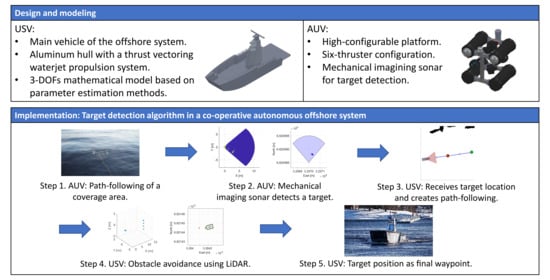
This article studies the design, modeling, and implementation challenges for a target detection algorithm using multi-sensor technology of a co-operative autonomous offshore system, formed by an unmanned surface vehicle (USV) and an autonomous underwater vehicle (AUV). First, the study develops an accurate mathematical model of the USV to be included as a simulation environment for testing the guidance, navigation, and control (GNC) algorithm. Then, a guidance system is addressed based on an underwater coverage path for the AUV, which uses a mechanical imaging sonar as the primary AUV perception sensor and ultra-short baseline (USBL) as a positioning system. Once the target is detected, the AUV sends its location to the USV, which creates a straight-line for path following with obstacle avoidance capabilities, using a LiDAR as the main USV perception sensor. This communication in the co-operative autonomous offshore system includes a decentralized Robot Operating System (ROS) framework with a master node at each vehicle. Additionally, each vehicle uses a modular approach for the GNC architecture, including target detection, path-following, and guidance control modules. Finally, implementation challenges in a field test scenario involving both AUV and USV are addressed to validate the target detection algorithm.

1. Introduction

In recent years, the use of autonomous offshore vehicles, which includes autonomous underwater vehicles (AUVs) and unmanned surface vehicles (USVs), for marine interventions has attracted increasing interest from research scientists, maritime industries, and the military. These interventions include several activities such as offshore surveillance, offshore target detection, seabed explorations, or search and rescue (SAR) missions. Additionally, the use of multi-robot platforms can improve the performance in these activities, as they can include above and below-water characterization. Regarding a multi-robot platform, Vasilijević et al. [1] presented the co-operative robotic system consisting of an AUV and a USV for ocean sampling and environmental monitoring. In [2], the study used a heterogeneous collaborative system of above, surface, and underwater robots to obtain a multi-domain awareness on a floating target. The heterogeneous system consists of a USV, an AUV, and an unmanned aerial vehicle (UAV). Additionally, Gu et al. [3] presented a homogeneous study, where a guidance and control law design method for coordinated path following of networked under-actuated robotic USVs under directed communication links. In [4], the control scenario simulated a homogeneous AUV fleet to study formation tracking control and collision-obstacle avoidance.

To accomplish the target detection in the offshore environment, the availability of accurate USV and AUV mathematical models is crucial for simulation study purposes, controller design, and development. The theoretical six-degrees-of-freedom (DOFs) dynamic model [5], based on nonlinear equations of motion, can be used for the design and modeling of the AUV. Equally, the USV can use the same dynamic model of the AUV but with reduced order for the three DOFs horizontal plane control (surge, sway, and yaw motions). Several tools can help to obtain the coefficients of the dynamic model equations and the necessary transfer functions of each vehicle. These tools can include the parameter estimation from MATLAB-Simulink [6], and the system identification (SI) [7,8], introduced to develop the mathematical model using field test data. In [9], SI of the maneuvering data determined the hydrodynamic coefficients of a USV. Also, the mathematical model of the USV includes the propulsion and power system. Commonly, the rudder and propeller, or waterjet propulsion systems provide the heading and the speed control of most existing USVs. In [10], a twin waterjet propelled USV was modeled based on SI, but it neglects the calculation for the dynamics of the propulsion system.

Target detection in offshore environments is a fundamental activity that combines different perception sensors. Numerous studies use passive (stereo cameras) or active (LiDAR or radar) perception methods to obtain situational awareness of a USV. Nonetheless, most of the obstacle detection methods rely on depth measurements, in which LiDAR sensors are the most reliable method of obtaining depth data. Correspondingly, sonar devices are still the most convenient option for collecting data on underwater environments. Mechanical imaging sonar, multibeam, profiler, or sidescan are some of the main sonar imaging and ranging devices. For the target detection with sonar devices, how detectable is a target is mainly dependent on the physical characteristics of the target and acoustic signal. Some studies use sonar devices for target detection capabilities, as in [11], where a profiler sonar was adopted for obstacle detection. According to [12], a method for underwater obstacle detection (standard buoy) was developed using forward-looking sonar and a probabilistic local occupancy grid.

Correct localization and navigation are crucial to ensure the accuracy of the gathered data for all these applications. Above the water surface, most of the autonomous systems rely on radio or global positioning and spread-spectrum communications, as a GPS-compass installed in the USV platform. However, those signals propagate only in short distances in an underwater scenario, where acoustic-based systems perform better. Regarding underwater navigation, the three fundamental methods are dead-reckoning (DR) and inertial navigation systems (INS), acoustic navigation, and geophysical navigation techniques [13]. These navigation methods require specific survey and navigation sensors installed in the AUV. The Girona 500 [14] is an example of AUV that performs the traditional dead-reckoning navigation utilizing a doppler velocity log (DVL) and a solid-state attitude and heading reference system (AHRS). Also, the absolute position can be obtained through a GPS when the vehicle is on the surface and using an ultra-short baseline (USBL) while underwater. The high-accuracy USBL system allows the localization of the AUV and the communication between the vehicle and the surface unit. In [15], the study provided a navigation algorithm for an underwater vehicle with a Kalman filter to estimate the error state via measurement residuals from aiding sensors. These aiding sensors incorporate an attitude sensor, a DVL, a long-baseline (LBL) system, and a pressure sensor. In acoustic navigation techniques, acoustic transponders and modems perform localization by measuring the time-of-flight of signals from acoustic beacons or modems. USBL navigation allows an AUV to localize itself relative to a USV, and it provides an efficient and reliable acoustic communication network [16]. In [17], the study presented the design and implementation of an USBL-aided navigation approach for an AUV in a two-parallel extended Kalman filter (EKF). It also includes the measurements provided by a DVL, a Visual Odometer, an inertial measurement unit (IMU), a pressure sensor, and a GPS.

Safe and adequate control of the offshore vehicles depends notably on proper guidance, navigation, and control (GNC) systems. This study adopts a path-following as the guidance system for both offshore platforms. The path-following approach is closer to practical engineering, and it is easier to implement than trajectory tracking. A generally used method for path-following in autonomous vehicles is the named line-of-sight (LOS) guidance. LOS guidance is classified as a three-point guidance scheme, involving a commonly stationary reference point along with the interceptor and the target [5]. In [18], the study developed a guidance-based algorithm for path-following using the LOS algorithm in offshore operations. Additionally, in [10], a path-following with obstacle avoidance based on the safety boundary box approach was implemented in a USV with a LOS-based guidance system.

Due to the co-operative offshore system in this study, it becomes necessary to fuse information obtained from the individual vehicles. Robot Operating System (ROS) has been an effective tool when working with multi-robot systems. This tool is a flexible framework for writing robot software and provides the tools to acquire sensors’ data, process it, and generate the necessary response for the vehicle actuators [19]. Multi-robot systems can either be centralized with a ROS master node at the ground control station (GCS) or decentralized with each autonomous vehicle (AV) running an independent ROS master. In the case of the decentralized control techniques, they are more flexible, profitable, and generally reduce the communication network requirements compared with centralized control [20]. However, they are also more challenging due to obstacles, uncertainties, and communication constraints, such as noises, delays, dropouts, or failures. In this case, the multi-master approach provides a solution where each vehicle keeps its own ROS master and also exchange the necessary information with other components of the multi-robot system. In [21], they proposed a package that efficiently developed multi-master architectures.

In the presented manuscript, the mathematical model of the USV consists of the simplified three DOFs dynamic model [5], where their parameters are obtained from field test data using the parameter estimation tool. Additionally, the waterjet model has been included in the mathematical model of the USV using data from the manufacturer and transfer functions based on SI. The AUV platform considered in this study does not incorporate a DVL, neglecting the velocity feedback of the vehicle. However, the installed USBL provides an absolute position and a communication link between the USV and the AUV. Thus, the AUV platform includes a basic setup for underwater localization, but it is not able to precisely locate the vehicle underwater. The path-following algorithm uses the LOS approach for heading control to simplify the guidance control of the AUV, keeping a constant depth and constant surge speed. The target detection algorithm uses a modular ROS architecture to provide a computationally cheap and simple implementation in both offshore platforms. Furthermore, the offshore system includes two different perception sensors based on the same target detection algorithm. Finally, a multi-master architecture is in charge of the interaction between the AUV and USV, providing an easy plug-and-play solution for the multi-robot system.

In this work, a model-based GNC architecture for a co-operative autonomous offshore system is proposed for target detection using multi-sensor technology. In Section 2, the USV modeling and simulation are presented using the parameter estimation tool to define the waterjet and USV maneuvering model. Furthermore, this section includes an overview of the USV and AUV platforms. Then, in Section 3, the GNC system for the co-operative tasks is included using the LOS-based guidance system for control. The target detection algorithm is developed using a mechanical imaging sonar at the AUV and a LiDAR at the USV as the primary perception sensor for underwater and surface inspection, respectively. Finally, in Section 4, the implementation of a GNC architecture is described as modular and multilayer for the multi-robot system. A control scenario in a field test is shown in this section to validate the proposed target detection algorithm.

2. Modeling and Simulation for the Offshore Vehicles

The co-operative autonomous offshore system consists of two different vehicles: a USV and an AUV. This section gives an overview of both subsystems, and it describes the simulation model of the USV, which provides the capability to develop the GNC algorithms.

2.1. Overview of Under-Actuated USV

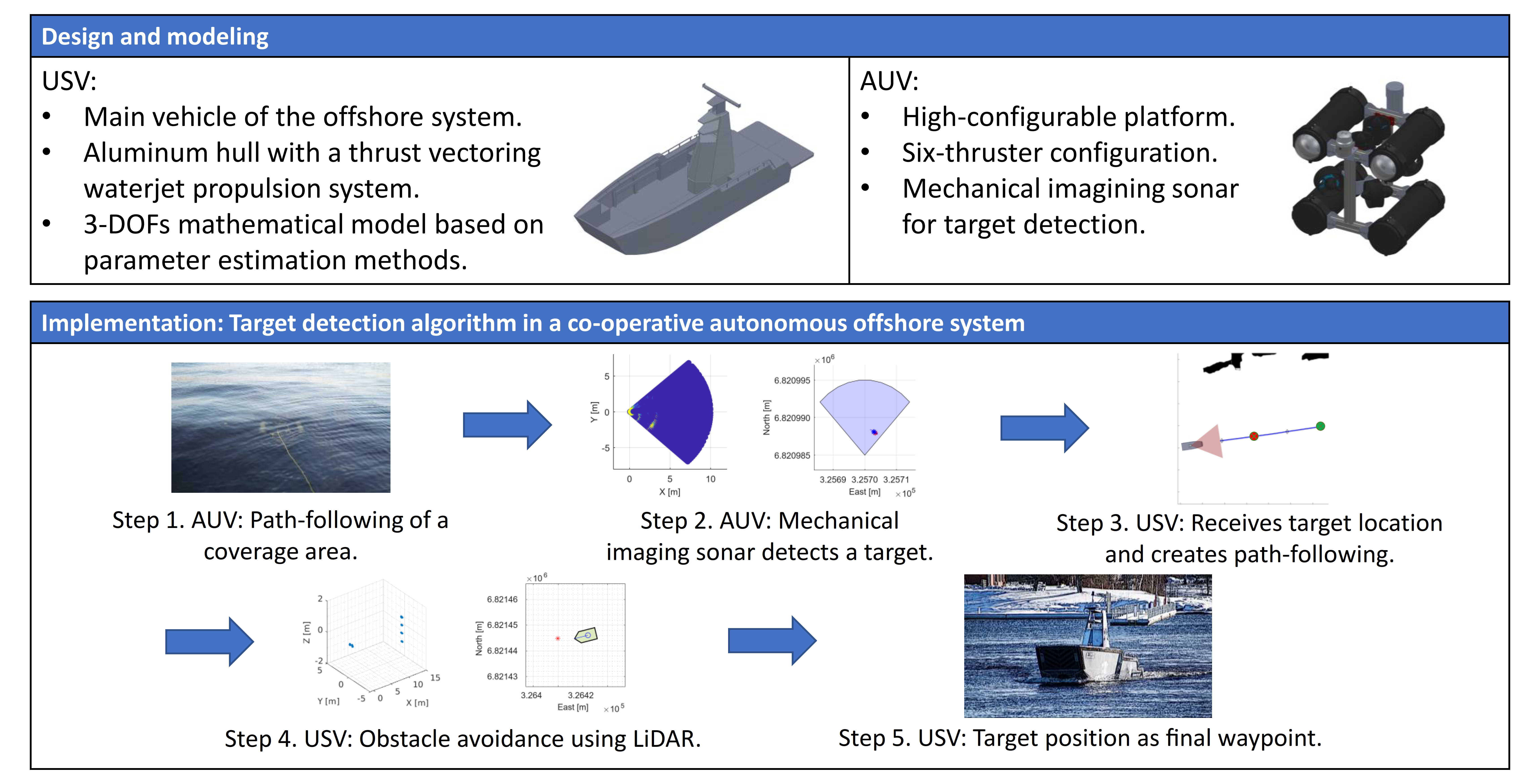
This article uses an under-actuated USV as the primary vehicle in the co-operative autonomous offshore system. The USV is an aluminum hull with a thrust vectoring waterjet propulsion system, which provides optimal maneuverability using a twin waterjet configuration. Figure 1 shows a simplified model of the vehicle, where the port and starboard (STDB) waterjets produce the necessary thrust forces to move forward, backward, sideways or performing turns. Additionally, Figure 1 includes the position and orientation of the USV in the North-East-Down (NED) coordinate system. The NED coordinate system is related to planar Cartesian coordinates, so a coordinate transformation is performed from the GPS-compass output to get the USV’s absolute position. This transformation is between longitude and latitude (l, $\mu$) from the world geodetic system 84 (WGS84) coordinate system and ETRS-TM35FIN [22], which displays the NED position ($x_{\mathrm{USV}}$, $y_{\mathrm{USV}}$). The Euler angles provide the USV heading or yaw angle $\psi$. The motion of the USV has three DOFs, which are surge, sway, and yaw (linear (u, v), and angular r velocities) while ignoring roll, pitch, and heave motions.

2.2. USV Modeling

The development of an adequate maneuvering model will simplify the GNC algorithms design and simulation. The three DOFs horizontal plane model for maneuvering of a USV consists of the rigid-body kinetics [5]

$$\mathit{M}\dot{\mathit{\nu }}+\mathit{C}\left(\mathit{\nu }\right)\mathit{\nu }+\mathit{D}\left(\mathit{\nu }\right)\mathit{\nu }=\mathit{\tau }+{\mathit{\tau }}_{\mathrm{wind}}+{\mathit{\tau }}_{\mathrm{wave}},$$

(1)

where $\mathit{\nu }={\left[u,v,r\right]}^T$ is the velocity vector composed of surge, sway and yaw. $\mathit{\tau }=\left[{\tau }_{\mathrm{u}},0,{\tau }_{\mathrm{r}}\right]$ is the vector forces and moments generated by twin waterjet configuration, while ${\mathit{\tau }}_{\mathrm{wind}}$ and ${\mathit{\tau }}_{\mathrm{wave}}$ are the environmental forces. $\mathit{M}$, $\mathit{C}\left(\mathit{\nu }\right)$, and $\mathit{D}\left(\mathit{\nu }\right)$ are the mass, Coriolis and damping matrices, respectively, where $\mathit{M}$ and $\mathit{C}\left(\mathit{\nu }\right)$ combine added and rigid-body terms. The mass matrix $\mathit{M}$ is defined by

$$\mathit{M}={\mathit{M}}_{\mathrm{RB}}+{\mathit{M}}_{\mathrm{A}}=\left[\begin{array}{ccc}m-X_{\dot{u}}& 0& 0\\ 0& m-Y_{\dot{v}}& m{x}_{\mathrm{g}}-Y_{\dot{r}}\\ 0& m{x}_{\mathrm{g}}-Y_{\dot{r}}& I_{\mathrm{z}}-N_{\dot{r}}\end{array}\right],$$

(2)

where m is the mass of the vehicle, $I_{\mathrm{z}}$ is the moment of inertia about $z_{\mathrm{b}}$ axis, ${\mathit{r}}_{\mathrm{g}}^b$ = ${\left[x_{\mathrm{g}},y_{\mathrm{g}},z_{\mathrm{g}}\right]}^{⊺}$ is the vector from origin $o_{\mathrm{b}}$ to centre of gravity CG, and $X_{\dot{u}}$, $Y_{\dot{v}}$, $Y_{\dot{r}}$, and $N_{\dot{r}}$ represent hydrodynamic added mass. The moment of inertia $I_{\mathrm{z}}$ at the pivot point has been estimated based on the calculation of the moments of inertia in the rear $I_{\mathrm{z},\mathrm{rear}}$ and front $I_{\mathrm{z},\mathrm{front}}$ of the USV. These moments of inertia are defined by

$$I_{\mathrm{z},\mathrm{rear}}=m_{\mathrm{pt}}{l}_{\mathrm{pt}}^2+\left(\frac{1}{3}{m}_{\mathrm{hull}}{c}_{\mathrm{g}}\right)l_{\mathrm{pivot}}^2,$$

(3)

$$I_{\mathrm{z},\mathrm{front}}=\frac{1}{3}{m}_{\mathrm{hull}}\left(1-c_{\mathrm{g}}\right) \kappa {\left(l_{\mathrm{USV}}-l_{\mathrm{pivot}}\right)}^2,$$

(4)

where $m_{\mathrm{pt}}$ is the estimated powertrain mass (engines, waterjets, fuel, etc.), $l_{\mathrm{pt}}$ is the estimated location of the powertrain mass, $m_{\mathrm{hull}}$ is the hull weight without powertrain mass, $c_{\mathrm{g}}$ is the relative center of mass point having one as the front of the USV, $l_{\mathrm{pivot}}$ is the pivot point location, $\kappa$ is a scaling factor as the mass is not evenly distributed from the pivot point to the front of the USV, and $l_{\mathrm{USV}}$ is the length of the USV. The total moment of inertia $I_{\mathrm{z}}$ is defined by

$$I_{\mathrm{z}}=\left(I_{\mathrm{z},\mathrm{rear}}+I_{\mathrm{z},\mathrm{front}}\right)I_{\mathrm{cor}},$$

(5)

where $I_{\mathrm{cor}}$ is the tuning factor for the moment of inertia.

The Coriolis-centripetal matrix $\mathit{C}\left(\mathit{\nu }\right)$ can always be parameterized such that $\mathit{C}\left(\mathit{\nu }\right)$ = ${\mathit{C}}^{⊺}\left(\mathit{\nu }\right)$ [23]. However, linearization of the Coriolis and centripetal forces ${\mathit{C}}_{\mathrm{RB}}\left(\mathit{\nu }\right)$ and ${\mathit{C}}_{\mathrm{A}}\left(\mathit{\nu }\right)$ about zero angular velocity $\left(p=q=r=0\right)$ implies that the Coriolis and centripetal terms can be removed from the above expressions, that is ${\mathit{C}}_{\mathrm{RB}}\left(\mathit{\nu }\right)$ = ${\mathit{C}}_{\mathrm{A}}\left(\mathit{\nu }\right)$ = 0 [24]. Additionally, the mathematical model is simplified to take into account only surge and yaw motions, so Coriolis and centripetal terms have been removed at the three DOFs dynamic model in this study.

The different damping terms contribute to linear and quadratic damping [5]. Nonetheless, it is generally difficult to distinguish these effects. The total hydrodynamic damping matrix $\mathit{D}\left({\mathit{\nu }}_r\right)$ is the sum of the linear part ${\mathit{D}}_{\mathrm{lin}}$ and the nonlinear part ${\mathit{D}}_{\mathrm{nlin}}\left({\mathit{\nu }}_r\right)$ such that

$$\mathit{D}\left({\mathit{\nu }}_r\right)={\mathit{D}}_{\mathrm{lin}}+{\mathit{D}}_{\mathrm{nlin}}\left({\mathit{\nu }}_r\right),$$

(6)

where ${\mathit{D}}_{\mathrm{lin}}$ is the linear damping matrix produced by potential damping and possible skin friction, and ${\mathit{D}}_{\mathrm{nlin}}\left({\mathit{\nu }}_r\right)$ is the nonlinear damping matrix as a result of the quadratic damping and higher-order terms, defined by

$${\mathit{D}}_{\mathrm{lin}}=\left[\begin{array}{ccc}-X_u& 0& 0\\ 0& -Y_v& -Y_r\\ 0& -Y_r& -N_r\end{array}\right],$$

(7)

$${\mathit{D}}_{\mathrm{nlin}}\left({\mathit{\nu }}_r\right)=\left[\begin{array}{ccc}-X_{\left|u\right|u}& 0& 0\\ 0& -Y_{\left|v\right|v}& 0\\ 0& 0& -N_{\left|r\right|r}\end{array}\right]\left|{\mathit{\nu }}_r\right|.$$

(8)

The USV used in this study includes the AJ245 waterjet units [25]. The nozzle position $P_{\mathrm{nozzle}}$ varies the direction of the jet flow, which generates the force needed for turning. Thus, the total thrust force $F_{\mathrm{total}}$ combines the engine rpm of the waterjet $n_{\mathrm{rpm}}$ and $P_{\mathrm{nozzle}}$. The variable $n_{\mathrm{rpm}}$ is directly gathered from the waterjet engine, and $P_{\mathrm{nozzle}}$ is a variable from −10,000 to 10,000, with 0 as the neutral position and equal to forward motion.

Table 1. Data obtained from manufacturer for an operating point of a single AJ245 waterjet unit.

Surge Speed [kt]	Thrust Force [kN]
2	2
4	1.85
6	1.7

shows the data obtained from the manufacturer Alamarin-Jet Oy for these waterjet units at a specific operating point. This operating point is selected at 1800 rpm, nozzle in the neutral position, and bucket in the full up position.

The thrust forces and torques for the mathematical model of the USV are defined according to the manufacturer’s data and an affinity law. Thus, a two-dimensional (2D) lookup table can include the relation between the shaft rotational speed of the waterjet engine N with the thrust force per waterjet F. The affinity law used to obtain the thrust force at the waterjet units is defined by

$$\frac{F_1}{F_2}={\left(\frac{N_1}{N_2}\right)}^2.$$

(9)

Figure 2 shows the results for the affinity law with the manufacturer’s data for a waterjet engine from 600 to 2400 rpm, which match the operational engine speeds of this study.

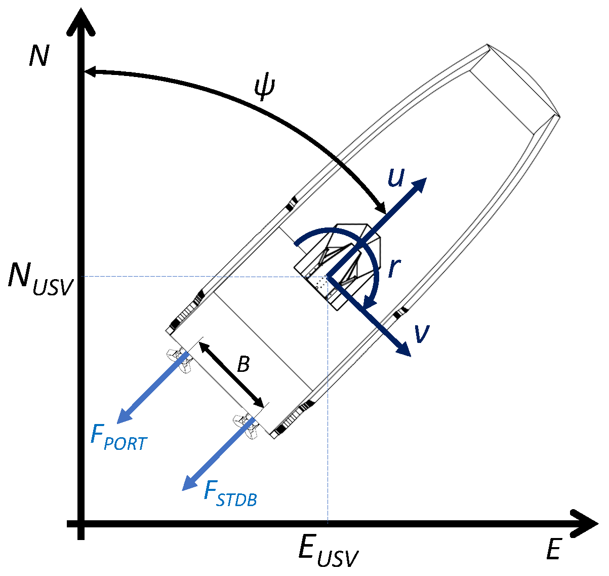
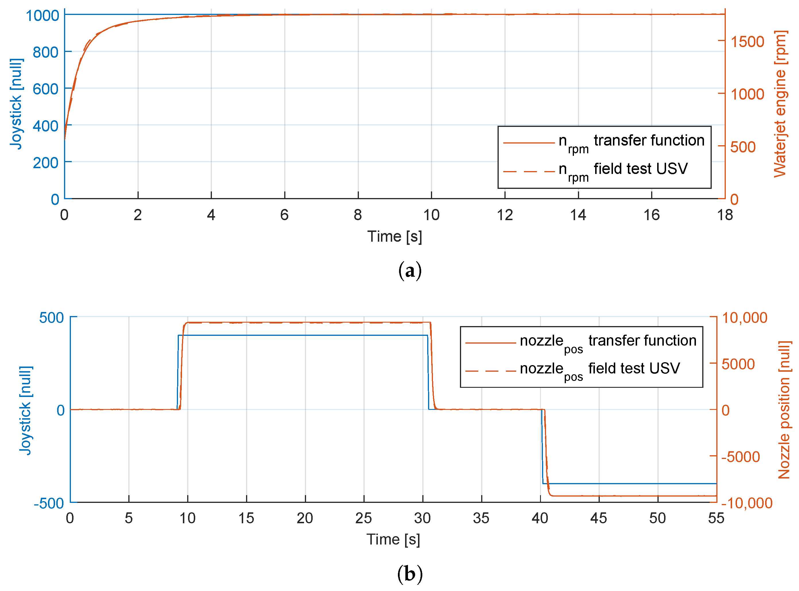
In the mathematical model, a 2D lookup table provides the engine rpm and the surge speed of the USV as inputs, and the total thrust generated by the waterjet unit as output. Also, a one-dimensional (1D) lookup table $f\left(Jo{y}_u\right)$ obtains the engine rpm depending on the joystick input for surge motion, and a second-order transfer function adds the waterjet dynamics of the engine rpm into the mathematical model. This transfer function is obtained using the SI tool from MATLAB and the field test data of the USV. Thus, the engine rpm is calculated based on the combination of the 1D lookup table and the engine rpm transfer function, defined by

$$n_{\mathrm{rpm}}\left(s\right)=\frac{0.317s^2+2.793s+1.828}{s^2+3.499s+1.828}f\left(Jo{y}_u\right).$$

(10)

In the case of the heading motion of the USV, the total efficiency ${\eta }_{\mathrm{nozzle}}$ for the thrust force depends on the nozzle position (which refers to the angle of the waterjet thrust force ${\alpha }_{\mathrm{nozzle}}$). According to the waterjet manufacturer, if the nozzle position is deviated to a maximum nozzle angle ${\eta }_{\mathrm{nozzle}}$ = ±25° (related to $P_{\mathrm{nozzle}}$ = ±10,000), efficiency drops exponentially to 30–40% of the maximum (center). The exponential function is obtained using the general exponential model.

$${\eta }_{\mathrm{nozzle}}\left(P_{\mathrm{nozzle}}\right)=aexp\left(b{P}_{\mathrm{nozzle}}\right),$$

(11)

where $a=1$ and $b=-9.163\times {10}^{-5}$.

Similarly to the dynamics of the waterjet calculation for the engine rpm, the nozzle position includes a 1D lookup table $f\left(Jo{y}_r\right)$ and a first-order transfer function. This transfer function is obtained also from the SI tool from MATLAB based on field test data. The nozzle position of each waterjet is defined by

$$P_{\mathrm{nozzle}}\left(s\right)=\frac{-exp(-0.25s)}{0.1s+1}f\left(Jo{y}_r\right).$$

(12)

Regarding the behavior of the second-order transfer functions for both engine rpm and nozzle position, Figure 3 shows the comparison between the SI tool transfer function and field test data for both $n_{\mathrm{rpm}}$ and $P_{\mathrm{nozzle}}$ variables.

Additionally, the parameters for the 1D Lookup table are obtained from field test data and are presented in

Table 2. 1D Lookup Table parameters.

$Jo{y}_u$	400	500	600	700	800	900	1000
$n_{\mathrm{rpm}}$	690	920	1110	1300	1480	1650	1820
$Jo{y}_r$	0	50	150	200	250	300	400
$P_{\mathrm{nozzle}}$	0	1175	3500	4665	5830	7000	9325

.

Finally, the vector $\mathit{\tau }=\left[{\tau }_{\mathrm{u}},0,{\tau }_{\mathrm{r}}\right]$, which represents the forces and moments generated by the two waterjets, is defined by

$$\left\{\begin{array}{c}{\tau }_{\mathrm{u}}=(F_{\mathrm{PORT}}+F_{\mathrm{STDB}}){\eta }_{\mathrm{nozzle}}\hfill \\ {\tau }_{\mathrm{r}}=l_{\mathrm{pivot}}sin\left({\alpha }_{\mathrm{nozzle}}\right)(F_{\mathrm{PORT}}+F_{\mathrm{STDB}}){\eta }_{\mathrm{nozzle}}\hfill \end{array}\right..$$

(13)

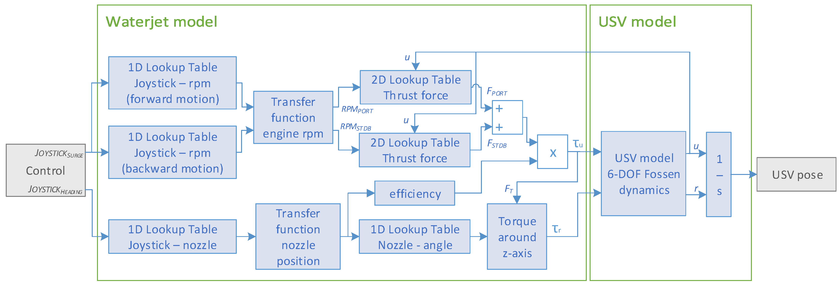
Figure 4 shows the schematic with all the necessary functions for the USV dynamic model, from the joystick controller input to the vehicle’s position output. The waterjet model includes the 1D lookup table to translate between joystick commands to rpm, the second-order transfer function, and the 2D lookup table related to the thrust force of each waterjet unit. Furthermore, it also includes the 1D lookup table to translate between joystick commands to the nozzle position, the first-order transfer function, the thrust force efficiency depending on the nozzle position, and the calculation of the total torque. Both thrust force ${\tau }_{\mathrm{u}}$ and torque ${\tau }_{\mathrm{r}}$ are the inputs in the mathematical model of the USV based on the three DOFs dynamic model. The position and orientation of the USV are performed by integrating the velocity vector $\mathit{\nu }$.

2.3. USV Model-Validation Using Parameter Estimation

The matrices $\mathit{M}$ and $\mathit{D}\left(\mathit{\nu }\right)$ of the three DOFs Dynamic model are estimated with the parameter estimation tool from MATLAB-Simulink. The matrices are defined in the Simulink model by creating the matrices from input values. Then, the MATLAB-Simulink tool can estimate the individual coefficients of the dynamic matrices.

There are two different parameter estimation runs related to surge and yaw motion.

Table 3. Principal characteristics of the under-actuated USV.

Parameter	Value
m	3500 $\left[\mathrm{kg}\right]$
$m_{\mathrm{pt}}$	1100 $\left[\mathrm{kg}\right]$
$m_{\mathrm{hull}}$	2400 $\left[\mathrm{kg}\right]$
$l_{\mathrm{USV}}$	8 $\left[\mathrm{m}\right]$
$l_{\mathrm{pivot}}$	2.40 $\left[\mathrm{m}\right]$
$l_{\mathrm{pt}}$	2.16 $\left[\mathrm{m}\right]$
$\kappa$	0.70
$c_{\mathrm{g}}$	0.30
$I_{\mathrm{cor}}$	0.6
$I_{\mathrm{z}}$ from (5)	11,284.61 $\left[\mathrm{kg}{\mathrm{m}}^2\right]$
$x_{\mathrm{g}}$	0.0425 $\left[\mathrm{m}\right]$

shows the constant values shared in both experiments, while

Table 4. Parameter estimation results for the surge and yaw motion coefficients.

Parameter	Value
$X_u$	−10.586
$X_{\dot{u}}$	−3277
$X_{\left|u\right|u}$	315.45
$N_r$	3907.9
$N_{\dot{r}}$	−36.555
$N_{\left|r\right|r}$	3459.6

shows the coefficients obtained from the parameter estimation tool with their results. Only surge and yaw motion coefficients, $X_u$, $X_{\dot{u}}$, $X_{\left|u\right|u}$ and $N_r$, $N_{\dot{r}}$, $N_{\left|r\right|r}$ respectively, have been considered and estimated in this study, as the mathematical model focuses in these two USV motions.

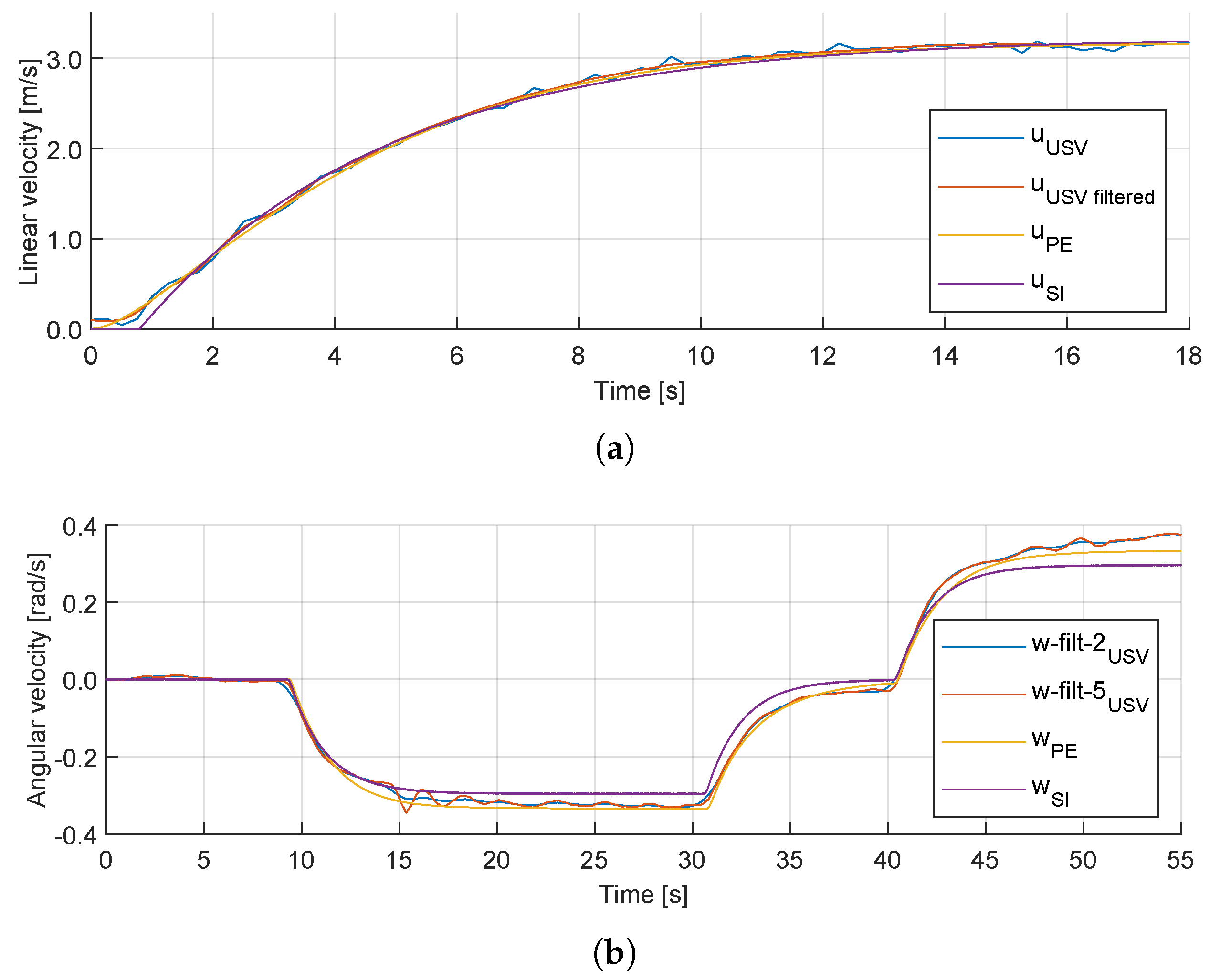
Figure 5 shows the comparison between the field tests, which include raw and filtered USV linear and angular velocity, the three DOFs dynamic model with the coefficients obtained from the parameter estimation, and the SI results from [10], for the joystick controller input shown in Figure 3. As shown in both linear and angular velocities results, the parameter estimation results improve the previous SI approach, giving an accurate output of the USV maneuvering compared to the field test results.

2.4. Overview of the AUV

This article uses a high configurable AUV platform for different scientific instrumentation. This vehicle contains basic instrumentation and sensors for localization and target detection, including a USBL and a depth sensor for underwater localization and navigation, an AHRS from the flight control for the navigation of the AUV, and a mechanical imaging sonar (Tritech Micron [26]) as main underwater perception sensor.

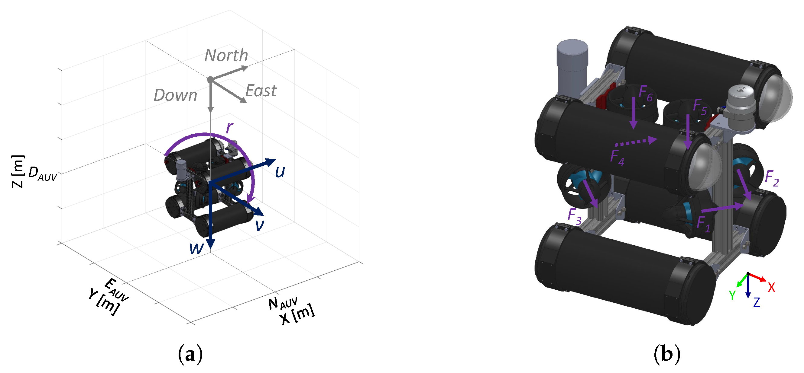
Figure 6a shows a simplified model of the AUV. This AUV uses a six-thruster configuration to provide thrust forces when moving in the surge, sway, heave motions, or performing turns. Also, the position and velocities of the AUV are illustrated in Figure 6a. The general AUV motion in six DOFs is modeled by using the NED local coordinate system. AUV position and velocities are considered with the following vectors

$$\mathit{\eta }={\left[N,E,D,\varphi ,\theta ,\psi \right]}^{\top },\mathit{\nu }={\left[u,v,w,p,q,r\right]}^{\top },$$

(14)

where $N,E,D$ denote the NED positions in Earth-fixed coordinates, $\varphi ,\theta ,\psi$ are the Euler angles, $u,v,w$ are the body-fixed linear velocities, and $p,q,r$ are the body-fixed angular velocities [5].

The design and modeling of the AUV should be studied using a theoretical six DOFs dynamic model [27]. However, due to the lack of instrumentation, it is not possible to obtain accurate navigation data. Thus, the AUV is not fully simulated, and just simple control commands are established for navigation. Once that navigation data is available, it is possible to use the same approach as the USV mathematical model to obtain the six DOFs dynamic model, using the parameter estimation or SI tools based on field test data. Regarding the control of the AUV, thrusters are located as it is shown in Figure 6b, where thrusters $T_1$, $T_2$, $T_3$, and $T_4$ effects in surge, sway, and yawing, and thrusters $T_5$ and $T_6$ effects in heave and rolling motions.

3. Gnc System for the Co-Operative Tasks

This study has the target detection and the guidance algorithms as main modules of the GNC architecture of the offshore multi-vehicle system. This section describes both of these algorithms for each platform and the description of the multi-vehicle guidance system.

3.1. Target Detection System

The mechanical imaging sonar installed at the AUV and the LiDAR at the USV are the primary perception sensors in the co-operative autonomous offshore system. The target detection algorithm includes the application in both perception sensors, depending on the position of the objects (underwater or over the water surface).

For the mechanical imaging sonar, the employed algorithm consists of analyzing the acoustic intensity at every bin to determine the presence of an underwater vehicle. The Tritech Micron sonar [26] has an operating frequency chirp centered on 700 kHz, a beamwidth of 35° vertical and 3° horizontal, a range from 0.3 to 75 m, a range resolution of approximately 7.5 mm, and a configurable mechanical resolution of 0.45°, 0.9°, 1.8°, and 3.6°. In this study, the maximum range used to detect an obstacle is 10 m, a forward field-of-view (FoV) of 90°, and a mechanical resolution of 1.8°. If the target is known a priori to be narrow, the imaging sonar can be configured with a lower resolution to detect the object.

Regarding the data obtained from the mechanical imaging sonar, it contains the heading of the beam ${\theta }_{\mathrm{scan}}$, the location of the specific point in Cartesian coordinates $P_{\mathrm{scan}}$, and the intensity at every bin $I_{\mathrm{scan}}$. The dynamic range of the mechanical imaging sonar is 80 dB. Then, the dynamic range controls allow to adjust the position of a sampling window within the defined dynamic band range of the received signal, and it translates the intensity at every bin to an integer value ranging between 0 and 255.

After data acquisition from the mechanical imaging sonar, Algorithm 1 shows the post-processing steps for target detection. This algorithm includes the position of the highest intensity value for each bin in polar coordinates, filtering the data in the range of [0,1.5] meters to avoid possible noise from the AUV structure.

Algorithm 1: Post-processing of the mechanical imaging sonar data for target detection.

Algorithm 1 provides the post-processing of a single bin of a specific angle. An additional function forms an array of number of scans $n_{\mathrm{scans}}$, obtained from ${\theta }_{\mathrm{scan},\min }$, ${\theta }_{\mathrm{scan},\max }$, and ${\theta }_{\mathrm{scan},\mathrm{increment}}$ parameters of the mechanical imaging sonar to create the complete array of scans from the sonar. After gathering the scan array, the position of the targets needs to be calculated. The data from the perception sensors is obtained in the body-fixed reference frame (BODY), and it requires a translation into an absolute coordinate system. This translation is defined by

$$\left[\begin{array}{c}{x}_{\mathrm{obs}}\\ y_{\mathrm{obs}}\end{array}\right]={\mathit{R}}_{\mathit{z}}\left({\psi }_{\mathrm{AV}}\right)\left[\begin{array}{c}{x}_{\mathrm{scan}}\\ y_{\mathrm{scan}}\end{array}\right],$$

(15)

where ${\mathit{R}}_{\mathit{z}}\left({\psi }_{\mathrm{AV}}\right)$ is the rotation matrix around the z-axis using the heading angle ${\psi }_{\mathrm{AV}}$ of the selected AV. This rotation matrix translates between the BODY and the East-North-Up (ENU) coordinate system. The rotation matrix ${\mathit{R}}_{\mathit{z}}\left({\psi }_{\mathrm{AV}}\right)$ in 2D is defined by

$${\mathit{R}}_{\mathit{z}}\left({\psi }_{\mathrm{AV}}\right)=\left[\begin{array}{cc}cos\left({\psi }_{\mathrm{AV}}\right)& sin\left({\psi }_{\mathrm{AV}}\right)\\ -sin\left({\psi }_{\mathrm{AV}}\right)& cos\left({\psi }_{\mathrm{AV}}\right)\end{array}\right].$$

(16)

After locating the obstacle by the mechanical imaging sonar in the ENU coordinate system, the target’s origin position ($N_{\mathrm{o}},E_{\mathrm{o}}$) is defined by

$$\left[\begin{array}{c}{N}_{\mathrm{o}}\\ E_{\mathrm{o}}\end{array}\right]=\left[\begin{array}{c}{N}_{\mathrm{AV}}\\ E_{\mathrm{AV}}\end{array}\right] + {\mathit{R}}_{\mathit{x}}\left(\gamma \right)\left[\begin{array}{c}\frac{x_{\mathrm{obs},\mathrm{init}}+x_{\mathrm{obs},\mathrm{end}}}{2}\\ \frac{y_{\mathrm{obs},\mathrm{init}}+y_{\mathrm{obs},\mathrm{end}}}{2}\end{array}\right],$$

(17)

where ${\mathit{R}}_{\mathit{x}}\left(\gamma \right)$ is the rotation matrix around x-axis with $\gamma =pi\left[\mathrm{rad}\right]$. This matrix is used to translate between ENU to NED coordinate system used for the offshore navigation. The ${\mathit{R}}_{\mathit{x}}\left(\gamma \right)$ rotation matrix in 2D is defined by

$${\mathit{R}}_{\mathit{x}}\left(\gamma \right)=\left[\begin{array}{cc}1& 0\\ 0& cos\left(\gamma \right)\end{array}\right].$$

(18)

Algorithm 2 includes the detected target localization for the perception sensor data array. This algorithm distinguishes between different targets depending on the consecutive elements in the data array, and the origin position of the targets is sent to the GNC algorithm to proceed with the autonomous navigation of the offshore system.

Algorithm 2: Localization of the detected targets.

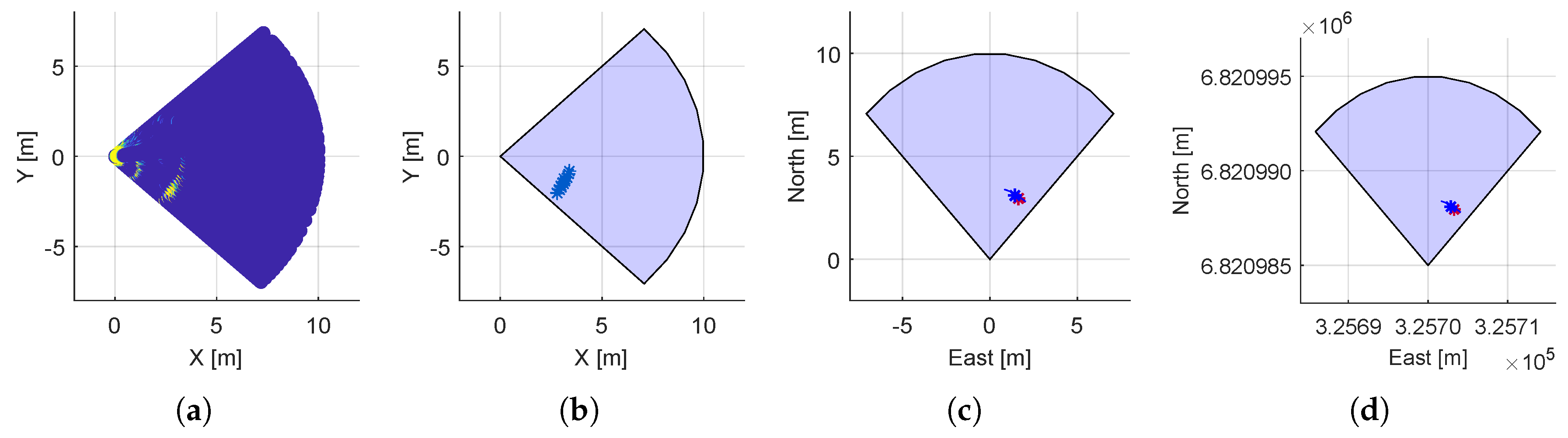
Figure 7 shows the steps from the scan data obtained from the mechanical imaging sonar in the BODY reference frame to the final origin position of the detected targets. Figure 7a shows the raw data from the mechanical imaging sonar. Then, Figure 7b shows the post-processing described in Algorithm 1. Finally, Figure 7c,d represents the origin position of the targets in NED coordinate system, with relative to origin [0,0] and absolute coordinates respectively.

Regarding the USV platform, the SICK MRS1000 LiDAR [28] is the primary perception sensor. This LiDAR has four spread-out scan planes and a multi-echo analysis to be used in harsh environment applications, as it can avoid the noise produced by fog, rain, or dust. Also, this device has a 275° aperture angle, and a working range from 0.2 to 64 m. Thus, in case that the target is above the water surface, it can be detected by the LiDAR sensor.

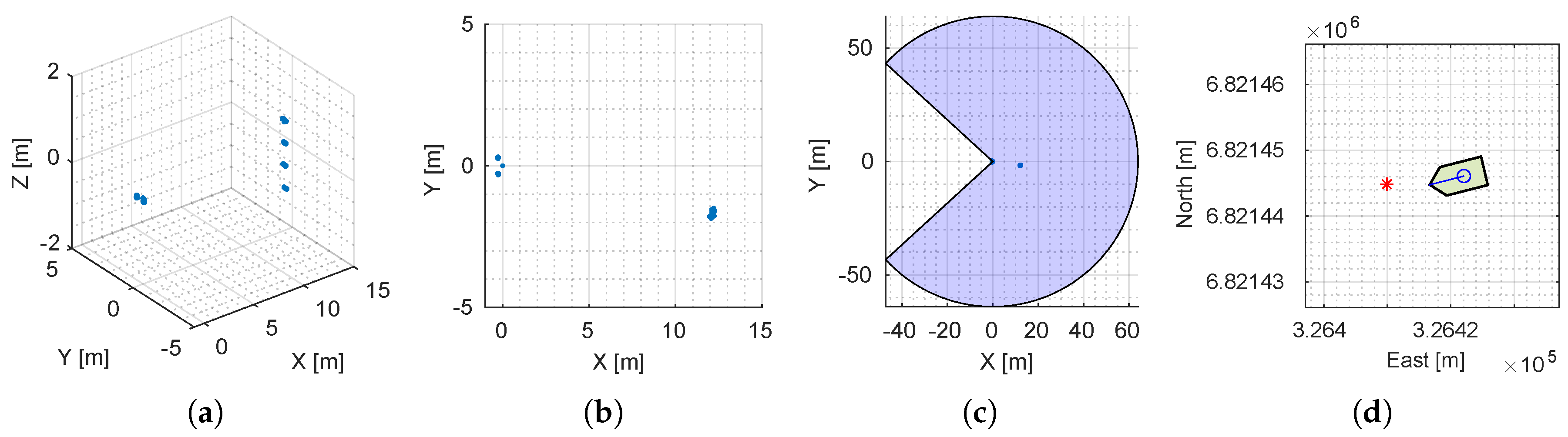
The algorithm for target detection is similar to the described for the mechanical imaging sonar. The only difference is that the LiDAR contains four spread-out scan planes, acquiring three-dimensional (3D) scan data (see Figure 8a). The target detection algorithm is simplified by translating the received data to 2D by avoiding the z-axis from the sensor data (see Figure 8b). Figure 8c shows the maximum detection range and aperture angle with the scan data in the BODY reference frame. Finally, Figure 8d shows the origin’s position of the targets in the NED coordinate system after applying Algorithm 2.

The same procedure detects obstacles from the LiDAR for the path-following with the obstacle avoidance algorithm. After obtaining the origin position [$N_{\mathrm{o}}$, $E_{\mathrm{o}}$] from Algorithm 2, the obstacle avoidance algorithm can define a safety boundary box around the obstacle [10].

3.2. Guidance System for Multi-Vehicle System

The multi-vehicle system aims firstly to detect a target using the AUV in a specific offshore area, and after that, sends the location to the USV to do further exploration of the target. Thus, a path-following algorithm is essential for both AUV and USV subsystems. This algorithm intends to reach every waypoint of a specific path independent of time. A commonly used method for path-following is the named LOS guidance, which is chosen as a reference trajectory in this study.

3.2.1. Auv Guidance System

The heading control can use a LOS vector from the AUV position to the next waypoint, similar to [5]. The LOS path-following controller used in this study is the same as the one defined in [10]. However, the AUV movement includes a heave motion, which is avoided by keeping a constant depth for the path-following algorithm. This controller computes the course angle ${\psi }_{\mathrm{d}}$ based on the path-tangential angle ${\chi }_{\mathrm{p}}$ and the velocity-path relative angle ${\chi }_{\mathrm{r}}$. The lookahead-based steering can be implemented related to the heading controller applying the transformation defined as

$${\psi }_{\mathrm{d}}={\chi }_{\mathrm{p}}+{\chi }_{\mathrm{r}}-\beta ,$$

(19)

where the variable sideslip (drift) angle $\beta$ [5] has been omitted in this study to simplify the steering law. The velocity-path relative angle ${\chi }_{\mathrm{r}}$ establishes that the velocity has the direction facing a path location that is in a lookahead distance $\Delta \left(t\right)>0$ along of the direct projection [29]. The path-tangential angle ${\chi }_{\mathrm{p}}$ and the velocity-path relative angle ${\chi }_{\mathrm{r}}$ are defined as

$${\chi }_{\mathrm{p}}=atan2(E_{k+1}-E_k,N_{k+1}-N_k),$$

(20)

$${\chi }_{\mathrm{r}}\left(e\right)=arctan(-K_{\mathrm{P}}e-K_{\mathrm{I}}{\int }_0^{t}e\left(\tau \right)d\tau ),$$

(21)

where ($N_k,E_k$) and ($N_{k+1},E_{k+1}$) are the positions of the passed and next waypoint, respectively, the proportional gain is $K_{\mathrm{P}}=1/\Delta \left(t\right)>0$, and $K_{\mathrm{I}}>0$ represents the integral gain. The cross-track error $e\left(t\right)$ is given by

$$e\left(t\right)=-[N_{\mathrm{AUV}}\left(t\right)-N_k]sin\left({\chi }_{\mathrm{p}}\right)+[E_{\mathrm{AUV}}\left(t\right)-E_k]cos\left({\chi }_{\mathrm{p}}\right).$$

(22)

The switching mechanism is declared as a sphere of acceptance for AUVs [30]. This mechanism selects the next waypoint as a lookahead point if the AUV position lies within a sphere with a radius R around the position ($N_{k+1},E_{k+1},D_{k+1}$). The sphere of acceptance is defined as

$${[N_{k+1}-N\left(t\right)]}^2+{[E_{k+1}-E\left(t\right)]}^2+{[D_{k+1}-D\left(t\right)]}^2\le R_{k+1}^2,$$

(23)

where, if the time AUV position ($N\left(t\right),E\left(t\right),D\left(t\right)$) satisfies Equation (23), the next waypoint ($N_{k+1},E_{k+1},D_{k+1}$) needs to be selected. Radius R is equal to three AUV lengths $L_{\mathrm{AUV}}$ ($R=3L_{\mathrm{AUV}}$), as the position is only obtained from the USBL system.

After obtaining the course angle from the LOS path-following algorithm, this algorithm sends the heading commands to the yaw controller to match the aimed path. The main control system of the AUV is formed by three separate PID controllers for surge, heave, and yaw motions. Apart from the heading controller, the heave controller keeps the AUV at a constant depth. Their PID parameters for heading controller are obtained by using rapid control prototyping based on the Ziegler-Nichols PID tuning [31] during field tests. Both amplitude $K_{\mathrm{zn}}$ and period $T_{\mathrm{zn}}$ are calculated for the AUV at the water tank, and then, the PID parameters are defined based on

Table 5. PID parameters for AUV.

Controller	${\mathit{T}}_{\mathbf{zn}}$$\left[\mathbf{s}\right]$	${\mathit{K}}_{\mathbf{zn}}$	${\mathit{K}}_{\mathbf{P}}$	${\mathit{K}}_{\mathbf{I}}$	${\mathit{K}}_{\mathbf{D}}$
Yaw	2.10	5.80	0.580	0.276	0.812
Heave	-	-	300	0.0	0.0
LOS	-	-	0.333	0.0	0.0

. Furthermore, a simple proportional controller has been selected in the heave controller. The surge motion is implemented as a constant PWM value to the thrusters.

3.2.2. USV Guidance System

Same as the AUV guidance system, USV heading control uses a LOS vector from the USV position to the next waypoint. The LOS path-following controller used in this study is the same as the one defined in [10], including the obstacle avoidance capabilities with the safety boundary box approach. The LOS path-following controller of the USV uses the same path-tangential angle ${\chi }_{\mathrm{p}}$ defined in Equation (20), the velocity-path relative angle defined in Equation (21), and the total lookahead-based steering from Equation (19). The switching mechanism is selected as a circle of acceptance for surface vehicles [5]. It selects the next waypoint as a lookahead point if the position of the USV lies within a circle with radius R around ($N_{k+1},E_{k+1}$). This circle of acceptance is defined as

$${[N_{\mathrm{USV}}\left(t\right)-N_{k+1}]}^2+{[E_{\mathrm{USV}}\left(t\right)-E_{k+1}]}^2\le R_{k+1}^2,$$

(24)

where, if the time surface vehicle position ($N_{\mathrm{USV}}\left(t\right),E_{\mathrm{USV}}\left(t\right)$) satisfies (24), the next waypoint ($N_{k+1},E_{k+1}$) needs to be selected. Radius R is equal to two USV lengths $L_{\mathrm{USV}}$ ($R=2L_{\mathrm{USV}}$).

3.2.3. Multi-Vehicle Guidance System

At the beginning of the control scenario, the USV keeps its position in dynamic positioning (DP) mode while the AUV is trying to search for targets in the coverage area. A DP vessel is a vessel that maintains its position exclusively using active thrusters [24]. This study considers the use of conventional controllers with cascade with low-pass and notch filters to simplify the implementation. The control problem is solved by using PID-controllers for surge, sway, and yaw motions.

The AUV in this study aims to detect a target in a specific offshore area. The coverage area is defined as a set of waypoints to cover a far-reaching range inside. However, this coverage area has been substituted by a straight-path to simplify the control scenario. After detecting the object by the target detection system, it sends a stop command to the AUV, and the vehicle stays in its position until it received further instructions from the USV. As the AUV does not contain enough instrumentation to have a precise localization of the subsystem, the AUV in this study stops its thrusters instead of having a DP control of its final position. Additionally, if the target detection algorithm does not recognize any target in the coverage area, the AUV stops after reaching the last waypoint of the predefined path.

After receiving the target position by the USV, the path-following algorithm creates the waypoints with a straight-line trajectory. The first waypoint matches the current position of the USV at the time that the target position is received, and the last waypoint is the target position itself. With a constant distance between waypoints of 10 m, the number of waypoints is related to the length of the straight-line path. These waypoints are sent to the LOS path-following algorithm to calculate the course angle of the USV. Furthermore, an additional switching mechanism is included using the same principle as the circle of acceptance defined in (24) to stop the LOS path-following controller once the USV has reached the last waypoint of the predefined path. Then, the guidance system does not send any heading or surge commands to the controllers, and there is no output from the target detection algorithm. In this case, the USV changes to DP internal algorithm keeping its position constant.

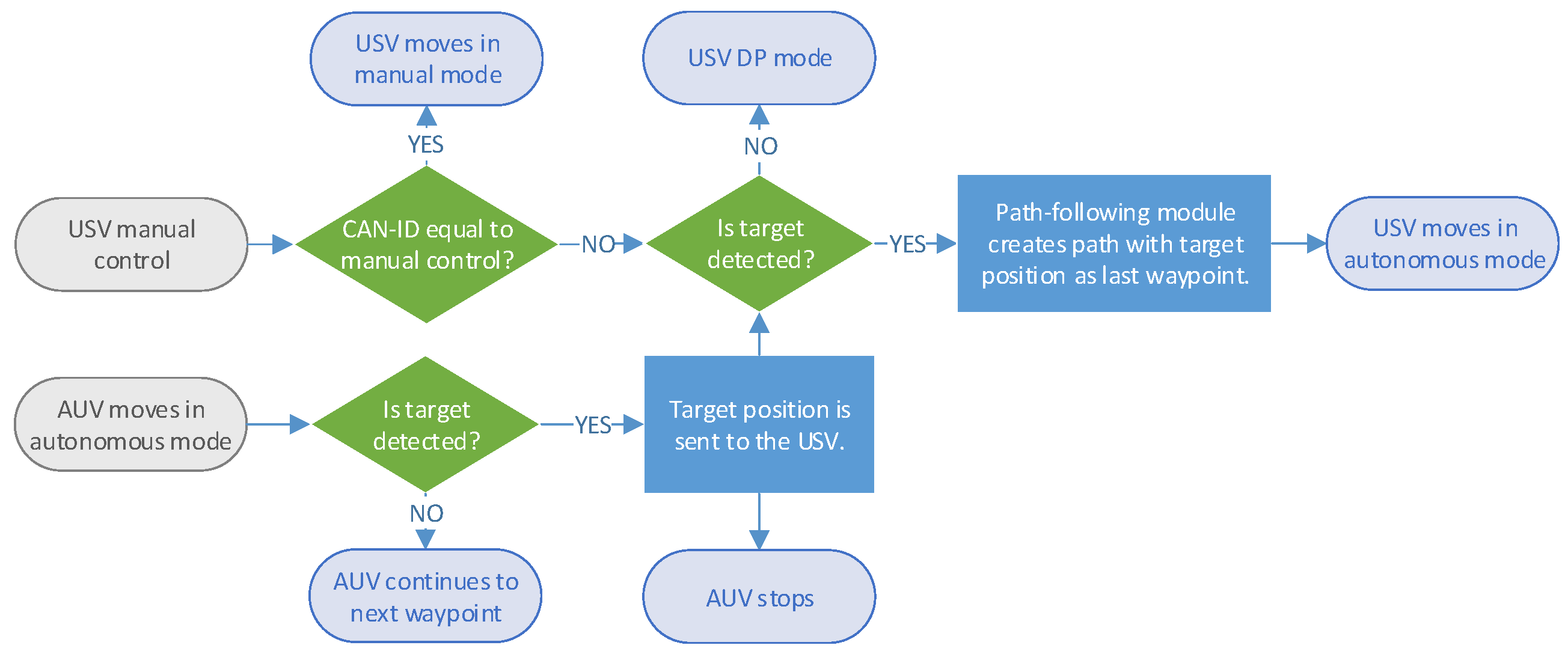
Figure 9 shows the priority control level for the multi-vehicle guidance system. First, the AUV starts the path-following of the coverage area based on predefined waypoints. The vehicle continues to the next waypoint until the mechanical imaging sonar detects a target. Then, the AUV stops its operation, and the target position is transmitted to the USV. The USV keeps its position in DP mode and, when the target position is received, it starts the path-following with obstacle avoidance operation with the target position as the final waypoint of the USV trajectory. After reaching the last waypoint, the USV stops and uses the DP mode to keep its position, allowing the GCS to have further inspection of the detected target. Additionally, the steering wheel and 3-axis joystick, both forming the manual control of the USV, provides the safety feature in the autonomous algorithm.

4. Experimental Validation

4.1. System Implementation

For this particular study, the USV and AUV platforms incorporate multiple mechatronic systems to implement the target detection algorithm. Both vehicles include high-level control (computers with ROS), which performs complex computations and processes the data obtained from localization and perception sensors, and low-level control (sensors and actuators units), that runs as the basic interface for vehicle operations. Also, an intermediate-level (or mid-level) control is included, which is the main link between low-level data acquisition and high-level logic operations.

Figure 10 shows the mechatronic systems used in the USV, including also the connection to the AUV and external MATLAB-Simulink computer through the main network switch. These devices are the link to the co-operative autonomous offshore system. In general, the USV platform is equipped with a payload for navigation (high precision GPS-Compass), LiDAR as the main perception sensor, SeaTrac acoustic system for USBL localization, and communication with the AUV, and WiFi for communication with the GCS. The USV system implementation is the same as the one studied in [10]. For the high-level control, the ROS master includes the necessary stand-alone ROS-nodes for the path-following with obstacle avoidance. The display computers act as intermediate-level control for translation between CAN bus and ROS messages. Also, they are in charge of sending joystick commands to the waterjet control units based upon priority levels.

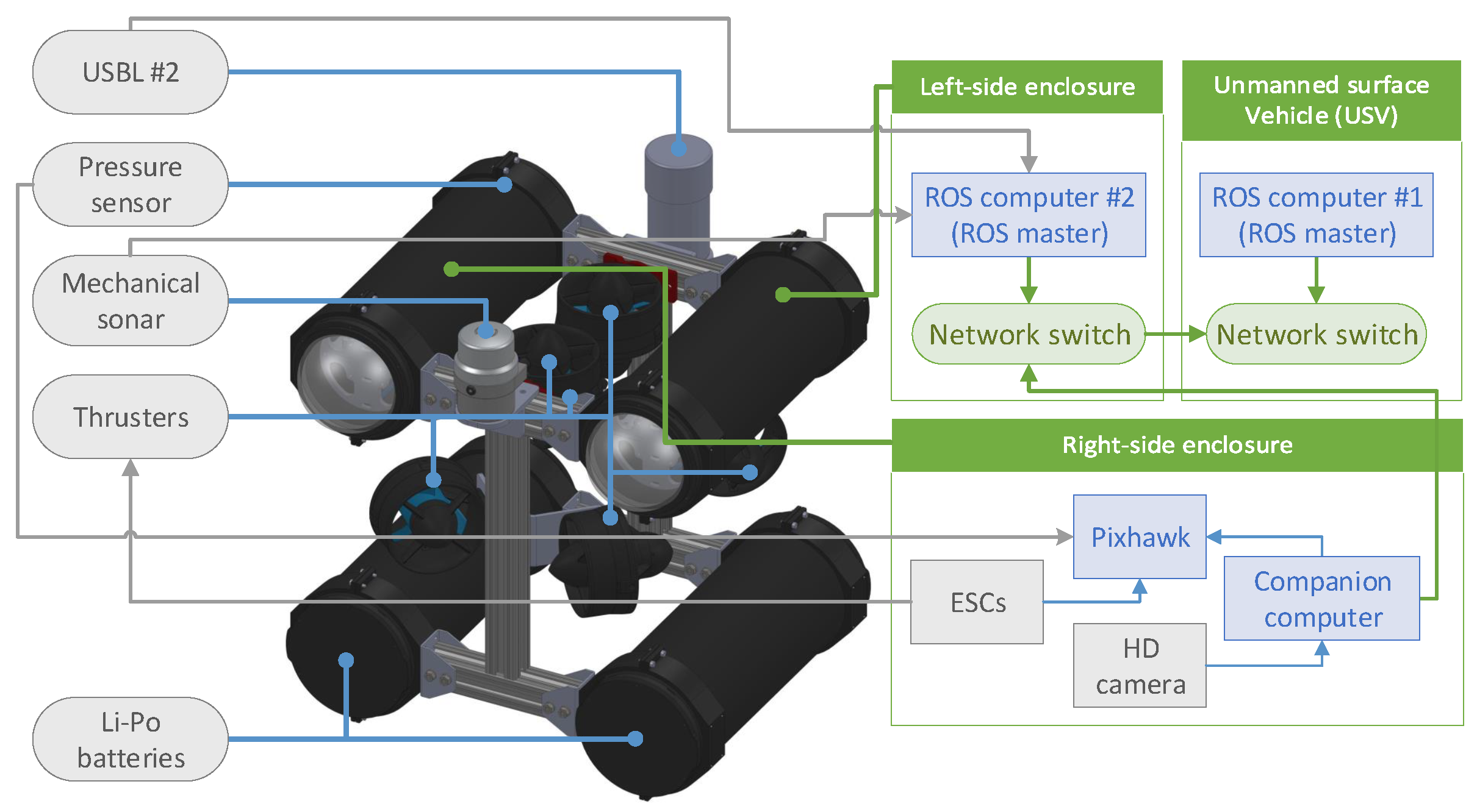
Figure 11 shows the mechatronic systems used in the AUV platform. The AUV is connected to the USV via a neutrally buoyant tether to have a direct connection between the vehicles. Similarly to the USV platform, the AUV contains high-level control with the ROS computer and an intermediate-level control as a bridge between the main ROS computer and the companion computer, which communicates using the MAVLink protocol. The low-level control includes actuators and sensors, formed by six thrusters and their respective electronic speed controllers (ESCs), a pressure sensor for depth measurements, a mechanical imaging sonar as the perception sensor, and the USBL SeaTrac acoustic system for positioning and communication. Finally, the AUV includes a companion computer with the flight controller and the ROS computer (Linux computer) connected to a network switch. The ROS computer performs the complex computations for autonomous operation and target detection.

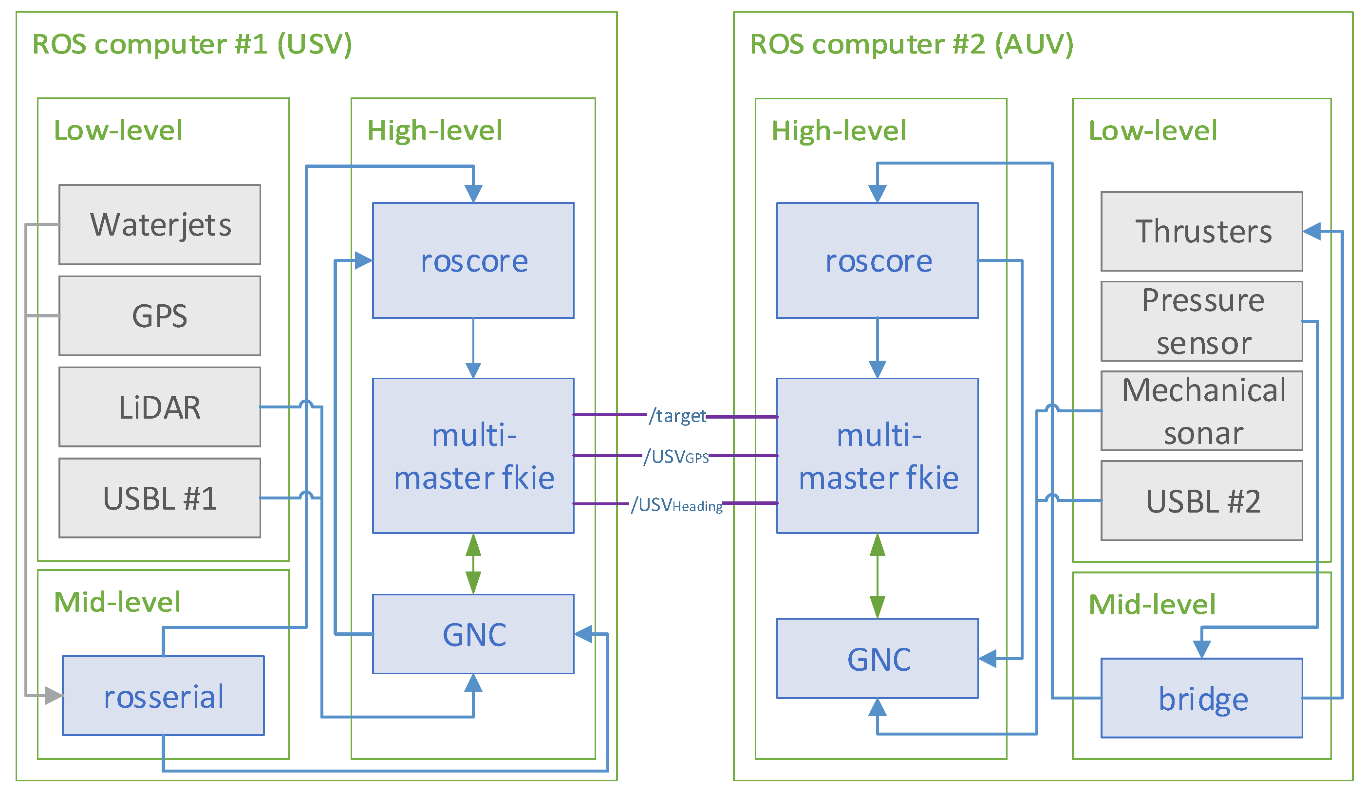
The approach used in this study for the multi-robot architecture is multimaster-fkie, which provides simplicity and ROS compatibility [21]. This package is a fully compatible multi-master implementation for topic and services transactions. Nevertheless, this implementation can cause some drawbacks due to the continuous master state scanning and the delay between changes in advertising, as well as information exchange. As this study requires a total of three ROS topics, this package is useful as an easy plug-and-play solution.

Figure 12 illustrates the communication between the USV and AUV platforms, including the nodes for the multimaster-fkie architecture. The exchanged topics are $/target$, which is the position of the detected target, $/usv\_gps$ obtained from the USV GPS-compass and used to get the absolute Cartesian coordinates of the AUV position, and $/usv\_heading$ which rotates the USBL coordinate system according to the heading of the USV. The diagram also includes the links between the high-level, mid-level, and low-level control in both platforms.

4.2. Modular System for Multi-Sensor Technology

The target detection algorithm uses a modular approach to include target detection from each perception sensor, path-following, and guidance control from both USV and AUV platforms. Each of these modules runs a separate ROS node in the autonomous offshore system. This approach has been previously studied and successfully implemented in [10,32]. However, the algorithms of the mentioned studies did not include co-operative capabilities between multiple autonomous vehicles.

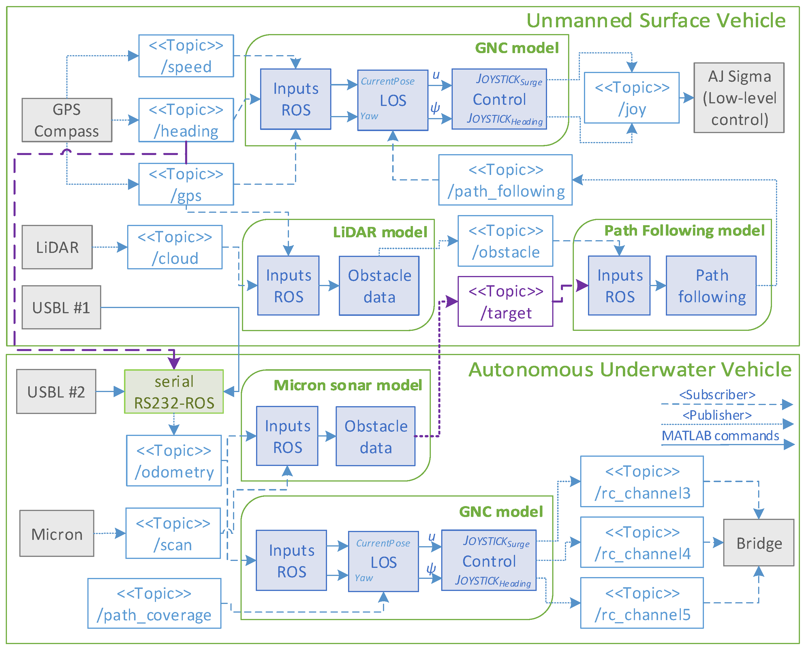
Figure 13 illustrates the modular architecture with all topics involved, defining the subscribers and publishers of each topic. The only difference between the two vehicles is the path-following model at the USV for obstacle avoidance, which is in charge of modifying the USV trajectory using the safety boundary box approach.

The GPS-Compass obtains the absolute position of the USV in global coordinates, while the USBL collects the position of the AUV in the BODY reference frame of the USBL. The ROS topic $/odometry$ in the AUV is based on the low-level serial messages accepted and generated by the SeaTrac USBL beacons [16]. These serial messages are ASCII-Hex characters of the message string, which are decoded into an array of bytes representing their values. The ROS topic is generated using the Serial package [33], which translates the RS232 messages to a ROS topic array. After that, PING messages are sent from the main USBL #1 beacon located at the USV, and the response from the AUV (USBL #2) produces the necessary serial messages containing the AUV position in the BODY USBL coordinate system. Finally, the change from this reference frame to the NED coordinate system is defined by the combination of a translation and a rotation matrix. These matrices use the initial heading of the USBL and the $/heading$ and $/gps$ variables from the GPS-Compass.

The predefined path for the AUV is defined as the ROS topic $/path\_coverage$, which includes the waypoints for the GNC algorithm in the control module. The GNC guidance algorithm generates the required AUV heading command, sending this parameter to the AUV controller. The controller generates the required inputs $/rc\_channel3$, $/rc\_channel4$, $/rc\_channel5$, and sends them to the companion computer for surge, heave, and yaw motions, respectively, based on the BlueRov-ROS-playground ROS package [34].

Regarding the USV, the exchanged ROS topic $/target$ contains the target’s origin position. Thus, once this topic is received in the path-following model, it defines the necessary waypoints to perform the autonomous mission. These waypoints are sent to the GNC model, where the LOS-algorithm calculates the required course angle for the controller. Finally, the controller generates the required joystick commands for surge $/Jo{y}_u$ and yaw $/Jo{y}_r$ to reach the LOS values. These joystick commands are sent to the low-level control (display computers) to perform the autonomous USV operation, using the same outputs as a manual three-axis joystick.

4.3. Experimental Results

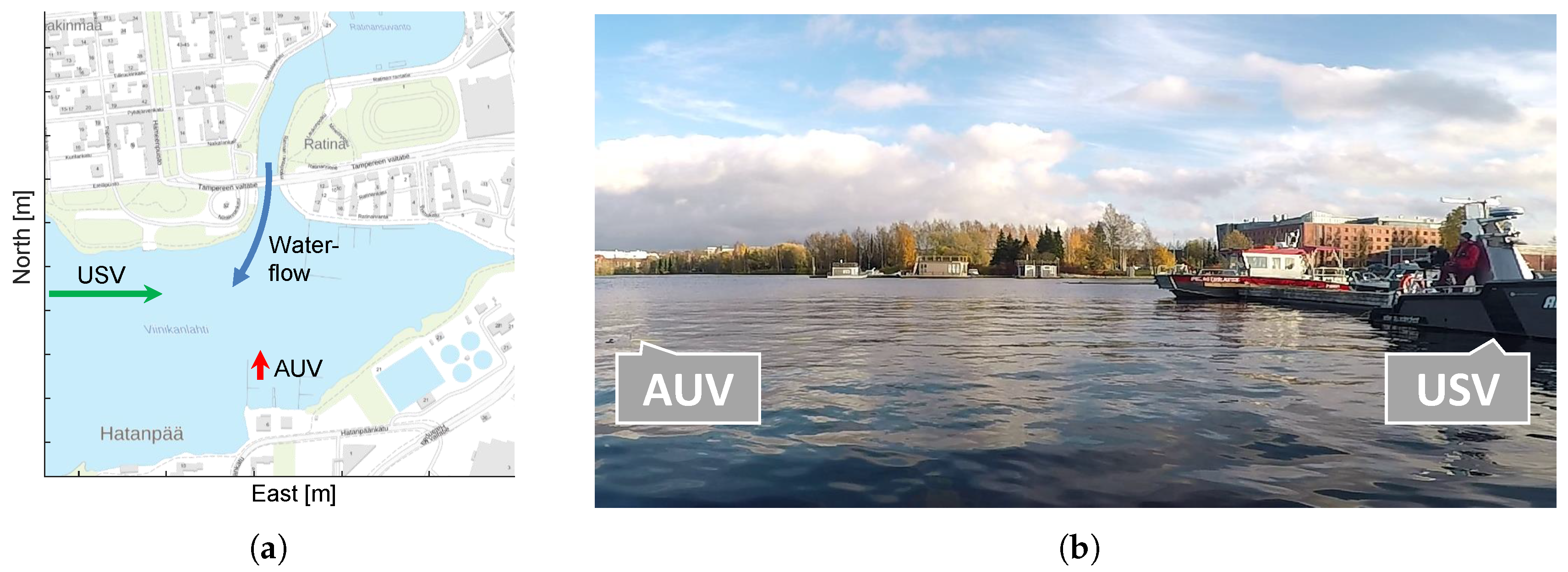
The control scenario for this study includes target detection, path-planning, and guidance control in both offshore vehicles. However, even though the modular ROS architecture provides a computationally cheap and easy implementation in both offshore platforms, the operation of both platforms in an offshore scenario depends highly on environmental elements such as wind or wave drift forces. As the guidance control bases its operation on simple PID controllers without the compensation of these environmental elements, it makes it highly challenging to gather useful field test data from the offshore system. Thus, the experimental results of this study are shown in a modular way, testing each of the subsystems separately to validate the target detection algorithm using multi-sensor technology. Figure 14a illustrates the location for the AUV and USV field tests at the Pyhäjärvi lake in Tampere, Finland. The water-flow direction from a hydro-power plant is also defined to show the environmental drift forces. Figure 14b shows the implementation for the AUV path-following, where the USV stays stationary at the harbor. Regarding the USV field test, it is demonstrated in a clear obstacle area at the lake.

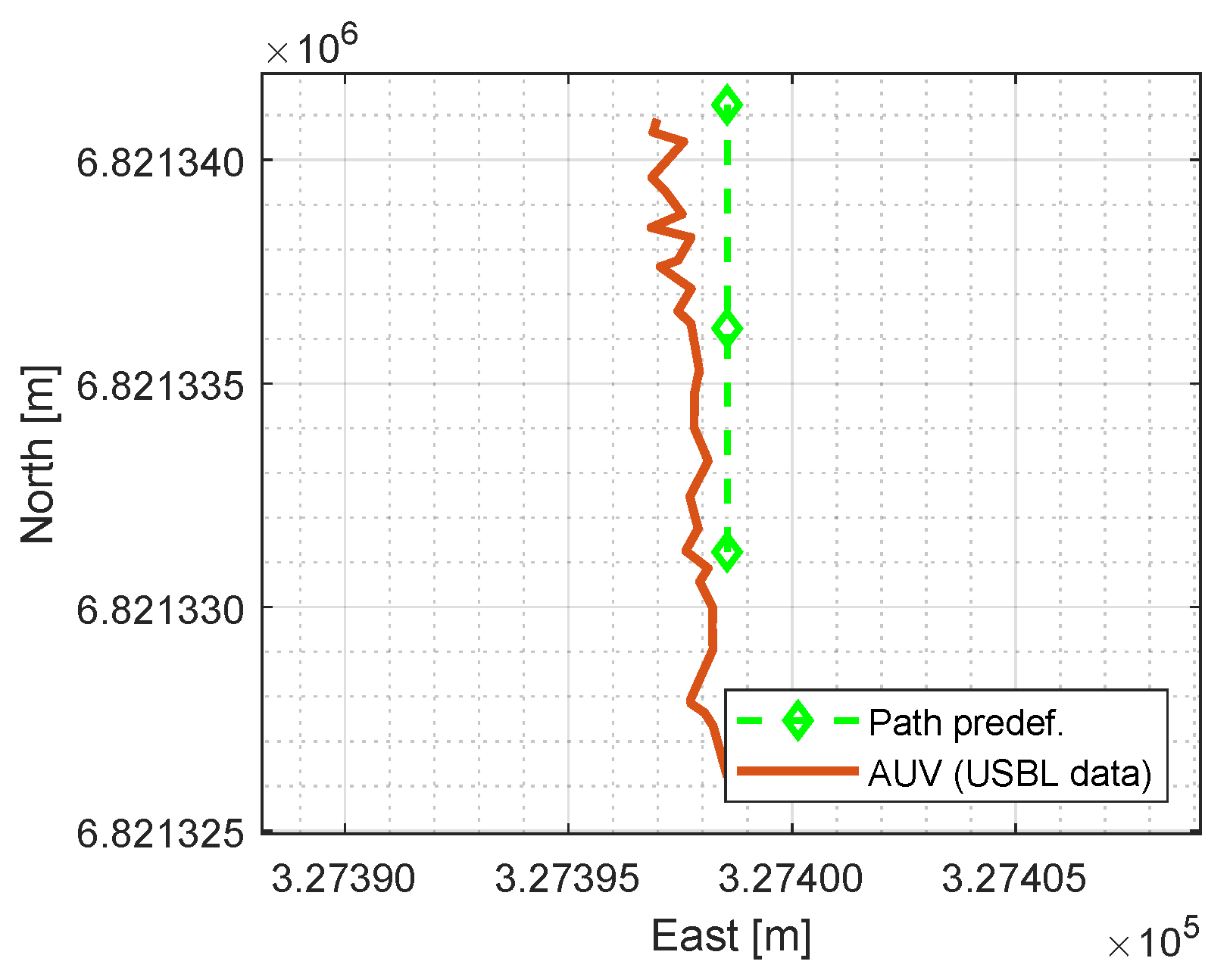
The first step in the target detection algorithm is the AUV path-following. This module is tested at the harbor with a set of three waypoints defined in the NED coordinate system. The surge motion has a constant PWM value to the thrusters, and the yaw and heave motions are implemented using separate PID controllers. The LOS-based guidance system calculates the necessary course angle to reach every waypoint of the predefined path. Figure 15 shows the AUV trajectory using the USBL data for navigation, where the AUV initial position and orientation are defined as random. The AUV moves slightly to the left side of the path-following due to the environmental drift forces. As it is shown in Figure 14a, the field tests have been done in an estuary area of a narrow and shallow lake, where the flow from a hydro-power plant affects considerably. These flow conditions vary depending on the river discharge rate. During the time of testing, the river discharge was 38 m³/s to the south direction, and the wind speed was equal to 6 m/s with southwest wind direction.

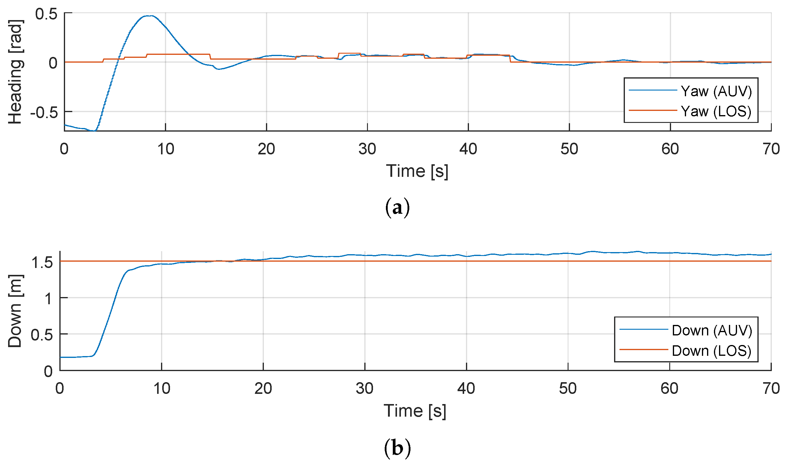
Figure 16a shows the comparison between the input control values for the yaw angle and the field test data, and Figure 16b displays the same comparison for heave motion. In this case, the multi-vehicle system contributes to the GPS-Compass data at the USV, providing the ROS topics $/gps$ and $/heading$ to the USBL acoustic system for positioning.

During the implementation of the GNC model, the target detection algorithm processes the mechanical imaging sonar data to detect and locate any possible obstacle around the AUV. Figure 7 illustrates the adequate performance of this module, where a static obstacle (buoy) is detected and located in absolute NED coordinates.

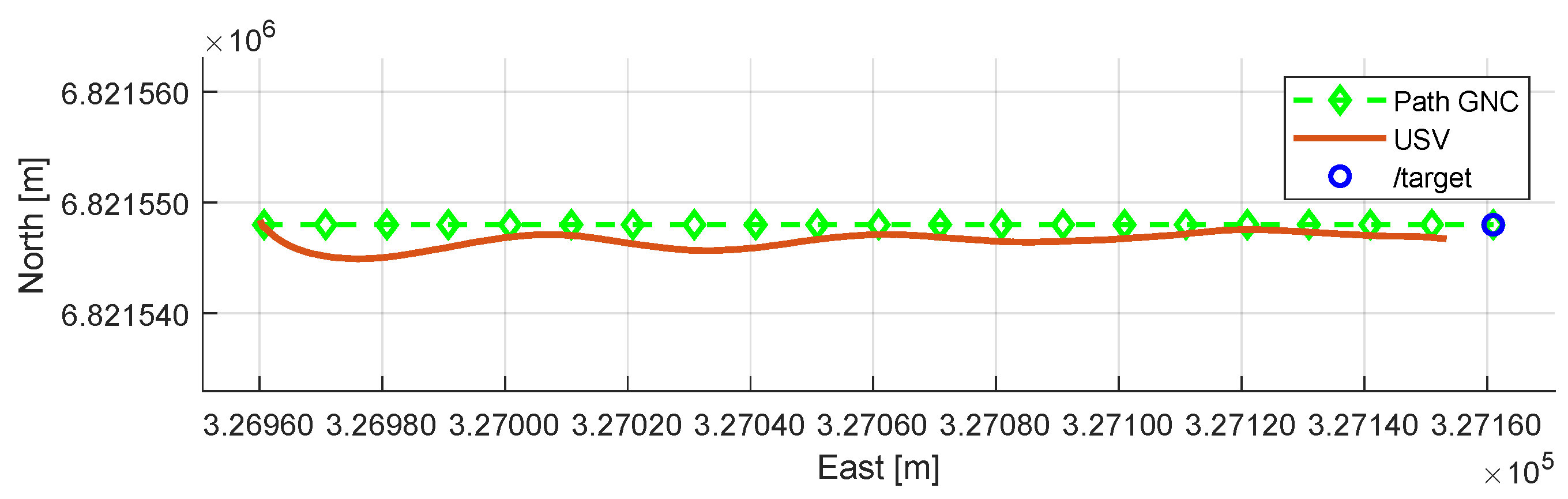
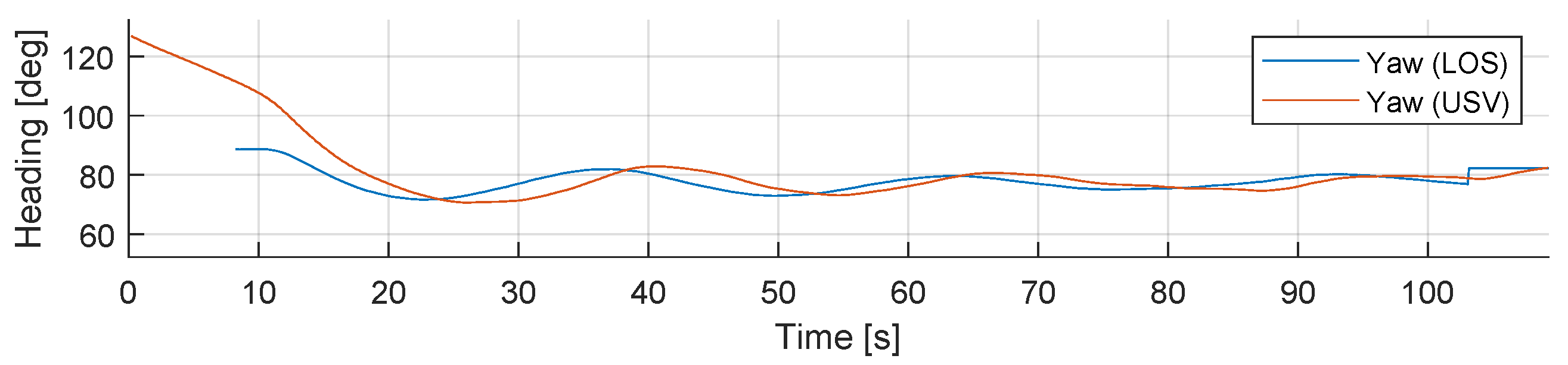
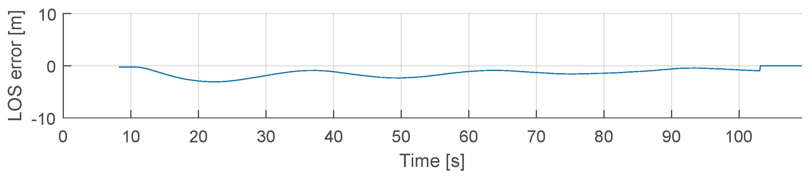
Once the AUV detects and locates the target, it sends the target’s position to the USV platform via multimaster-fkie architecture. The last control scenario in the experimental results demonstrates the co-operative autonomous offshore system with the path-following with obstacle avoidance capabilities of the USV. The USV main computer receives the $/target$ ROS topic from the AUV main computer. Then, the GNC model provides the necessary surge and yaw motions to reach the target’s position based on the LiDAR and path-following models. Figure 17 shows the USV trajectory once the path has been defined according to the ROS topic $/target$. Additionally, Figure 18 shows the comparison between the LOS guidance system and the field test data for yaw motion, and Figure 19 shows the corresponding LOS cross-track error $e\left(t\right)$, which demonstrates the correct performance of the guidance control, even though environmental variables are not considered in this study. During the USV field tests, the river discharge was 30 m³/s to the south direction, and the wind speed was equal to 3.7 m/s with south-southwest wind direction.

The experimental results of this study indicate the correct performance of the target detection algorithm using multi-sensor technology. These results are implemented in a modular way, and they show the appropriate implementation of each model, including target detection, path-following, and guidance control. The path-following algorithms in the AUV and USV platforms include some error due to the environmental variables, such as wind and wave drift forces. These variables need to be considered to increase the accuracy of the system, and they can be removed by improving the GNC controllers. Furthermore, the AUV navigation includes only the USBL beacons for positioning, which is not able to locate precisely the vehicle underwater. By improving the navigation system, the path-following algorithm will enhance its performance.

5. Conclusions and Future Work

This article was concerned with the target detection using multi-sensor technology in a co-operative autonomous offshore system. The offshore system had a USV and an AUV, and the fundamental purpose of the algorithm was to detect an underwater target in a preplanned coverage area. The mathematical model of the USV, including also the waterjet propulsion system model, was presented to verify the designed GNC architecture. This model included parameter estimation methods to obtain the dynamic coefficients using field test data for both surge and yaw motions. This study developed a basic target detection algorithm for any offshore perception sensors, showing the results for a mechanical imaging sonar at the AUV and a LiDAR at the USV. The guidance system included the LOS model for path-following on both platforms. After designing the GNC architecture, both vehicles incorporated a system implementation of the modular approach with high, intermediate, and low-level controls. The experimental results showed a field test control scenario that presents the capabilities and adequate performance of the target detection algorithm.

Future work will include an accurate mathematical model of the AUV for simulation, which requires the complete navigation data (position, velocity, and acceleration feedback) from the vehicle. Additionally, the coverage path planning can replace the straight-line trajectory of this study, having more coverage area and increasing the capabilities of the system. The AUV scenario will include the capabilities of making decisions in the presence of several obstacles, and further navigational sensors will be installed for more precise localization of the AUV (e.g., DVL). Finally, future work will also include additional platforms into the system, as it could be other USV or AUV, or even a UAV, which would increase the capabilities of the system working in the air.

References

- Vasilijević, A.; Nađ, Đ.; Mandić, F.; Mišković, N.; Vukić, Z. Coordinated navigation of surface and underwater marine robotic vehicles for ocean sampling and environmental monitoring. IEEE/ASME Trans. Mechatron. 2017, 22, 1174–1184. [Google Scholar] [CrossRef]
- Ross, J.; Lindsay, J.; Gregson, E.; Moore, A.; Patel, J.; Seto, M. Collaboration of multi-domain marine robots towards above and below-water characterization of floating targets. In Proceedings of the 2019 IEEE International Symposium on Robotic and Sensors Environments (ROSE), Ottawa, ON, Canada, 17–18 June 2019; pp. 1–7. [Google Scholar]
- Gu, N.; Peng, Z.; Wang, D.; Shi, Y.; Wang, T. Antidisturbance Coordinated Path Following Control of Robotic Autonomous Surface Vehicles: Theory and Experiment. IEEE/ASME Trans. Mechatron. 2019, 24, 2386–2396. [Google Scholar]
- Pham, H.A.; Soriano, T.; Ngo, V.H.; Gies, V. Distributed Adaptive Neural Network Control Applied to a Formation Tracking of a Group of Low-Cost Underwater Drones in Hazardous Environments. Appl. Sci. 2020, 10, 1732. [Google Scholar] [CrossRef] [Green Version]
- Fossen, T.I. Handbook of Marine Craft Hydrodynamics and Motion Control; John Wiley & Sons: New York, NY, USA, 2011. [Google Scholar]
- The MathWorks, Inc. Simulink Design Optimization User’s Guide; Release 2020a; The MathWorks, Inc.: Natick, MA, USA, 2009. [Google Scholar]
- Ljung, L. System identification. Wiley Encycl. Electr. Electron. Eng. 1999, 1–19. [Google Scholar] [CrossRef]
- The MathWorks, Inc. System Identification Toolbox User’s Guide; Release 2020a; The MathWorks, Inc.: Natick, MA, USA, 1988. [Google Scholar]
- Klinger, W.B.; Bertaska, I.R.; von Ellenrieder, K.D.; Dhanak, M.R. Control of an unmanned surface vehicle with uncertain displacement and drag. IEEE J. Ocean. Eng. 2016, 42, 458–476. [Google Scholar] [CrossRef] [Green Version]
- Villa, J.; Aaltonen, J.M.; Koskinen, K.T. Path-Following with LiDAR-based Obstacle Avoidance of an Unmanned Surface Vehicle in Harbor Conditions. IEEE/ASME Trans. Mechatron. 2020, 1812–1820. [Google Scholar] [CrossRef]
- Villar, S.A.; Solari, F.J.; Menna, B.V.; Acosta, G.G. Obstacle detection system design for an autonomous surface vehicle using a mechanical scanning sonar. In Proceedings of the 2017 XVII Workshop on Information Processing and Control (RPIC), Mar del Plata, Argentina, 20–22 September 2017; pp. 1–6. [Google Scholar]
- Ganesan, V.; Chitre, M.; Brekke, E. Robust underwater obstacle detection and collision avoidance. Auton. Robot. 2016, 40, 1165–1185. [Google Scholar] [CrossRef]
- Leonard, J.J.; Bennett, A.A.; Smith, C.M.; Jacob, H.; Feder, S. Autonomous Underwater Vehicle Navigation; MIT Marine Robotics Laboratory Technical Memorandum: Boston, MA, USA, 1998. [Google Scholar]
- Ribas, D.; Palomeras, N.; Ridao, P.; Carreras, M.; Mallios, A. Girona 500 auv: From survey to intervention. IEEE/ASME Trans. Mechatron. 2011, 17, 46–53. [Google Scholar] [CrossRef]
- Miller, P.A.; Farrell, J.A.; Zhao, Y.; Djapic, V. Autonomous underwater vehicle navigation. IEEE J. Ocean. Eng. 2010, 35, 663–678. [Google Scholar] [CrossRef]
- Neasham, J.A.; Goodfellow, G.; Sharphouse, R. Development of the “Seatrac” miniature acoustic modem and USBL positioning units for subsea robotics and diver applications. In Proceedings of the OCEANS 2015-Genova, Genoa, Italy, 18–21 May 2015; pp. 1–8. [Google Scholar]
- Font, E.G.; Bonin-Font, F.; Negre, P.L.; Massot, M.; Oliver, G. USBL integration and assessment in a multisensor navigation approach for AUVs. IFAC-PapersOnLine 2017, 50, 7905–7910. [Google Scholar] [CrossRef]
- Breivik, M.; Fossen, T.I. Path following for marine surface vessels. In Proceedings of the Oceans’ 04 MTS/IEEE Techno-Ocean’04 (IEEE Cat. No. 04CH37600), Kobe, Japan, 9–12 November 2004; Volume 4, pp. 2282–2289. [Google Scholar]
- Quigley, M.; Conley, K.; Gerkey, B.; Faust, J.; Foote, T.; Leibs, J.; Wheeler, R.; Ng, A.Y. ROS: An open-source Robot Operating System. In Proceedings of the ICRA Workshop on Open Source Software, Kobe, Japan, 12–17 May 2009; Volume 3, p. 5. [Google Scholar]
- Børhaug, E.; Pavlov, A.; Panteley, E.; Pettersen, K.Y. Straight line path following for formations of underactuated marine surface vessels. IEEE Trans. Control Syst. Technol. 2010, 19, 493–506. [Google Scholar] [CrossRef]
- Tiderko, A.; Hoeller, F.; Röhling, T. The ROS multimaster extension for simplified deployment of multi-robot systems. In Robot Operating System (ROS); Springer: Berlin/Heidelberg, Germany, 2016; pp. 629–650. [Google Scholar]
- Ollikainen, M.; Ollikainen, M. The Finnish Coordinate Reference Systems; Finnish Geodetic Institute and the National Land Survey of Finland: Masala, Finland, 2004; Available online: https://www.maanmittauslaitos.fi/sites/maanmittauslaitos.fi/files/old/Finnish_Coordinate_Systems.pdf (accessed on 11 December 2020).
- Sagatun, S.I.; Fossen, T.I. Lagrangian formulation of underwater vehicles’ dynamics. In Proceedings of the Conference Proceedings 1991 IEEE International Conference on Systems, Man, and Cybernetics, Charlottesville, VA, USA, 13–16 October 1991; pp. 1029–1034. [Google Scholar]
- Fossen, T.I. Guidance and Control of Ocean Vehicles; John Wiley & Sons: New York, NY, USA, 1994. [Google Scholar]
- g Alamarin Jet Oy. AJ 245. Available online: https://alamarinjet.com/products/jet/aj-245/ (accessed on 11 December 2020).
- Tritech International Ltd. Micron Sonar—Product Manual; 0650-SOM-00003, Issue: 02; Westhill: Aberdeenshire, UK, 2020. [Google Scholar]
- Fossen, T.; Ross, A. Nonlinear modelling, identification and control of UUVs. IEE Control Eng. Ser. 2006, 69, 13. [Google Scholar]
- Sick AG. MRS1000: Operating Instructions; 8020494/12FY/2019-04-02; Sick AG: Waldkirch, Germany, April 2019. [Google Scholar]
- Papoulias, F.A. Bifurcation analysis of line of sight vehicle guidance using sliding modes. Int. J. Bifurc. Chaos 1991, 1, 849–865. [Google Scholar] [CrossRef]
- Healey, A.J.; Lienard, D. Multivariable sliding mode control for autonomous diving and steering of unmanned underwater vehicles. IEEE J. Ocean. Eng. 1993, 18, 327–339. [Google Scholar] [CrossRef] [Green Version]
- Ziegler, J.G.; Nichols, N.B. Optimum settings for automatic controllers. Trans. ASME 1942, 64, 759–768. [Google Scholar] [CrossRef]
- Villa, J.; Aaltonen, J.; Koskinen, K.T. Model-based path planning and obstacle avoidance architecture for a twin jet Unmanned Surface Vessel. In Proceedings of the 2019 Third IEEE International Conference on Robotic Computing (IRC), Naples, Italy, 25–27 February 2019; pp. 427–428. [Google Scholar]
- Woodall, W.; Harrison, J. Serial, Cross-Platform, Serial Port Library Written in C++. Available online: http://wjwwood.io/serial/ (accessed on 11 December 2020).
- Pereira, P.J. BlueRov-ROS-Playground. Github Repository. Available online: https://github.com/patrickelectric/bluerov_ros_playground (accessed on 11 December 2020).
Figure 1.
Simplified model of the unmanned surface vehicle (USV) using the North-East-Down (NED) coordinate system. USV motion is described by surge u (linear longitudinal motion), sway v (linear transverse), and yaw motion r (turning rotation about its z-axis).
Figure 2.
Thrust force F generated by the waterjet propulsion system depending on the shaft rotational speed N.
Figure 3.
Comparison between the USV field test data and the system identification (SI) transfer functions: (a) Engine rpm . (b) Nozzle position .
Figure 4.
Schematic of the mathematical model of the USV including both waterjet propulsion system and USV dynamic models.
Figure 5.
Comparison plot between SI tool, parameter estimation (PE) app, and field test data: (a) Surge motion. (b) Heading motion.
Figure 6.
Six-thruster configuration in the AUV: (a) Simplified model of the considered vehicle using the NED coordinate system. (b) Thrust forces with their direction for each thruster.
Figure 7.
Post-processing of the mechanical imaging sonar data in the target detection algorithm: (a) Scan data acquired from sonar. (b) Post-processing based on Algorithm 1. (c) Relative position in NED with origin as [0,0] and calculation of target’s origin. (d) Absolute position in NED of the targets.
Figure 8.
Post-processing of the LiDAR in the target detection algorithm: (a) LiDAR scan data in 3D. (b) LiDAR scan data in 2D. (c) Detection area of the USV in BODY including scan data. (d) Absolute position in NED of the targets.
Figure 9.
Stateflow diagram for priority control level in the multi-vehicle guidance system. The target detection algorithm at the AUV enables the autonomous operation of the USV.
Figure 10.
System overview of the USV platform with high-level (blue boxes),intermediate-level (white boxes), and low-level control (purple boxes), including the connection to the AUV platform (adapted from [10]).
Figure 11.
System overview of the AUV: High-level (Robot Operating System (ROS) computers), intermediate-level (companion computer and Pixhawk flight controller), and low-level control (thrusters, ultra-short baseline (USBL), pressure sensor, and mechanical imaging sonar).
Figure 12.
Communication of the autonomous offshore system based on the multimaster-fkie architecture. Each vehicle shows the internal connection between the sensors and actuators with the rest of the system.
Figure 13.
Schematic of the modular multi-vehicle guidance system with target detection. All different modules from USV and autonomous underwater vehicle (AUV) were included. ROS topics , and (purple connectors) are the exchange topics in the control scenario.
Figure 14.
Control scenario: (a) Location of the AUV (red arrow) and USV (green arrow) field tests at the Pyhäjärvi lake in Tampere, Finland, being affected by the water-flow (blue arrow) from a hydro-power plant. (b) AUV and USV platforms at the harbor during the AUV field tests.
Figure 15.
AUV Control scenario: AUV trajectory for the path-following algorithm.
Figure 16.
AUV Control scenario: (a) Comparison of heading angle from the LOS guidance system with field-test data. (b) Comparison of the constant depth of 1.5 m with field-test data.
Figure 17.
USV Control scenario: USV trajectory for the path-following algorithm, where the last waypoint is equal to the ROS topic .
Figure 18.
USV Control scenario: Comparison of heading angle from the LOS guidance system with field-test data. After reaching the position, the yaw angle is equal to the constant velocity-path relative angle for DP mode.
Figure 19.
USV Control scenario: LOS cross-track error for the lookahead-based steering law defined in (22). This error is produced by the environmental variables, as the drift angle is not included in the LOS-based guidance control.