1. Introduction
The European Space Agency Climate Change Initiative on Land Surface Temperature (LST_CCI) aims to provide Land Surface Temperature (LST) Essential Climate Variable (ECV) products and validate these data to provide an accurate view of temperatures across land surfaces globally for the past 20 to 25 years. In order to identify the best algorithms for a future climate quality operational system, an open algorithm intercomparison is needed. The purpose of this intercomparison exercise is to assess the performance of a number of different LST retrieval algorithms across multiple satellite sensors, namely, the Advanced Along-Track Scanning Radiometer (AATSR), Terra Moderate-Resolution Imaging Spectroradiometer (MODIS), Spinning Enhanced Visible and Infrared Imager (SEVIRI), Special Sensor Microwave/Imagers (SSM/I) and Special Sensor Microwave Imagers Sounder (SSMIS). This comparison is performed for a number of different products including the single-sensor LST record datasets as well as a climate data record (CDR), which combines data from AATSR, SLSTR and MODIS into a harmonized record, and finally a merged low Earth orbit/geostationary product using data from AATSR, MODIS and SEVIRI. To this end, only retrieval algorithms that can function with the minimum number of available spectral channels are considered. As the maximum number of thermal channels present across all the thermal infrared (TIR) sensors in this study is two, algorithms investigated include split-window algorithm variants and an inversion technique which is adapted to work with two channels. For the microwave (MW) sensors, both linear regression and neural network algorithms are investigated.
In the TIR region of the electromagnetic spectrum, absorption and emission effects, mainly due to the presence of water vapor, are responsible for attenuation of the surface signal observed by a satellite radiometer [
1,
2]. As such, instruments on satellites designed for retrieval of the Earth’s surface temperature use spectral windows where absorption and emission effects are minimized and the surface emission signal is higher. Both the 3.5 to 4.2 μm window and the 10.5 to 12.5 μm window are options but the former is subject to a noticeable contribution from the solar signal. Therefore the latter is most often used for LST retrieval purposes and is commonly referred to in the literature as the split-window region. Even in this region of high transmission, correcting for atmospheric attenuation is still necessary for accurate LST retrievals. Accurate LST retrieval requires algorithms which correct for both atmospheric and emissivity effects. In practice, this cannot be achieved with a full physical representation of the radiative transfer of the system from surface emission to instrument observation [
3,
4]. The radiative transfer equation and the direct inversion procedure to extract the surface temperature (
Ts) highlight the principle challenges in TIR LST retrieval, primarily being that the ground-level radiance still includes an atmospheric contribution due to the reflection term and that the coupling between surface temperature and surface emissivity is an ill-posed problem, whereby
n sensor bands will generate
n equations but
n + 1 unknowns. Therefore the retrieval of LST requires a priori knowledge of Land Surface Emissivity (LSE).
LST can, in principle, be derived from microwave (MW) measurements which are minimally impacted by cloud in the absence of precipitation [
5,
6]. With an average of ~67% cloud cover at any moment on Earth [
7], MW LST estimation can be a key complement to TIR LST estimates which have a clear sky bias due to clouds obscuring observation at these wavelengths. However, retrieving LST from MW observations is still challenging. First, the MW signal from the surface is highly sensitive to the product of the emissivity and the surface temperature as the atmospheric contribution is negligible compared with the TIR. This relationship means that the MW signal has a stronger dependence on the emissivity. Furthermore, the MW emissivity varies more with surface properties such as soil moisture, vegetation cover, or the presence of snow, surface roughness, and shows spatial and temporal variability that needs to be accounted for in the retrieval. In addition, the spatial resolution of the MW observations degrades with decreasing frequency, whereas the atmospheric contribution to the signal tends to increase with frequency. The spatial resolution of the current MW imagers is typically 10 to 20 km at the frequencies (~19 to 90 GHz) used for LST retrieval, a factor of 10 to 100 times coarser than current TIR observations [
8,
9].
Due to differences in instruments and the difficulties in deriving LST from satellite remote sensing outlined above, a number of different methodologies have been developed each usually tailored to a particular instrument. With a large number of algorithms in both the TIR and MW it is impossible to fully harmonize different datasets. There have been a number of studies looking to assess the different algorithm performances of LST algorithms [
10,
11,
12,
13,
14,
15,
16,
17,
18]. However, these studies use in situ validation sites. While this is an excellent metric for point-based bias assessment, it runs into significant issues. Firstly, there are very few sites across the globe and their distribution is not representative of the range of biomes present globally as most sites are in Europe and Northern America [
13,
19]. This is critically important as biome classifications provide a realistic range of atmospheres and surfaces, which capture the real-world coupling between different regions and the conditions observed there. Secondly, due to the low number of validation sites, many of them have been used in the development and training of the algorithms under study in this assessment, making it difficult to separate out the station-dependent biases in testing. Thirdly, the sensor differences in view angle and pixel footprint size mean that the intercomparisons between validation sites and different instruments are not always readily intercomparable due to site heterogeneity [
20,
21,
22].
This study presents an intercomparison of various algorithms over multiple sensors, rather than an intercomparison over a single satellite sensor, and as such demonstrates the consistency and robustness over the multiple systems. This is a critical requirement when looking to combine data from different sensors and moving towards a climate quality data record. This study uses model re-analyses and globally available surface information to create a benchmark database consisting of a large number of atmospheric and surface parameters, which vary so as to test each algorithm and sensor under a wide variety of physically realistic conditions. This methodology enables the fair intercomparison of algorithms under identical situations, with no training biases, and over a range of conditions that fully assess their global applicability.
The method, including the construction of the benchmark database and assessment methodology are described in
Section 2. Results for both the TIR and the MV sensors for all algorithms are shown in
Section 3. A discussion is provided in
Section 4, including an examination of each algorithms performance of the various sensors under study and how their performance could be improved. Conclusions are provided in
Section 5.
2. Materials and Methods
2.1. Algorithms
The following section outlines the different algorithms studied in this work—a summary of the TIR algorithms can be seen in
Table 1, and of the MW algorithms in
Table 2.
2.1.1. University of Leicester Biome-Based Algorithm (UOL)
The standard (A)ATSR and SLSTR LST algorithm [
1] uses a nadir-only split-window (SW) algorithm with classes of coefficients for each combination of biome-diurnal (day/night) condition. The physics in principle are the same as for other SW algorithms, such as [
11], which also apply coefficients to a combination of emissivity, water vapor and BT differences. In [
11], non-linearity is accounted for in the quadratic term, whereas here it is parameterized across the swath. The full form of the algorithm is presented as follows:
where
T11 and
T12 are the top of atmosphere brightness temperatures for the 11 and 12 micron channels, respectively. The six retrieval coefficients
as,i,
av,i,
bs,i,
bv,i,
cs,i and
cv,i are dependent on the biome (
i), fractional vegetation cover (f)—the retrieval coefficients
as,i,
bs,i and
cs,i relate to bare soil (
f = 0) conditions, and
av,i,
bv,i and
cv,i relate to fully vegetated (
f = 1) conditions. The fractional vegetation cover (
f) and precipitable water (
pw) are seasonally dependent whereas the biome (
i) is invariant [
23].
The retrieval parameters
d and
m are empirically determined from validation and control the behavior of the algorithm for each zenith-viewing angle (
θ) across the nadir swath. The parameter
d resolves the increase in atmospheric attenuation due to water vapor with increasing zenith viewing angle. The parameter
m is supported by previous studies [
23], which suggest that a non-linear term dependent on the BT difference,
T11–T12, would elicit improvement in the accuracy of the LST retrievals. The rationale here is that the BT difference increases with increasing atmospheric water vapor since attenuation due to water vapor is greater at 12 μm than at 11 μm.
The nature of the algorithm means that LSE is implicitly dealt with through the regression of retrieval coefficients to biome and bare soil/fully vegetated states. In other words, while LSE is not an estimated output the algorithm still uses LSE knowledge, any uncertainty in which is propagated in the LST derivation. This knowledge is passed to the algorithm through the biome and fractional vegetation states, which themselves are regressed to emissivity states in the coefficient generation.
For the generation of the retrieval coefficients for each biome–diurnal (day/night) combination vertical atmospheric profiles of temperature, ozone, and water vapor, surface and near-surface conditions and the surface emissivity are required. These are input, in addition to specifying the spectral response functions of the instrument, into a radiative transfer model in order to simulate top-of-atmosphere (TOA) BTs. Retrieval coefficients are determined by minimizing the l2-norm of the model fitting error (ΔLST).
2.1.2. Generalized Split Window (GSW)
The GSW algorithm proposed by Wan and Dozier [
24] is based on channels centered at approximately 11 and 12 µm. This method, unlike the AATSR/SLSTR split-window method, uses explicitly stated emissivity rather than incorporating this information implicitly through biome coefficients.
In the operational MODIS and SEVIRI implementations, band averaged emissivity for each of the two channels are used.
where
and
are the upper and lower bounds of the channel,
is its spectral response function, and
is the surface temperature. This parameter is assigned on a pixel basis according to land cover class. In cases of mixed pixels this term is recalculated based upon the proportion of the pixel assigned to each classification.
Having determined the emissivity of the pixel coefficients, these can be applied to derive an LST estimate.
where C, A, and B are coefficients derived from linear regression using simulated data.
is the mean emissivity of the two thermal channels and
is the difference between them. The coefficients are dependent on satellite viewing angle, water vapor and atmospheric temperature.
2.1.3. Quadratic Split Window (QSW)
The quadratic split-window (QSW) algorithm is a variant on the GSW algorithm first proposed by [
24]. The QSW algorithm [
15] includes a refinement, which is particularly adapted for use over bare soils. The rationale being that the large variations in surface emissivity in between the 11 and 12 µm channels for bare soils and the increased probability of higher atmospheric load of dust aerosols over these regions requires an additional quadratic component:
As in the case of the GSW, the
A,
B and
C coefficients are dependent on satellite viewing angle, water vapor and atmospheric temperature. Ref. [
15] performed comparisons of the LST error statistics, and these indicate that retrieval accuracy may improve with the addition of the quadratic term compared with GSW. The quadratic term may, however, lead to large LST uncertainty under higher water vapor conditions [
15], and this may limit its applicability to climate datasets.
2.1.4. Enterprise Algorithm (ELA)
The Enterprise LST Algorithm (ELA) is the operationally implemented algorithm for the Visible Infrared Imaging Radiometer Suite (VIIRS) LST product, produced by the National Oceanic and Atmospheric Administration (NOAA). It is another split-window which requires explicit emissivity information [
25]:
where
C and
A are retrieval algorithm coefficients which, for the operational enterprise algorithm, are dependent on sensor zenith angle, day-night flag, and total precipitable water. There are a total of 30 sets of coefficients for all combinations of these three dimensions: sensor zenith angle has 5 intervals; total precipitable water has 3 intervals; and the day-night flag has 2 intervals.
2.1.5. Synergistic Algorithm for Sentinel LST (SYN)
SYN is developed offline for Sentinel-3 for synergistic use with Sentinel-2. Specifically, the use of explicit LSE estimates derived from Sentinel-2 in the LST algorithm for Sentinel-3 [
26]. The mathematical structure is given by:
where
pw is the atmospheric water vapor content. The split-window coefficients
cx are obtained from simulation. Because of the explicit dependence on emissivity for this SW algorithm, the coefficients are independent of the biome and the Fractional Vegetation Cover (FVC). The derivation of the coefficients is performed through statistical regression from a benchmark database of at-sensor brightness temperatures and surface emissivity (laboratory samples) over different atmospheric conditions.
2.1.6. Optimal Estimation (OE)
Optimal Estimation (OE) is a technique that has proven to be of great use in Earth Observation, specifically in resolving multispectral measurements to give multilevel atmospheric profiles. OE exploits a priori knowledge of the surface and atmospheric parameters to generate simulated Brightness Temperatures (BTs), which are mathematically compared to the actual observed BTs. The offset between the simulated and observed BTs is used to inform updates to the retrieved parameters.
For an EO satellite which observes TOA BTs at
m different wavelengths, the measurements are collated into the single observation vector (
). The objective is to retrieve a profile (
), containing
n different atmospheric and/or surface parameters. If the actual state of the atmosphere and surface was known at the time of observation, then:
where
represents the Forward Model, which computes the radiative transfer process based on the input profile (
), and
is the combined forward model and measurement error. The Bayesian approach allows the algorithm to improve upon the initial first guess surface parameters.
The OE retrieval follows the underlying methodology of [
27]. The prior surface parameters are fed into a radiative transfer model (RTM) and used to simulate TOA BT for each of the instrument channels. The quality of the simulated TOA BT and hence the surface information used to generate it is evaluated by the cost function:
The OE approach used here was developed by Perry [
28] for TIR retrievals from satellite. In order to improve the retrieved results, multiple iterations are performed building upon the previous results to reduce the residuals between the observed and simulated BTs considering the a priori parameters. In this retrieval the cost function is a measure of the agreement between the retrieved parameters and the a priori parameters, and residual of the simulated and real BTs.
2.1.7. MW Algorithms
Based on the objective of deriving a seamless data record of MW LST for climatological applications, a number of statistical retrieval algorithms for MW LST will be calibrated and tested with a benchmark database simulating brightness temperatures at 19.35, 22.235, 37.0, and 85.5 GHz. In essence the algorithms differ in the number of channels used in the retrieval, the application of pre-calculated emissivity to constrain the inversion problem, and the type of regression.
2.1.8. Number of Channels
In principle, the vertically polarized 37.0 GHz channel is the best suited for mono-channel LST estimation by combining a reduced sensitivity to soil surface characteristics with a relatively high atmospheric transmission [
29]. Adding the remaining channels, with both vertical and horizontal polarizations, should help to constrain the inversion problem by adding further information about the surface state (19.35 GHz and 85.5 GHz) and atmospheric contribution to the signal (22.235 GHz for water vapor absorption, and the 85.5 GHz for cloud scattering).
2.1.9. Use of Emissivity
Given the large impact LSE can have on the MW signal, the use of pre-calculated MW emissivity should result in more accurate inversions. This will especially be the case at locations where the emissivity has a greater departure from typical values (e.g., arid places, humid regions, wetlands, snow-covered terrain). For the same reasons, regions with large temporal variability in surface conditions may not be properly accounted by a climatological emissivity (e.g., changing ground conditions due to snow, frozen and melting). Consequently, retrievals incorporating a climatological emissivity may still be problematic at those locations [
8].
2.1.10. Type of Regression
For a given observation frequency, the surface contribution to the brightness temperatures is directly proportional to the LST and the emissivity. Therefore, it could be argued that linear regressions may be sufficient for a first good approximation. In practice, the simultaneous use of observations at different frequencies, together with the need to also account for the atmospheric contribution to the observed signal, results in a relatively complex relationship. Accordingly, models allowing a non-linear relationship may be better suited [
30].
Here, non-linear regression models are implemented by means of a neural network (NN). The NN is based on a standard three-layer perceptron with an input layer having as many nodes as the number of frequency channels (and associated emissivity if used), followed by a hidden layer, and an output layer with one node for the retrieved LST. The NN initial weights are initialized as in [
31], and the final weights assigned by a Marquardt-Levenberg back-propagation algorithm [
32]. To prevent over-fitting to the training dataset, a cross-validation technique is used to monitor the evolution of the training error function.
2.1.11. Implemented Algorithms
In practical terms, the combination of different number of channels, use of the emissivity, and type of regression, results in a relatively large number of possible algorithms. Only the results from a number of them are presented here to demonstrate the retrieval performance. They are summarized in
Table 2. Notice that for all algorithms a strategy of having separate regressions for (1) Greenland and Antarctic, and (2) the remaining continental land is adopted. Permanent snow results in a particular set of brightness temperatures and emissivity conditions, and a separate regression over those areas benefits the retrievals conducted here [
30].
2.2. Satellite Sensors
The Along-Track Scanning Radiometer (ATSR) instruments, ATSR-1, ATSR-2 and AATSR (Advanced Along-Track Scanning Radiometer), were launched on board European Space Agency (ESA) sun synchronous, polar orbiting satellites ERS-1 (European Remote-Sensing Satellite-1) launched in July 1991, ERS-2 launched in April 1995, and Envisat (Environmental Satellite) launched in March 2002, respectively. The third of these instruments—AATSR—provided its last data on 8th April 2012. The ATSRs therefore provide approximately 20 years of data. Continuation of this sensor series occurred, albeit with a data gap, with the launch of the Sea and Land Surface Temperature Radiometer (SLSTR) sensors on board Sentinel-3 satellites. All ATSR instruments used similar orbits and equator crossing times ensuring a high level of consistency. With a swath width of 512km, AATSR is able to provide approximately 3-day global LST coverage with a repeat cycle of 35 days. The overpasses of AATSR in local solar time are 10:00 in its descending node and 22:00 in its ascending node. For ATSR-2 and ATSR-1 the overpass times are 10:30 and 22:30 in the descending and ascending nodes, respectively. The orbits of the ATSRs were very stable in local equator crossing times and no notable orbital drifts occurred [
33].
MODIS is the name of two current instruments mounted on the NASA satellites Terra and Aqua, launched in 1999 and 2002, respectively. The two satellites are on orbits that allow different temporal insight in the observations. For example, over the UK the MODIS on Terra will record an image in the morning and the early night, whereas Aqua will observe at midday and midnight [
34]. The local equatorial crossing times are 10:30 am and 1:30 pm for Terra and Aqua, respectively. MODIS was designed to improve knowledge globally in the areas of land, ocean and lower atmospheric processes. Additionally MODIS aimed to continue and enrich the data record associated with heritage missions such as the Advanced very-high-resolution radiometer (AVHRR), High resolution Infrared Radiation Sounder (HIRS) and Landsat TM [
35]. Using both Aqua and Terra MODIS sensors enables us to monitor and analyze short term climate and environmental phenomena. MODIS has 36 spectral bands ranging from the visible through the near-infrared to the TIR, each focused on a variety of different scientific objectives and with spatial resolutions varying from 250 m to 1 km.
SEVIRI is the main sensor on board Meteosat Second Generation (MSG), a series of 4 geostationary satellites operated by EUMETSAT. SEVIRI was designed to observe an Earth disk over Africa, most of Europe and part of South America with a temporal sampling of 15 min. Satellite view angles for SEVIRI range from 0° to 80°. The first MSG satellite was launched in August 2002, and operational observations are available since January 2004. SEVIRI spectral characteristics and accuracy, with 12 channels covering the visible to the infrared [
36] were unique among sensors on board geostationary platforms for several years after the launch of MSG-1. The infrared channels have a spatial resolution of 3 km at the centre of the viewing disk. Level 1.5 data are disseminated to users after being rectified to 0° longitude, which means that the satellite viewing geometry varies slightly with the acquisition time.
The MW LST product will be built using radiances observed by SSM/I since 1987 and its more recent version SSMIS since 2003. This family of instruments flies on board Defense Meteorological Satellite Program (DMSP) near-polar orbiting satellites, and provides passive MW observations twice a day at 19.35, 22.235, 37.0, and 85.5 (SSM/I) or 91.665 (SSMIS) GHz with an incident angle of 53° resulting in ground resolutions for SSM/I (SSMIS) of 69 × 43 (73 × 41), 50 × 40 (73 × 41), 37 × 28 (41 × 31), and 15 × 13 (14 × 13) km, respectively. Vertically and horizontally polarized brightness temperatures are available at all frequencies, apart from the 22.235 GHz channel, which is only vertically polarized. Instrument swath widths are close to 1400 (SSM/I) and 1700 (SSMIS) km, providing a 1–2 days revisiting time depending on acquisition latitude. The source of BTs will be the EUMETSAT Satellite Application Facility on Climate Monitoring (CM SAF) Fundamental Climate Data Record of Microwave Imager Radiances [
37], where the BTs from the different SSM/I and SSMIS instruments have been intercalibrated to reduce changes related to intersensor differences.
2.3. Benchmark Database
In constructing a method for selecting the best algorithm for different sensors, an assessment of the available data with which to test the algorithms is key. Ideally the use of well-calibrated and globally distributed in situ sensors would provide the benchmark against which the retrieved LSTs can be tested. However, in the study of LST, there are relatively few high quality in situ stations available to validate satellite-derived LST data, which are often clustered in certain regions. More problematically, due to the small number of stations, many of the algorithms to be tested have been extensively trained on these sites. This leads to two key issues: firstly, insufficient in situ stations to build a match-up database for global analysis; and secondly, some algorithms are trained to the paucity of in situ matchups available and thus are likely to perform well for these limited conditions, but performance may be poor elsewhere.
The alternative to using in situ data is to assess the algorithms from a theoretical basis using a benchmark database. This approach covers a wide range of both surface and atmosphere conditions and is thus more likely to be representative of real environments on a global scale. Simulated data necessitates the use of modelled atmospheric data and ancillary sources for emissivity, fractional vegetation and biome information. All of these inputs are used with a common forward model to result in useful and robust data at both the surface level and for the observed TOA BTs.
The ERA5 dataset is the successor to the ERA-Interim Re-analysis dataset [
38]. This dataset is a re-analysis, which provides hourly estimates of a significant number of land and atmospheric variables over the full globe. ERA5 currently has a temporal coverage similar to other re-analyses (from 1979 to present), but more years are to be added to extend this dataset back to 1950. The dataset provides full atmospheric parameters required for the accurate simulation of atmosphere and surface parameters such as elevation and LST at a resolution of 0.25°. The benchmark dataset in this intercomparison uses data from 2013 to 2015.
The Combined ASTER and MODIS Emissivity for Land (CAMEL) database provides a global monthly mean emissivity dataset spanning the years 2000–2016. It assimilates the ASTER Global Emissivity Database (GED) retrieved values and the University of Wisconsin-Madison MODIS Infrared Emissivity dataset (UWIREMIS) values. The resulting dataset contains 12 emissivity values at different wavelengths from 3.6 to 14.3 µm at a resolution of 0.5° [
39]. Due to the dataset originating from satellite observations, it is highly relevant to realistic materials observed from space and should remove materials in spectral libraries, which are of too fine a scale to be useful. The benchmark dataset and the retrievals tested in this study use wavelengths of 10.8, 11.3 and 12.1 µm.
The FVC is drawn from the Copernicus Global Land Services (CGLS) FCOVER dataset. This is available globally at 1/112° spatial resolution every 10 days from 1999 onward and acquired from a moving temporal window of approximately 30 days [
40]. The validation of the product is described in Camacho et al. [
41], who conclude that the product shows good quality with a spatially consistent global distribution of retrievals.
A Tool to Estimate Land Surface Emissivities at Microwave frequencies (TELSEM) provides a global monthly mean emissivity dataset designed to integrate with the RTTOV forward model (see next section). The data are based on SSM/I observations at 0.25° resolution, which matches the ERA5 and reduces the need for spatial interpolation. The emissivity data are produced at frequencies of 19.35, 22.235, 37.0 and 85.5 GHz in both vertical and horizontal polarizations forming a climatology of 8 years of data spanning the period 1993–2003 [
42]. All channels are used in the generation of the benchmark database and in the MW retrievals.
Radiative Transfer for TOVS (RTTOV) is a fast radiative transfer model (RTM) developed within ECMWF and subsequently by the UK Met Office, Meteo-France under the EUMETSAT funded NWP-SAF [
43]. It is an efficient forward model for radiative transfer in the visible, TIR and MW. RTTOV is used for all algorithms and for the generation of all benchmark database BTs. Using a single forward model provides consistent and meaningful comparison of retrieval algorithms. Additionally RTTOV is faster than line-by-line models providing the ability to process large numbers of profiles for a statistically significant sample size [
44]. RTTOV version 11.3 is used for all processing in this study with version 9 coefficient files. All emissivities, both MW and TIR, are fed in externally to avoid internal interpolation and provide traceability. It is important to note that all simulations used in this testing assume nadir observing conditions. View angle is a highly influential factor in TIR retrievals and would be expected to be a significant contributor to the radiative transfer process. All the algorithms under study here have the ability to work at off-nadir view angles either through radiative transfer simulation or banding of the linear regression coefficients, the off-nadir retrievals still have the potential to be optimal because the banding is meant to minimize retrieval differences as a result of different view angles. Testing these algorithms over variable view angles is out of the scope of this work but expected to be the subject of further study building on this work.
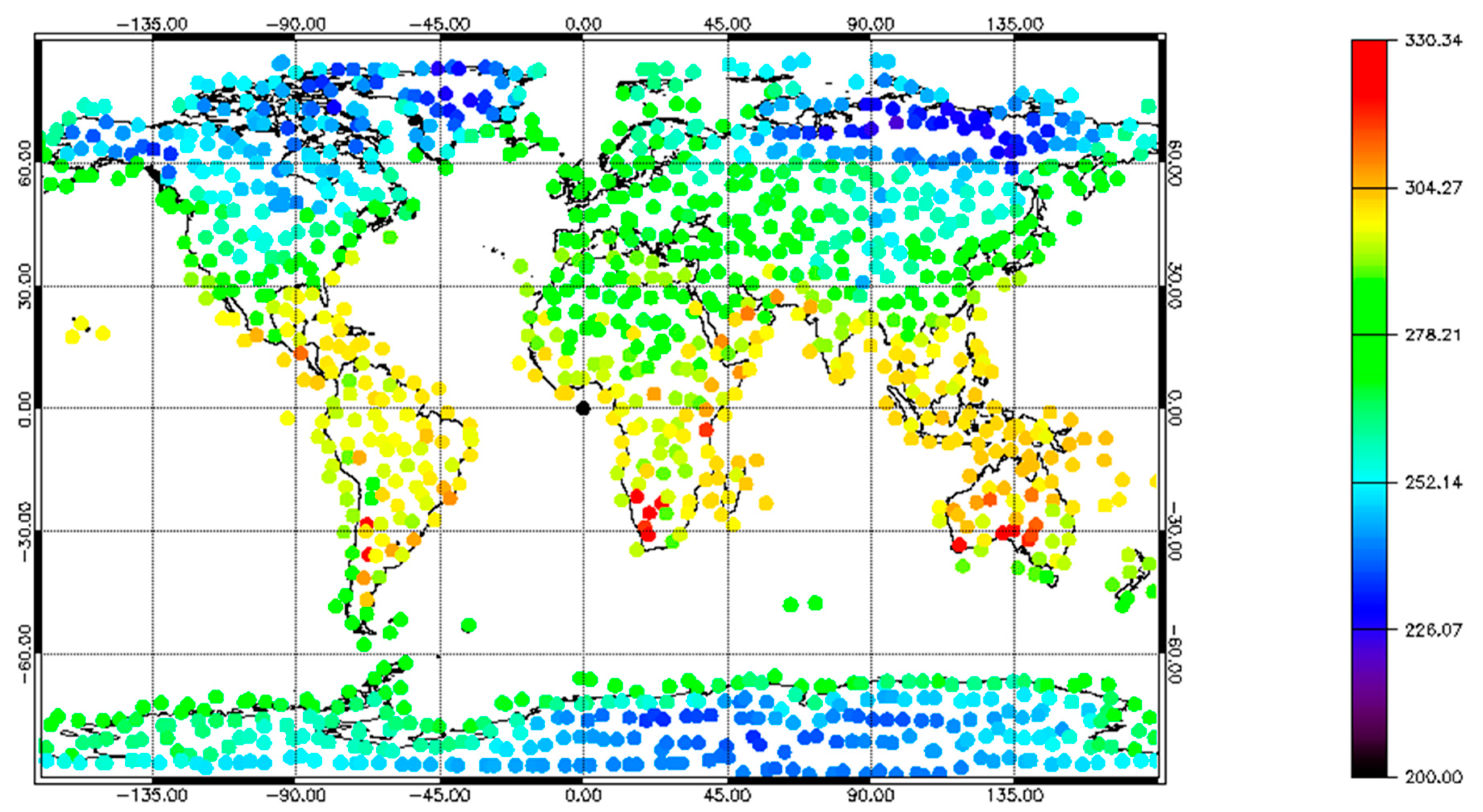
In constructing the benchmark database, the initial parameter considered is the atmosphere, primarily focusing on the water vapor as the most significant influence on the retrieval of LST. All selected profiles are drawn from cloud free data. The ERA5 data are gridded at 0.25 degree resolution and contains both full water vapor profiles as well as the total column water vapor (TCWV) values. Averaging the full profile can result in an overly smoothed product, which might not be representative of real atmospheres. To avoid this, the ERA5 data are gridded into cells of 5 × 5° and the mean TCWV values for each cell calculated. The mean total column water vapor is then compared to all the TCWV values in the 5 × 5° grid cell. The profile that corresponds to the closest matching TCWV value is selected as the representative profile for the grid cell. This methodology ensures that not only is the profile physically realistic but that it represents the most likely conditions for the majority of the grid cell. This is important when comparing to other parameters such as biome and LSE which are sourced from different datasets. Climatologies for the grid cells are made and the standard deviations of the TCWV compared. The range of variation is in line with the variation seen in the selected dataset. All other information such as LST, elevation, and other gas profiles are also selected using the index of this profile. An example of the Skin Temperature (Tskin) from the ERA5 dataset is shown in
Figure 1.
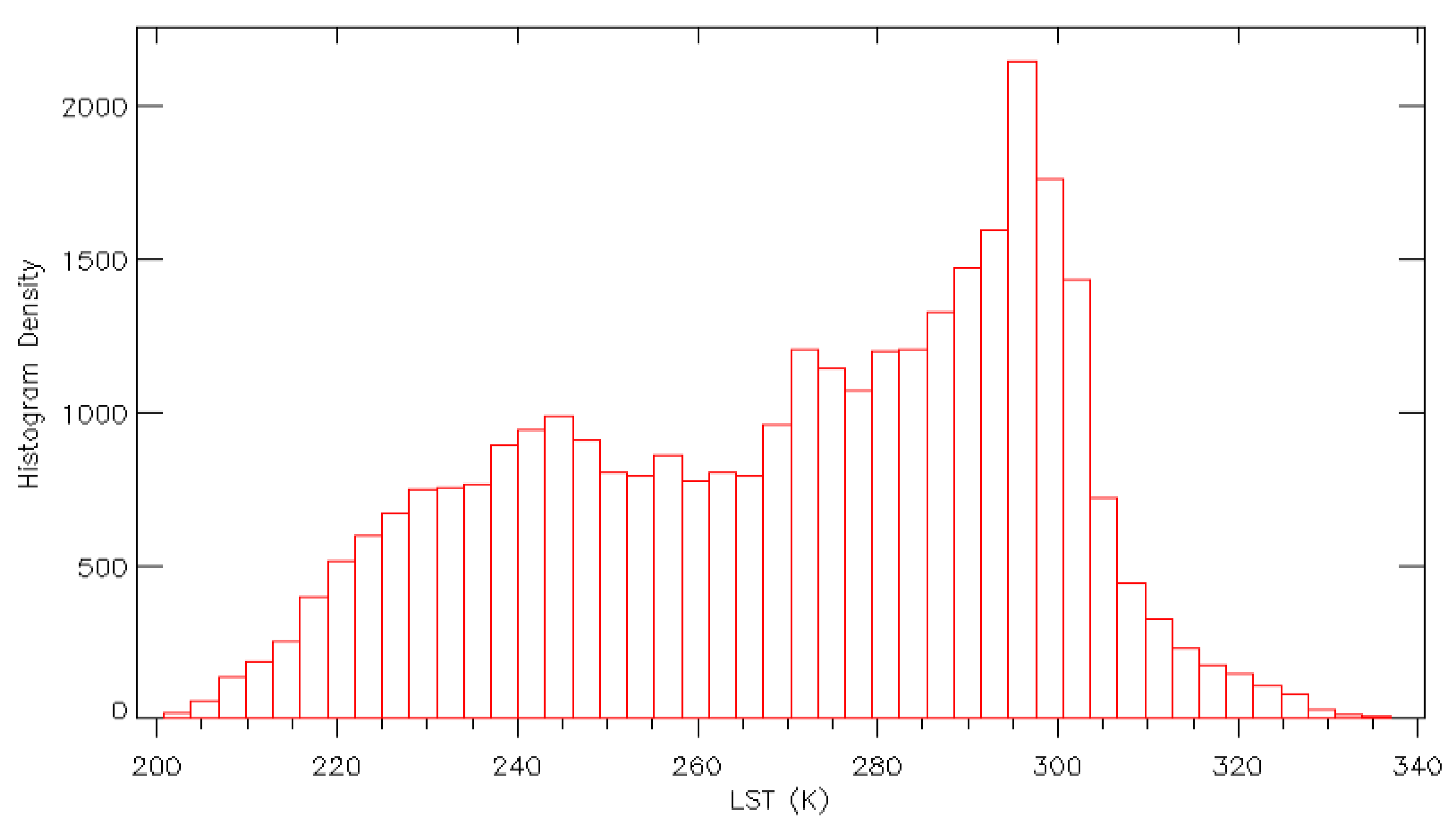
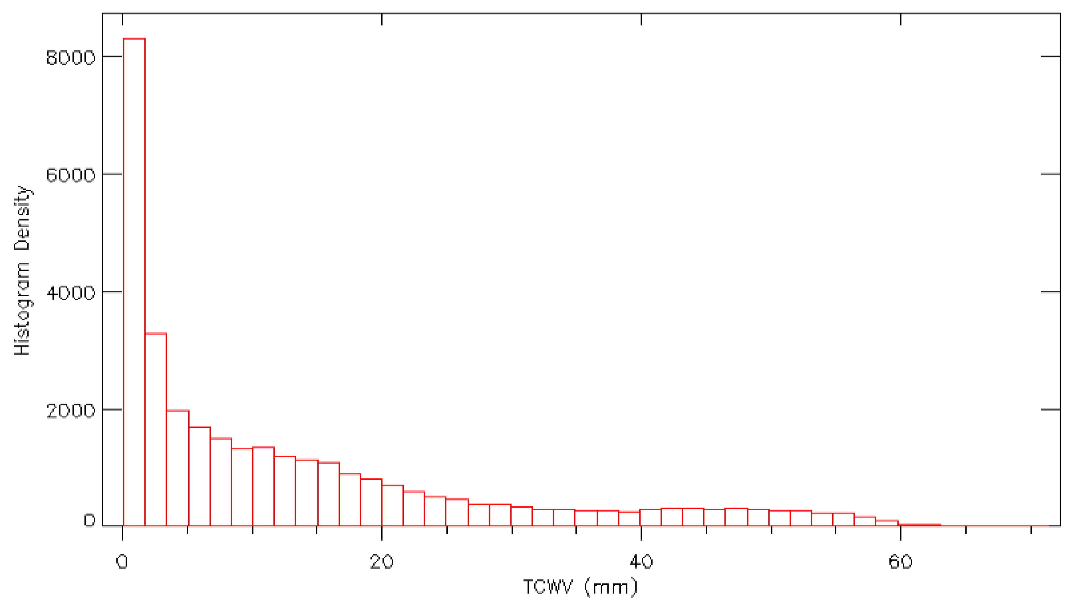
The selection process means that the location of the profile within the 5 × 5° grid cell is not the same each time and therefore the distribution across the land surface is, while representative, not regular. The whole range of selected profiles were assessed to ensure that the parameters being selected were representative of a broad range of realistic conditions. See the distributions of the LST and the TCWV in
Figure 2 and
Figure 3.
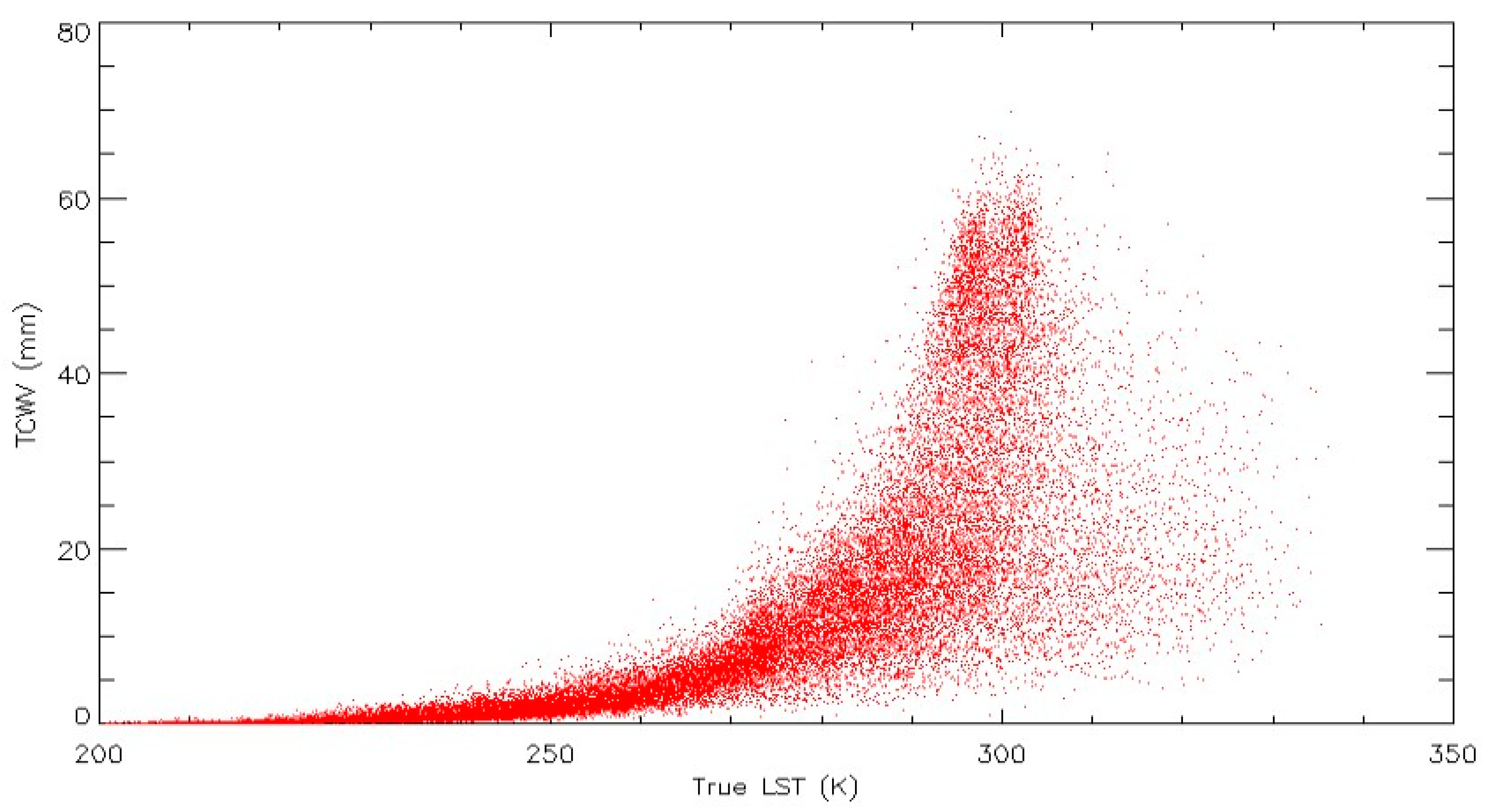
Furthermore, to check for unphysical combinations of LST, and these parameters are analyzed together, see
Figure 4. The LST and TCWV show expected correlations without significant anomalies across the database.
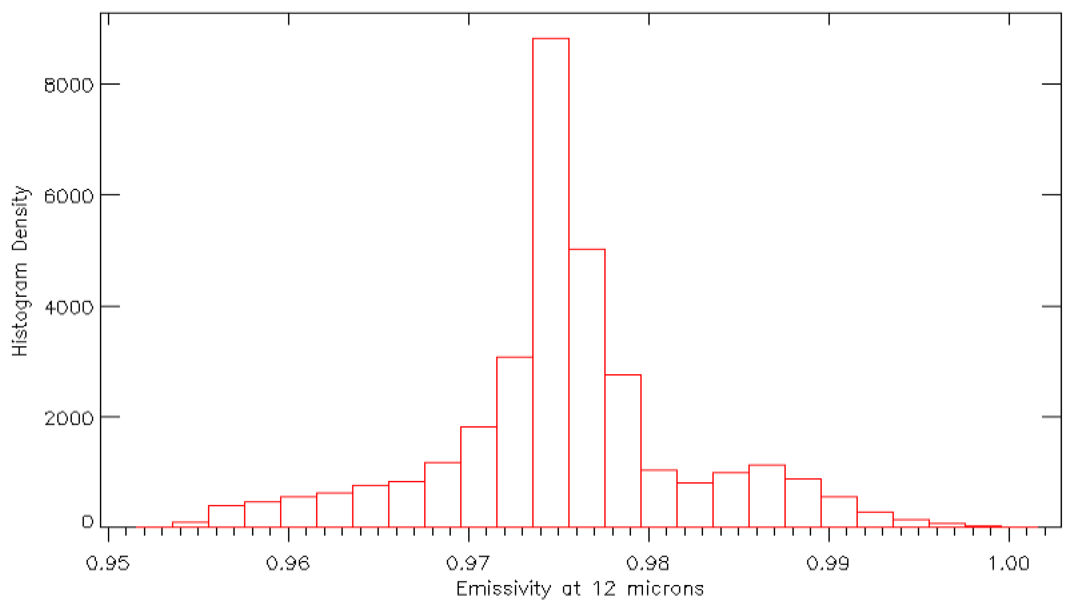
The second stage of processing involves emissivity from either CAMEL or TELSEM. The latitude and longitude information at the locations selected from the ERA5 data is used to find the corresponding emissivity in both cases. In the case of CAMEL, the emissivity data has a higher resolution than the 0.25° ERA5 data. The LSE data are averaged in a 0.25° cell centered on the ERA5 profile location. This is performed to ensure the LSE is representative at the scale of the ERA5 data being used. The distribution of these LSE values across the database is shown in
Figure 5. TELSEM does not need to be spatially averaged as it is at the same resolution as the ERA5 profile data.
For the selection database the LSE values provided are given a random offset from the truth from a Gaussian distribution generated from climatology data. This ensures that the values are representative of the potential prior knowledge of the observation without providing an unrealistically high level of knowledge.
The surface and atmospheric parameters are input to the RTTOV forward model along with the various sensor Instrument Spectral Response Functions (ISRFs). RTTOV then yields the BTs for each sensor for the given simulated truth; these BTs are the simulated TOA observations for each sensor.
As biome is a key parameter on which to assess the performance of the various algorithms, it is important to understand the correlations between the biomes and the parameters of LSE and TCWV. In this study the ATSR Land Surface Temperature Biome Classification V2 (ALB-2) is used as the biome map provided with the TIR dataset. The ALB-2 biome map was specifically used here as it takes account of the main bare soil classes where emissivity values are highly variable [
23]. This is important as the algorithms that have no-explicit emissivity terms (UOL) must be tested in conditions of large emissivity variation. The use of these biomes ensures that the algorithm is exposed to the full range of emissivity variation in the same manner as the algorithms that directly assimilate emissivity.
Table 3 shows the mean and standard deviations for LSE and TCWV for each of the biomes used with more than 5 pixels per day. Biomes 1, 2, 5, 13 and 26 were selected as the most useful biomes to evaluate the impact of TCWV on a retrieval, with biome 5 showing the greatest sensitivity to TCWV with the lowest variability due to LSE allowing for the most independent assessment.
Biomes 15, 21, 22 and 23 show low TCWV variability and large variability in LSE. Biome 15 (sparse vegetation), in particular, is highly variable temporally and biomes 21–23 are associated with impervious surfaces.
2.4. Algorithm Assessment Methodology
Independent assessment requires that the database is split into three different datasets: ’Training’, ‘Testing’ and ‘Selection’. ‘Training’ is the subset used for determining coefficients in empirically derived algorithms, for any other form of algorithm tuning, and/or as a training dataset in a supervised NN optimization (or similar). ‘Testing’ is the subset used to get a (statistically) independent assessment of the algorithm developed using the training. ‘Selection’ is the subset is provided without simulated truth values (TCWV or LSE), and with fields sufficient only to derive LSTs for each “blind” matchup using the coefficients determined from the training and testing stages. Each of these datasets contains a year of data including 3 days from each month: 5th, 15th and 25th. The selection subset is used to carry out the assessment of the algorithms performance.
This splitting of the database is performed so that the algorithms can first be developed on the ‘Training’, then refined on the ‘Testing’ dataset, whilst still leaving the ‘selection’ dataset as a third independent dataset for unbiased assessment. This is important as the refinement on the ‘testing’ dataset allows the algorithms to be tuned without an overreliance on a single year of data.
The selection data does not contain the true TCWV or LSE values. Therefore, the TIR algorithms must be given an alternative and consistent source of LSE and TCWV. Climatology data are used as this source, with 3 years of ERA-Interim profile data and 3 years of CAMEL data used to generate climatologies at 0.25° resolution. The variability of the water vapor in the grid cell can differ strongly from the profile selected by the mean TCWV match. This is also true for the emissivity from the CAMEL dataset. Therefore, for each grid cell the standard deviation of the TCWV and the emissivity per month are calculated. These values are taken as the nominal range in which the prior information of the surface and atmosphere could vary. Concerning the MW algorithms, TELSEM provides climatological means and standard deviations at 0.25° resolution, so these values are taken as nominal range.
Algorithms that require input emissivity are supplied with a value for emissivity equal to the true emissivity from the CAMEL/TELSEM dataset perturbed by a randomly generated value within the range of the climatology standard deviation for emissivity, whilst algorithms that do not explicitly assimilate emissivity vary through the changes in biome. The same process is repeated for the TCWV and the TIR algorithms, where the input TCWV value is equal to the true TCWV from the ERA5 dataset perturbed by a random value in the range of the climatology standard deviation for TCWV.
The median bias for the sensor is calculated as LST minus Tskin. A low bias is the key criteria. The regular grid results in oversampling of the northern and southern latitudes, this can over emphasize the performance over polar regions. However, the analysis is focused on key biomes to assess the performance which mitigate the impact of the oversampling. The precision is calculated as the robust standard deviation of the bias (LST sensor—Tskin) across all pixels.
During the process of running the algorithms the input parameters of emissivity, TCWV and observed BTs are perturbed by a set amount to gauge each algorithm-sensor retrieved LST sensitivity to these parameters. Each parameter is given a set of 6 perturbations to cover a full range of variation. This means that each pixel produces n + 1 LST values, where n is the combined number of perturbations from LSE, TCWV and BT. This sensitivity assessment is conducted for the selection dataset for each perturbation.
The perturbations for BT are ±0.1, 0.5 and 1.0 K. These values are selected to simulate the potential range of Noise Equivalent delta Temperatures (NEdT) and Absolute Radiometric Accuracy (ARA) variations across different instruments.
The perturbations for emissivity are ±0.01, 0.02 and 0.03. These values are selected based on analysis conducted during both the generation of the benchmark database and the climatology. The maximum perturbation (0.03) even at 12 µm is far larger than the standard deviation in each grid cell. Based on the distributions from the climatology and benchmark database generation, a 0.01 minimum perturbation is selected to stand out from the random variation within the climatology standard deviation from each pixel. A maximum of 0.03 emissivity perturbation is selected as being the upper most variation seen with statistical significance within the climatology dataset. The subtler variations in the LSE are captured in the variation within the biomes.
The perturbations for TCWV are ±0.1, 0.25 and 0.5 cm. The perturbation is applied to the knowledge given to the retrieval. The true profile is unperturbed, but the information given to the retrieval is perturbed to assess the sensitivity of the retrieved LST to a change in the TCWV value given to it. These values are selected based on analysis conducted during both the generation of the benchmark database and the climatology. Most of the split-window algorithms have banded coefficients based on total column water vapor, so it is important to select values that whilst realistic have a chance to incur a change in which a different band coefficient is utilized in the retrieval. 0.5 cm is selected as a maximum value as it represents a large change, seen in only few grid cells but also ensures a coefficient change in a statistically significant amount of methodologies.
3. Results
Thermal Infrared
Considering the median bias across all the tested algorithms, the UOL and GSW algorithms provide the closest match to the simulated truth across most sensors, these biases for all algorithms can be seen in
Table 4. QSW, ELA and OE have biases of similar order across the sensors. ELA shows biases in excess of 2 K in southern America, southern Africa, southern Australia and Europe. The scale and magnitude of these biases excludes this algorithm from being used in these regions. OE presents a more random distribution of biases globally due to a strong dependence on the prior climatology data being used in the retrieval.
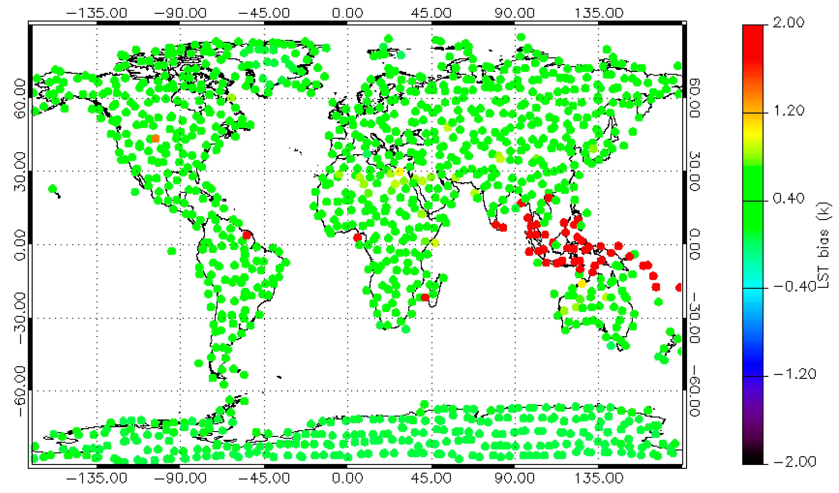
GSW has a high consistency across the whole selection dataset closely followed by UOL. UOL and ELA present low standard deviations but have reduced performance at a global level. QSW has a larger bias in South-East Asia with underestimates of 1.5 K and above. This is highly specified to this region but presents a problem for global applicability; see
Figure 6. OE and SYN perform significantly worse than the other algorithms in terms of precision with large standard deviations across all regions except the Antarctic.
UOL, GSW, QSW and ELA are all generally applicable to split-window sensors and have proven operational heritage. OE is extremely generic, allowing for any permutation of channel and sensor combination. SYN is applicable to any split-window sensor but the lack of banding limits its global applicability.
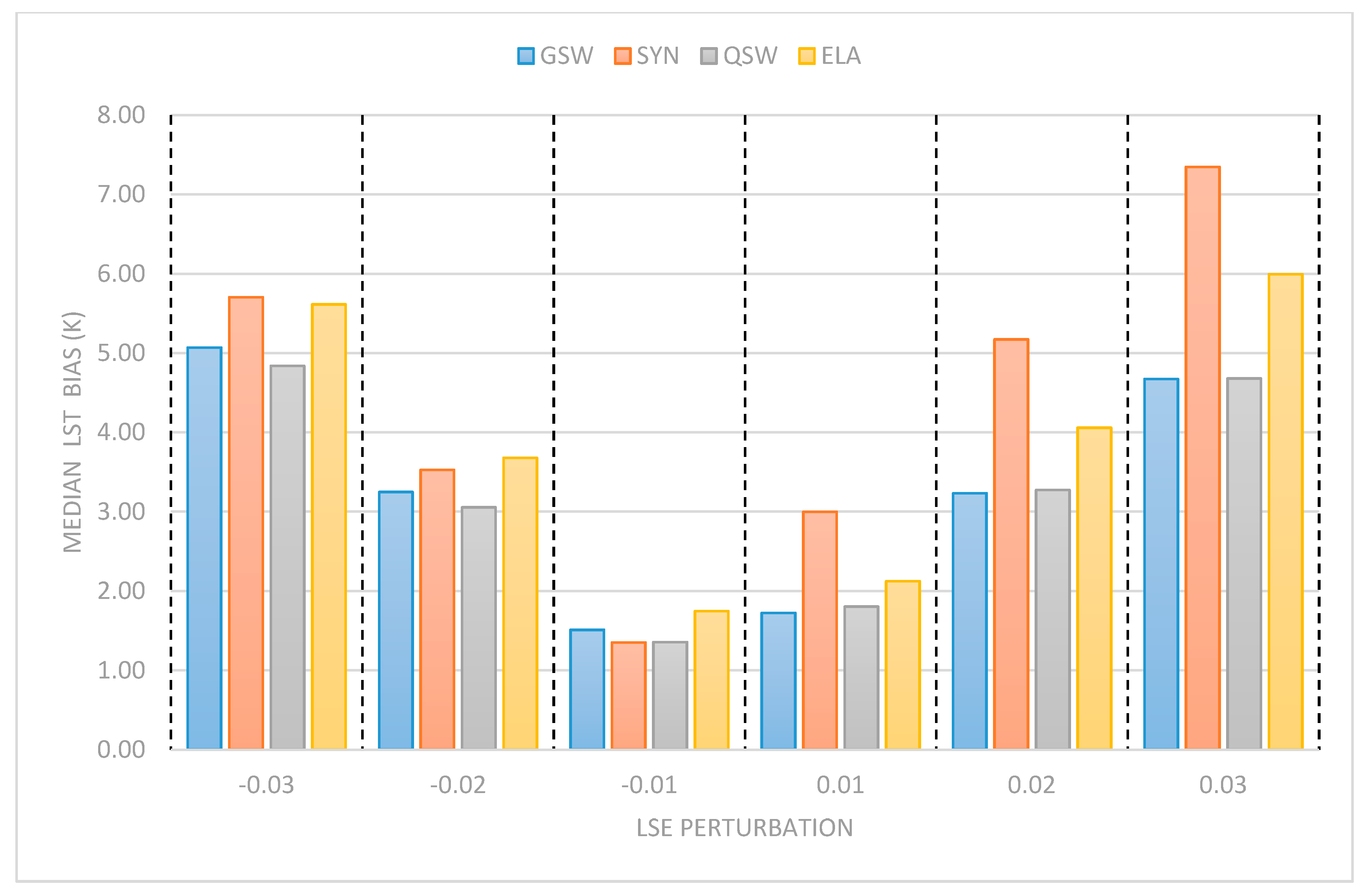
The QSW, GWS, SYN and ELA algorithms benefit from improved estimates of emissivity used in the retrieval.
Figure 7 shows the impact when an offset is applied to the LSE provided to algorithms that explicitly ingest it (OE is not included as it draws its LSE prior from climatology). There is an expected increase in the median bias across algorithms when provided with progressively inaccurate LSE data. At perturbations of ±0.01 LSE, there is 1–2 K impact on the LST bias. This high impact of LSE is expected and it is important to note that the perturbation above 0.01 are not representative of operational normality but are included to test across the range of extremes.
As not all algorithms use LSE explicitly, a more consistent and physically realistic metric is used to compare their performance across different biomes that have within them a variety of surface compositions and atmospheres.
Figure 8 shows the performance in the testing database of all TIR algorithms across five different biome types: three vegetative and one bare soil and one permanent ice. These five biomes cover deciduous and coniferous trees, as well as lower level or sparse vegetation. The bare soils biomes are impervious surfaces which occur under very different climatic atmospheric conditions; see
Table 3 above. For reference the LSE standard deviations inside these biomes are under ±0.01 except biome 15, which has a standard deviation of 0.011. The UOL algorithm is sensitive to LSE through the biome coefficients and biome 15 and presents 0.5 K bias with a LSE standard deviation of 0.01. This shows less sensitivity than the direct LSE algorithms, but still shows sensitivity to real surface LSE conditions.
GSW and QSW are fairly consistent across the biomes, with the exception of biome 23 where the GSW shows a small increase in median bias. This biome is bare soil with a low level of atmospheric water content; therefore a possible explanation for this is that the land/atmospheric interactions are not being correctly separated out in the retrieval. ELA has consistently poorer performance than the GSW, QSW and UOL algorithms, especially in the low water vapor permanent ice biome (27), where the bias is very large. SYN has a large LSE sensitivity and shows the largest biases of the SW algorithms by over 1 K in three of the five test cases. Its performance is markedly improved, however, in biome 27. SYN has extremely strong TCWV-dependent biases, with large biases in both very dry and very wet atmospheres. The magnitude of the biases correspond strongly with patterns of TCWV and regions of bare soil due to the lack of banding. OE has large outliers in some regions and seems particularly sensitive to regions on the land/sea boundary. The biome information shows OE performs very well over most biomes, but struggles in regions with both very high or very low water vapor content as well as those with low emissivity.
Considering the median biases, of all the tested algorithms, the NNE_A algorithm provides the closest match to the simulated truth with a bias of-0.11 K. (
Table 5). NN_A performs well for the whole database except a larger bias in the high latitudes. These Northern latitudes are regions where the LSE can have a relatively large variability, typically related to the presence or absence of snow, and the NN_A, not having LSE as inputs to further constrain the inversions, performs poorly. LRE_37 and NNE_37 have small biases over much of the globe but performance is significantly reduced in high latitude forests. This is possibly related again to the large LSE variability of boreal forests. Even with LSE is an input, the perturbed LSE can substantially differ from the prior, resulting in large LST biases. LR_37 has very poor performance in all bias metrics, which is not surprising given the use of a single channel and no input LSE. The largest biases occur in the Antarctic and excluding this region noticeably lowers the overall LR_37 bias.
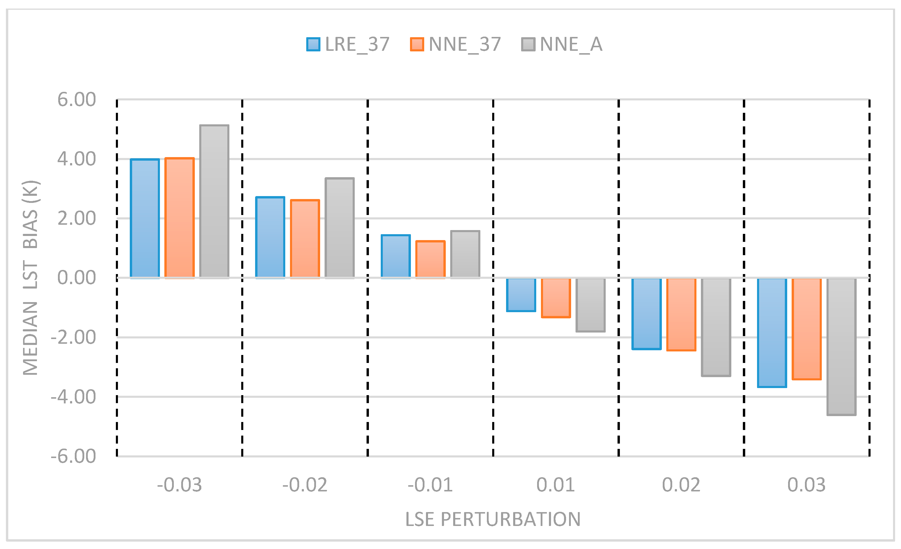
In terms of precision, the methodologies without emissivity (LR_37, NN_A, and LR_A) have very large standard deviations at the global level with values of between 4 and 12 K. LRE_37, NNE_37 and NNE_A have substantially lower standard deviations globally, between 2 and 6 K, but all three methods have large uncertainties in the Antarctic and northern latitudes as commented above. The constraint in the standard deviations is likely due to the additional information of the LSE, with each of these three algorithms having high sensitivity to LSE perturbations, as shown in
Figure 9.
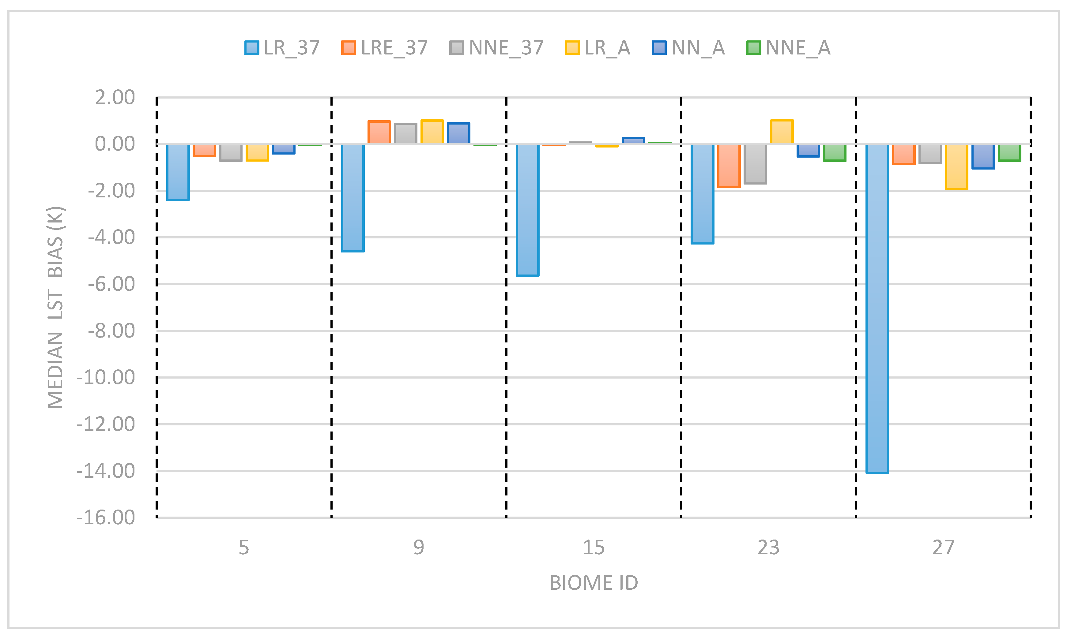
LR_37 has a significantly larger bias in the bare soil biomes (see
Figure 10). NN_A and NNE_A exhibit lower and more consistent biases across the key biomes. It is important to contrast this result with
Figure 9. The high sensitivity seen by these algorithms is due to the large change in LSE used to test extremes. Under more realistic subtle variations in the LSE, like those that occur within and between biomes, the algorithms, with the exception of LR_37, show much better performance.
4. Discussion
In this study, a wide range of performances between different sensors and retrieval methods are observed. Algorithms in the TIR typically present biases of under 1 K and precisions of less than 2 K across sensors, with some notable exceptions that are discussed in the following section. In the MW, biases again are typically of the order of 1 K or less, but there are significantly higher standard deviation of approximately 5 K in many products.
The UOL algorithm is consistently in the top three performing algorithms with median biases (retrieved LST—simulated truth LST) of between 0.07 and 0.16 K across all sensors. The global distribution of the biases is consistent, with only a few regions being notably poorer; those being parts of northern Canada and the Sahara across all three TIR sensor tests. In Canada, these biases correspond with potential ice or snow cover and potentially show a mismatch between the biome information used and the emissivity from the CAMEL dataset. These biases range between 1.2 and 4.6 K. The larger biases in the Sahara could be due to the impervious materials in this region, possessing more extreme LSE values within the UoL biomes. These two regions highlight two potential issues in the UOL algorithm. Firstly, the biome dependence is very high, meaning that a misclassification in the biome data used can result in large biases. A key improvement would be to switch to the Land Cover CCI classification, which is a more recent and temporally dynamic product, and to make use of Snow Cover CCI data in future implementation Secondly, the biome metrics showed that the algorithm is sensitive to the TCWV and LSE but does not have the same level of dependence as the algorithms that directly assimilate LSE and TCWV. Whilst the breakdown of the coefficients by biome is a strength of the methodology (allowing increased resolution in coefficient space to more accurately tailor the coefficient to the true surface resulting in low global biases), it also gives rise to the potential of overfitting. However, the improvements in fitting, demonstrated by lower regional median biases observed in this study outweigh the higher sensitivity introduced.
The UOL algorithm also performs consistently with average standard deviations of between 0.65 and 0.97 K for the whole database. There are no strong geographical trends in the standard deviations. The algorithm is limited to split-window instruments but is generically applicable to any such instrument. The method itself is extremely fast and can be implemented at both an operational and climate dataset level. Its low standard deviation for instruments such as AATSR, SLSTR and MODIS make it a good candidate for climate studies and therefore the merged CDR product. However, the reliance on high instrument accuracy would impair its performance for sensors such as AVHRR. Key areas to improve would be in the biomes used to band the coefficients, additional work being required for biome work with GEO sensors due to the coarser resolution grids. There is potential for improvement through the introduction of temperature-dependent coefficients, an area currently under investigation.
The GSW algorithm is consistently in the top two performing algorithms with median biases of between −0.21 and −0.1 K between the retrieved and simulated truth LST values across all sensors. There is a good consistency over different global regions with marginally poorer performances over impervious materials. GSW is geographically dependent, based on the emissivity. These LSE influences are well constrained to regions of impervious surfaces which represent a relatively small fraction of the land surface area, so the overall performance of the algorithm maintains a high standard. The algorithm is limited to split-window instruments but is generically applicable to any such instrument. The method itself is extremely fast and can be implemented at both an operational and climate dataset level. Key areas to improve would be in the emissivity estimates given to the retrieval.
The QSW algorithm has consistently good performance with median biases of between −0.25 and −0.09 K between the retrieved and simulated truth LST values across all sensors. There is a good consistency over different global regions, except that the bias is higher in south East Asia across all sensors. This regional impact is very large and not seen in other algorithms. If this region is excluded from the analysis the QSW algorithms, the standard deviation at the global whole database level falls from between 1.25 and 1.28 K to between 0.4 and 0.45 K, which is comparable to or better than GSW. The anomaly in South East Asia, seen in
Figure 6, is only seen in the testing dataset. The datasets are drawn from 3 years: 2013, 2014 and 2015. According to the protocol specified the algorithms are trained on 2015, refined on 2014 and independently tested on 2013 data. 2015 is an El-Nino year, during which the region with larger biases was strongly affected [
45]. It is possible that this algorithm is sensitive to the changing conditions seen in this area during that time, in particular the very high water vapor load in the atmospheric column would be amplified by the quadratic term. However, it would require comparison with in situ data and observations to confirm this. This also highlights a limitation of using a single year as the testing set as it is difficult to remove the impacts of inter annual variations that might lead to anomalous results. This will be further investigated in a future study.
The broader emissivity issues can be improved through the assimilation of more accurate emissivity data. The algorithm is limited to split-window instruments but is generically applicable to any such instrument. The method is extremely fast and can be implemented at both an operational and climate dataset level. Key areas to improve would be in the emissivity estimates given to the retrieval as well as an exploration of the potential sensitivities to haze/aerosols and fires that can result from shifting El-Nino influences, studies looking into these improvements have already shown significant impacts [
46].
The ELA algorithm performs well with median biases of between 0.23 and 0.54 K between the retrieved and simulated truth LST values across all sensors. However, it is usually in the bottom two performing of the split-window algorithms. There is poorer consistency over different global regions, with large variations over impervious surfaces that are likely linked to emissivity. There are also biases across North America and Western Europe in the AATSR data, but the source of these biases is currently unclear. The ELA algorithm has a larger standard deviation than both GSW and UOL at the global whole dataset level of between 0.54 and 0.98 K. This large standard deviation reduced when looking at the mean and median standard deviations for each of the grid cells, 0.45 to 0.9 K. The presence of these anomalies in a particular sensor demonstrates a potential issue with the generality of the algorithm when applied to harmonized datasets including multiple sensors.
The ELA algorithm is highly sensitive to the input parameters showing the highest LST sensitivities to changing emissivity and water vapor in the MODIS data. The biases relating to impervious surfaces require improved emissivity estimates. The algorithm is limited to split-window instruments but is generically applicable to any such instrument. The method is extremely fast and can be implemented at both an operational and climate dataset level. Key areas to improve would be in the emissivity estimates given to the retrieval as well as sensor-specific tuning to investigate the biases in AATSR applications.
The SYN algorithm performance varies significantly between sensors, with median biases of between 0.04 and 2.6 K between the retrieved and simulated truth LST values across all sensors. There are strong geographical variations with correlations between mean biases and the magnitude of TCWV. SYN has significantly larger standard deviations in all sensors except AATSR with global standard deviations between 1.5 and 9 (MODIS) K, which are strongly driven by the TCWV. This is reduced when looking at median standard deviations for each of the grid cells, 0.6 to 4 (MODIS) K. SYN presents very large TCWV-dependent biases due to the lack of banding. Although SYN is applicable to any split-window sensor the lack of banding limits its global applicability. The algorithm is limited to split-window instruments but is generically applicable to any such instrument. The method its self is extremely fast and can be implemented at both an operational and climate dataset level. The key area to improve SYN would be banding to incorporate either biomes or TCWV as a coefficient parameter.
The OE algorithm performs consistently with median biases of between 0.13 and 0.16 K between the retrieved and simulated truth LST values across all sensors. There is a good consistency over different global regions. However, where biases are present, the magnitude of these differences is very large. This is primarily due to the use of climatology data in the prior information given to the OE method. Due to the use of only two channels, the OE is heavily reliant on the prior information. The climatologies, whilst broadly representative, have differences from the simulated truth in order to be a fair and representative testing environment. The geographical distribution of the large biases is sporadic and almost random in nature. This is because the differences are not physically or environmentally driven, rather they relate to the differences between the climatology and the database, and therefore can be subject to gridding artefacts from land-sea masking. This is seen in the standard deviation where OE has the largest standard deviation in this study at the global whole dataset level of between 5.9 and 6 K.
Across the MW algorithms, those based on a non-linear regression implemented by a NN provide the best global consistency in terms of both bias and standard deviation. This indicates that the mapping between BTs, LST, and LSE cannot be properly characterized by a simpler linear regression. Additionally, using all of the available channels provides a marked improvement when compared to the methods that use only the 37.0 GHz vertically polarized channel. This confirms that having the additional information about the surface and atmosphere states provided by the remaining channels is useful to further constrain the inversion problem. The introduction of LSE as an input improves the regional performance particularly in the Northern Hemisphere. The large LSE variability in some of the regions of the Northern Hemisphere makes the inversions difficult due to the relatively large dependence of the BTs on the LSE. These difficulties are partly mitigated by having pre-calculated seasonal LSE values available to further guide the retrievals. Assessing all of the numeric metrics, the NNE_A algorithm has both the lowest bias and standard deviation.
5. Conclusions
In conclusion, this study has constructed a novel and robust database and methodology for the intercomparison and assessment of multiple TIR and MW retrieval algorithms across four different satellite sensors. The database, and breakdown into independent training and testing datasets, has enabled algorithms to be compared without the potential issues of site-specific biases found in in situ validation.
The assessment compared the retrieval performance not only through the mathematical perturbations of the input radiance, emissivity and water vapor, but also by the physically representative biomes at the geographical locations observed. This has enabled this study to capture both the extremes as well as the subtle variations in surface and atmospheric conditions in order to analyze these impacts on the retrieval algorithms. Furthermore, assessments based in realistic biomes allow the surface and atmospheric variables to fluctuate in a linked fashion that is true to the conditions that would be observed by the sensor. The biome-based assessment allowed the results to be analyzed by the occurrence of the biome within nature and thereby weighted the algorithms performance at a global level towards a greater degree of representivity.
This study aimed to determine the optimal algorithms for single-sensor LST products for AATSR, Terra-MODIS, SEVIRI and SSM/I; a CDR for a combined database drawing from AATSR, SLSTR and MODIS; and finally a merged low Earth orbit/geostationary product using data from AATSR, MODIS and SEVIRI. Based on this assessment, the optimal algorithms for use for each sensor/product are:
AATSR: GSW and UOL are both suitable, with biases of −0.19 and −0.07 K and standard deviations of 0.47 and 0.65 K, respectively.
MODIS: GSW and UOL are both suitable, with biases of −0.1 and −0.16 K and standard deviations of 0.48 and 0.97 K, respectively.
SEVIRI: GSW is the most suitable, with a bias of −0.21 K and a standard deviation of 0.48 K. Whilst UOL is close in performance, the high temporal resolution of SEVIRI leads to improved estimates of the explicit LSE as it is broadly invariant over time.
SSMI: NNE_A is the most suitable algorithm for use with SSMI, with, by far, the best performance in terms of the bias (0.11 K) and with a standard deviation of 2 K, marking it as the most consistent of the MW algorithms.
Long term: GSW due to consistent performance on AATSR and MODIS.
Combined GEO/LEO product: GSW due to consistent performance on AATSR, MODIS and SEVIRI.
QSW provides another option for further investigation with good performance showing biases of −0.25 K or lower across all 3 TIR sensors and standard deviations of 1.3 K or lower. However, regional anomalies need to be traced and explored before this algorithm can be considered for global analysis.
Throughout this study, the method and structure of the benchmark database has provided a robust and adaptable environment in which algorithms can be fairly compared and assessed; however, this study has highlighted areas in which further study would be of great benefit. Specifically, the database will benefit from extending over multiple years to remove the impact of interannual features. Furthermore, the results of this study have opened the algorithms themselves up for further investigation, particularly with respect to the banding of retrieval coefficients by temperature and water vapor.
Despite these areas, which warrant further investigation, and the improvements suggested, the results of this study provide a statistically robust and independent assessment of multiple algorithms and provide a guide through which the ESA CCI can implement the optimal algorithms to produce consistent and traceable LST data across multiple sensors.

 ,
, 


