The Potential of ICESat-2 to Identify Carbon-Rich Peatlands in Indonesia

1
RSS—Remote Sensing Solutions GmbH, Dingolfinger Str. 9, 81673 Munich, Germany
2
Department of Biology, Ludwig-Maximilian-University Munich, Großhaderner Str. 2, 82152 Planegg-Martinsried, Germany
*
Author to whom correspondence should be addressed.
Remote Sens. 2020, 12(24), 4175; https://0-doi-org.brum.beds.ac.uk/10.3390/rs12244175
Submission received: 30 October 2020
/
Revised: 15 December 2020
/
Accepted: 16 December 2020
/
Published: 20 December 2020
Abstract
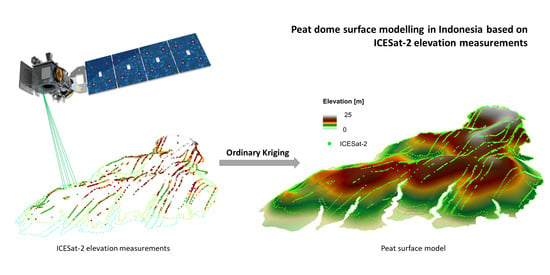
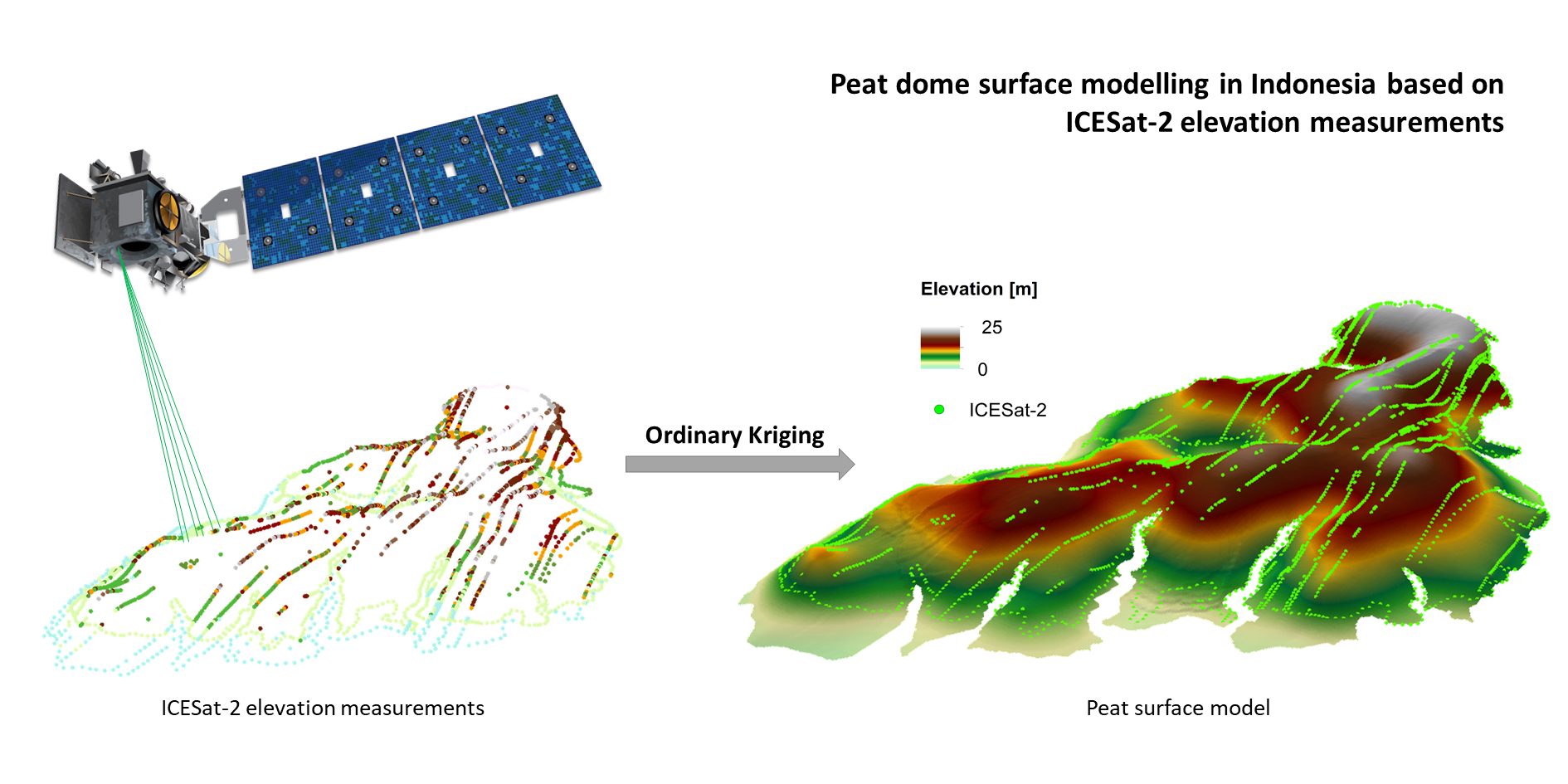
:Peatlands in Indonesia are one of the primary global storages for terrestrial organic carbon. Poor land management, drainage, and recurrent fires lead to the release of huge amounts of carbon dioxide. Accurate information about the extent of the peatlands and its 3D surface topography is crucial for assessing and quantifying this globally relevant carbon store. To identify the most carbon-rich peatlands—dome-shaped ombrogenous peat—by collecting GPS-based terrain data is almost impossible, as these peatlands are often located in remote areas, frequently flooded, and usually covered by dense tropical forest vegetation. The detection by airborne LiDAR or spaceborne remote sensing in Indonesia is costly and laborious. This study investigated the potential of the ICESat-2/ATLAS LiDAR satellite data to identify and map carbon-rich peatlands. The spaceborne ICESat-2 LiDAR data were compared and correlated with highly accurate field validated digital terrain models (DTM) generated from airborne LiDAR as well as the commercial global WorldDEM DTM dataset. Compared to the airborne DTM, the ICESat-2 LiDAR data produced an R2 of 0.89 and an RMSE of 0.83 m. For the comparison with the WorldDEM DTM, the resulting R2 lay at 0.94 and the RMSE at 0.86 m. We model the peat dome surface from individual peat hydrological units by performing ordinary kriging on ICESat-2 DTM-footprint data. These ICESat-2 based peatland models, compared to a WorldDEM DTM and airborne DTM, produced an R2 of 0.78, 0.84, and 0.94 in Kalimantan and an R2 of 0.69, 0.72, and 0.85 in Sumatra. The RMSE ranged from 0.68 m to 2.68 m. These results demonstrate the potential of ICESat-2 in assessing peat surface topography. Since ICESat-2 will collect more data worldwide in the years to come, it can be used to survey and map carbon-rich tropical peatlands globally and free of charge.
1. Introduction
In the context of climate change and recurrent large-scale fire disasters, the accurate determination of carbon contents of vegetation and soil in terrestrial ecosystems is becoming increasingly important. While carbon-rich peatlands only cover 3–5% of the earth’s surface, they store about 30% of all terrestrial soil carbon [1].
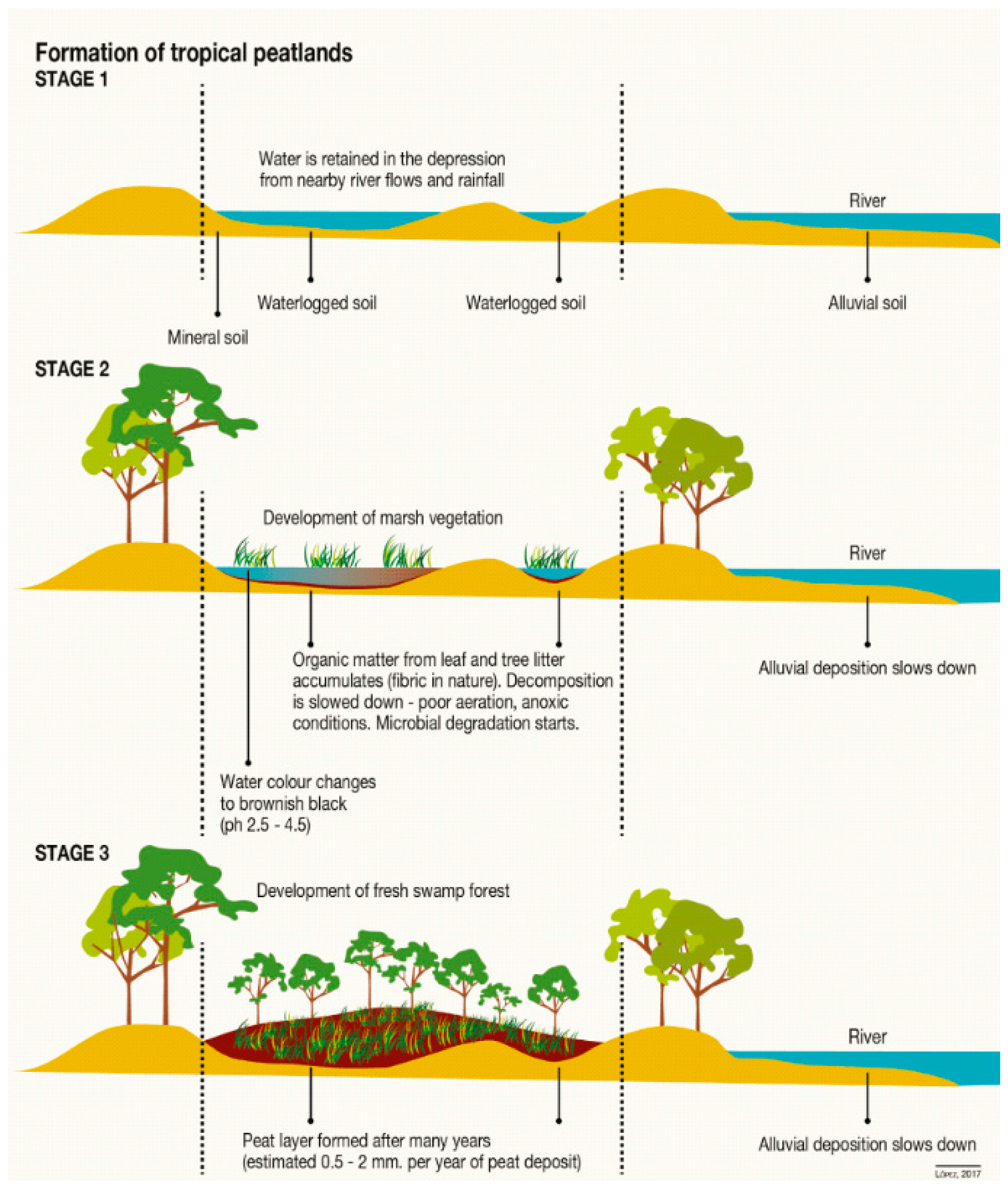
Indonesian peatlands developed over the past thousands of years when sea level rose to today’s level. Plant debris accumulated under waterlogged conditions in natural sinks such as lakes or alluvial floodplains and formed convex domes of up to 20 m thickness and up to 100 km width (see Figure 1) [2]. This ombrogenous type of peat is most widely found in Southeast Asia, and it carries high carbon contents. Peat swamp forests that grow on top of peatlands form and protect the peat layer. Due to deforestation, logging, and drainage, 80 million ha of forest were lost in Southeast Asia between 2005 and 2015. Indonesia accounts for approximately 62% of this forest loss [3].
Indonesia has the largest known peat reservoirs in Asia, with an estimated extent of 16.8–27.0 million ha of peat [5,6,7]. The carbon stored in Indonesian peatlands alone could be up to 55–75 Gt, which equals 25% of the carbon stored in all tropical forests worldwide [8,9,10]. The carbon stored in the aboveground biomass of the forests growing on peat can be up to 300 tons per hectare (t/ha), with an average of 70–150 t/ha [5]. Estimates of peatland extent and volume as well as the carbon store are still speculative and show a wide range in the literature [11,12]. Many peatlands have been damaged by wildfires, legal and illegal logging, and unsustainable land use [13]. Recurrent wildfires lead to huge emissions of CO2 and other greenhouse gases by peat combustion, while excessive drainage leads to continuing peat decomposition and subsequent emissions [14,15].
Besides the uncertainty of peat area extent in Southeast Asia, peat layer and carbon stock volumes are challenging to determine accurately. The most precise method for measuring peat thickness is by collecting in situ data using peat corers. However, peat coring is difficult, time-consuming, and expensive because many peatlands are located in remote areas with poor accessibility. Peat swamps are flooded several months per year, and covered by dense forest, making them almost impossible to access.
The spatial extent of peat was already mapped by multispectral satellite remote sensing [16]. Assessing the volume of the peat layer by remote sensing is more difficult. One approach is to identify raised peat domes using airborne and spaceborne LiDAR instruments and radar (SAR) satellites [13,17,18,19,20,21]. These sensors can penetrate the dense forest cover and create a digital terrain model (DTM) of the peat soil surface beneath the vegetation cover. Several authors [7,22,23,24,25] found a correlation between the height of the biconvex peat dome surface and the thickness of analyzed peat domes in Indonesia. The surface and depth information, in combination with drillings, allow the calculation of a 3D model of the peat layer and thus the estimation of the carbon stored in the peat layer [7,11,22].
Measurements with airborne LiDAR are more accurate than spaceborne LiDAR, but it is costly to fly airplanes over large and remote areas in Indonesian topical forests. With the ICESat-2/ATLAS instrument, for the first time, there is a spaceborne LiDAR instrument available that collects massive data globally and is distributed at no charge. The objective of this study was to investigate the applicability of this new sensor to identify carbon-rich dome-shaped peatlands. To validate the results, we compared the footprint DTM measurements obtained with ICESat-2 to highly accurate airborne LiDAR DTM, which we had available for several study sites in Kalimantan on the island of Borneo [26]. The airborne LiDAR DTM was validated by differential GPS measurements taken in situ. In a second step, we used the ICESat-2 footprint DTM data to generate a wall-to-wall model of the peat surface topography using the geostatistical interpolation [27]. The resulting peat dome surface model was compared to the airborne LiDAR DTM and a highly accurate commercial DTM created by Airbus from the TanDEM-X SAR mission.
2. Materials and Methods
2.1. Study Area
Our study focused on one of the largest and less disturbed peat swamp forest complexes in Indonesia, located in Central Kalimantan. It consists of three peat hydrological units (PHU): Sungai Katingan Sebangau, Sungai Kahayan Sebangau, and Sungai Kahayan Kapuas (from west to east, see Figure 2). The peatlands are ombrogenous and have a peat depth varying from 0.5 to 12 m [13]. Sungai Kahayan Sebangau and Sungai Kahayan Kapuas have been extensively logged and deforested by recurrent fires. In the course of the Mega Rice Project, a resettlement project by the Indonesian Government in the 1990s, large areas were drained through irrigation channels [7]. The damaged forests and drained peatlands became susceptible to fire and frequently burned over the past two decades [28]. The largest peatland, Sungai Katingan Sebangau, contains the Sebangau National Park, an area of almost one million ha of undisturbed peatlands [29]. The forests are largely undisturbed and characterized by dense low pole forest with a canopy height of about 10–20 m and tall peat swamp forests with trees of up to 45 m tall. Furthermore, three PHUs with similar characteristics but located near the coast of Sumatra were analyzed (Figure 2).
2.2. Data
2.2.1. ICESat-2 Data
ICESat-2 was launched in September 2018, carrying a single instrument, the Advanced Topographic Laser Altimeter System (ATLAS). This system is a photon-counting LiDAR that detects sensitivities at the photon level. The sensor operates at a wavelength of 532 nm (green) and a pulse repetition rate of 10 kHz [30]. It uses six beams arranged in three pairs containing a low-energy and a high-energy beam, separated by 90 m in across-track direction. This constellation permits surfaces of low and high reflectivity to be detected [30]. The nominal diameter footprint for each beam is about 17 m [30].
Within the ICESat-2 ATL08 product, photons collected by ATLAS are classified as terrain or canopy and used for computing the final ATL08 parameters. To guarantee continuity, NASA used a fixed segment size of 100 m selected for all parameter calculations (mean, minimum, maximum, etc.) in along-track direction [30]. Each 100 m segment is calculated using five sequential 20 m segments from the ATL03 product, as described in Neuenschwander and Pitts [31].
All derived terrain and canopy height values are defined as absolute heights above the WGS84 ellipsoid [31]. We used all available data from September 2018 through December 2019, which are 43.036 measurements, for the analysis.
2.2.2. EGM2008
The Earth Gravitational Model 2008 (EGM2008) is a spherical harmonic model of the gravitational potential of the earth [32] published by the National Geospatial-Intelligence Agency (NGA). It can be downloaded at [33] for free. We used the EGM2008 to correct the ATLAS terrain height for a potential geoid deviation.
2.2.3. Airborne LiDAR Data
Airborne LiDAR data were collected in 2011 by the Kalimantan Forests and Climate Partnership project funded by Australian aid. The acquisition was flown 800 m aboveground with an Optech Orion M200. The discrete return airborne LiDAR sensor uses a wavelength of 1.064 µm. The data were recorded with a half scan angle of ±22°, a point density of 2.8 points/m2, and a side overlap of 30% [34]. The LiDAR campaign covered an area of 700,000 ha and diverse land cover, including peat swamp forests partly affected by former or recent selective logging, old burn scars, fern, grassland, bushes, and agricultural land [35]. The data were validated based on 942 digital global positioning points. The vertical accuracy lies at 0.18 m for the DTM and the RMSE is 0.09 m [35]. The modeled surface was within a 95% confidence interval of the ground-truth data.
The airborne data for Sumatra were collected in December 2017 with the same flight characteristics and were provided by Badan Restorasi Gambut (BRG).
2.2.4. WorldDEM Data
For additional comparisons, we used the WorldDEM DTM produced by Airbus DS Geo GmbH and provided by BRG. The WorldDEM DTM is based on the WorldDEM product. All WorldDEM products are generated based on X-band radar data acquired from the TanDEM-X mission (2010–2014) operated by Airbus and the German Aerospace Center (DLR). Both radar satellites of this mission operate as a single-pass synthetic aperture radar interferometer (InSAR). Data are acquired with the bistatic InSAR StripMap mode [36].
The DTM contains information about the bare earth elevation, excluding surface features such as vegetation and buildings [36]. With a resolution of 12 × 12 m, the data offer more details than the Shuttle Radar Topography Mission (SRTM, 30 or 90 m spatial resolution) or the ASTER Global Digital Elevation Map (GDEM, 30 m spatial resolution). The vertical relative accuracy of the WorldDEM DTM is 5 m. In flat terrain, the vertical accuracy is improved. The absolute horizontal accuracy lies below 6 m [36].
2.3. Methods
2.3.1. Data Processing
After downloading and preprocessing the product ATL08 (land/vegetation) of ICESat-2 ATLAS, the extracted parameter values were stored in a newly created shape file using the entry latitude and longitude information to generate a geolocated product. The EGM2008 was subtracted from the ICESat-2 terrain height information pointwise to correct for potential geoid deviations [13,37].
Since the airborne LiDAR DTM has a spatial resolution of 1 × 1 m, WorldDEM DTM 12 × 12 m, whereas the ICESat-2/ATLAS covers footprints with a diameter of approximately 20 m [38], the different spatial resolutions need to be taken into account. All WorldDEM and airborne pixels covered by the specific ICESat-2 footprint are identified. The mean elevation of the identified pixels within the ATLAS footprint is calculated and used for further data comparison and evaluation to analyze the same area.
2.3.2. PHU Surface Interpolation Using Ordinary Kriging
To create surface models for the six PHUs based on the ICESat-2 point data, we used kriging, developed by Matheron [27] using R software. Kriging is considered to be one of the most used methods for interpolating nonuniform and irregularly spaced spatial data to model terrain [39,40,41,42,43]. In comparison to other interpolation methods, it can model irregularly spaced data like ICESat-2 measurements. The approach is more sensitive to outliers than other interpolation methods, such as inverse distance weighting since its weights are determined by a variogram. Furthermore, it provides unbiased estimates [44].
Kriging assumes that the direction and distance between points have a spatial correlation. This spatial correlation is used to explain surface variations. The value of a specific location is predicted by estimating a weighted average of the known values in the location’s neighborhood [43]. As a result, the prediction is more accurate at points that are closer to observations and declines with increasing distance. Methods such as simple, ordinary, or universal kriging differ in the consideration of the weighted components. In our study, we used ordinary kriging to interpolate the DTM based on ICESat-2 elevation measurements. Ordinary kriging is considered to be one of the most appropriate methods for interpolating spatial data, because it minimizes the variance of the estimation error [40,43,44]. It is defined as:
where represents the measured values at position i, is an unknown weight for the , defines the prediction location, and N is the number of measurements.
Before applying the interpolation, the dataset was checked for errors potentially resulting from tall vegetation. Tall peat swamp forest subtypes have extensive tree diversity among peat forests and thus some of the highest canopy stratification [5]. We excluded DTM points with a canopy measurement taller than 20 m to avoid errors due to vegetation artifacts.
In addition, the data characteristics were analyzed regarding outliers, a normal distribution, stationarity, and anisotropy before the interpolation [42]. Since ordinary kriging is sensitive to outliers, the datasets were analyzed regarding extreme values. Since the study area is characterized by a flat and smooth topography, no extreme values were found in the data. In addition, the data were analyzed regarding a normal distribution using the Kolmogorov–Smirnov (KS) test before the interpolation. The results of the KS for each of the PHUs showed that the data were not normally distributed in all cases (p-value < 0.05). Therefore, data were transformed to a normal distribution following [45,46,47]. We applied an optimal normalization search function in the package “bestNormalize”. This function tests different transformation functions (Yeo–Johnson, Box Cox, logarithmic, square-root, ordered quantile normalization, and arcsinh) for the specific datasets based on the Pearson P test for normality. The transformation with the lowest P (calculated on the transformed data) was selected. For all six PHUs, the ordered quantile normalization transformation [48] was identified as best and applied to the datasets. Furthermore, the data were tested for stationarity using the autocorrelation function and the augmented Dickey–Fuller test [49,50]. The data were found to be nonstationary.
The best variogram model for each PHU was identified by comparing root mean square error (RMSE) and mean absolute error (MAE). For this purpose, four variogram models (circular, spherical, exponential, Gaussian) were tested [44]. The spherical model outperformed the other three models as indicated by the lowest RMSE and MAE. We tested if the data are anisotropic by computing variograms at different angles (0, 40, 90, and 135) [51] and found no indicators for anisotropy within the data. Thereafter, a grid with 100 × 100 m resolution was defined for storing the kriging surface and ordinary kriging was applied using the fitted variogram [52].
The kriging variance was also estimated for each point within the unit. To model the terrain within the extent of the PHUs, we used a peatland map, derived from historical and recent satellite data to delineate the units. Kriging results were clipped to this extent. Altogether, an area of 21.924 km2 was processed.
2.3.3. Validation
For the validation, we generated a random point layer using the software ArcGIS. The values of the modeled and reference elevations at the random points were extracted and compared in the next step with the airborne LiDAR and WorldDEM DTM data. For this comparison, the coefficient of determination (R2), standard deviation, RMSE, relative RMSE (calculated as the ratio of the RMSE to the mean of the observed variable), and the mean of the terrain heights in meters were calculated.
3. Results
3.1. Peat Surface Topography—Comparison of ICESat-2 and Airborne LiDAR DTM
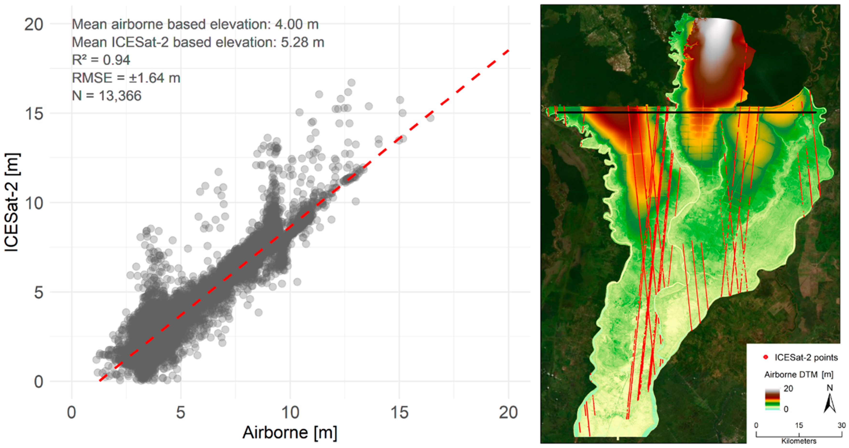
In Kalimantan’s coastal peatlands, the terrain heights vary between 0 and 20 m over a distance of more than 100 km from the shore towards the inland. The highest terrain values were identified in the north of the study area, displayed in white in Figure 3 (map on the right). When comparing ICESat-2 with the highly accurate airborne LiDAR DTM, overlapping datasets showed a strong correlation, as shown in the scatterplot in Figure 3. Altogether, 13,366 ICESat-2 footprints were analyzed within this area. It becomes visible that ICESat-2 tends to overestimate the terrain heights slightly. The mean elevation of the ICESat-2 values lies at 5.28 m, while the airborne LiDAR DTM is at about 4.00 m. The coefficient of determination (R2) reached a value of 0.94, while the RMSE is ±1.61 m. Areas with a vegetation cover below 2 m showed an RMSE of ±1.38 m.
To investigate the origin of this discrepancy in more detail, we analyzed the ICESat-2 DTM measurements in relation to the vegetation cover. A dense forest canopy may prevent the spaceborne LiDAR from reaching the terrain beneath the forest canopy [38]. Extracting and plotting DTM values along various transects covering single ICESat-2 orbits allowed a detailed analysis of the quality of the ICESat-2 dataset regarding any disturbance by vegetation. Transects encompassed dome-shaped ombrogenous peatland covered by peat swamp forests with trees up to 40 m tall, palm oil trees up to 15 m tall, burned bushland and grassland, and almost bare soil in recently established plantations. As expected, the ICESat-2 derived DTM showed a very good correlation with airborne DTM, especially in sparsely vegetated areas. In areas covered by dense peat swamp forests, ICESat-2 DTM showed a divergence of ±6.13 m (RMSE) compared to the airborne DTM. In areas with low vegetation (oil palm, bushland), the accuracy of the ICESat-2 data increased to ±0.70 cm.
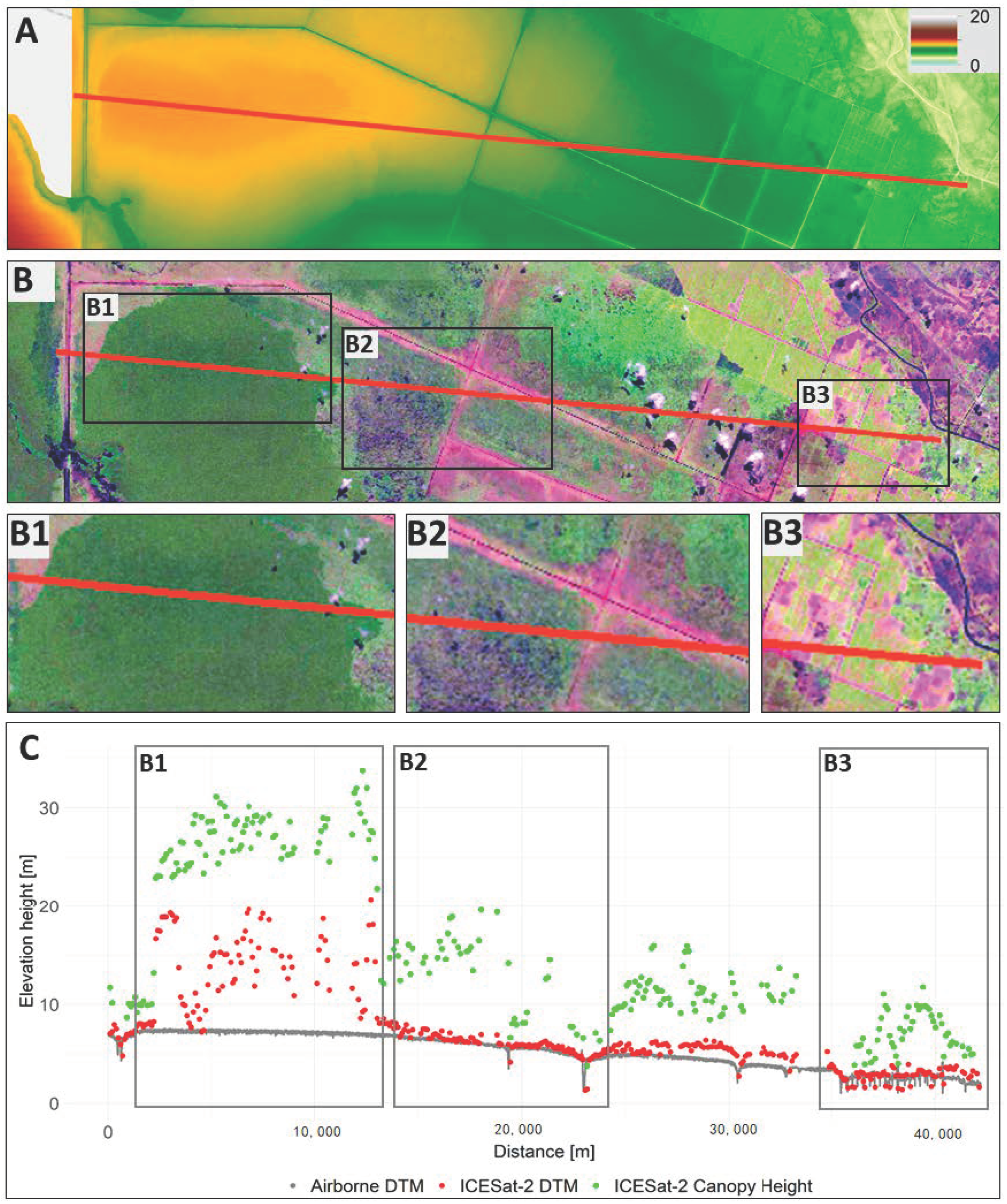
The mean absolute error varied between 5.20 m for dense and tall vegetation and 0.63 m for low vegetation. To illustrate the disturbance of the ICESat-2 DTM by various vegetation types, Figure 4 shows a close up of a north–south transect. The transect is approximately 42 km long and covers tall peat swamp forest, degraded and logged forest, shrubland, and an oil palm plantation. Our own field observations confirmed this classification. In dense peat swamp forests with a closed canopy at approximately 30 m (Figure 4B1), the ICESat-2 DTM has an error of up to 10 m, as determined from the airborne DTM (Figure 4C). In contrast, in areas covered by shrubs and young trees (<15 m, Figure 4B2), the error ranges from 0.1 to 0.9 m. A similar observation can be made in a young oil palm plantation with trees smaller than 10 m, Figure 4B3). The overestimation of terrain height is here in the range of about 0.5 m.
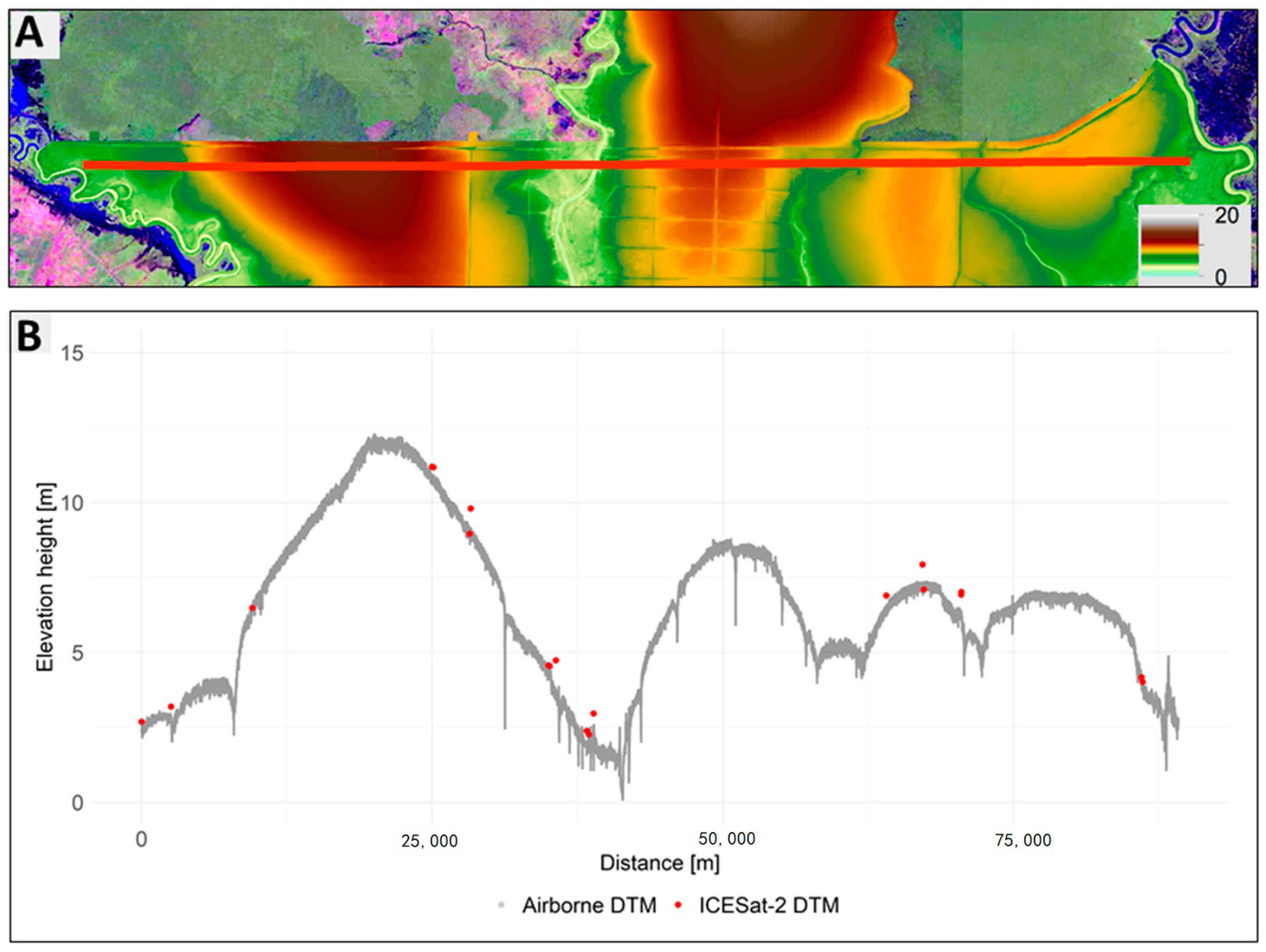
In the next step, we eliminated inaccurate ICESat-2 DTM measurements, which were erroneous due to vegetation artifacts. Figure 5 shows a comparison of the airborne DTM and the ICESat-2 DTM along a transect across four large peat domes (east to west, location shown as a black line in Figure 3). The domes are characterized by a flat topography with an elevation change of only 9 m across a distance of 88 km. The raised peat domes are clearly visible in the airborne DTM (gray line in Figure 5B). Because ICESat-2 orbits are recorded from north to south, only 18 ICESat-2 DTM measurements (red dots) were located on this transect. All ICESat-2 DTM measurements acquired in areas of low or sparse vegetation fit well to the airborne LiDAR DTM. The difference is in the range of 0 to 1.89 m with a mean of 0.49 m.
3.2. Peat Surface Topography—Comparison of ICESat-2 and WorldDEM DTM
Since the highly accurate reference data set, the airborne LiDAR, was available for a relatively small area, we compared the ICESat-2 DTM with WorldDEM DTM, a commercial product produced on request by Airbus. The first analysis is based on the overlapping part of all three data sets to provide an accurate overview of the satellite-based DTMs compared to the high-precision airborne LiDAR DTM. Table 1 displays the validation statistics for the ICESat-2 and WorldDEM DTM compared to the airborne LiDAR DTM. Altogether, 13,129 ICESat-2 DTM footprints were analyzed within the overlapping area of the three datasets. Within the overlapping area (254,055 ha), the terrain height ranges from 0 to 13 m. The mean elevation of the airborne LiDAR is 3.35 m, which is similar to the WorldDEM DTM (3.30 m) and is slightly exceeded by the ICESat-2 DTM (3.69 m). With an RMSE of ±0.47 m and an R2 of 0.95, low deviations from the WorldDEM DTM to the airborne LiDAR-derived DTM are expected. The strong agreement between the two datasets justifies our approach to use the WorldDEM DTM as a reference dataset for areas without available airborne LiDAR data. Comparing the ICESat-2 DTM to the airborne LiDAR DTM results in an R2 of 0.89 and an RMSE of ±0.83. In addition, ICESat-2 shows a strong correlation to the WorldDEM DTM (R2 = 0.94), with an RMSE of ±0.86 m.
3.3. Peat Surface Modeling
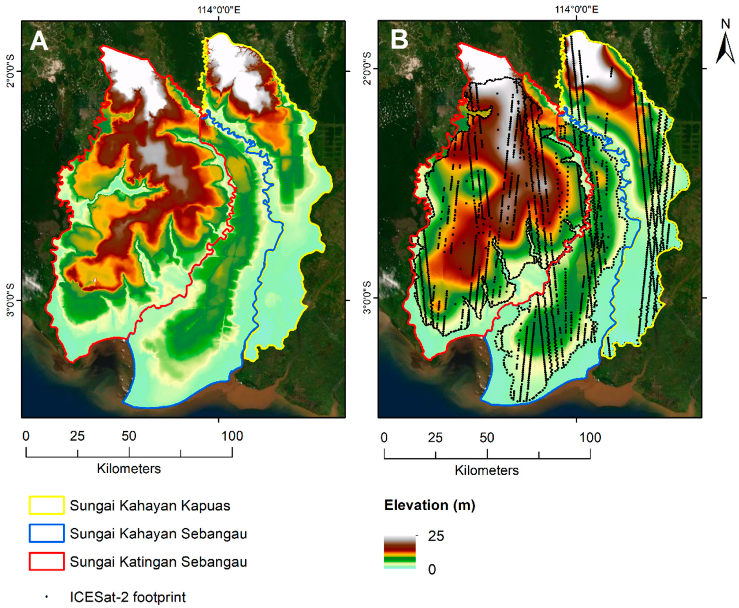
After confirming the ICESat-2 DTM footprints’ accuracy, we investigated if these measurements can be used to model the peat dome surface. This would allow for the detection and mapping of carbon-rich peatlands in areas where no airborne LiDAR or WorldDEM DTM is available. We modeled the surface of three PHUs located on Kalimantan and used the WorldDEM DTM as a reference. The PHU Sungai Katingan Sebangau covers an area of 828,596 ha (red), while PHU Sungai Kahayan Sebangau and Sungai Kahayan Kapuas are smaller, covering 454,542 ha (blue) and 403,013 ha (yellow), respectively (Figure 6). The highest elevations in peat areas are found in the northern part of Sungai Katingan Sebangau and Sungai Kahayan Kapuas, with elevations up to 20 m. In the south, near the coast, the elevation is about 1 m. Sungai Kahayan Sebangau is characterized by lower elevations, ranging from 1 to 9 m. Figure 6 shows that the DTM calculated from interpolated ICESat-2 DTM footprints (Figure 6B) represents the peat surface topography quite well compared to the WorldDEM DTM (Figure 6A. The 12 × 12 m spatial resolution of the WorldDEM DTM shows rivers and larger drainage canals that are not found in the interpolated DTM model, which has a resolution of 100 m. Nevertheless, the convex shape of the peat dome complex is well captured by the interpolated ICESat-2 DTM.
For the validation of the interpolation result, we used random points spread throughout the PHUs. The values per dataset under all random points were extracted and plotted, the result of which is displayed in Table 2. The results show the elevation values of the WorldDEM DTM and interpolated ICESat-2 DTM. The coefficient of determination for Sungai Katingan Sebangau reaches a value of 0.78 using 1300 random points. In the smaller Sungai Kahayan Sebangau, the R2 value is 0.84, based on 700 random points. With an R2 of 0.94 for 950 randomly selected points, the less forested Sungai Kahayan Kapuas produced the strongest correlation. The RMSE is ±2.67 m for Sungai Katingan Sebangau, ±1.47 m for Sungai Kahayan Kapuas, and ±0.68 m for Sungai Kahayan Sebangau. These result in a relative RMSE (coefficient of variation) of 22.5%, 19.09%, and 14.3%, respectively. A visual comparison with optical satellite imagery shows that the highest deviations are in areas with dense forest cover.
The result of the peat dome surface modeling process is shown in Figure 7 for the three PHUs in Sumatra. For these peat dome complexes, airborne LiDAR DTM data were available as a reference for model validation. The ICESat-2 derived DTM model shows that PHU Pulau Padang (Figure 7A, 112.036 ha) consists of a large peat dome with maximal terrain values in the dome’s center. The height reaches about 10 m above the surrounding terrain. The PHU Sungai Mendahara–Sungai Betanghari (Figure 7B, 202.739 ha) is more heterogeneous and consists of two peat domes. PHU Sungai Saleh–Sungai Sugihan (Figure 7C, 191.509 ha) shows a very flat topography; no peat dome is evident. We used 500 random points per PHU for the validation. The comparison of the modeled peat surface with the airborne LiDAR DTM resulted in a coefficient of determination in the range of 0.69 to 0.85 m (Table 3). The RMSE varies from 1.06 to 2.39 m for the different PHUs, with the smallest error in Sungai Mendahara–Sungai Betanghari.
4. Discussion
Mapping the extent and volume of the estimated 20 million ha of tropical peatlands in Indonesia by field-based methods is not feasible because most peatlands are located in remote and highly inaccessible areas. Furthermore, pristine peatlands are covered by very dense and frequently flooded tropical peat swamp forests, which impedes ground surveys most of the year. Even more inaccessible are burned peat swamp forests, which are inaccessible due to broken, partially burned trees and a dense layer of swamp grasses and bushes. To date, only a limited number of field measurements have been collected for selected areas in Sumatra and Kalimantan to assess the extent and volume of carbon-rich ombrogenous peatlands with a dome-shaped surface topography. Information about the peat surface and depth, in combination with drillings, enable the calculation of the peat thickness. Based on the thickness and the known peatland area, the volume and thus the carbon content can be modeled [11,22,25]. The amount of carbon relies on the bulk density (g/cm3) and the carbon content (%), varying for different peat types [11]. Nevertheless, the authors mention uncertainties in the peat volume estimation if the peatlands are located on sloping bedrock. The use of as many drilling measurements as possible enables this limitation to be overcome [7].
Satellite remote sensing can be an efficient tool to map inaccessible peatlands if the dome-shaped surface topography is accessible [7,13]. However, remote sensing sensors must be able to penetrate dense forest cover. The most suitable remote sensing instrument to detect the terrain surface beneath a dense forest canopy is airborne LiDAR [13]. Since airborne data acquisition in remote areas is associated with high costs, it is not a solution to scan large areas. Therefore, a satellite-based system would be the first choice. The SRTM mission recorded the first global topography survey in the year 2000. Since the X-band SAR data of this product do not penetrate the vegetation, especially in dense tropical forests, terrain heights cannot be assessed with sufficient accuracy [7]. A more recent data set is the WorldDEM produced from the TerraSAR-X TanDEM-X radar mission in the years 2012–2014. This high-quality commercial DTM is produced on demand by Airbus. Promising instruments to assess peatland topography are spaceborne LiDAR systems such as ICESat/GLAS and ICESat-2/ATLAS. ICESat/GLAS was successfully applied to map peatland topography by Ballhorn et al. [13] and Hayashi et al. [53].
4.1. The Accuracy of ICESat-2 DTM Footprints
We investigated whether the new spaceborne ICESat-2 LiDAR instrument, with its improved spatial resolution and photon counting system, is suitable to identify and map dome-shaped peatlands based on their specific surface topography. ICESat-2 DTM footprint data quality and accuracy were compared to airborne LiDAR DTM measurements and the radar-based WorldDEM DTM. The LiDAR DTM served as a reference for all comparisons because this data set is considered to be the most accurate within this study (see Section 2.3).
The ICESat-2 DTM showed a vertical accuracy in the range of ±0.34 to 1.09 m compared to the airborne LiDAR DTM. A coefficient of determination of 0.90 showed a strong correlation between the airborne and the ICESat-2 DTM. Within an overlapping area of all three datasets in Kalimantan, the ICESat-2 derived terrain heights in comparison to airborne data (R2 = 0.89) and the WorldDEM DTM data (R2 = 0.86) resulted in strong correlations. Our results are comparable with those of Ballhorn et al. (2011) [13], who analyzed ICESat/GLAS measurements. The ICESat/GLAS DTM data were also compared to airborne LiDAR data and showed a correlation of R2 = 0.91 [13].
We found that in some areas terrain heights were overestimated by ICESat-2. A more detailed investigation showed that this was found in areas covered by dense peat swamp forest, where the spaceborne LiDAR signal did not reach the ground. Neuenschwander et al. [30] identified a decreasing accuracy for ground detection with an increasing density and height of the forest canopy. This is expected since the LiDAR signal has to pass a dense vertical layer of vegetation, and only a few or no photons are reflected from the ground surface. Furthermore, in Neuenschwander and Magruder [54], the authors investigate the potential impact of vertical sampling uncertainty on ICESat-2/ATLAS in different forest ecosystems. The study evaluates simulated ICESat-2 canopy and terrain heights with airborne LiDAR ground-truth data. The results show small mean bias errors and an error uncertainty of 0.06 m (±0.24 m RMSE) and −0.13 m (±0.77 m RMSE) in wooded savannas and boreal forests, respectively. In ecosystems with dense vegetation, terrain errors lay at about 1.93 m (±1.66 m RMSE) and 2.52 m (±2.63 m RMSE). Our analysis in tropical peat swamp forests obtained a similar result with the mean bias error varying from 1.20 to 5.20 m and an RMSE between ±1.88 and 6.13 m. In areas with low-growing vegetation (burned peatland with regrowing vegetation and plantations), we observed a mean bias error of 0.21–0.84 m and an RMSE of ±0.28–0.94 m.
Neuenschwander and Pitts [31] mentioned that ICESat-2/ATLAS can lose its ground signal for canopy closures of >95%, but also when cloud cover obscures the terrestrial signal. Both restrictions are likely in the tropical peat swamp forests of Indonesia. Nevertheless, the forests in the study area often have a canopy closure of less than 95% due to the extreme growth conditions on waterlogged peat. In addition, they are often affected by human activities like logging. In conclusion, it can be stated that peat domes with their smooth topography and convex shape can be clearly identified from space using ICESat-2/ATLAS data. However, the accuracy might be impaired in areas with very dense and tall forests.
4.2. The Accuracy of the Peat Surface Topography Model
We used the discrete ICESat-2 DTM measurements to create a spatially inclusive and comprehensive model of the surface topography of various large peat dome complexes in Kalimantan and Sumatra. The modeled surface of the six peatlands based on ICESat-2 measurements, using ordinary kriging, correlates well with the WorldDEM DTM data in Kalimantan (R2 = 0.78, 0.84, and 0.94) and airborne LiDAR DTM data in Sumatra (R2 = 0.69, 0.72, and 0.85). In addition, the interpolated terrain shows a similar value distribution as the reference DTMs. However, small-scale features like small rivers or drainage canals are not well represented by the current model, because the number of ICESat-2 DTM measurements is currently still too low. This will improve in the future when more orbits are recorded. Recalculation of the model with an increasing number of DTM footprints will improve the spatial detail of the peat surface topography model.
4.3. Potential Error Sources
Differences in resolution and extent also mean that different ground areas influence the derived pixel value [55]. For an accurate comparison of the three datasets: airborne LiDAR, WorldDEM, and ICESat-2, we overcame the problem of different resolutions by using the mean of all pixels per dataset. However, there may still be negligible deviations because of edge effects. Furthermore, different sensor accuracies have to be considered. The airborne LiDAR DTM has a field validated vertical accuracy of 0.18 m [35]. ICESat-2 has a ranging precision of 25–35 cm in flat terrain [30,31]. In steeper terrain, the sloping topography is incorporated as a function of the “geolocation knowledge of the pointing multiplied by the tangent of the surface slope” [31]. Since the study area is in a flat region of coastal areas in Indonesia, we assume a ranging precision no higher than 35 cm on bare ground. The global model of the WorldDEM DTM has a relative vertical accuracy of <5 m, while for flat terrain, as for the study area, the vertical accuracy in comparison with the airborne DTM lies at ±0.47 m. Regarding the size of the investigated area, individual sensor inaccuracies are negligibly small [7].
In addition to the different spatial resolutions, acquisition geometries, and sensor accuracies, the different acquisition times of the sensors can lead to potential errors. During the acquisitions, peat loss due to peat decomposition in drained areas can result in subsidence. The subsidence rate for peatlands in Sumatra and Kalimantan ranges from 2 to 4 cm/year, depending on the distance to draining canals and the unaffected forest cover of the respective peatland [56]. This is less than the accuracy of any of the DTM data sets, which we used in this study. Furthermore, note that the transformation to normal distribution and the back-transformation can introduce a bias [57,58,59].
5. Conclusions
We showed that carbon-rich ombrogenous peatlands can be identified based on terrain heights derived from ICESat-2 DTM footprint data. Furthermore, we demonstrated that it is possible to interpolate a seamless surface model from the ICESat-2 orbit track footprints in Indonesia using ordinary kriging. Knowing the surface topography, in combination with the peat dome depth, allows estimating the peat’s volume. Based on the volume, carbon content, and bulk density, the potential carbon store of the peat dome can be calculated.
The surface interpolation based on ICESat-2 DTM footprints was applied and validated in different peatlands in Sumatra and Kalimantan, and proved to be fast and robust. Since ICESat-2 data are distributed for free, this data source is a cost-efficient alternative to the more expensive commercial data sets, such as airborne LiDAR or the WorldDEM DTM. By 2022, ICESat-2 will reach almost global coverage, providing flight lines with a distance of less than 2 km at the equator. These dense measurements will further enhance the surface interpolation model of peatlands and can contribute to the estimation of the carbon storage of this ecosystem.
Besides accurate terrain height measurements, the canopy height provided by ICESat-2 showed great potential for gaining information about tropical forests, such as the canopy height, which can enable the modeling of aboveground biomass—another essential parameter for deriving the carbon content. Highly accurate estimations of both aboveground and belowground carbon contents are significant input variables for global climate models and thus provide a crucial contribution to emission reduction projects.
The new mission Global Ecosystem Dynamics Investigation (GEDI), a high-powered laser system operating from the ISS, provides additional information between 52° north and south. The distance of GEDI’s flight tracks is approximately 600 m, which further improves the global coverage of publicly accessible LiDAR data. A combination of ICESat-2 and GEDI data will offer the possibility to further improve the surface interpolation. Furthermore, the satellite-based canopy height measurements might contribute to the aboveground biomass estimation in vast, remote, and inaccessible peatland ecosystems.
Author Contributions
A.B. and F.S. conceived and designed the experiments; A.B. collected, prepared, and analyzed the data; A.B. wrote the manuscript; and F.S. reviewed and commented on the manuscript. All authors have read and agreed to the published version of the manuscript.
Funding
This research received no external funding.
Conflicts of Interest
The authors declare no conflict of interest.
References
- Murdiyarso, D.; Saragi-Sasmito, M.F.; Rustini, A. Greenhouse gas emissions in restored secondary tropical peat swamp forests. Mitig. Adapt. Strateg. Glob. Chang. 2019, 24, 507–520. [Google Scholar] [CrossRef]
- Posa, M.R.C.; Wijedasa, L.S.; Corlett, R.T. Biodiversity and conservation of tropical peat swamp forests. BioScience 2011, 61, 49–57. [Google Scholar] [CrossRef]
- Estoque, R.C.; Ooba, M.; Avitabile, V.; Hijioka, Y.; DasGupta, R.; Togawa, T.; Murayama, Y. The future of Southeast Asia’s forests. Nat. Commun. 2019, 10, 1829. [Google Scholar] [CrossRef] [PubMed] [Green Version]
- Izquierdo, N.L. Formation of Tropical Peatlands. Available online: https://www.grida.no/resources/12531 (accessed on 4 June 2020).
- Page, S.E.; Rieley, J.O.; Wüst, R. Lowland tropical peatlands of Southeast Asia. Peatl. Evol. Rec. Environ. Clim. Chang. 2006, 9, 145–172. [Google Scholar] [CrossRef]
- Page, S.E.; Banks, C.J.; Rieley, J.O. Tropical peatlands: Distribution, extent and carbon storage–Uncertainties and knowledge gaps. Peatl. Int. 2007, 2, 1–7. [Google Scholar]
- Jaenicke, J.; Rieley, J.O.; Mott, C.; Kimman, P.; Siegert, F. Determination of the amount of carbon stored in Indonesian peatlands. Geoderma 2008, 147, 151–158. [Google Scholar] [CrossRef]
- Page, S.E.; Rieley, J.O.; Banks, C.J. Global and regional importance of the tropical peatland carbon pool. Glob. Chang. Biol. 2011, 17, 798–818. [Google Scholar] [CrossRef] [Green Version]
- Warren, M.; Hergoualc’h, K.; Kauffman, J.B.; Murdiyarso, D.; Kolka, R. An appraisal of Indonesia’s immense peat carbon stock using national peatland maps: Uncertainties and potential losses from conversion. Carbon Balance Manag. 2017, 12, 12. [Google Scholar] [CrossRef]
- Page, S.E.; Wűst, R.A.J.; Weiss, D.; Rieley, J.O.; Shotyk, W.; Limin, S.H. A record of Late Pleistocene and Holocene carbon accumulation and climate change from an equatorial peat bog (Kalimantan, Indonesia): Implications for past, present and future carbon dynamics. J. Quat. Sci. 2004, 19, 625–635. [Google Scholar] [CrossRef]
- Agus, F.; Hairiah, K.; Mulyani, A. Measuring Carbon Stock in Peat Soils. Practical Guidelines; World agroforestry centre (ICRAF) Southeast Asia regional program; Indonesian Centre for Agricultural Land Resources Research and Development: Bogor Jawa Barat, Indonesia, 2011; ISBN 9789793198668. [Google Scholar]
- Page, S.E.; Hooijer, A. In the line of fire: The peatlands of Southeast Asia. Philos. Trans. R. Soc. Lond. B. Biol. Sci. 2016, 371. [Google Scholar] [CrossRef] [Green Version]
- Ballhorn, U.; Jubanski, J.; Siegert, F. ICESat/GLAS data as a measurement tool for peatland topography and peat swamp forest biomass in Kalimantan, Indonesia. Remote Sens. 2011, 3, 1957–1982. [Google Scholar] [CrossRef] [Green Version]
- Dinsmore, K.J.; Skiba, U.M.; Billett, M.F.; Rees, R.M. Effect of water table on greenhouse gas emissions from peatland mesocosms. Plant Soil 2009, 318, 229–242. [Google Scholar] [CrossRef] [Green Version]
- Carlson, K.M.; Goodman, L.K.; Calen, C.M.T. Modeling relationships between water table depth and peat soil carbon loss in Southeast Asian plantations. Environ. Res. Lett. 2015, 10, 74006. [Google Scholar] [CrossRef]
- Wetlands International. Peatland Distribution in Sumatra and Kalimantan: Explanation of Its Data Sets Including Source of Information, Data Constraints and Gaps, Bogor. 2008. Available online: https://indonesia.wetlands.org/publications/peatland-distribution-in-sumatra-and-kalimantan-explanation-of-its-data-sets-including-source-of-information-accuracy-data-constraints-and-gap/ (accessed on 29 March 2020).
- Ballhorn, U. Airborne and Spaceborne LiDAR Data as a Measurement Tool for Peatland Topography, Peat Fires Burn Depth, and Forest Above Ground Biomass in Central Kalimantan, Indonesia. Ph.D. Dissertation, Ludwig-Maximilian-University, Munich, Germany, 2012. [Google Scholar]
- Bourdeau, J.; Nelson, R.F.; Margolis, H.A.; Beaudion, A.; Guidon, L.; Kimes, D. Regional aboveground forest biomass using airborne and spaceborne LiDAR in Québec. Remote Sens. Environ. 2008, 112, 3876–3890. [Google Scholar] [CrossRef]
- Carabajal, C.C.; Harding, D. SRTM C-band and ICESat laser altimetry elevation comparisons as a function of tree cover and relief. Photogramm. Eng. Remote Sens. 2006, 72, 287–298. [Google Scholar] [CrossRef] [Green Version]
- Harding, D.J.; Carabajal, C.C. ICESat waveform measurements of within-footprint topographic relief and vegetation vertical structure. Geophys. Res. Lett. 2005, 32, 2509. [Google Scholar] [CrossRef] [Green Version]
- Liu, M.; Popescu, S.; Malambo, L. Feasibility of burned area mapping based on ICESAT−2 photon counting data. Remote Sens. 2020, 12, 24. [Google Scholar] [CrossRef] [Green Version]
- Jaenicke, J.; Wösten, H.; Budiman, A.; Siegert, F. Planning hydrological restoration of peatlands in Indonesia to mitigate carbon dioxide emissions. Mitig. Adapt. Strateg. Glob. Chang. 2010, 15, 223–239. [Google Scholar] [CrossRef] [Green Version]
- Silvestri, S.; Knight, R.; Viezzoli, A.; Richardson, C.J.; Anshari, G.Z.; Dewar, N.; Flanagan, N.; Comas, X. Quantification of peat thickness and stored carbon at the landscape scale in tropical peatlands: A comparison of airborne geophysics and an empirical topographic method. J. Geophys. Res. Earth Surf. 2019, 124, 3107–3123. [Google Scholar] [CrossRef] [Green Version]
- Dommain, R.; Couwenberg, J.; Joosten, H. Hydrological self-regulation ofdomed peat swamps in south-east Asia and consequences for conservation andrestoration. Mires Peat 2010, 6, 1–17. [Google Scholar]
- Nasrul, B.; Maas, A.; Utami, S.N.H.; Nurudin, M. The relationship between surface topography and peat thickness on Tebing Tinggi Island, Indonesia. Mires. Peat. 2020, 26, 1–21. [Google Scholar] [CrossRef]
- Englhart, S.; Jubanski, J.; Siegert, F. Quantifying dynamics in tropical peat swamp forest biomass with multi-temporal LiDAR datasets. Remote Sens. 2013, 5, 2368–2388. [Google Scholar] [CrossRef] [Green Version]
- Matheron, G. The Theory of Regionalized Variables and Its Applications; École Nationale Supérieure des Mines: Paris, France, 1971. [Google Scholar]
- Siegert, F.; Ruecker, G.; Hinrichs, A.; Hoffmann, A.A. Increased damage from fires in logged forests during droughts caused by El Niño. Nature 2001, 437–440. [Google Scholar] [CrossRef] [PubMed]
- Ballhorn, U.; Siegert, F.; Mason, M.; Limin, S. Derivation of burn scar depths and estimation of carbon emissions with LIDAR in Indonesian peatlands. Proc. Natl. Acad. Sci. USA 2009, 106, 21213–21218. [Google Scholar] [CrossRef] [Green Version]
- Neuenschwander, A.; Pitts, K. The ATL08 land and vegetation product for the ICESat-2 Mission. Remote Sens. Environ. 2019, 221, 247–259. [Google Scholar] [CrossRef]
- Neuenschwander, A.; Pitts, K. Ice, Cloud, and Land Elevation Satellite 2 (ICESat-2) Algorithm Theoretical Basis Document (ATBD) for Land–Vegetation Along-Track Products (ATL08); National Aeronautics and Space Administration (NASA), 2019. Available online: https://icesat-2.gsfc.nasa.gov/sites/default/files/files/ATL08_15June2018.pdf (accessed on 12 April 2020).
- Pavlis, N.K.; Holmes, S.A.; Kenyon, S.C.; Factor, J.K. The development and evaluation of the Earth gravitational model 2008 (EGM2008). J. Geophys. Res. 2012, 117. [Google Scholar] [CrossRef] [Green Version]
- Geographic Lib. Geoid Height. Available online: https://geographiclib.sourceforge.io/html/geoid.html#geoidinst (accessed on 18 April 2020).
- Ballhorn, U.; Navratil, P.; Jubanski, J.; Siegert, F. LiDAR Survey of the Kalimantan Forests and Climate Partnership (KFCP) Project Site and EMRP Area in Central Kalimantan; Technical Working Paper; Remote Sensing Solutions GmbH: Munich, Germany, 2014. [Google Scholar]
- Konecny, K.; Ballhorn, U.; Navratil, P.; Jubanski, J.; Page, S.E.; Tansey, K.; Hooijer, A.; Vernimmen, R.; Siegert, F. Variable carbon losses from recurrent fires in drained tropical peatlands. Glob. Chang. Biol. 2016, 22, 1469–1480. [Google Scholar] [CrossRef] [Green Version]
- Suppa, M. WorldDEM™ Technical Product Specification. Digital Surface Model, Digital Terrain Model Version 2.0; Airbus Defence and Space Intelligence, 2015; Available online: https://www.intelligence-airbusds.com/files/pmedia/public/r51492_9_2019-04_worlddem_technicalspecs_version2.5_i1.0.pdf (accessed on 29 March 2020).
- Markus, T.; Neumann, T.; Martino, A.; Abdalati, W.; Brunt, K.; Csatho, B.; Farrell, S.; Fricker, H.; Gardner, A.; Harding, D.; et al. The ice, cloud, and land elevation satellite-2 (ICESat-2): Science requirements, concept, and implementation. Remote Sens. Environ. 2017, 190, 260–273. [Google Scholar] [CrossRef]
- Neuenschwander, A.L.; Magruder, L.A. Canopy and terrain height retrievals with ICESat-2: A first look. Remote Sens. 2019, 11, 1721. [Google Scholar] [CrossRef] [Green Version]
- Barton, J.M.H.; Buchberger, S.G.; Lange, M.L. Estimation of error and compliance in surveys by kriging. J. Surv. Eng. 1999, 125, 87–108. [Google Scholar] [CrossRef]
- Jassim, F.A.; Altaany, F. Image interpolation using kriging technique for spatial data. Can. J. Image Process. Comp. Vis. 2013, 4, 16–21. [Google Scholar]
- Yilmaz, M.; Uysal, M. Comparing uniform and random data reduction methods for DTM accuracy. Int. J. Eng. Geosci. 2017, 2, 9–16. [Google Scholar] [CrossRef] [Green Version]
- Ferreira, I.O.; Rodrigues, D.D.; Santos, G.R.D.; Ferraz Rosa, L.M. In bathymetric surfaces: IDW or kriging? Bol. Ciênc. Geod. 2017, 23, 493–508. [Google Scholar] [CrossRef] [Green Version]
- Wojciech, M. Kriging method optimization for the process of DTM creation based on huge data sets obtained from MBESs. Geosciences 2018, 8, 433. [Google Scholar] [CrossRef] [Green Version]
- Oliver, M.A.; Webster, R. Kriging: A method of interpolation for geographical information systems. Int. J. Geograph. Inf. Syst. 1990, 4, 313–332. [Google Scholar] [CrossRef]
- Webster, R.; Oliver, M.A. Geostatistics for Environmental Scientists, 2nd ed.; John Wiley & Sons Ltd.: Chichester, UK, 2007. [Google Scholar]
- Handbook of spatial analysis. In Theory and Practical Application with R; Loonis, V.; Bellefon, M.P. (Eds.) Montrouge Cedex, Institut National de la Statistique et des Études Économiques (INSEE): Montrouge, France, 2018. [Google Scholar]
- Hengl, T. A Practical Guide to Geostatistical Mapping, 2nd ed.; Hengl: Amsterdam, The Netherlands, 2009; ISBN 9090249818. [Google Scholar]
- Peterson, R.A.; Cavanaugh, J.E. Ordered quantile normalization: A semiparametric transformation built for the cross-validation era. J. Appl. Stat. 2019, 47, 2312–2327. [Google Scholar] [CrossRef]
- Sakizadeh, M.; Mohamed, M.A.M.; Klammler, H. Trend analysis and spatial prediction of groundwater levels using time series forecasting and a novel spatio-temporal method. Water Resour. Manag. 2019, 33, 1425–1437. [Google Scholar] [CrossRef]
- Bhowmik, A.K.; Cabral, P. Spatially shifting temporal points: Estimating pooled within-time series variograms for scarce hydrological data. Hydrol. Earth Syst. Sci. Discuss. 2015, 12, 2243–2265. [Google Scholar] [CrossRef] [Green Version]
- Weller, Z.D.; Hoeting, J.A. A Review of Nonparametric Hypothesis Tests of Isotropy Properties in Spatial Data. Statistical Science 2016. Available online: http://arxiv.org/pdf/1508.05973v2 (accessed on 9 December 2020).
- Pebesma, E.J. Gstat User’s Manual; Department of Physical Geography, Utrecht University: Utrecht, The Netherlands, 2014. [Google Scholar]
- Hayashi, M.; Saigusa, N.; Yamagata, Y.; Hirano, T. Regional forest biomass estimation using ICESat/GLAS spaceborne LiDAR over Borneo. Carbon Manag. 2015, 6, 19–33. [Google Scholar] [CrossRef]
- Neuenschwander, A.; Magruder, L. The potential impact of vertical sampling uncertainty on ICESat-2/ATLAS terrain and canopy height retrievals for multiple ecosystems. Remote Sens. 2016, 8, 1039. [Google Scholar] [CrossRef] [Green Version]
- Frazer, G.W.; Magnussen, S.; Wulder, M.A.; Niemann, K.O. Simulated impact of sample plot size and co-registration error on the accuracy and uncertainty of LiDAR-derived estimates of forest stand biomass. Remote Sens. Environ. 2011, 115, 636–649. [Google Scholar] [CrossRef]
- Vernimmen, R.; Hooijer, A.; Akmalia, R.; Fitranatanegara, N.; Mulyadi, D.; Yuherdha, A.; Andreas, H.; Page, S. Mapping deep peat carbon stock from a LiDAR based DTM and field measurements, with application to eastern Sumatra. Carbon Balance Manag. 2020, 15, 4. [Google Scholar] [CrossRef] [PubMed]
- Wilson, B.G.; Adam, B.J.; Karney, B.W. Bias in log-transformed frequency distributions. J. Hydrol. 1990, 118, 19–37. [Google Scholar] [CrossRef]
- Newman, M.C. Regression analysis of log-transformed data: Statistical bias and its correction. Environ. Toxicol. Chem. 1993, 12, 1129–1133. [Google Scholar] [CrossRef]
- Yamamoto, J.K. On unbiased back-transform of lognormal kriging estimates. Comput. Geosci. 2007, 11, 219–234. [Google Scholar] [CrossRef]
Figure 1.
Schematic overview of the formation of peat domes in Indonesia and other tropical countries. Dead plant material accumulates in a water-filled depression that lacks oxygen. The accumulation rate is about 0.5–2 mm per year. After thousands of years, a convex-shaped peat dome up to a several meters thick is formed. The dome is generally covered by forests such as peat swamp forest (figure is taken from [4]).

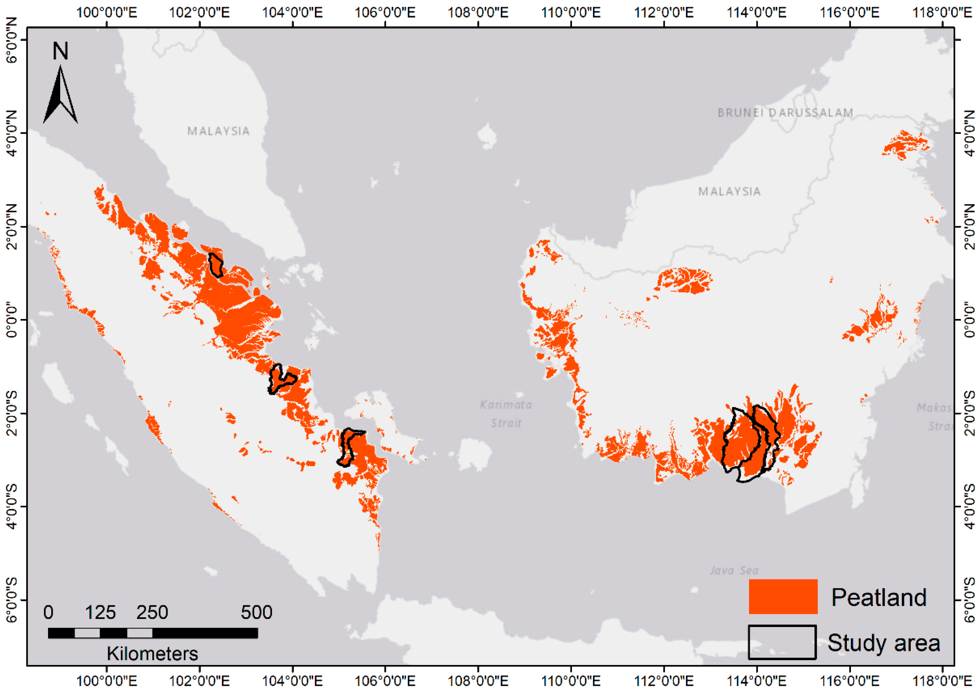
Figure 2.
Overview of the known peatlands in Kalimantan and Sumatra, Indonesia (brown). In total, the Indonesian peatlands cover an area of approximately 200,000 km2. Black outlines indicate the six hydrological units that were investigated, which cover more than 10% (21.924 km2) of the peatland area in Indonesia. Sungai Katingan Sebangau, Sungai Kahayan Sebangau, and Sungai Kahayan Kapuas (from west to east) are in Central Kalimantan, and Pulau Padang (north), Sungai Mendahara–Sungai Betanghari (center), and Sungai Saleh–Sungai Sugihan (south) are located on Sumatra.

Figure 3.
Scatterplot demonstrating the correlation between airborne and ICESat-2 derived DTM measurements. Right panel: the map displays an airborne LiDAR DTM of a large peat hydrological unit (PHU) peatland complex (Sungai Kahayan Sebangau and Sungai Kahayan Kapuas in Central Kalimantan, north–south extent >100 km). Raised peat domes are visible in dark green to dark brown to white colors. Superimposed are the ICEatS-2 footprints shown as red dots. The black line indicates the location of the transect shown in Figure 4.

Figure 4.
The disturbance of the ICESat-2 DTM by different land covers as detected along a 42 km north–south transect. The transect covers dense and tall peat swamp forests, previously burned forests, and a recently planted oil palm plantation. (A) Airborne LiDAR DTM—the peat dome descends from north to south by approximately 8 m. Green colors indicate low-lying terrain while brown indicates higher elevations. (B) Sentinel-2 satellite image acquired in October 2019 (bands SWIR, NIR, Red) showing forest areas in green, burned areas in pink, and oil palms in bright green. (B1–B3) Enlarged areas indicated by black rectangles in B. (B1) Tall peat swamp forest. (B2) Burned forest with regrown shrubs and trees. (B3) Plantation. (C) Height profile of the airborne DTM (gray) and the ICESat-2 DTM measurements (red dots). Green dots show the canopy height as measured by ICESat-2. Bounding boxes B1, B2, and B3 represent the height profiles of the specific areas within B.

Figure 5.
Comparison of the airborne DTM and ICESat-2 DTM along an 88 km-long transect (red line) across four large peat domes. The four peat domes are clearly visible by their convex curvature. (A) The airborne DTM covers an elevation range of 3 to 12 m displayed in green to brown colors. (B) Height profile of the transect from west to east. The gray line represents the airborne LiDAR DTM and the red dots show the corresponding ICESat-2 DTM.

Figure 6.
Comparison of the DTM of three PHU. A shows the WorldDEM DTM; the B shows the peat dome surface model obtained by interpolating all available ICESat-2 footprint DTM measurements. ICESat-2 footprints used for the interpolation are shown as black circles.
Figure 6.
Comparison of the DTM of three PHU. A shows the WorldDEM DTM; the B shows the peat dome surface model obtained by interpolating all available ICESat-2 footprint DTM measurements. ICESat-2 footprints used for the interpolation are shown as black circles.

Figure 7.
Peat surface modeling results for three large PHU in Sumatra. Pulau Padang (A), Sungai Mendahara–Sungai Betanghari (B) and Sungai Saleh–Sungai Sugihan (C). ICESat-2 footprints used for the interpolation are shown as black circles.
Figure 7.
Peat surface modeling results for three large PHU in Sumatra. Pulau Padang (A), Sungai Mendahara–Sungai Betanghari (B) and Sungai Saleh–Sungai Sugihan (C). ICESat-2 footprints used for the interpolation are shown as black circles.


Table 1.
Comparison of measured elevation from different tested sensors (Npoints = 13.129).
| Sensor Comparison | Mean Elevation (m) | R2 | RMSE (m) |
|---|---|---|---|
| Airborne – WorldDEM DTM | 3.35 3.30 | 0.95 | ±0.47 |
| Airborne – ICESat-2 | 3.35 3.69 | 0.89 | ±0.83 |
| WorldDEM DTM – ICESat-2 | 3.30 3.69 | 0.94 | ±0.86 |
Table 2.
Comparison of the DTM based on airborne data and ordinary kriging (OK) results for the different PHUs located on Sumatra (Sungai Katingan Sebangau, Npoints = 1300; Sungai Kahayan Sebangau, Npoints = 700; Sungai Kahayan Kapuas, Npoints = 950).
Table 2.
Comparison of the DTM based on airborne data and ordinary kriging (OK) results for the different PHUs located on Sumatra (Sungai Katingan Sebangau, Npoints = 1300; Sungai Kahayan Sebangau, Npoints = 700; Sungai Kahayan Kapuas, Npoints = 950).
| PHU | Sensor | Mean Elevation (m) | R2 | RMSE (m) |
|---|---|---|---|---|
| Sungai Katingan Sebangau | WorldDEM OK model | 11.86 12.50 | 0.78 | ±2.67 |
| Sungai Kahayan Sebangau | WorldDEM OK model | 4.57 4.33 | 0.84 | ±0.68 |
| Sungai Kahayan Kapuas | WorldDEM OK model | 7.70 7.27 | 0.97 | ±1.47 |
Table 3.
Comparison of the elevation based on airborne data and ordinary kriging (OK) results for the different PHUs located on Sumatra (Npoints = 500 per PHU).
Table 3.
Comparison of the elevation based on airborne data and ordinary kriging (OK) results for the different PHUs located on Sumatra (Npoints = 500 per PHU).
| PHU | Sensor | Mean Elevation (m) | R2 | RMSE (m) |
|---|---|---|---|---|
| Pulau Padang | Airborne OK model | 5.81 7.65 | 0.72 | ±2.39 |
| Sungai Mendahara–Sungai Betanghari | Airborne OK model | 3.82 4.36 | 0.85 | ±1.06 |
| Sungai Saleh–Sungai Sugihan | Airborne OK model | 2.72 3.14 | 0.69 | ±1.13 |
Publisher’s Note: MDPI stays neutral with regard to jurisdictional claims in published maps and institutional affiliations. |
© 2020 by the authors. Licensee MDPI, Basel, Switzerland. This article is an open access article distributed under the terms and conditions of the Creative Commons Attribution (CC BY) license (http://creativecommons.org/licenses/by/4.0/).
Share and Cite
MDPI and ACS Style
Berninger, A.; Siegert, F. The Potential of ICESat-2 to Identify Carbon-Rich Peatlands in Indonesia. Remote Sens. 2020, 12, 4175. https://0-doi-org.brum.beds.ac.uk/10.3390/rs12244175
AMA Style
Berninger A, Siegert F. The Potential of ICESat-2 to Identify Carbon-Rich Peatlands in Indonesia. Remote Sensing. 2020; 12(24):4175. https://0-doi-org.brum.beds.ac.uk/10.3390/rs12244175
Chicago/Turabian StyleBerninger, Anna, and Florian Siegert. 2020. "The Potential of ICESat-2 to Identify Carbon-Rich Peatlands in Indonesia" Remote Sensing 12, no. 24: 4175. https://0-doi-org.brum.beds.ac.uk/10.3390/rs12244175
Note that from the first issue of 2016, this journal uses article numbers instead of page numbers. See further details here.