Article

Spatiotemporal Analysis of Hydrological Variations and Their Impacts on Vegetation in Semiarid Areas from Multiple Satellite Data

1
College of Civil Engineering and Architecture, Yan’an University, Yan’an 716000, China
2
Key Laboratory of Subsurface Hydrology and Ecological Effects in Arid Region, Ministry of Education, Chang’an University, Xi’an 710054, China
3
School of Water and Environment, Chang’an University, Xi’an 710054, China
4
Water Conservancy and Civil Engineering College, Inner Mongolia Agricultural University, Hohhot 001018, China
*
Author to whom correspondence should be addressed.
Remote Sens. 2020, 12(24), 4177; https://0-doi-org.brum.beds.ac.uk/10.3390/rs12244177
Submission received: 7 November 2020 / Revised: 9 December 2020 / Accepted: 16 December 2020 / Published: 20 December 2020
(This article belongs to the Special Issue Remote Sensing in Hydrology and Water Resources Management)

Abstract

:
Understanding the spatiotemporal characteristics of hydrological components and their impacts on vegetation are critical for comprehending hydrological, climatological, and ecological processes under environmental change and solving future water management challenges. Innovative methods need to be developed in semiarid areas to analyze the special hydrological factors in the water resource systems of these areas. Gravity Recovery and Climate Experiment (GRACE) and Global Land Data Assimilation System (GLDAS) were applied with the normalized difference vegetation index (NDVI) data in this paper to analyze spatiotemporal changes of hydrological factors in the Xiliaohe River Basin (XRB). The results showed that precipitation (P), evapotranspiration (ET) and temperature (T) had similar seasonal change patterns at rates of 0.05 cm/yr., 0.01 cm/yr. and −0.05 °C/yr., respectively. Total water storage change (TWSC) was consistent with the change trend of soil moisture change (SMC) and showed a fluctuating trend. Groundwater change (GWC) showed a decreasing trend at a rate of −0.43 cm/yr. P and ET had a greater impact on GLDAS data (R = 0.634, P < 0.05 and R = 0.686, P < 0.01, respectively) than on other factors. GWC was more sensitive to changes in T (R = 0.570, P < 0.05). Furthermore, a lag period of 0 to 1 months was observed for the effects of P and ET on TWSC and GLDAS. NDVI showed an upward trend at a rate of 0.001 yr−1 between 2002 and 2014. A spatial distribution of NDVI was heterogeneous in the study area. ET, GLDAS and GWC in growing season limited vegetation growth and were more important than other factors in XRB. The results may contribute to an understanding of the relationships between the hydrological cycle and climate change and provide scientific support for local environmental management.

Graphical Abstract

1. Introduction

Approximately 30% of continental land area is characterized as arid and semiarid [1]. Water cycle conditions and vegetation ecosystems are fragile and sensitive in these areas [2], and increasing water demand from all kinds of water users has seriously impacted vegetation ecosystems. Along with climate change, this increase in demand has greatly changed hydrological factors and water balance in semiarid areas [3,4]. The Xiliaohe River Basin (XRB) has experienced dramatic changes in its hydrological cycle and water balance [5,6,7]. Distribution and growth of vegetation have changed observably in the area, which may be related to the important role of hydrological factors in a vegetation ecological environment [8,9]. It is within this context that hydrological changes and their impact on vegetation are among the key issues in semiarid areas, where water resources are scarce and the ecological environment is fragile.
XRB is an agropastoral ecotone in a semiarid area that has experienced significant climate change [10], with an average annual temperature (T) increase of 0.5–0.7 °C. At the same time, the groundwater level in the study area decreased notably from 2 m to 6 m over the past 30 years due to unrestrained development and water resource use [11]. Water cycle at the regional scale has been directly affected by regional climate change and groundwater overexploitation, which had impacts in local vegetation change and distribution [12]. Precipitation (P) at 46 meteorological stations decreased from 1960–2012 in Inner Mongolia [13], and P in XRB showed a similar decreasing trend, which led to decreased discharge from the four inbound rivers and a significant decrease in the groundwater level from 1951 to 2007 [14]. Meanwhile, evapotranspiration (ET) (determined by the Penman-Monteith method) varied significantly in both time and space in the area [15,16]. Relationships between hydrological factors were analyzed based on the results at a few observation points [17,18] and thus could not well represent the spatial heterogeneity because of the limited observation points. Some conventional hydrological and climatic indicators have also been used to analyze the hydrological variations and their impacts on the vegetation [13,19]. However, these results could not reveal the balance of regional water resources and its impact on vegetation change, especially on a different scale. Moreover, due to the limited number of observations at the regional scale and in remote areas, data on certain hydrological and meteorological factors may not be available, such as the change in the total water storage change (TWSC), soil moisture change (SMC), groundwater storage change (GWC), etc. Thus, determining the hydrological, climatological and ecological processes may be difficult. Now, this is possible using satellite techniques for monitoring land meteorological and hydrological characteristics [11,20]. Since Gravity Recovery and Climate Experiment (GRACE) satellite launch in March 2002, it has provided a unique way to monitor changes in the earth’s gravitational field, especially terrestrial water reserve changes at a regional scale [21]. At present, many achievements have been harvested in related fields, such as hydrological characteristics of TWSC, which were estimated in many regional basins, e.g., China [22], Tarim River basin [23] and so on. Moreover, GWC could also be detected on different spatial scales [24,25]. Zhong et al. [11] found that the GWS showed a prolonged declining rate of −17.8 ± 0.1 mm/yr. during 1971–2015 in the North China Plain, based on in situ groundwater-level measurements and satellite observations. Han et al. [26] discussed the GWC dynamic at multi-timescales in Yunnan Province and the correlations with extreme meteorological factors. Lv et al. [27] found that human factors were the main influencing factors of regional hydrological characteristics, through analyzing the quantitative attribution of terrestrial water storage (TWS) variation from hydroclimatic and anthropogenic factors. In addition, the accuracy of GWC retrieved from the GRACE satellite data in a semiarid area was verified by a comparison with in-situ data [11]. In these analyses, regional hydrological characteristics dynamics and their correlation with meteorological factors are analyzed, thus ignoring the lag time between them. In contrast, more attention to the correlations between regional hydrological characteristics and meteorological factors at multiple-time scales were paid in this paper. Furthermore, in order to fully reveal the impacts of hydrological variations on vegetation in semiarid areas, their evolution characteristics at multiple-time scales and spatial scale were examined.
In summary, spatiotemporal changes of hydrological and meteorological factors, such as P, ET, T, TWSC, SMC and GWC, etc., especially their impacts on vegetation in XRB, have rarely been comprehensively discussed. This paper analyzed regional water balance and vegetation factors based on data from multiple satellite observations. Comprehensive correlations among climatological, hydrological, and vegetation factors in XRB were simultaneously analyzed using time-series data from 2002 to 2014 at the regional scale. The main objectives of this study are (1) to analyze spatiotemporal dynamic of hydrological factors and normalized difference vegetation index (NDVI) in agropastoral ecotone of semiarid region based on multiple satellite data, (2) analyze response relationships among regional hydrometeorological factors at multiple-time scales, and (3) evaluate the impacts of hydrological variations on vegetation.

2. Materials and Methods
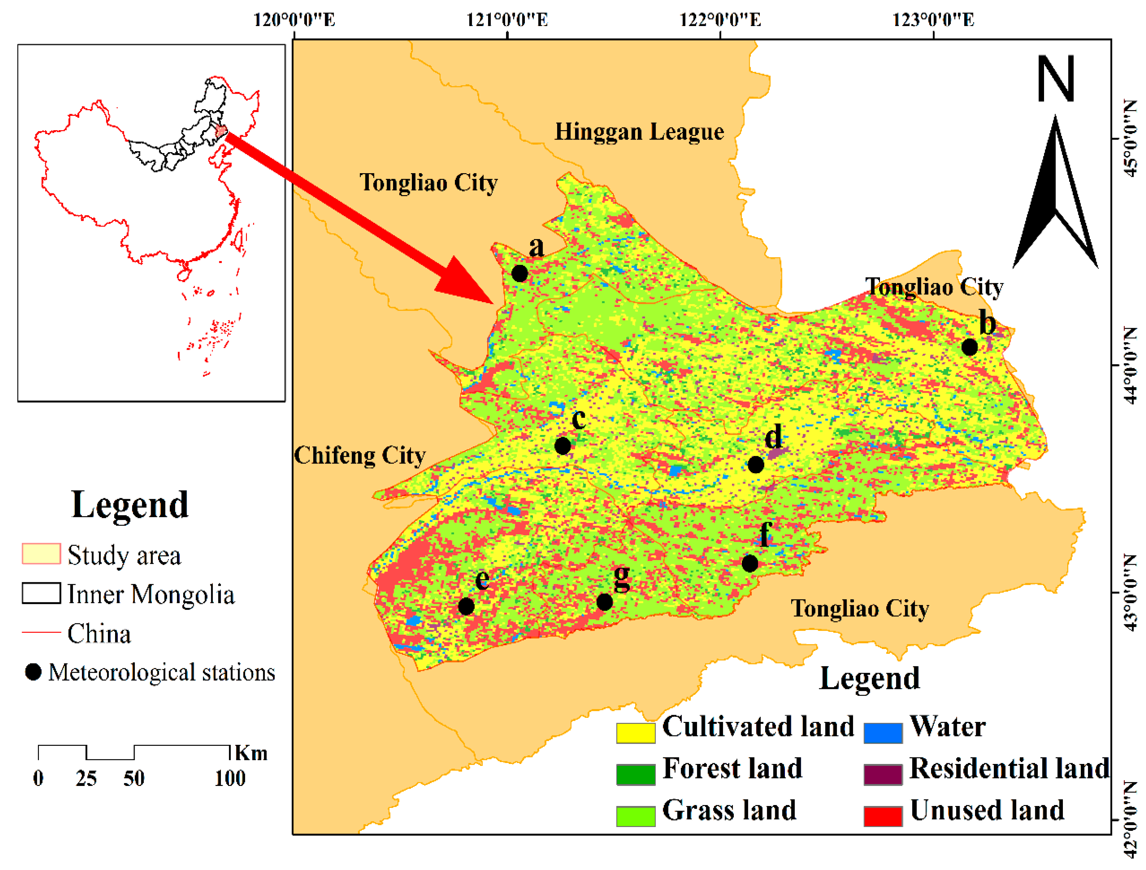
2.1. Study Area

Xiliaohe River Basin (XRB), Inner Mongolia Autonomous Region, northeast part of China, lies between the latitude 42°30′ to 45°00′ N and longitude 120°00′ to 123°30′ E (Figure 1), which has an area of 3.2 × 10⁴ km2 and an average elevation of 800 m (400~1300 m). Three main rivers once flowed through the study area: Xiliao River, Jiaolai River, and Xinkai River. However, the rivers’ discharge has been reduced and may even dry up either seasonally or perennially [28]. Moreover, the increased water demand from irrigation in recent decades has led groundwater to become the main total terrestrial water storage source supplied to meet agricultural, industrial, and domestic water demand. The overexploitation and utilization of groundwater has caused various environmental problems [29], e.g., regional groundwater table and pollution, land subsidence, and ecological environment deterioration.
In XRB, annual precipitation ranged from 350 mm to 450 mm, the annual average temperature was 6.0°C, and the pan evaporation (Φ 20 cm) was 1817 mm [30]. Approximately 80% of the total precipitation occurs in summer (June to September). As a typical ecotone between Farming and Animal Husbandry in semi-arid area, crops, trees and grassland constitute the main vegetation types [31]. In order to better understand land distribution and vegetation types, the field survey in July of 2015 and August of 2016, were launched.

2.2. Data

2.2.1. Meteorological Data

There are seven meteorological stations in XRB (Figure 1). Monthly meteorological data, e.g., temperature (T) and precipitation(P) are provided by the National Climate Center of China (http://ncc.cma.gov.cn) for time series analysis. As most of these stations were built in the late 1950s, only monthly data from 2002 to 2014 were used in this study to ensure that the lengths of the data from multiple satellite data (GRACE) were consistent. Detailed meteorological stations’ information is shown in Table 1.
China’s annual average temperature and annual precipitation spatial interpolation data set (1980–2015) was based on daily observation data of more than 2400 meteorological stations across the country, and generated through sorting, calculation and spatial interpolation processing, which is provided by Data Center of Resources and Environmental Sciences, Chinese Academy of Sciences (http://www.resdc.cn) for analyzing spatial distribution and variation characteristics. The annual average temperature and precipitation units were 0.1 degrees Celsius and 0.1 mm, respectively. Interpolation of climatic factors such as temperature and precipitation use the Australian ANUSPLIN interpolation software. ANUSPLIN is a tool that uses smoothing spline functions to analyze and interpolate multivariate data, e.g., a method of approximating a curved surface using a function [32]. Mask extraction and resampling analysis of spatial interpolation data sets from 2002 to 2014 were carried out by ArcGIS software, and then to extract annual precipitation and temperature average values of the study area for analysis of spatial distribution and change trends.

2.2.2. Actual Evapotranspiration (ET)

Monthly MOD16A2 ET was used to analyze the change of hydrological factors. ET data from 2002 to 2014 were obtained from NASA/EOS (http://www.ntsg.umt.edu/) have a spatial resolution of 1.0 km2. The improved ET model [33] was applied rather than the Penman-Monteith equation to validate ET. The model has been widely used to calibrate the water cycle factors and their interactions with environmental change [33,34], although differences were observed between measurements and MOD16 data.

2.2.3. Terrestrial Water Storage

As a key variable in hydrological cycle, terrestrial water storage value was obtained from the GRACE satellite and designed mainly to observe gravity field changes with time [35]. Monthly terrestrial water storage data (Unit: cm) from 2002 to 2014 was produced by the Jet Propulsion Laboratory (JPL) with a spatial resolution of 0.5 degrees (https://grace.jpl.nasa.gov).
JPL data were the results computed from GRACE Level-1 data by mascon method [36]. In the process of calculation, the parameters required in the model, e.g., C20 term, geocentric first-order term value and post-ice rebound correction coefficien were calculated by relevant methods [37] and models [38,39]. Furthermore, based on constraints, the area of the world is divided into 4551 spherical caps with equal areas for calculation to reduce the measurement error. In order to improve spatial resolution of the data, CLM 4.0 hydrological model and coastline resolution refinement (CRI) filtering method are used to recover the signal of the solution from the mascon model and separate data from the land and sea for producing spatial distribution grid with 0.5° resolution [40]. While previous studies showed that GRACE satellite data still have some shortcomings, such as lower spatial and temporal resolutions, these data are still widely used because they can simulate water resources, including groundwater, for different land types [35].

2.2.4. Auxiliary Data from Global Land Data Assimilation System (GLDAS)

Due to the lack of continuous monitoring of hydrological data, GLDAS-NOAH data was used to analyze hydrological factor data [41]. Soil moisture, snow water equivalent and total canopy water storage data in this paper were selected from NOAH data products in GLDAS (https://giovanni.gsfc.nasa.gov and https://disc.gsfc.nasa.gov/). GLDAS-NOAH data time series was from January 2002 to December 2014, with monthly temporal resolution and 0.25° spatial resolution. In order to be consistent with GRACE satellite data for calculating groundwater change, ArcGIS software was used to resample and transform its spatial scale to 0.5°. The above data units are kg/m2, and unit for soil moisture data was depth, and it was recorded at depths of 10 cm, 40 cm, 100 cm, and 200 cm, respectively.

2.2.5. Normalized Difference Vegetation index (NDVI)

Third-generation global inventory modeling and Mapping Research (GIMMS ndvi3g) NDVI data set from NASA Goddard Space Center (https://ecocast.arc.nasa.gov/data/pub/gimms/3g.v1/), which was used in this paper. The changes in vegetation were modified by NDVI data, which had spatial resolution of 0.083° in 15-day intervals from 2002 to 2014. The changing trend of vegetation was analyzed through the seasonal data (winter: Dec, Jan-Feb; spring: Mar-May; summer: Jun-Aug; autumn: Sep-Nov; and growing season: May-Oct).

2.3. Methods

2.3.1. Determination of Terrestrial Water Storage Change (TWSC)

Data of GRACE satellite’s monthly gravity model reflects the components related to the earth’s static structure, which is the difference between the cell’s monthly water storage and the multi-year average of the cell’s water storage [42,43]. Thus, the TWSC value was determined through JPL data for a total of 153 months from April 2002 to December 2014 and subtract the average in the period between 2002 and 2010. The numerical value was used to reflect the TWSC, and the positive and negative signs are used to reflect the direction of change, representing the accumulation or loss of TWSC, respectively. However, during the commissioning and operation phase of the GRACE satellite, there were problems such as sensor performance degradation and insufficient energy supply, which resulted in poor quality of the observation data of the GRACE satellite during these two periods [44,45]. The data in thirteen months were not available during the study period, June 2002, July 2002, June 2003, January 2011, June 2011, May 2012, October 2012, March 2013, August 2013, September 2013, February 2014, July 2014 and December 2014. In this paper, in order to maintain the average seasonal cycle well, interpolation, which was the average of the values for each cell from the months either side of the missing data, was used to fill in missing data [46].

2.3.2. Estimation of Groundwater Change (GWC)

Spatiotemporal changes of the GWC were obtained from the GRACE (TWSC) and GLDAS data among, monthly data represented by the monthly average values [35]. The GWC had a significant correlation coefficient with the in situ observed groundwater changes, which can be used to characterize regional groundwater conditions [45]. The water balance equation was expressed as follows:
GWC = TWSC GLDAS ( SMC + SWEC + TCWSC )
where GWC is groundwater storage change, TWSC is terrestrial water storage change, SMC is soil moisture change, SWEC is snow water equivalent change, TCWSC is total canopy water storage change, and GLDAS(SM+SWE+TCWS) is the sum of SMC, SWEC and TCWSC. The above data units are cm.

2.3.3. Analysis of NDVI

Maximum-Value Composite

Changes in vegetation was analyzed through the method of maximum-value composite [47]. Based on the pixel-by-pixel data of the NDVI image from January to December each year, maximum value of a pixel was determined by the calculation, and the MVC image was then generated.

Analysis of Spatial Trend

The spatial trend of NDVI was analyzed through the unitary linear regression method, in which time and effect factors were independent and dependent variables, respectively. Slope of the straight line from linear regression was applied to illustrate the spatial trend of NDVI [48].
s l o p e = n × i = 1 n i × a i ( i = 1 n i ) ( i = 1 n a i ) n × i = 1 n i 2 ( i = 1 n i ) 2
where slope is the linear tendency index, ai is the annual NDVI in each grid, n = 13 is the number of years, and i is the year, e.g., 2003 was the 1st year, 2004 was 2nd year, etc. Value of slope > 0 represents increasing trend; and value of slope < 0 represents decreasing trend.

Analysis of Hurst Index

The hurst index is an effective method for quantitatively representing the long-range correlation of time series, and it has been widely used in hydrology, economics, climatology, geology, and geochemistry [49,50]. Its basic principle is to define the mean sequence for a time sequence {NDVI(t)}, t = 1, 2, …, n:
N D V I τ ¯ = 1 τ t = 1 τ N D V I τ     τ = 1 , 2 , , n
X ( t , τ ) = t = 1 τ ( N D V I t N D V I τ ¯ )   1 t τ
R τ = m a x 1 t τ X ( t , τ ) m i n 1 t τ X ( t , τ )   τ = 1 , 2 , , n
S τ = [ 1 τ t = 1 τ ( N D V I t N D V I τ ) 2 ] 1 2   τ = 1 , 2 , , n
where τ is the number of elements, t is the time step the year, N D V I τ ¯ is the time series of NDVI, X(t, τ) is the cumulative deviation, is the extreme deviation sequence, and is the standard deviation.
Taking the ratio of R(τ) and S(τ), we arrive at the following:
log ( R S ) n = H × log ( n )
The H value determines whether the NDVI sequence is completely random or persistent. There are three indications according to the value of H index. Value of 0.5 < H < 1 indicates that NDVI time series is a continuous sequence, i.e., the change in the future would maintain the same trend with the past change trend, and the closer the H is to 1, the stronger the persistence. Value of H = 0.5 indicates that time series is a random sequence and there would not be long-term correlation. Value of 0 < H < 0.5 indicates that future change trend would be opposite to the past change trend, and the closer the H is to 0, the stronger the anti-persistence.

Analysis of Trend Test

The F test was used for the trend significance test. Significance test only represented the confidence level of the changing trend, regardless of change speed. Statistic calculation formula is as follows:
F = U × n 2 Q
where U is the error sum of the squares, Q is the regression sum of squares, and n is the number of years. According to the test results, the trend was divided into five levels, i.e., extremely significant decrease (slope < 0, P < 0.01), significant decrease (slope < 0, 0.01 < P < 0.05), non-significant change (P > 0.05), significant increase (slope > 0, 0.01 < P < 0.05), and extremely significant increase (slope > 0, P < 0.01).

3. Results

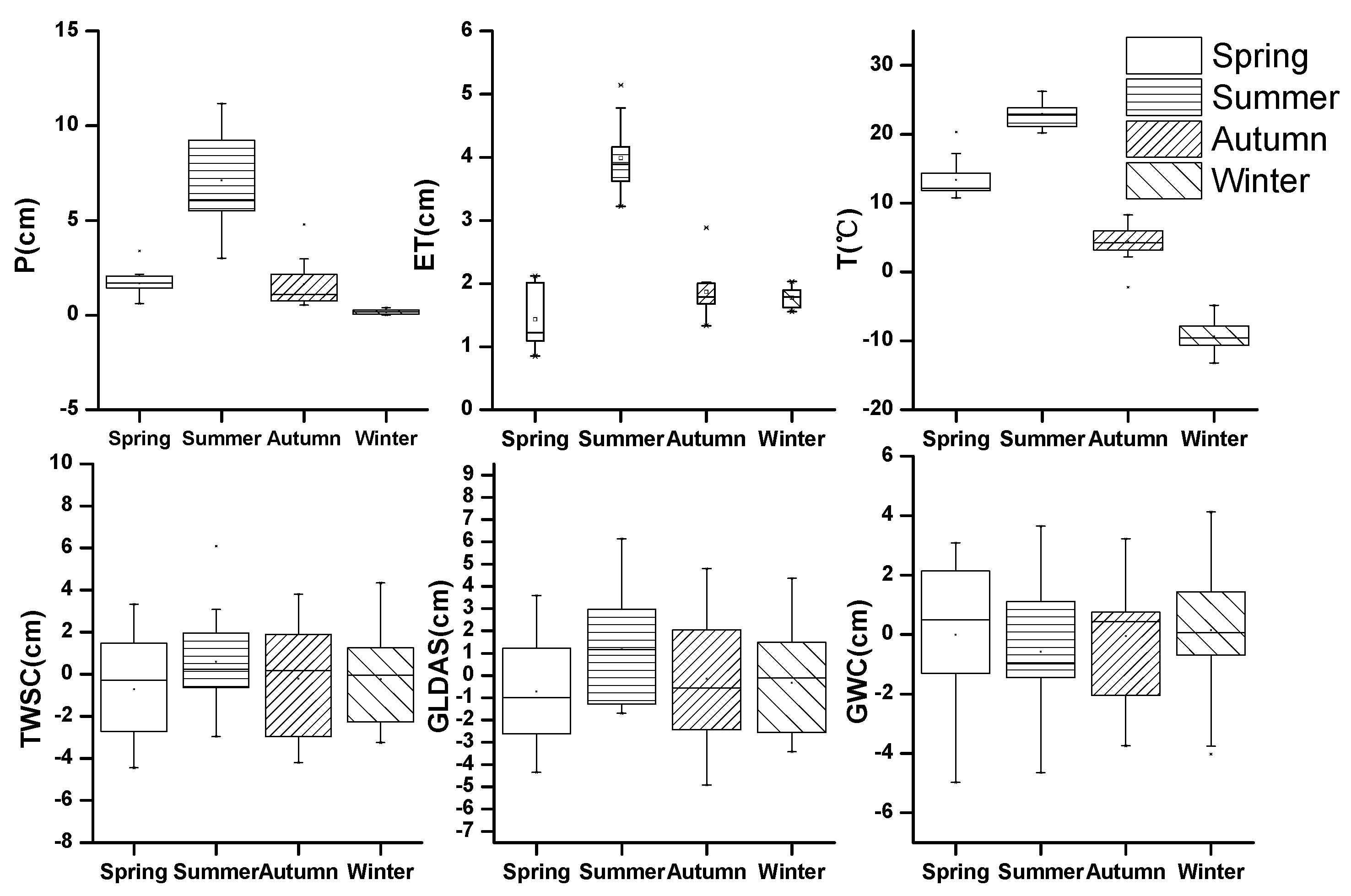
3.1. Changes of Hydrological Factors over Time

The observations in Figure 2 showed that hydrological factors changed annually. In general, total annual precipitation (P) and evapotranspiration (ET) increased by 0.05 cm/yr. and 0.01 cm/yr., respectively, on average from 2002 to 2014. P showed a slightly greater rate of increase after 2008 than before. During 2002 and 2014, mean annual temperature (T) decreased on average by −0.05 °C/yr. Terrestrial water storage change (TWSC) increased from 2002 to 2005 and decreased significantly from 2006 to the beginning of 2012, which led to a value that was approximately 6 cm less than the mean of the whole obtained TWSC series (Figure 2b). TWSC increased again after 2012 and reached a value equivalent to the average of the whole series’ mean. Monthly soil moisture change (SMC), snow water equivalent change (SWEC), total canopy water storage change (TCWSC) obtained from GLDAS, fluctuated from 2002 to 2014 (Figure 2c). SMC in the study area had obvious seasonal variations and ranged from −5.24~8.26 cm, and this parameter was sensitive to changes in regional water resources. There were significant differences in the time series of SWEC, which generally reached a peak in December. In the process of freezing and thawing in spring, the value decreased slowly until the end of April. The maximum value of SWEC was 1.36 cm in December 2012. The TCWSC value reached the maximum in July or August in summer and showed an upward trend in the study area, with a range from −0.01 to 0.01 mm. Analysis of TWSC and auxiliary data-Global Land Data Assimilation System (GLDAS = SMC + SWEC + TCWSC) showed that temporal patterns groundwater change (GWC) could be described based on time series analysis (Figure 2d). GWC in the study time showed a clear decreasing trend at rate of −0.43 cm/yr., and especially experienced a significant decrease from 2007 to 2012 at a rate of −0.99 cm/yr. Furthermore, TWSC lagged behind other factors at the time scale, e.g., P, SMC and so on in Figure 2.
In addition to annual changes, hydrological factors changed seasonally as well in Figure 3. P, ET and T values showed similar seasonal change patterns, with a high peak values occurring in summer and a low peak value occurring in winter. TWSC and GLDAS increased from spring to summer and then decreased from autumn to winter. A similar change trend was observed for TWSC and GLDAS with P, T and ET, indicating that there was an interaction between these factors. However, a lag effect was also observed, which required further quantitative analysis. The inter-annual trend of GWC showed a continuous downward trend, gradually decreasing from the maximum value in spring to the minimum value in winter, indicating that the annual groundwater storage gradually decreased, especially in summer where this phenomenon was more obvious.

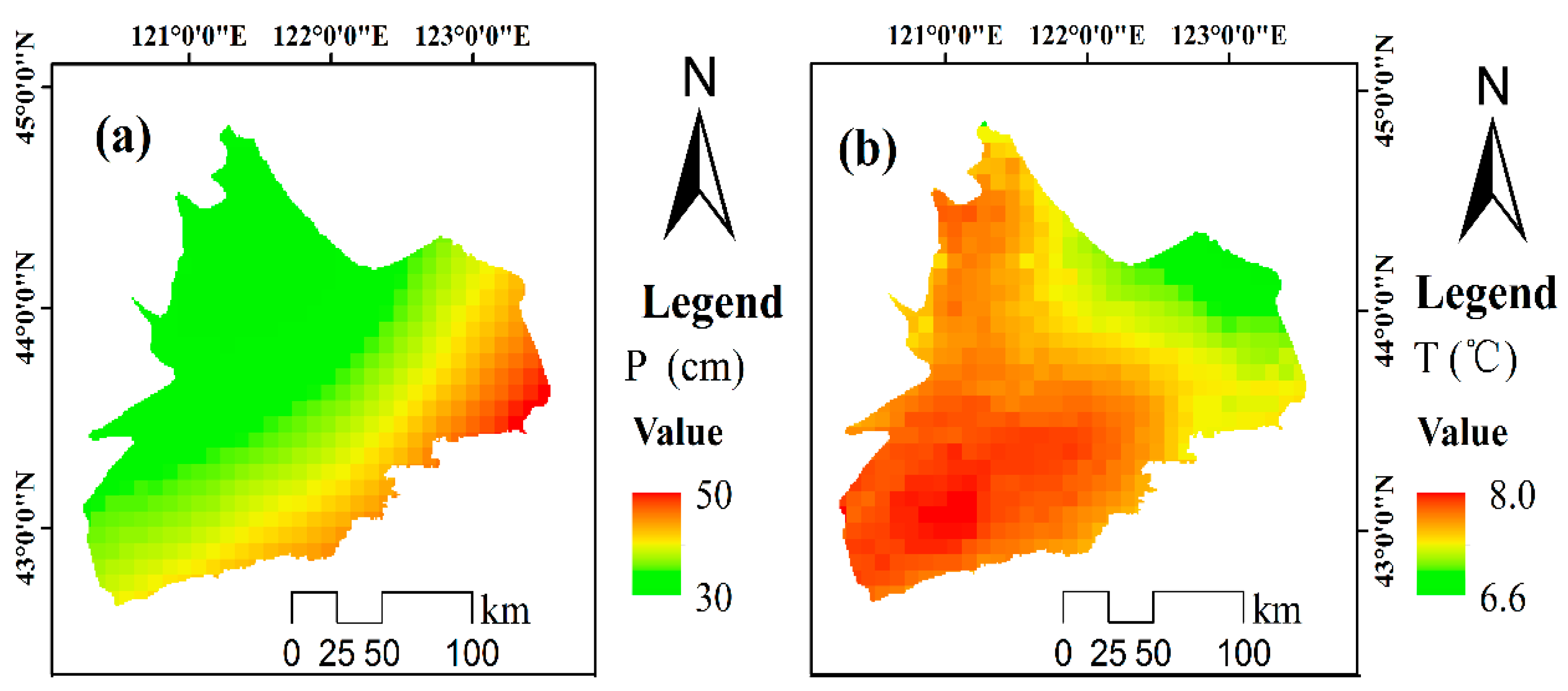
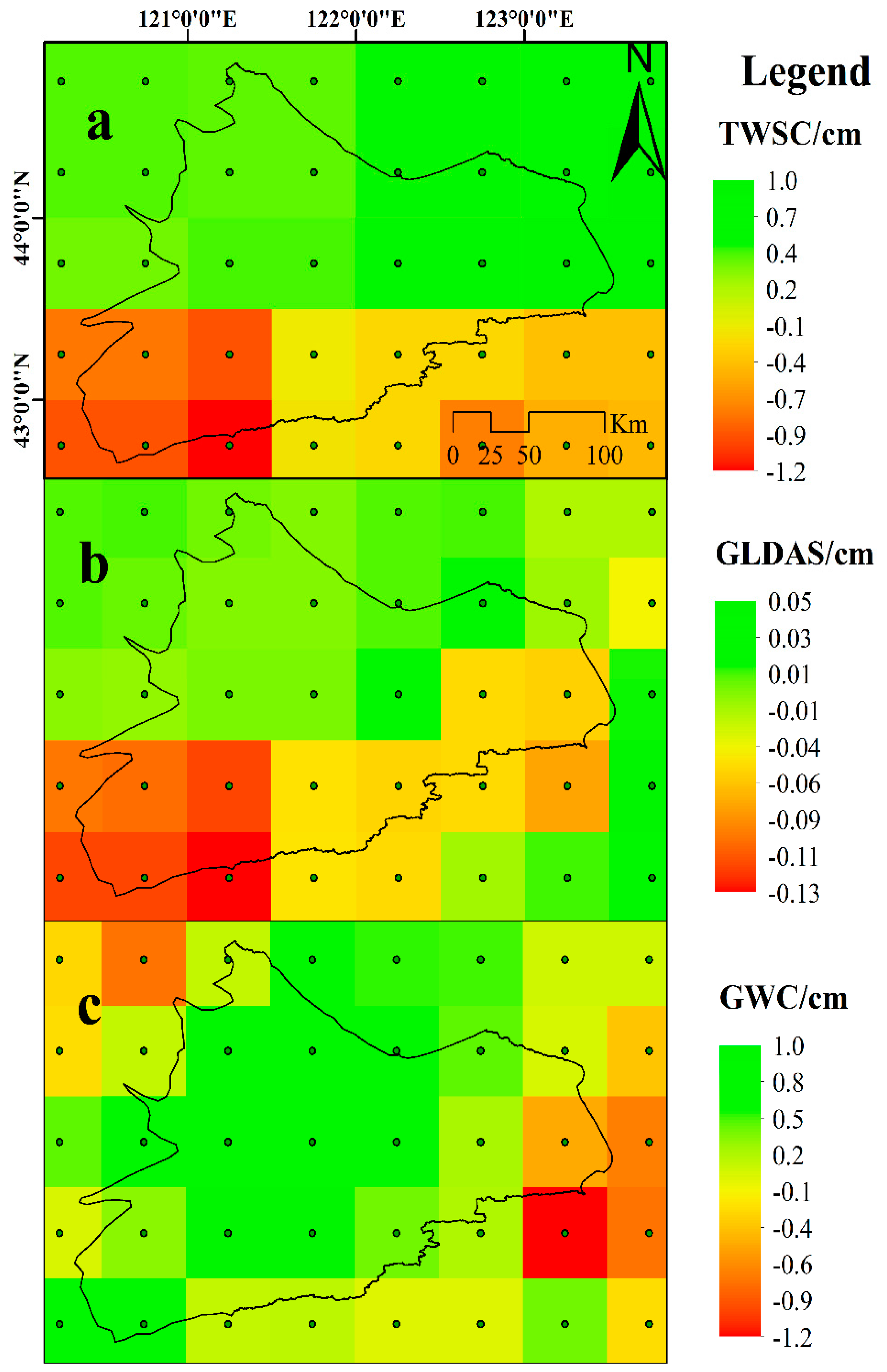
3.2. Spatial Distribution of Annual Hydrological Factors

3.2.1. Situ Observation of Hydrological Factors

The in-situ observations of hydrological factors between 2002 and 2014 showed that the mean annual P increased from northwestern to southeastern areas, with an average value of 37.2 cm, while the mean annual T decreased from southwestern to northeastern areas, with an average value of 7.5 °C (Figure 4a,b). This result indicated that hydrological and meteorological factors in the study area have significant spatial heterogeneity, while spatial distributions between P and T were different.

3.2.2. Hydrological Factors from Satellite Data

TWSC data observed from the satellite in the study area showed a decreasing trend from northeast to southwest on the whole in Figure 5. The northern and central region were in a state of accumulation, while the southern region was in a state of deficit with a relatively obvious decreasing trend (Figure 5a). Based on GLDAS data, SMC, SWEC and TCWS showed equivalent water increases, as shown in Figure 5b. Spatial distribution of GLDAS was similar to that of TWSC, indicating that there was an interaction between these parameters. The GWC value showed a slight surplus state in most area of XRB, which ranged from −1.2 to 1.0 cm (Figure 5c).

3.3. Spatiotemporal Variations of Normalized Difference Vegetation Index (NDVI)

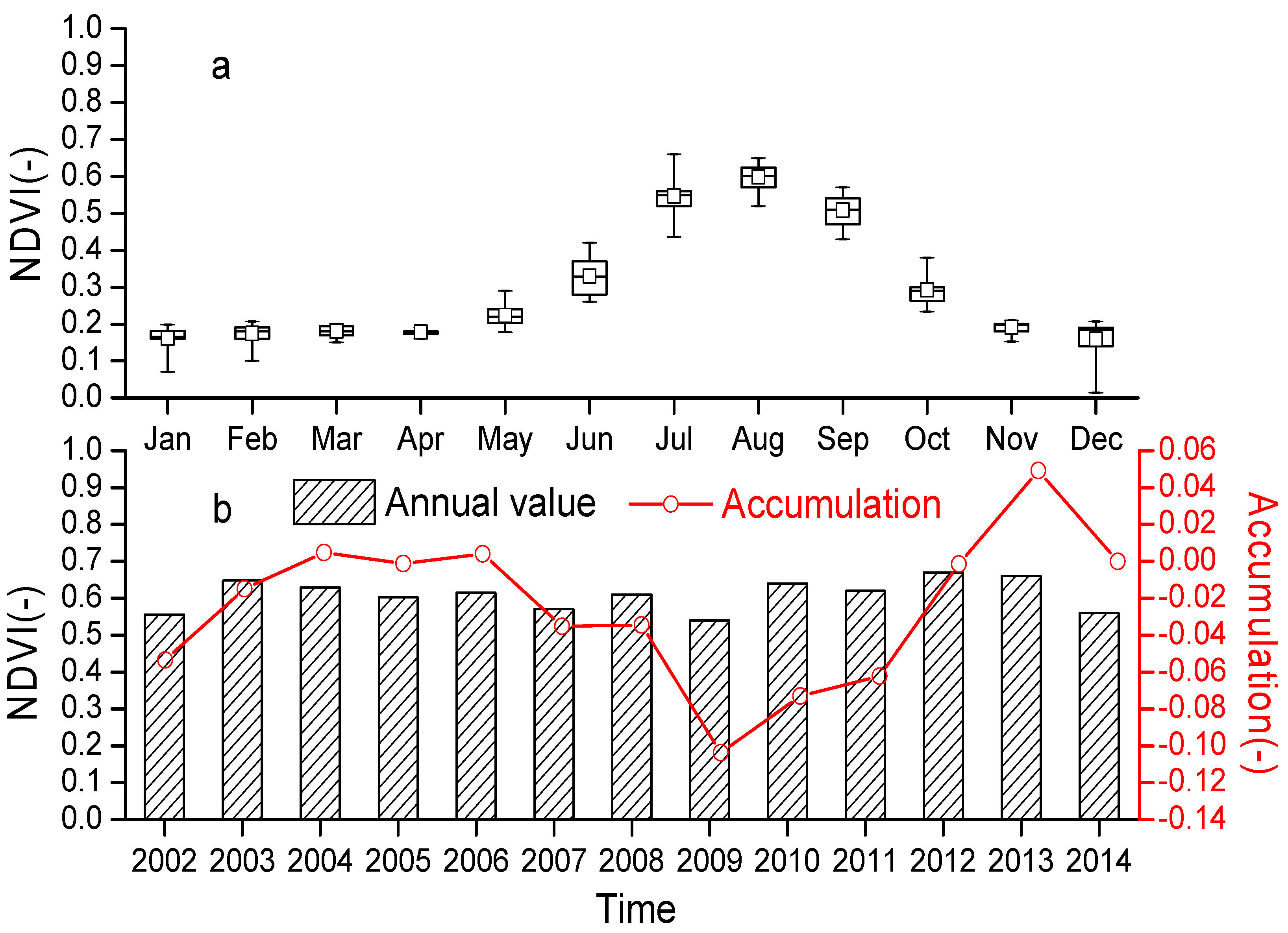
3.3.1. Temporal Variation

Similar to other areas in northern China, NDVI had apparent seasonal variation, and showed an upward trend during 2002 and 2014 in Figure 6. The NDVI increased from May to the most vigorous growing season in July and August, and it then decreased to the minimum level in November and remained almost unchanged until the following April, with a range of the NDVI of 0.16~0.19 (Figure 6a). In addition, NDVI showed a single peak change during the year in Figure 6a as well as hydrological factors in the study area in Figure 2a, meaning that there were relationships between them. Furthermore, the annual value of NDVI increased slightly at a rate of 0.001 yr−1 from 2002 to 2014 in Figure 6b. The analysis of the cumulative anomaly method showed that NDVI decreased from 2002 to 2009 and then increased again (Figure 6b). This change trend was also consistent with the change trend of hydrological factors in the study area (Figure 2b,d), indicating that water factors in semiarid areas, especially groundwater, may be the main factors affecting vegetation changes.

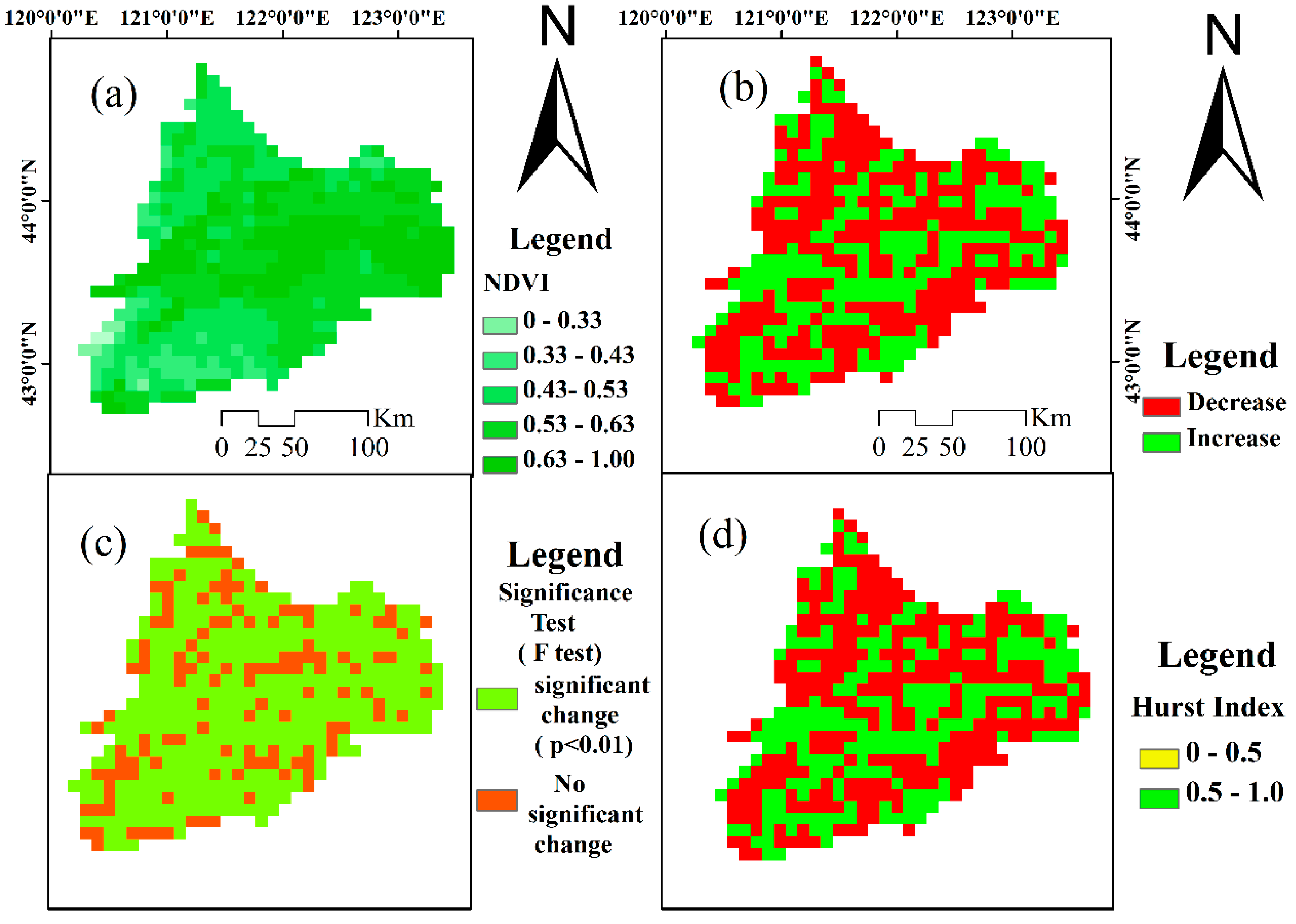
3.3.2. Spatial Variations

Figure 7 showed that the spatial distribution of NDVI was heterogeneous in the area. NDVI value was lower in the southwestern area, with a range of 0.0~0.33, than in the central belt from west to east (Figure 7a). NDVI was greater along the rivers, which ranged from 0.63~1.00, than other parts, which ranged from 0.0~0.63. Furthermore, the annual value of NDVI decreased over 63.2% of the area at a rate of −0.008~0.0 a−1, while 36.8% of the area showed an increase in the NDVI at rate of 0~0.02 a−1 (Figure 7b). F test results suggested that significant variance area accounted for 89.3% of the whole area and was mostly distributed in areas with a relatively lower NDVI value (Figure 7c). Significant variance was not observed in cultivated areas along rivers. The Hurst index (0.06~0.97) indicated that in 55.7% of the area, particularly in areas with a decreasing NDVI trend, the variance trend was continuously maintained for a long time while the remaining 44.3% of the area would show fluctuations (Figure 7d).

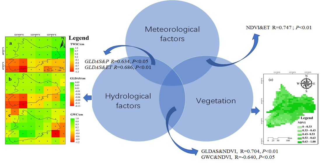
3.4. Relationships between Hydrological Factors

The value of P was highly related to ET, with a correlation coefficient of 0.685 (P < 0.01). TWSC had a significant correlation (R = 0.680, P < 0.05) with GWC, as compared to GLDAS in Table 2, indicating that TWSC mainly consisted of GWC in the area. GLDAS had a significant and positive correlation with P (R = 0.634, P < 0.05) and ET (R = 0.686, P < 0.01), meaning that a higher P rate corresponded to more SMC. Significant positive correlation was observed between T and GWC (R = 0.680, P < 0.05), which indicated that water demand of plants increased as T increased in XRB and groundwater was the main source of water in semiarid area and changed significantly. In summary, there are complex correlations among regional hydrological elements.
P is not the only one of the most important factors underlying the interactions among the hydrological cycle but also the key variable in the water resources in semiarid areas. It accounted for approximately 75% of total water resource recharge in normal years and approximately 57% of recharge in dry years in study area [11]. A lag time of P infiltration is observed based on GLDAS and GWC. Lag time is usually represented in hydrological forecasts based on P in the hydrological equilibrium [51]. Table 3 showed their relationships between TWSC, GLDAS and GWC and P and ET, which were analyzed to determine lag times. The results showed that TWSC and GLDAS had significant correlation (P < 0.05) with P at different lag periods, i.e., a one-month time lag occurred (R = 0.312, P < 0.05). Moreover, these parameters were significantly and positively correlated with the ET in the current month (R = 0.276, P < 0.05) and one month prior (R = 0.276, P < 0.05) but not positively correlated (p > 0.01) with the ET two to three months later. This finding suggested that the P and ET in the current month and one-month prior could significantly affect the TWSC and GLDAS. Meanwhile, P and ET did not have correlation (P > 0.05) with GWC, which might be related to the considerable depth of groundwater table due to overexploitation, long time period for infiltration to recharge groundwater or lack of infiltration recharge of groundwater due to ET. As a result of this, P and ET were increasingly less sensitive to GWC.

3.5. Relationships between Hydrological Factors and NDVI

To obtain better understanding of relationships between hydrological factors and NDVI, correlation analysis was carried out. As shown in Table 4, the results showed that ET and GLDAS were significantly and positively correlated with NDVI (R = 0.747 and 0.704; P < 0.01) in the growing season (May-Oct) of vegetation. Correlation coefficient between NDVI and GWC in the growing season was significantly negatively correlated (R = −0.64, P < 0.05), indicating that groundwater represents an important water source for vegetation growth in the XRB. T and TWSC had no effect on the growth of vegetation in each season, and their correlation coefficients did not pass the significance test. In summary, ET, GLDAS and GWC could be the major hydrological parameters that affect vegetation dynamics in the growing season.

4. Discussion

4.1. Dynamics of Hydroecological Elements in Semiarid Area

Water for agricultural irrigation relies heavily on groundwater due to shortages of surface water in study area [47], and reports have indicated that more than 80% of the water use was from groundwater [11]. Spatiotemporal variation and distribution characteristics of the hydrological factors were determined by multiple satellite data, which have been widely used as effective approaches for detecting the hydrological dynamics in ecotones in semiarid areas. Combined with the analysis results of climate change in the study area, spatial distribution of precipitation (P) and temperature (T) was uneven, as shown in Figure 4 and presented a decreasing and increasing trend from the southeast to the northwest, respectively. The results showed that, on the spatial scale, terrestrial water storage change (TWSC) results based on JPL satellite data and auxiliary data-Global Land Data Assimilation System (GLDAS = SMC + SWEC + TCWSC) values were also closely related to P and T. Application of the multi-satellite data would represent an effective approach to monitoring and modeling the dynamics of groundwater change (GWC). Our result confirms that the environment changes have occurred in the semiarid area and that they can be related to dynamics of hydrogeological elements were easily observable and measurable through satellite images. Through correlation analysis, there are complex relationships among regional hydrological elements in Table 2. Furthermore, soil moisture change (SMC) and snow water equivalent change (SWEC) obtained from the GLDAS data played an important role in the hydrological cycle in the area. The SWEC not only affected the surface runoff, groundwater recharge, and SMC in the spring [52,53,54], but also indicated the snow cover in the winter and the accumulated air temperature in the spring (Figure 2). SMC could even directly reflect the vegetation growth in growing season, and predict the GWC [55,56]. SMC was higher for irrigated land than grassland in the vegetation growth season (Figure 5). In particular, SMC and GWC directly affected the local hydrologic cycle, which could be used to optimize the management and utilization of water resources and improve vegetation growth. However, compared to other areas [57], the response between P and GWC was increasingly insensitive in the study area with a lag period of one month. There are many reasons for this phenomenon, but anthropic factors [58], e.g., irrigation and overexploitation of groundwater, have thickened the vadose zone of soil, and the relationship between P and groundwater, which is is becoming more and more complex.
While the application of the satellite data can significantly improve the level of water resources assessment in this area, there are still some deficiencies, such as time scale (monthly), spatial resolution (0.5 degree) and data accuracy verification, which have a significant impact on the research results of small and medium-sized watersheds, e.g., the correlation strength between them and other environmental molecules is very poor, only the correlation can be considered. Therefore, how to combine the limited water resources monitoring information with new methods, new technologies and new achievements to carry out effective regional water resources management has become a practical problem demand of relevant departments of water resource management.

4.2. Impacts of Hydrological Factors on Vegetation

Hydrological factors played a controlling role in terrestrial ecosystems [59,60]. Field survey in July of 2015 and August of 2016 and normalized difference vegetation index (NDVI) value showed that the northern part of the study was dominated by grassland with medium vegetation coverage, the middle part was dominated by cultivated land with high vegetation coverage, and the southern part was dominated by sandy land with low vegetation coverage. The results in the paper showed that ET, GLDAS and GWC could be the major hydrological parameters that affect the vegetation dynamics in the growing season. The northeastern XRB included grassland with some small rivers with high terrain and vegetation coverage, and it was affected by snow melt water in the spring as well as rainfall. As a result, GLDAS and TWSC showed a cumulative trend with higher values in the northern piedmont plain than in other areas, indicating that the piedmont plain had basically maintained its original ecology and was rarely affected by human activities. Change of GWC in the central part of the study area, which is a flat, wide area of cultivated land, was relatively reduced as shown in Figure 5c. Therefore, irrigation had a significant impact on regional SMC and even affected regional water resource reserves [61], which indicated that the GWC might be affected by human activities, such as the expansion of cultivated land area [62] and overexploitation and utilization of groundwater [63]. TWSC in the southwest of the study area showed a decreasing trend (Figure 5a) [64]. Major land use types in the area consisted of typical steppe, meadow steppe, and cropland in Figure 1, and vegetation growth in these areas was dependent on ET (R = 0.747, P < 0.05) and GLDAS (R = 0.704, P < 0.05) which was mainly consisted of SMC. However, in summer and the vegetation growing season, P and NDVI were positively correlated, although the occurrence of this phenomenon is mainly related to the serious desertification of the local surface and the inability of the soil to store water correlation coefficient failed the significance test (Table 3) which indicated that lower P did not have a significant effect on the vegetation in the semiarid area [65]. NDVI, as an intuitive indicator of vegetation growth, plays a fundamental role in reflecting the characteristics of vegetation growth and distribution. However, NDVI is hardly enough to explain vegetation changes, such as vegetation height, density and so on. Furthermore, grassland will often give a stronger NDVI value than forest but the effect on ET and GWC are very different. In future, more indexes related to water should be used in the study of regional hydroecological processes.

5. Conclusions

Using multiple satellite data, the spatiotemporal changes of hydrological elements in semiarid areas from 2002 to 2014 and their effects on vegetation were analyzed in this paper. The main conclusions are as follows.
(1) Analysis of spatiotemporal characteristics of hydrological elements showed that the hydrological process in the study area has changed significantly. Annual variations of precipitation (P), evapotranspiration (ET) and temperature (T) were all in the form of a single peak, and the interannual variation law was slightly different, with rates of 0.05 cm/yr., 0.01 cm/yr. and −0.05°C/yr., respectively. Terrestrial water storage change (TWSC) showed a fluctuating trend, with initial increase, then decrease, and finally an increase, which was consistent with the change trend of soil moisture change (SMC). Groundwater change (GWC) showed a decreasing trend at a rate of −0.17 cm/yr.
(2) Complex correlations occurred among regional hydrological elements. P and ET were significantly correlated (R = 0.685, P < 0.01) and had a greater impact on the GLDAS (R = 0.634, P < 0.05 and R = 0.686, P < 0.01) than on the TWSC and GWC. GWC is an important component of the TWSC in the region (R = 0.680, P < 0.05), and it was more sensitive to the T response (R = 0.570, P < 0.05). Furthermore, P would lead to greater TWSC and GLDAS values when P preceded the TWSC by one month, whereas smaller changes would be observed when P preceded these parameters by two months. The time lag of the GLDAS that was influenced by P was more obvious than that of the TWSC. The TWSC and GLDAS were significantly and positively correlated with the ET in the current month and one month prior and not positively correlated with the ET two to three months later. Due to overexploitation, P and ET did not have any effect on the GWC.
(3) Normalized difference vegetation index (NDVI) had obvious seasonal variations and showed an upward trend at a rate of 0.001 yr−1 during 2002 and 2014. Spatial distribution of NDVI was heterogeneous in study area. NDVI decreased by 63.2% of the area at rate of −0.008~0.0 yr−1. The area showing significant variance accounted for 89.3% of the whole area, and 55.7% of the area would maintain the variance trend continuously for a long time, with these areas mainly showing decreasing NDVI change trends. However, other 44.3% area would show fluctuations. Hydrological factors play a controlling role on terrestrial ecosystems. In growing season, ET, GLDAS and GWC were the parameters that limited vegetation growth, and they were more important than other factors in XRB.
Application of satellite data could significantly improve the water assessment capability in semiarid areas and could be used for regional water resource and eco-environment management in semiarid areas. Hydrological factors, such as TWSC, SM and GWC, spatiotemporal dynamic and their correlations were successfully determined and analyzed in this study. Impacts of hydrological change on NDVI were also identified based on the analysis. These results will help to understand regional hydroecological processes, and also provide a scientific basis for local environmental management.

Author Contributions

Methodology, S.Z.; software, B.S.; data curation, Y.Z.; writing—original draft preparation, Y.Z.; writing—review and editing, P.L. All authors have read and agreed to the published version of the manuscript.

Funding

This research was funded by National Key R&D Program of China (2018YFE0103800), Ministry of Water Resources Public Welfare Special Scientific Research Project—Semi-arid Zone Water Cycle and Water Ecological Security Key Technology Research (number 201501031), National Natural Science Foundation of China (51779118, 51669021, 51869020), Fundamental Research Funds for the Central Universities, CHD (300102299302, 300102299102, 300102299104), One Hundred Talent Plan of Shaanxi Province, International Collaborative Research of Disaster Prevention Research Institute of Kyoto University(2019W-02), Excellent Projects for Science and Technology Activities of Overseas Staff in Shaanxi Province (2018038), Yan’an University Project (YDBK2017-19, YDBK2019-35, YDBK2019-36), and Yan’an Science and Technology Bureau (project 2018KS-02).

Acknowledgments

The authors would like to thank the Editors and the anonymous reviewers for their crucial comments, which improved the quality of this paper.

Conflicts of Interest

The authors declare no conflict of interest.

References

  1. Huang, J.; Zhang, W.; Zuo, J.; Fu, C.; Chou, J.; Feng, G.; Yuan, J.; Zhang, L.; Wang, S.; Zuo, H.; et al. Development of the semi-arid climate and environment research observatory over Loess Plateau. Adv. Atmos. Sci. 2008, 25, 906–921. [Google Scholar] [CrossRef]
  2. Nielsen, U.N.; Ball, B.A. Impacts of altered precipitation regimes on soil communities and biogeochemistry in arid and semi-arid ecosystems. Glob. Chang. Biol. 2015, 21, 1407–1421. [Google Scholar] [CrossRef] [PubMed]
  3. Wu, Y.; Liu, T.X.; Paredes, P.; Duan, L.M.; Wang, H.Y.; Wang, T.S.; Pereira, L.S. Ecohydrology of groundwater-dependent grasslands of the semi-arid Horqin sandy land of inner Mongolia focusing on evapotranspiration partition. Ecohydrology 2016, 9, 1052–1067. [Google Scholar] [CrossRef]
  4. Villalobos-Vega, R.; Salazar, A.; Miralles-Wilhelm, F.; Haridasan, M.; Franco, A.C.; Goldstein, G.; Wesche, K. Do groundwater dynamics drive spatial patterns of tree density and diversity in Neotropical savannas? J. Veg. Sci. 2014, 25, 1465–1473. [Google Scholar] [CrossRef]
  5. Dai, X.Q.; Shi, H.B.; Li, Y.S.; Ouyang, Z.; Huo, Z.L. Artificial neural network models for estimating regional reference evapotranspiration based on climate factors. Hydrol. Process. 2009, 23, 442–450. [Google Scholar] [CrossRef]
  6. He, D.; Liu, Y.; Pan, Z.; An, P.; Wang, L.; Dong, Z.; Zhang, J.; Pan, X.; Zhao, P. Climate change and its effect on reference crop evapotranspiration in central and western Inner Mongolia during 1961–2009. Front. Earth Sci. 2013, 7, 417–428. [Google Scholar] [CrossRef]
  7. Zhang, F.; Zhou, G.S.; Wang, Y.; Yang, F.L.; Nilsson, C. Evapotranspiration and crop coefficient for a temperate desert steppe ecosystem using eddy covariance in Inner Mongolia, China. Hydrol. Process. 2012, 26, 379–386. [Google Scholar] [CrossRef]
  8. Miao, L.; Jiang, C.; Xue, B.; Liu, Q.; He, B.; Nath, R.; Cui, X. Vegetation dynamics and factor analysis in arid and semi-arid Inner Mongolia. Environ. Earth Sci. 2014, 73, 2343–2352. [Google Scholar] [CrossRef]
  9. Li, S.G.; He, Z.Y.; Chang, X.L.; Harazono, Y.; Oikawa, T.; Zhao, H.L. Grassland desertification by grazing and the resulting micrometeorological changes in Inner Mongolia. Agric. For. Meteorol. 2000, 102, 125–137. [Google Scholar]
  10. Zunya, W.; Yihui, D.; Jinhai, H.; Jun, Y. An updating analysis of the climate change in china in recent 50 years. Acta Meteorol. Sin. 2004, 62, 228–236. [Google Scholar]
  11. Zhong, Y.L.; Zhong, M.; Feng, W.; Zhang, Z.Z.; Shen, Y.C.; Wu, D.C. Groundwater Depletion in the West Liaohe River Basin, China and Its Implications Revealed by GRACE and In Situ Measurements. Remote Sens. 2018, 10, 493. [Google Scholar] [CrossRef] [Green Version]
  12. Li, B.; Yu, W.; Wang, J. An Analysis of Vegetation Change Trends and Their Causes in Inner Mongolia, China from 1982 to 2006. Adv. Meteorol. 2011, 2011, 13–30. [Google Scholar] [CrossRef] [Green Version]
  13. Huang, J.; Sun, S.; Xue, Y.; Zhang, J. Changing characteristics of precipitation during 1960–2012 in Inner Mongolia, northern China. Meteorol. Atmos. Phys. 2014, 127, 257–271. [Google Scholar] [CrossRef]
  14. Yang, H.S.; Liu, J.; Liang, H.Y. Change characteristics of climate and water resources in west Liaohe River Plain. J. Appl. Ecol. 2009, 20, 84–90. (In Chinese) [Google Scholar]
  15. Gao, Z.; He, J.; Dong, K.; Bian, X.; Li, X. Sensitivity study of reference crop evapotranspiration during growing season in the West Liao River basin, China. Theor. Appl. Climatol. 2015, 124, 865–881. [Google Scholar] [CrossRef]
  16. Schaffrath, D.; Bernhofer, C. Variability and distribution of spatial evapotranspiration in semiarid Inner Mongolian grasslands from 2002 to 2011. Springerplus 2013, 2, 547. [Google Scholar] [CrossRef] [Green Version]
  17. Liu, X.P.; He, Y.H.; Zhao, X.Y.; Zhang, T.H.; Li, Y.L.; Yun, J.Y.; Wei, S.L.; Yue, X.F. The response of soil water and deep percolation under Caragana microphylla to rainfall in the Horqin Sand Land, northern China. Catena 2016, 139, 82–91. [Google Scholar] [CrossRef]
  18. Yao, S.X.; Zhao, C.C.; Zhang, T.H.; Liu, X.P. Response of the soil water content of mobile dunes to precipitation patterns in Inner Mongolia, northern China. J. Arid. Environ. 2013, 97, 92–98. [Google Scholar] [CrossRef] [Green Version]
  19. Zhu, L.; Gong, H.L.; Dai, Z.X.; Xu, T.B.; Su, X.S. An integrated assessment of the impact of precipitation and groundwater on vegetation growth in arid and semiarid areas. Environ. Earth Sci. 2015, 74, 5009–5021. [Google Scholar] [CrossRef] [Green Version]
  20. Feng, W.; Zhong, M.; Lemoine, J.M.; Biancale, R.; Hsu, H.T.; Xia, J. Evaluation of groundwater depletion in North China using the Gravity Recovery and Climate Experiment (GRACE) data and ground-based measurements. Water Resour. Res. 2013, 49, 2110–2118. [Google Scholar] [CrossRef]
  21. Wahr, J.; Molenaar, M.; Bryan, F. Time variability of the Earth’s gravity field: Hydrological and oceanic effects and their possible detection using GRACE. J. Geophys. Res. Solid Earth 1998, 103, 30205–30229. [Google Scholar] [CrossRef]
  22. Chen, Z.; Jiang, W.; Wu, J.; Chen, K.; Deng, Y.; Jia, K.; Mo, X. Detection of the spatial patterns of water storage variation over China in recent 70 years. Sci. Rep. 2017, 7, 6423. [Google Scholar] [CrossRef] [PubMed] [Green Version]
  23. Yang, P.; Xia, J.; Zhan, C.; Qiao, Y.; Wang, Y. Monitoring the spatio-temporal changes of terrestrial water storage using grace data in the Tarim river basin between 2002 and 2015. Sci. Total Environ. 2017, 595, 218–228. [Google Scholar] [CrossRef] [PubMed]
  24. Yeh, P.J.-F.; Swenson, S.C.; Famiglietti, J.S.; Rodell, M. Remote sensing of groundwater storage changes in illinois using the gravity recovery and climate experiment (grace). Water Resour. Res. 2006, 42, 4. [Google Scholar] [CrossRef]
  25. Singh, A.K.; Tripathi, J.N.; Kotlia, B.S.; Singh, K.K.; Kumar, A. Monitoring groundwater fluctuations over india during indian summer monsoon (ism) and northeast monsoon using grace satellite: Impact on agriculture—Sciencedirect. Quat. Int. 2019, 507, 342–351. [Google Scholar] [CrossRef]
  26. Han, Z.; Huang, S.; Huang, Q.; Leng, G.; Wang, H.; He, L.; Fang, W. Assessing grace-based terrestrial water storage anomalies dynamics at multi-timescales and their correlations with teleconnection factors in yunnan province, china. J. Hydrol. 2019, 574, 836–850. [Google Scholar] [CrossRef]
  27. Lv, M.; Ma, Z.; Li, M.; Zheng, Z. Quantitative Analysis of Terrestrial Water Storage Changes under the Grain for Green Program in the Yellow River Basin. J. Geophys. Res. Atmos. 2019, 124, 1336–1351. [Google Scholar] [CrossRef]
  28. Zhang, Q.; Singh, V.P.; Sun, P.; Chen, X.; Zhang, Z.X.; Li, J.F. Precipitation and streamflow changes in China: Changing patterns, causes and implications. J. Hydrol. 2011, 410, 204–216. [Google Scholar] [CrossRef]
  29. Long, W.H.; Chen, H.H.; Li, Z.; Pan, H.J. Evaluation of the groundwater intrinsic vulnerability in West Liaohe plain, Inner Mongolia, China. Geological Bulletin of China. Geol. Bull. China 2010, 29, 598–602. [Google Scholar]
  30. Zhu, Y.H.; Zhang, S.; Sun, B.; Yan, L.; Wang, Y. Relationship of dominant herbaceous plant species and groundwater depth in tongliao plain, northwestern china. Appl. Ecol. Environ. Res. 2019, 17, 15363–15374. [Google Scholar] [CrossRef]
  31. Jia, X.; Lee, H.F.; Zhang, W.C.; Wang, L.; Sun, Y.G.; Zhao, Z.J.; Yi, S.W.; Huang, W.B.; Lu, H.Y. Human-environment interactions within the West Liao River Basin in Northeastern China during the Holocene Optimum. Quat. Int. 2016, 426, 10–17. [Google Scholar] [CrossRef]
  32. Hutchinson, M.F. Interpolation of rainfall data with thin plate smoothing splines I. two-dimensional smoothing of data with shortrange correlation. Geogr. Inf. Decis. Anal. 1998, 2, 153–167. [Google Scholar]
  33. Mu, Q.; Heinsch, F.A.; Zhao, M.; Running, S.W. Development of a global evapotranspiration algorithm based on MODIS and global meteorology data. Remote Sens. Environ. 2007, 111, 519–536. [Google Scholar] [CrossRef]
  34. Mu, Q.; Zhao, M.; Heinsch, F.A.; Liu, M.; Tian, H.; Running, S.W. Evaluating water stress controls on primary production in biogeochemical and remote sensing based models. J. Geophys. Res. Biogeosci. 2015, 112, 863–866. [Google Scholar] [CrossRef] [Green Version]
  35. Ouyang, W.; Liu, B.; Wu, Y.Y. Satellite-based estimation of watershed groundwater storage dynamics in a freeze-thaw area under intensive agricultural development. J. Hydrol. 2016, 537, 96–105. [Google Scholar] [CrossRef]
  36. Feixiao, G.; Zhongmiao, S.; Feilong, R.; Yun, X. Comparison and Analysis of Different Mascon Model Results. J. Geod. Geodyn. 2019, 39, 1022–1026. [Google Scholar]
  37. Cheng, M.; Tapley, B.D. Variations in the Earth’s Oblateness during the Past 28 Years. J. Geophys. Res. Solid Earth 2004, 109. [Google Scholar] [CrossRef]
  38. Swenson, S.; Chambers, D.; Wahr, J. Estimating Geocenter Variations from a Combination of GRACE and Ocean Model Output. J. Geophys. Res. Solid Earth 2008, 113. [Google Scholar] [CrossRef] [Green Version]
  39. Geruo, A.; Wahr, J.; Zhong, S. Computations of the Viscoelastic Response of a 3-D Compressible Earth to Surface Loading: An Application to Glacial Isostatic Adjustment in Antarctica and Canada. Geophys. J. Int. 2013, 192, 557–572. [Google Scholar]
  40. Watkins, M.M.; Wiese, D.N.; Yuan, D.-N.; Boening, C.; Landerer, F.W. Improved Methods for Observing Earth’s Time Variable Mass Distribution with GRACE Using Spherical Cap Mascons. J. Geophys. Res. Solid Earth 2015, 120, 2648–2671. [Google Scholar]
  41. Rodell, M.; Chen, J.; Kato, H.; Famiglietti, J.S.; Nigro, J.; Wilson, C.R. Estimating groundwater storage changes in the Mississippi River basin (USA) using GRACE. Hydrogeol. J. 2006, 15, 159–166. [Google Scholar] [CrossRef] [Green Version]
  42. Save, H.; Bettadpur, S.; Tapley, B.D. High-resolution CSR GRACE RL05 mascons. J. Geophys. Res. Sol. Earth 2016, 121, 7547–7569. [Google Scholar] [CrossRef]
  43. Holger, S.; Patrick, W.; Hansheng, W. Determination of the Earth’s structure in Fennoscandia from GRACE and implications for the optimal post-processing of GRACE data. Geophys. J. Int. 2010, 182, 1295–1310. [Google Scholar]
  44. Rodell, M.; Velicogna, I.; Famiglietti, J.S. Satellite-based estimates of groundwater depletion in India. Nature 2009, 460, 999–1002. [Google Scholar] [CrossRef] [Green Version]
  45. Nanteza, J.; De Linage, C.R.; Thomas, B.F.; Famiglietti, J.S. Monitoring groundwater storage changes in complex basement aquifers: An evaluation of the grace satellites over eastafrica. Water Resour. Res. 2016, 52, 9542–9564. [Google Scholar]
  46. Long, D.; Yang, Y.; Wada, Y.; Hong, Y.; Liang, W.; Chen, Y.; Chen, L. Deriving scaling factors using a global hydrological model to restore. J. Remote Sens. Environ. 2015, 168, 177–193. [Google Scholar] [CrossRef]
  47. Holben, B.N. Characteristics of maximum-value composite images from temporal AVHRR data. Int. J. Remote Sens. 1986, 7, 1417–1434. [Google Scholar] [CrossRef]
  48. Jiang, L.; Bao, A.; Guo, H.; Ndayisaba, F. Vegetation dynamics and responses to climate change and human activities in central Asia. Sci. Total Environ. 2017, 599–600, 967–980. [Google Scholar] [CrossRef]
  49. Hou, W.; Hou, X. Spatial–temporal changes in vegetation coverage in the global coastal zone based on gimms ndvi3g data. Int. J. Remote Sens. 2019, 41, 1118–1138. [Google Scholar] [CrossRef]
  50. Tong, S.; Zhang, J.; Bao, Y.; Lai, Q.; Lian, X.; Li, N.; Bao, Y. Analyzing vegetation dynamic trend on the Mongolian Plateau based on the Hurst exponent and influencing factors from 1982–2013. J. Geogr. Sci. 2018, 28, 595–610. [Google Scholar] [CrossRef] [Green Version]
  51. Thompson, S.E.; Harman, C.J.; Troch, P.A.; Brooks, P.D.; Sivapalan, M. Spatial scale dependence of ecohydrologically mediated water balance partitioning: A synthesis framework for catchment ecohydrology. Water Resour. Res. 2011, 47, W00J03. [Google Scholar] [CrossRef]
  52. Abelen, S.; Seitz, F. Relating satellite gravimetry data to global soil moisture products via data harmonization and correlation analysis. Remote Sens. 2013, 136, 89–98. [Google Scholar] [CrossRef]
  53. Clark, M.P.; Hendrikx, J.; Slater, A.G.; Kavetski, D.; Anderson, B.; Cullen, N.J.; Kerr, T.; Örn Hreinsson, E.; Woods, R.A. Representing spatial variability of snow water equivalent in hydrologic and land-surface models: A review. Water Resour. Res. 2011, 47, W07539. [Google Scholar] [CrossRef] [Green Version]
  54. Lee, Y.G.; Ho, C.-H.; Kim, J.; Kim, J. Potential impacts of northeastern Eurasian snow cover on generation of dust storms in northwestern China during spring. Clim. Dyn. 2012, 41, 721–733. [Google Scholar] [CrossRef]
  55. Jackson, T.J. Remote sensing of soil moisture: Implications for groundwater recharge. Hydrogeol. J. 2002, 10, 40–51. [Google Scholar] [CrossRef]
  56. Zheng, Y.; Rimmington, G.M.; Xie, Z.; Zhang, L.; An, P.; Zhou, G.; Li, X.; Yu, Y.; Chen, L.; Shimizu, H. Responses to air temperature and soil moisture of growth of four dominant species on sand dunes of central Inner Mongolia. J. Plant Res. 2008, 121, 473–482. [Google Scholar] [CrossRef]
  57. Rabelo, J.L.; Wendland, E. Assessment of groundwater recharge and water fluxes of the guarani aquifer system, brazil. Hdrgeol. J. 2009, 17, 1733–1748. [Google Scholar] [CrossRef]
  58. Zhang, G.H.; Fei, Y.H.; Shen, J.M.; Yang, L.Z. Influence of unsaturated zone thickness on precipitation infiltration for recharge of groundwater. J. Hydraul. Eng. 2007, 38, 611–617. (In Chinese) [Google Scholar]
  59. Morris, C.; Badik, K.J.; Morris, L.R.; Weltz, M.A. Integrating precipitation, grazing, past effects and interactions in long-term vegetation change. J. Arid. Environ. 2016, 124, 111–117. [Google Scholar] [CrossRef]
  60. Zhou, J.; Fu, B.; Gao, G.; Lü, Y.; Liu, Y.; Lü, N.; Wang, S. Effects of precipitation and restoration vegetation on soil erosion in a semi-arid environment in the Loess Plateau, China. Catena 2016, 137, 1–11. [Google Scholar] [CrossRef]
  61. Irmak, S.; Burgert, M.J.; Yang, H.S.; Cassman, K.G.; Walters, D.T.; Rathje, W.R.; Payero, J.O.; Grassini, P.; Kuzila, M.S.; Brunkhorst, K.J.; et al. Large-Scale On-Farm Implementation of Soil Moisture-Based Irrigation Management Strategies for Increasing Maize Water Productivity. Trans. Asabe 2012, 55, 881–894. [Google Scholar] [CrossRef]
  62. Ibrahim, M.; Favreau, G.; Scanlon, B.R.; Seidel, J.L.; Le Coz, M.; Demarty, J.; Cappelaere, B. Long-term increase in diffuse groundwater recharge following expansion of rainfed cultivation in the Sahel, West Africa. Hydrogeol. J. 2014, 22, 1293–1305. [Google Scholar] [CrossRef]
  63. Li, P.; Ren, L. Evaluating the effects of limited irrigation on crop water productivity and reducing deep groundwater exploitation in the North China Plain using an agro-hydrological model: II. Scenario simulation and analysis. J. Hydrol. 2019, 574, 715–732. [Google Scholar]
  64. Liu, X.; He, Y.; Zhang, T.H.; Zhao, X.; Li, Y.; Zhang, L.; Wei, S.; Yun, J.; Yue, X. The response of infiltration depth, evaporation, and soil water replenishment to rainfall in mobile dunes in the horqin sandy land, northern china. Environ. Earth Sci. 2015, 73, 8699–8708. [Google Scholar] [CrossRef]
  65. Baldocchi, D.; Knox, S.; Dronova, I.; Verfaillie, J.; Oikawa, P.; Sturtevant, C.; Matthes, J.H.; Detto, M. The impact of expanding flooded land area on the annual evaporation of rice. Agric. For. Meteorol. 2016, 223, 181–193. [Google Scholar] [CrossRef] [Green Version]
Figure 1. Location of the study area (Land-Use and Land-Cover Change data from 2015 are from Data Center for Resources and Environmental Sciences, Chinese Academy of Sciences (http://www.resdc.cn)).
Remotesensing 12 04177 g001
Figure 2. Changes of hydrometeorological factors in XRB from 2002~2014 (a) P, T & ET; (b) TWSC; (c) SWEC, TCWSC & SMC; (d) GWC.
Remotesensing 12 04177 g002
Figure 3. Seasonal P, T, ET, TWSC, GLDAS(SWEC&SMC&TCWSC) and GWC from 2002–2014.
Remotesensing 12 04177 g003
Figure 4. Spatial distribution of P (a) and T (b) from 2002~2014 (Grid cell size: 1 km).
Remotesensing 12 04177 g004
Figure 5. Spatial distribution of TWSC (a), GLDAS (b) and GWC (c) from 2002~2014 (Grid cell size: 0.5°).
Remotesensing 12 04177 g005
Figure 6. Variations (a) and curve of accumulation (b) of NDVI with time.
Remotesensing 12 04177 g006
Figure 7. Spatial distribution of annual NDVI value (a), annual variation trend (b), F test results (c), and Hurst index (d) from 2002~2014 (Grid cell size: 8 km).
Remotesensing 12 04177 g007
Table 1. Meteorological stations’ information in XRB.
Meteorological Stations
(2002–2014)
CodeLocation
(Lat & Lon)
Data
P (cm)T (°C)
XYMaxMinAvgMaxMinAvg
Zhalutea120.5444.3455.0 22.1 35.8 8.9 6.4 7.5
Kezuozhongqib123.1744.0855.6 18.7 34.3 8.0 6.4 7.4
Kailuc121.1743.3649.6 21.3 31.98.5 6.0 7.3
Tongliaod122.1643.3645.2 22.7 31.0 8.6 6.4 7.5
Naimane120.3942.5139.121.3 30.1 9.0 6.6 7.5
Kezuohouqif122.2142..5851.5 21.7 41.8 8.6 6.4 7.3
Kulung121.4542.4456.229.3 34.7 9.0 6.6 7.5
Table 2. Correlation between hydrological factors at annual scale.
PETTTWSCGLDASGWC
P10.685 **−0.4700.4720.634 *0.065
ET 1−0.2450.3870.686 **−0.096
T 10.021−0.4810.570 *
TWSC 10.5180.680 *
GLDAS 1−0.193
GWC 1
**. Correlation is significant at the 0.01 level (2-tailed). *. Correlation is significant at the 0.05 level (2-tailed).
Table 3. Correlation between hydrological factors at monthly scale in a different lag period.
PET
Lag0-MLag1-MLag2-MLag3-MLag0-MLag1-MLag2-MLag3-M
TWSC0.230 **0.312 **0.275 **0.195 *0.276 **0.276 **0.1310.025
GLDAS0.324 **0.382 **0.281 **0.181 *0.378 **0.331 **0.1420.045
GWC0.0070.030.0670.049−0.0120.0050.011−0.017
**. Correlation is significant at the 0.01 level (2-tailed). *. Correlation is significant at the 0.05 level (2-tailed).
Table 4. Correlation between NDVI and hydrological factors in different seasons.
PETTTWSCGLDASGWC
NDVISpring−0.0750.024−0.2260.1510.226−0.123
Summer0.4250.418−0.073−0.1620.446−0.357
Autumn−0.1400.0630.2200.3700.4110.046
Winter−0.585 *0.407−0.250−0.151−0.4840.074
Growing season0.5420.747 **−0.2420.1540.704 **−0.640 *
**. Correlation is significant at the 0.01 level (2-tailed). *. Correlation is significant at the 0.05 level (2-tailed).
Publisher’s Note: MDPI stays neutral with regard to jurisdictional claims in published maps and institutional affiliations.

