Spectral Unmixing for Mapping a Hydrothermal Field in a Volcanic Environment Applied on ASTER, Landsat-8/OLI, and Sentinel-2 MSI Satellite Multispectral Data: The Nisyros (Greece) Case Study

Abstract

The aim of this study was to propose a methodology that provides a detailed description of the argillic zone of a hydrothermal field, based on satellite multispectral data. More specifically, we developed a method based on spectral unmixing where hydroxyl-bearing alteration is represented by a single endmember (representing clays) and the three (nearly) non-altered primary volcanic lithologies, namely, two types of lava flows (basic and acidic compositions) and the loose materials (alluvial/beach deposits, scree, pyroclastic deposits, etc.), are represented by three endmembers. We also used one endmember representing elemental sulfur that is present in fumarolic vents hosted by active hydrothermal craters. The methodology was applied in the south part of Lakki plain inside the Nisyros volcano caldera (Greece), using Sentinel-2, Landsat-8/OLI, and ASTER satellite multispectral datasets. Specifically, it was applied separately to each one of the three datasets. The spectral unmixing results, combined with the relative geological map, provide quantitative estimations of the primary volcanic and loose material areas affected by alteration. In addition, pixels with high abundance values of hydroxyl-bearing alteration corresponded to mapped areas with strong hydrothermal alteration. The developed methodology is superior to conventional approaches (e.g., alteration spectral index) in terms of its ability to describe the overall pattern of the hydrothermal field. The most accurate results were taken when applied to ASTER or Sentinel-2 MSI data.

1. Introduction

During the last decades, remote sensing applications on geological mapping and exploration of mineral deposits have grown rapidly [1,2,3,4,5,6]. In particular, the utilization of multispectral and hyperspectral satellite imagery for the recognition of spatial and/or spectral patterns related to alteration is one of the most widespread and standard procedures in field geological exploration because of their high efficiency and low cost. To this purpose, the development of new state-of-the-art processing algorithms has become crucial for the lithological and mineralogical mappings linked with hydrothermal active environments [7,8,9,10,11,12,13,14,15,16,17,18,19,20,21,22,23,24,25].

The importance of using satellite imagery in mineral exploration, in order to detect mineralization-related alterations, is significant not only because hydrothermal zones are associated with the presence of a high number of minerals [26], but also because they are associated with ore deposits and geothermal systems [27]. Volcanic activity is related directly with hydrothermal alteration processes [28]. For this reason, there are numerous studies using image processing techniques on satellite data [18,19,20,21,29,30] for ore deposits’ exploration in volcanic environments with economic interest [31,32,33].

Landsat Thematic Mapper (TM), Enhanced Thematic Mapper plus (ETM+), Operational Land Imager (OLI), and the Advanced Spaceborne Thermal Emission and Reflection Radiometer (ASTER) are the most widely used multispectral satellite sensors for the detection and mapping of minerals related to alteration, such as iron oxides, hydroxyl-bearing minerals, and carbonates [20,24,34,35,36,37,38]. Especially, ASTER provides spectral bands in the shortwave infrared (SWIR) part of the electromagnetic spectrum which, in comparison with the Landsat sensors, are highly sensitive to alteration minerals and, thus, offers a powerful tool in mineral exploration and accurate mapping of hydroxyl-bearing groups of minerals such as clay minerals [19,39,40,41]. Furthermore, since 2015, several studies have been conducted to reveal the potential of Sentinel-2 Multispectral Imager (MSI) in geological remote sensing [1,16,42,43].

Several processing methodologies) have been proposed during the last decades. They can be distinguished in two main categories: those that perform processing at pixel level and those that perform processing at subpixel level. The former refers mainly to (both supervised and unsupervised) classification methods, where each pixel is assigned to a single class. Such well-known methods include Spectral Feature Fitting (SFF), Spectral Angle Mapper (SAM), Spectral Information Divergence (SID) [44,45,46,47], Decision Trees (DT), Random Forest (RF), Artificial Neural Networks (ANN), Support Vector Machines (SVM) and Extreme Learning Machines (ELM) [48,49,50], and clustering techniques [51,52,53]. On the other hand, the subpixel-level processing refers to the case where multiple pieces of information are available for each pixel. This category includes (the more traditional) spectral indices (SIs) and spectral unmixing (SU) methods. Since the early 1980s, the calculation of SIs (scalar quantities, which are usually defined by various band combinations) [34,54,55,56] has allowed the enhancement and quantification of spectral differences within a multispectral image due to different lithologies [57]. Different SIs can reveal different aspects of information regarding the materials’ composition of the image pixels. Especially, in hydrothermal alteration mineral mapping, the use of SIs has provided efficient results in the differentiation between hydrothermally altered and non-altered lithologies [37,58,59,60,61,62,63].

Concerning SU, the aim is the decomposition of the spectral signatures of mixed pixels into a selection of spectral signatures (represented as vectors) corresponding to the reflectance of pure physical materials (endmembers) [64]. The latter are retrieved either from spectral libraries [1,2,3,4,5,6] or they are extracted from the image itself by detecting the relatively “purest” pixels (corresponding to physical materials) via suitable algorithms [8,9,12,14,15,16,17,18,19]. SU results in a set of fractions (abundances) images, which indicate the degree of presence of each endmember within each pixel. It should be noted here that, in contrast to the SI “scalar” rationale, the vector-based processing in SU provides richer representational capabilities. It is clear that the ultimate success of SU depends heavily on the appropriate selection of endmembers.

Although several SU approaches have been proposed in literature, when working with multispectral images, the most widely used are those adopting the linear mixing model (LMM), where the spectral signature (vector) of each pixel is assumed to be expressed as a linear combination of a set of endmember signatures (vectors). The coefficients (abundances) of this combination can be estimated through various unmixing procedures, such as the constrained/unconstrained least squares methods [65]. Focusing on the study of hydrothermal alteration zones, several SU approaches have been proposed such as partial unmixing (e.g., Matched Filtering (MF), Mixture Tuned Matched Filtering (MTMF), Constrained Energy Minimization (CEM) algorithms, etc.) [8,17,20] and the full spectral unmixing [13]. Most of these studies assume constrained linear spectral unmixing models, imposing positivity and/or sum-to-one constraints [7,8,13,14,20]. However, studies that utilize the unconstrained version of LMM have also showed efficient results [9,11,22,23].

In literature, spectral unmixing has been applied to map hydrothermal alteration using both multispectral and hyperspectral data. Concerning multispectral data, most relevant studies employ ASTER data [7,8,9,10,11,12,13,17,20,21,22,23,66,67] and few studies employ Landsat-8/OLI data [14,15,66] while very few employ Sentinel-2 MSI data [16,66]. However, these studies mainly concern mapping of alteration mineralogy.

The aim of the present study was to propose a methodology based on spectral unmixing that provides a detailed description of the argillic zone of a hydrothermal field. More specifically, we developed a method based on spectral unmixing where argillic alteration is represented by a single endmember (representing clays) and the (nearly) non-altered primary volcanic lithologies, namely two lava flows types (basic and acidic compositions) and loose materials (alluvial/beach deposits, scree, pyroclastic deposits), are represented by three endmembers. We also use one endmember representing elemental sulfur that is present in fumarolic vents hosted by the active hydrothermal craters. The proposed methodology was applied in the south part of Lakki plain inside the Nisyros volcano caldera (Greece) using Sentinel-2 MSI, Landsat-8/OLI, and ASTER satellite multispectral data. Specifically, it was applied separately to each one of the three datasets. The evaluation of the results was conducted on the basis of the only available reference information about the alteration in this area, which is a sketch map provided by [68]. The sketch map was digitized and georeferenced to a relative classification map.

The novelty of the present study relies on (1) the methodology proposed, (2) the production of a map of the hydrothermal field of the Nisyros caldera, and (3) the provision of quantitative estimations of the primary volcanic lithologies’ areas in the Nisyros caldera affected by alteration and the areas of specific lithostratigraphic units affected by strong alteration.

The present paper is organized as follows. Section 2 focuses on the description of the study area presenting the general geological background and the structure of the hydrothermal field within the caldera of the Nisyros volcano. Section 3 describes the three under-examination multispectral datasets from ASTER, Landsat-8/OLI, and Sentinel-2 satellites. Section 4 introduces the main processing steps and Section 5 presents the obtained results. Section 6 focuses on the assessment of the accuracy of the obtained results. Finally, conclusions and future research directions are summarized in Section 7.

2. Study Area

Nisyros is an almost circular island located between Kos and Tilos islands (SE Greece) with an average diameter of 8 km. It constitutes the youngest volcano of the South Aegean Active Volcanic Arc [68] (Figure 1a,b).

The Nisyros volcano, located at the eastern end of South Aegean Active Volcanic Arc (SAAVA), is one of the most known volcanic environments of the Volcanic Arc of Greece. Nisyros is a Quaternary composite stratovolcano, which was formed during the Late Pleistocene-Holocene within an ENE–WSW trending neotectonic graben [69,70]. It is a volcano of 698-m height with a central caldera depression of 4-km diameter [66,67,69,71,72]. Its steep walls present a drop of 300–400 m [68]. The Nisyros volcanic edifice was formed during the Late Quaternary and lies above an Alpine basement of Mesozoic limestones [73,74]. It is characterized by calc-alkaline pyroclastic deposits and lavas of basaltic andesitic, dacitic, rhyodacitic, and rhyolitic composition formed during several explosive cycles from 160 to 25 ka [69,75]. The caldera hosts a known hydrothermal field that includes prehistoric and historic hydrothermal craters (e.g., 1871–1873) (Figure 1b) [69].

In this study, we utilized the most recent “Geological Map of the Island of Nisyros (Dodecanese Archipelago)” 1:15,000 [68] which we digitized and georeferenced. The geological map synthesizes information from several previous geological maps of the area [71,72,76,77,78,79,80]. Within the caldera, 11 lithostratigraphic units (LSUs) are present (in terms of age and relative lithology) from the most recent to the older explosive cycles, as shown in Figure 2 and [68]. More specifically, the units are: (LSU1) debris flow and lacustrine deposits related to hydrothermal explosions that took place on the SW sector of the Nisyros caldera; (LSU2) rhyodacitic lava domes and voluminous lavas; (LSU3) rhyolitic lava flows with glass-rich flows, vitrophyric and perlitic facies, internal layering and folding, and amphibole-rich enclaves of basalt-andesitic composition creating a blocky flow surface covered by a paleosol; (LSU4) mainly lag-breccia (near-vent accumulated large lithics); (LSU5) rhyolitic dark grey, glass-rich lava flows and neck with reddish banding, perlitic textures, minor block, and ash flows deposits; (LSU6) basaltic andesite pyroclastic succession, which consists of base surges and pyroclastic flows; (LSU7) andesitic lava flow (max. 40 m) with sole of red scoria derived from northern and central eastern eruptive centers; (LSU8) andesitic pyroclastic sequence of (max. 35 m), from bottom to top, reddish pumice fall with fine layers of laminated surges, pyroclastic flows, surges, and final pumice fall located at the northern and northeastern caldera walls; (LSU9) basaltic andesite scoria-rich lava flows located at the northern and northeastern caldera walls; (LSU10) Quaternary volcano-sedimentary alluvial/beach deposits; and (LSU11) Quaternary volcano-sedimentary old and recent scree deposits.

Furthermore, Nisyros volcano is characterized by continuous surface expressions of hydrothermal activity. The caldera hosts a hydrothermal field with recorded prehistoric and historic hydrothermal craters (e.g., 1871–1873) placed along calc-alkaline series from basaltic andesites to rhyolites. The hydrothermal activity is expressed on the surface through an extensive fumarolic field at the southern part of Lakki plain (Figure 2) with characteristic hydrothermal craters [81,82,83,84,85,86]. The more severely altered terrains are located (1) at the central sector, where the debris and mudflow deposits of the historical hydrothermal eruptions occurred, and (2) at the Stefanos crater [68]. According to the records of two geothermal exploration wells (named Nis-1 and Nis-2 in Figure 2), the main zone that is expressed on the surface is the argillic zone [73,74]. The hydrothermal processes have led to the alteration of primary minerals of the initial volcanic lithologies to clay minerals followed by supplementary sulfur deposits. The complexity of the surface within the hydrothermal field of Nisyros is extremely high due to several mineralogical transformations linked to the advanced argillic alteration phenomena.

Hydrothermal alteration has also occurred outside the diffuse degassing structures along NE–SW striking faults. The NE–SW striking faults strongly control the location of the recent domes emplaced in the plain as well as the craters of the historical hydrothermal eruptions, located in the intersections between two conjugate major and three minor faults systems [69,70,81,86,87,88,89,90].

The hydrothermal activity has created a complex of intersecting craters, which are controlled by diffuse degassing structures [68]. In particular, the hydrothermal system is represented by five known hydrothermal craters, namely, Stefanos, Kaminakia, Phlegethon, Megalos Polybotes, and Mikros Polybotes in the southern Lakki plain [68,81]. In particular, (1) Stefanos crater has a floor of 240 m along the major NE-trending axis and 180 m along the minor NW-trending axis and a depth of 27 m [68]. It consists of fragments of andesitic lavas. From northwest toward the center of the caldera, the fragments decrease, their roundness increases, and they appear in alluvial beds. The grey color of this material is due to the advanced argillic alteration that has preceded the hydrothermal eruptions [86]. There is a red, fine-grained layer, which upon it hosts another hydrothermally altered deposit with 5–6-m thickness. The final product of alteration in volcanic rocks is usually white material rich in kaolinite clay and silica. This material is abundant in Nisyros caldera and especially within the crater. (2) The Kaminakia craters are located in the eastern part of the hydrothermal field with an average diameter of about 150 m and are partly filled by the talus of the caldera wall and by the deposits of Stefanos [86]. Kaminakia are the oldest hydrothermal craters whose exact age is unknown. (3) The central sector craters are located in the western part of the hydrothermal field. They are made up of fragments of the lava domes supported by fine-grained materials, rich in small gypsum crystals [86].

The Nisyros caldera is also known for the presence of epithermal gold in the Lofos dome area (82 ppb) and in the adjacent Profitis Ilias area (2500 ppb), which indicates the occurrence of important hydrothermal circulation phenomena [86].

During 1995–1998, Nisyros depicted signals of renewing activity, which included intense seismicity, ground deformations, significant variations in the geochemical parameters of fumaroles, and a progressive uplift and E–W extension of the central parts of the island and a possible magma input at greater crustal depth [76,91,92]. This progressive uplift led to a large N–S trending fracture, known as “Lakki rupture”, in the Lakki plain of the caldera in early December 2001 [91,93], where a surface stress release took place in the consolidated and cemented epiclastic and hydrothermal sediments of the caldera floor [68].

3. Materials

In the framework of this study, we used three satellite images from three different multispectral sensors, specifically one ASTER L1T image (acquired on 19 August 2003), one Landsat-8/OLI L1T image (acquired on 25 July 2017), and one Sentinel-2A MSI L1C image (acquired on 22 July 2017).

The Advanced Spaceborne Thermal Emission and Reflection Radiometer (ASTER), which is aboard the Earth Observing System (EOS) TERRA platform, has 14 spectral bands and measures reflected radiation in three bands between 0.52 and 0.86 μm in the visible near infrared (VNIR) and in six bands from 1.6 to 2.43 μm in the shortwave infrared (SWIR), with 15- and 30-m resolution, respectively [94,95,96]. In addition, emitted radiation is measured at 90-m resolution in five bands between 8.125–11.65 μm (TIR). The swath width is 60 km. In this study, we used the nine VNIR-SWIR bands.

The Operational Land Imager (OLI) and Thermal Infrared Scanner (TIRS) instruments onboard the Landsat-8/OLI satellite collect image data for nine visible, near infrared (VNIR), and shortwave infrared (SWIR) bands and two longwave thermal (LWIR) bands [97,98]. In this study, we used the seven VNIR-SWIR spectral bands.

Sentinel-2 is a twin satellite constellation consisting of Sentinal-2A launched on 23 June 2015 and Sentinel-2B, which followed on 7 March 2017 [99]. The onboard Multispectral Imager Instruments (MSI) cover a field of view of 290 km and provide 13 VNIR-SWIR spectral bands with the ground sampling distance (GSD) of four bands at 10 m, six bands at 20 m, and three bands at 60 m [100]. The coastal band (band 1), water vapor band (band 9), and cirrus band (band 10) are at the same GSD of 60 m. Three red edge bands (i.e., bands 5, 6, and 7), one NIR band (band 8a), and two SWIR bands (bands 11 and 12) are the same at 20 m. Bands 2, 3, and 4 are three visible bands at a 10-m GSD as the shorter wavelength NIR band (band 8) [99].

Furthermore, for the purpose of this study, we digitized and utilized in the form of a classification map the most recent geological map of Nisyros, the “Nisyros Dodecanese Archipelago” sheet at a scale of 1:15,000 (digitized extract to the study area is shown in Figure 2) [68]. The geological map synthesizes information from several previous geological maps of the area [71,72,76,77,78,79,80] and presents the main hydrothermal alteration area as debris flow and lacustrine deposits related to hydrothermal explosions (yellow color in Figure 2).

4. Methods

The proposed methodology consists of two main parts, namely, the preprocessing of the datasets’ part and the main processing part. The flowchart of the methodological steps followed in this study is presented in Figure 3.

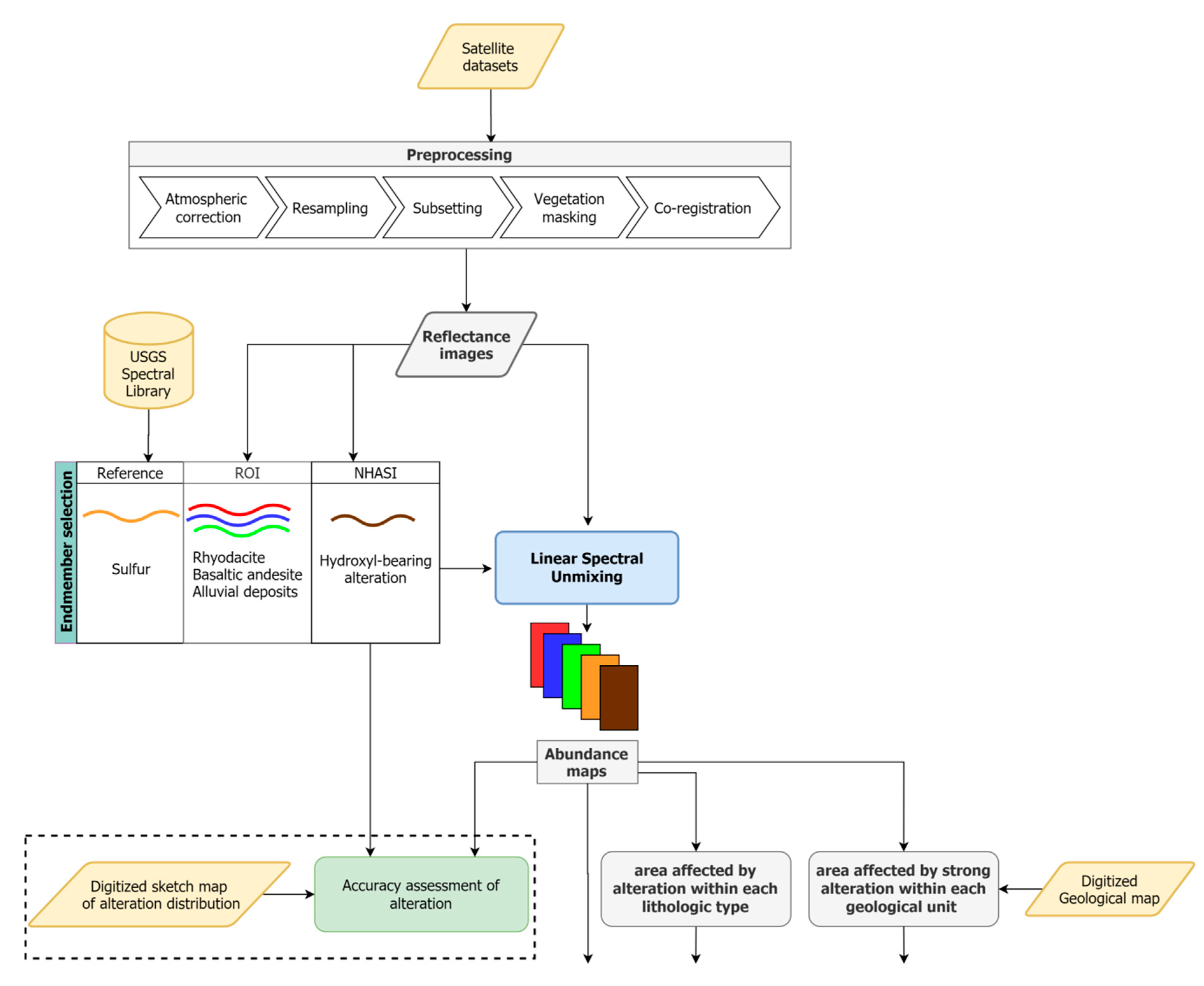
4.1. Preprocessing

The first preprocessing step was to atmospherically correct the datasets. The ASTER L1 and Landsat-8/OLI L1T images were atmospherically corrected using ENVI’s 5.5 FLAASH tool. The Sentinel-2B MSI L1C image was atmospherically corrected using the Sen2Cor processor version 2.8 within ESA’s SNAP software [101], which resulted in 12 spectral bands. All datasets were then resampled to 30-m spatial resolution and spatially subset (Figure 3) to the caldera of Nisyros. Finally, in order to exclude from further processing pixels with dense vegetation, the Normalized Difference Vegetation Index (NDVI) (

Table 1. NDVI formulation for ASTER, Landsat-8/OLI, and Sentinel-2 MSI images expressed in wavelengths.

ASTER [61]	Landsat-8/OLI [61]	Sentinel-2 MSI [61]
$\frac{\left(0.807 \mathsf{\mu }\mathrm{m}-0.661 \mathsf{\mu }\mathrm{m}\right)}{\left(0.807 \mathsf{\mu }\mathrm{m}+0.661 \mathsf{\mu }\mathrm{m}\right)}$	$\frac{\left(0.864 \mathsf{\mu }\mathrm{m}-0.6546 \mathsf{\mu }\mathrm{m}\right)}{\left(0.864 \mathsf{\mu }\mathrm{m}+0.6546 \mathsf{\mu }\mathrm{m}\right)}$	$\frac{\left(0.865 \mathsf{\mu }\mathrm{m}-0.665 \mathsf{\mu }\mathrm{m}\right)}{\left(0.865 \mathsf{\mu }\mathrm{m}+0.665 \mathsf{\mu }\mathrm{m}\right)}$

) was calculated for each one of the three datasets and the respective mask was applied to each one of them in order to retain only pixels with NDVI values less than 0.3 (bare soil to sparse vegetation pixels). Finally, we co-registered the datasets using the ASTER image as reference.

4.2. Main Processing

4.2.1. Endmember Selection

Due to the low dimensionality of the multispectral data, only five endmembers were taken into consideration. Three endmembers represented the main distinctive lithologies in the area, the two primary volcanic lithologies (named hereafter “rhyodacites”, representing acidic to intermediary lava compositions, and “basaltic andesites”, representing basic to intermediary lava compositions) and alluvial/beach deposits (named hereafter “alluvial deposits”). Two endmembers represented the argillic hydrothermal alteration materials (named hereafter “hydroxyl-bearing alteration” and “sulfur”). Scree and other loose materials were not represented by endmembers due to their mixed compositions that included, among others, the two primary volcanic lithologies. Lacustrine deposits and mudflows related to hydrothermal explosions were of mainly clay composition (illite, kaolinite, and montmorillonite) and were represented by the hydroxyl-bearing alteration endmember.

For the endmember selection and extraction, two different approaches were followed: (1) pixel-based endmember selection [102] and (2) retrieval from the USGS spectral library. The pixel-based approach was followed for the retrieval of the four endmembers. More specifically, the endmembers “rhyodacites”, “basaltic andesites”, and “alluvial deposits” were extracted from the images by the use of regions of interest (ROIs). More specifically, first, we identified from the 1:15,000 digitized geological map [68] the areas corresponding to the different lithologies and then, by superimposing them to each dataset, we selected 9x9 ROIs within these areas, so that they were as far as possible from hydrothermal field. The means of the spectral signatures of the pixels within the identified ROIs were then computed and used as the endmembers for the respective lithologies. For the “hydroxyl-bearing alteration”, the endmember was retrieved by calculating the normalized hydrothermal alteration spectral index (NHASI) on each dataset, as shown in

Table 2. The normalized hydrothermal alteration spectral index (NHASI) formulation for ASTER, Landsat-8/OLI, and Sentinel-2 MSI data, expressed in wavelengths.

ASTER [103,104]	Landsat-8/OLI [61]	Sentinel-2 MSI [61]
$\frac{\left(1.656 \mathsf{\mu }\mathrm{m}-2.167 \mathsf{\mu }\mathrm{m}\right)}{\left(1.656 \mathsf{\mu }\mathrm{m}+2.167 \mathsf{\mu }\mathrm{m}\right)}$	$\frac{\left(1.609 \mathsf{\mu }\mathrm{m}-2.201 \mathsf{\mu }\mathrm{m}\right)}{\left(1.609 \mathsf{\mu }\mathrm{m}+2.201 \mathsf{\mu }\mathrm{m}\right)}$	$\frac{\left(1.610 \mathsf{\mu }\mathrm{m}-2.190 \mathsf{\mu }\mathrm{m}\right)}{\left(1.610 \mathsf{\mu }\mathrm{m}+2.190 \mathsf{\mu }\mathrm{m}\right)}$

. The spectral signature of the pixel presenting the highest NHASI value was used as the “hydroxyl-bearing alteration” endmember for each dataset.

Finally, the sulfur endmember was retrieved from the USGS Spectral Library online Version 7 (pure mineral sulfur sample “Sulfur GDS94 Reagent BECKa AREF”), resampled to the spectral bands of each one of the three satellites. Figure 4 shows the plots of the spectral signatures of the endmembers for each multispectral dataset.

4.2.2. Spectral Unmixing

The $n=5$ endmembers were used in the SU process, which was applied separately to each dataset. In this study, we adopted the linear mixing model defined as:

$$\mathit{y}={\sum }_{i=1}^n{a}_i{\mathit{x}}_i$$

(1)

where the spectral signature $\mathit{y}$ of a certain pixel is assumed to be expressed as a linear combination of the spectral signatures of the selected endmembers ${\mathit{x}}_i$s ($a_i$s denotes the respective coefficients). Then, the abundances $a_i$ of the n = 5 endmembers were estimated via the unmixing process, which in our case utilized the least squares error criterion [65,105,106] in its unconstrained form.

Let us discuss briefly the geometrically perspective of the above criterion. The number of bands l specifies the dimensionality of the Euclidean space where the spectral signatures live. The unconstrained unmixing process projects the vector y of the spectral signature of the pixel under consideration to the $n$-dimensional space $S$ spanned by the vectors of the spectral signatures of the selected endmembers ${\mathit{x}}_1,\dots ,{\mathit{x}}_n$ and the abundances are the coefficients of the linear combination of ${\mathit{x}}_1,\dots ,{\mathit{x}}_n$ that defines the projection y′ of y on $S$. Since the abundances are indicative of the correlation of y with the respective ${\mathit{x}}_i$s, a negative abundance is likely to indicate reduced correlation between y and the respective ${\mathit{x}}_i$. From this perspective, we set it equal to zero.

The unconstrained form of SU was selected because, in contrast to constrained SU forms (sum-to-one and/or non-negativity), it resulted in smaller residues than the constrained model.

5. Results

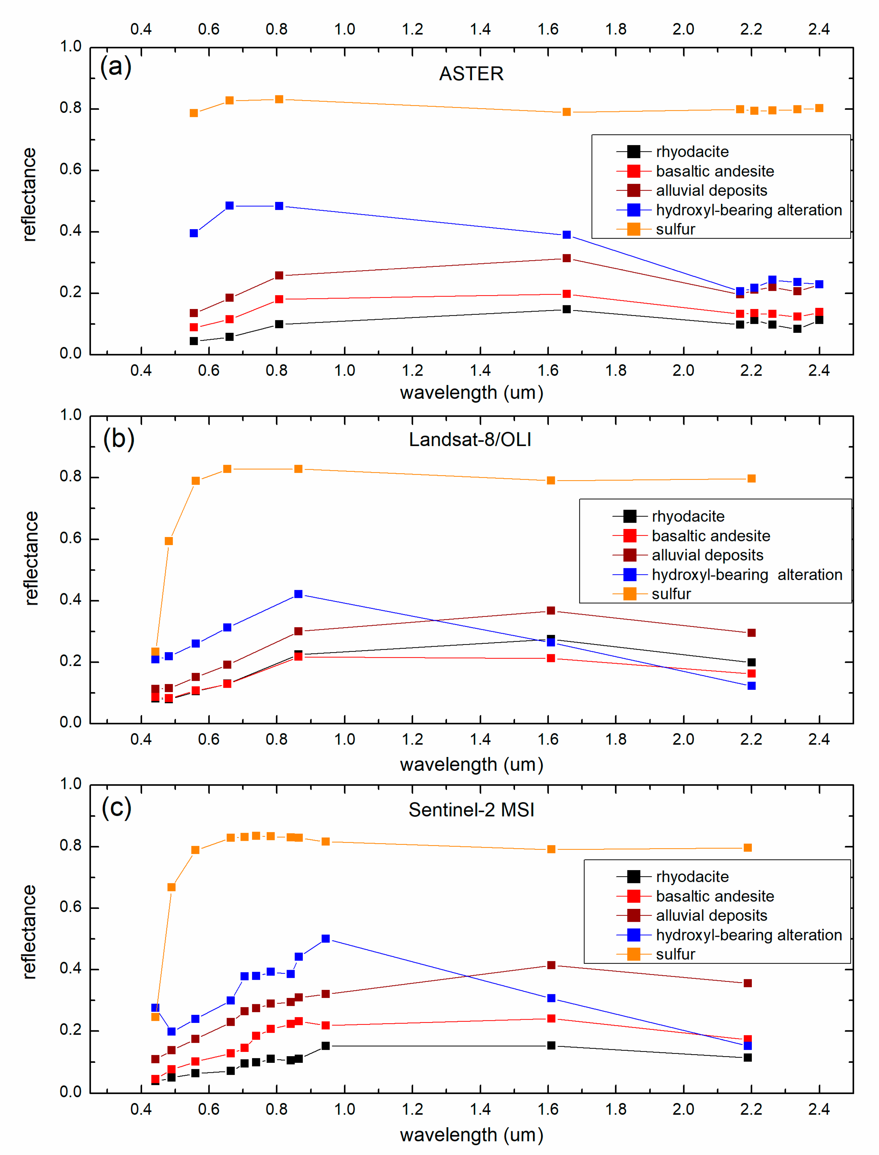
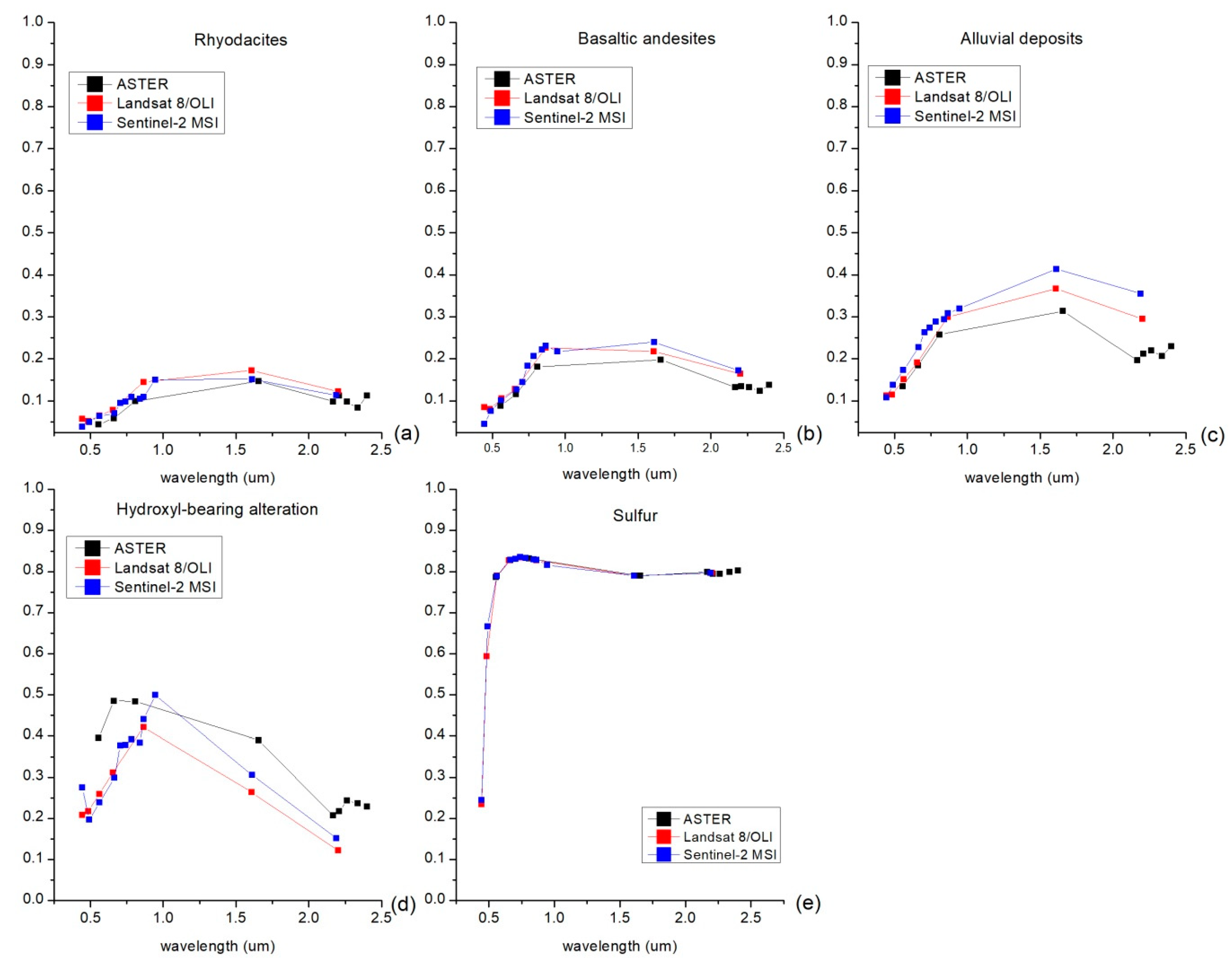
5.1. Endmember Spectra

The spectral signatures of the five endmembers selected for each dataset are presented in Figure 4. The endmembers of the two primary volcanic products (rhyodacites and basaltic andesites) generally showed low reflectances and, in the case of ASTER and Landsat-8/OLI, a similar pattern as well. However, they seemed to better differentiate in the NIR region of Sentinel-2 MSI between 0.7 μm and 1 μm. Compared to them, the alluvial deposits endmembers showed higher reflectances and, in general, the same pattern. They seemed to differentiate in the SWIR bands of ASTER and the NIR bands of Sentinel-2 MSI.

The hydroxyl-bearing alteration endmembers showed higher reflectance values than those of the endmembers of the two primary volcanic products [34] and alluvial deposits. In general, their spectral pattern differed from all other endmembers. Specifically, in ASTER it was differentiated between 0.55–0.8 μm, in Landsat-8/OLI in the SWIR region, and in Sentinel-2 MSI it differed in the whole spectral range. Finally, the sulfur endmember exhibited very high reflectance, compared to the other endmembers. In addition, it exhibited a significantly different pattern from all other endmembers in all three sensors. More specifically, it was featureless for the range of wavelengths between 0.6 μm and 2.4 μm, while it presented a characteristic steep slope between 0.4–0.6 μm. However, the latter was detected only by Landsat-8/OLI and Sentinel-2 MSI, since they had an adequate number of spectral bands in this spectral region.

5.2. Spectral Unmixing Results

The five abundance maps for each sensor (rhyodacites, basaltic andesites, alluvial deposits, hydroxyl-bearing alteration, and sulfur) issued from SU are presented in Figure 5. Its rows correspond to the endmembers and its columns to the sensors.

5.2.1. ASTER

The abundance map of rhyodacites in ASTER showed a broad spatial distribution throughout the whole study area (Figure 5a). The highest abundance values were observed around Lofos Dome, at the central sector craters (Phlegethon, Mikros, and Megalos Polybotes craters), around the Nis-1 and Nis-2 geothermal wells, inside of and at the south-southeastern rim of Stefanos crater and the southern and southeastern part of the study area. On the other hand, basaltic andesites showed high abundances at few specific locations where rhyodacites were present in low abundances (Figure 5d). The highest basaltic andesites abundances appeared only in a few pixels located inside Stefanos crater. A different pattern was observed for the alluvial deposits (Figure 5g). In particular, high abundances of alluvial deposits were observed in the northeastern part of the study area and southwest of Stefanos crater. It is worth noting that in certain areas, such as southwest of Stefanos crater and northeast of the study area at Nis-1 and Nis-2 geothermal wells, both rhyodacites and alluvial deposits appeared in high abundances. Concerning the hydroxyl-bearing alteration, the corresponding abundance map (Figure 5j) showed a distinctive pattern in the central part of the study area, presenting three main centers: (1) Lofos dome and the central sector craters, (2) southeast of and inside Stefanos crater, and (3) the outside rims of Kaminakia craters. There was also a distinctive NE-oriented linear high-abundance pattern west of Stefanos crater that seemed to follow the main NE–SW striking fault system within the caldera. Finally, the spatial distribution of sulfur (Figure 5m) generally followed the hydroxyl-bearing alteration pattern, with few local differentiations such as the inner part of Stefanos crater, Kaminakia craters, and the surrounding areas of the Nis-1 and Nis-2 geothermal wells.

5.2.2. Landsat-8/OLI

The Landsat-8/OLI rhyodacite abundance map (Figure 5b) included few pixels with high abundances northwest of Lofos Dome and north of the hydrothermal area of the central sector craters (Phlegethon, Mikros, and Megalos Polybotes craters) and south-southeast of Stefanos and Kaminakia craters. The spatial distribution of basaltic andesites was very limited and similar to the spatial pattern of rhyodacites (e.g., southeast of the central sector craters), as shown in Figure 5e. On the other hand, the alluvial deposits covered the largest part of the study area (Figure 5h). The highest abundances were observed at Lofos dome, the central sector craters, inside Stefanos crater, and the eastern part of the study area. Hydroxyl-bearing alteration (Figure 5k) showed a similar pattern with alluvial deposits (Figure 5h) and followed the same characteristic three-center pattern that was observed in the ASTER-corresponding result. High abundances were observed at Lofos dome and the related hydrothermal area of the central sector craters (Phlegethon, Mikros, and Megalos Polybotes craters), within Stefanos crater, and at the outer rim of Kaminakia craters. Finally, sulfur high abundances (Figure 5n) were mainly observed within the hydrothermal areas of the central sector craters (Phlegethon, Mikros, and Megalos Polybotes craters), east of and inside Stefanos and the outer rim of Kaminakia craters.

5.2.3. Sentinel-2 MSI

The Sentinel-2 MSI results showed that rhyodacites (Figure 5c) mainly appeared at the periphery of the study area in the form of scattered pixels of intermediate to high abundance. Basaltic andesites (Figure 5f) generally appeared in low abundances, except from few sparse pixels, at Lakki plain, inside Stefanos crater, and in the periphery of the study area. The alluvial deposits (Figure 5i) showed high abundances northeast of the study area around the Nis-1 and Nis-2 geothermal wells and inside Stefanos crater. The pattern of alluvial deposits resembled the corresponding alluvial deposits’ pattern of Landsat-8/OLI image and, in a larger extent, compared with the ASTER corresponding abundance map. Concerning the hydroxyl-bearing alteration (Figure 5l), the same distinctive spatial pattern was observed as in the ASTER and Landsat-8/OLI corresponding maps with the highest abundance values located at Lofos Dome, the central sector craters (Phlegethon, Mikros, and Megalos Polybotes craters), and inside Stefanos crater. Similar to the ASTER and Landsat-8/OLI corresponding results, the sulfur abundance spatial distribution (Figure 5o) generally followed the pattern of the hydroxyl-bearing alteration.

6. Discussion

The assessment of spectral unmixing results was carried out into three directions, namely, in terms of (1) the agreement of the unmixing results with the available geological information, (2) the agreement among the results obtained by the three sensors, and (3) the characteristics of the spatial distribution pattern of the hydrothermal alteration as they were mapped by the three sensors.

Since the assessment was carried out quantitatively, we first computed the following three quantities.

(1)

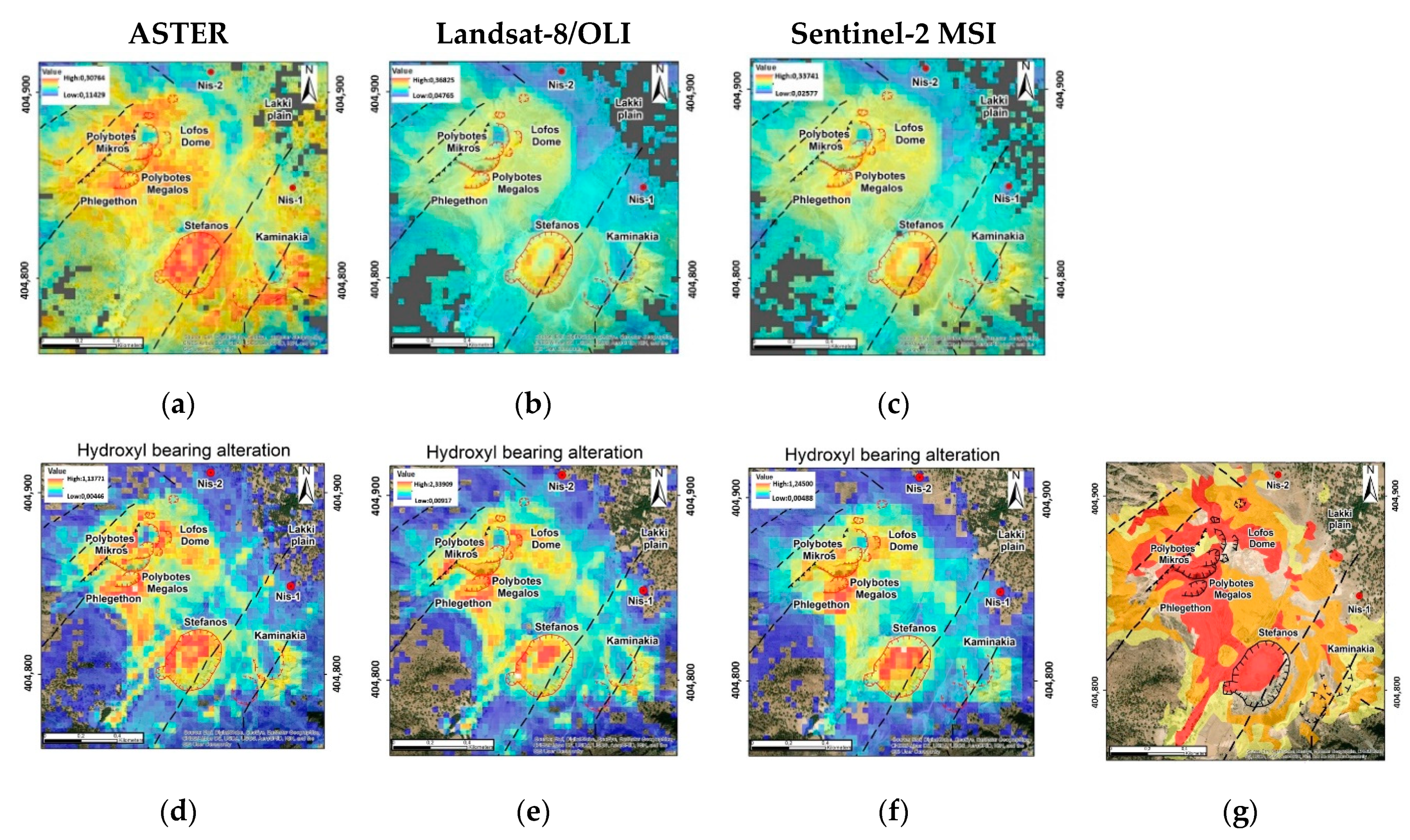
Associating the “low”, “intermediate”, and “high” values of the hydroxyl-bearing alteration abundances with the “weak alteration”, “middle alteration”, and “strong alteration” categories given in the sketch map of the distribution of hydrothermal alteration in the hydrothermal field of the southern Lakki plain shown in [68], respectively, we calculated the confusion matrices and overall accuracies (one for each dataset) concerning NHASI, with respect to the reference map. In the same spirit, we associated the “low”, “intermediate”, and “high” values of the NHASI index with the “weak alteration”, “middle alteration”, and “strong alteration” categories given in the reference map and calculated the respective confusion matrices and overall accuracies. To achieve this, we digitized, georeferenced, and co-registered the sketch map. We then digitized the three different alteration categories and produced a classification map (named hereafter “reference map”) with three classes, namely, “weak”, “medium”, and “strong” alteration, as described by [68]. We then quantized the NHASI and hydroxyl-bearing alteration abundance maps into three groups. Specifically, let $X$ denote a map that may be either an NHASI or a hydroxyl-bearing alteration abundance map. Neglecting the pixels of $X$ where no alteration information is given by the reference map, we divided the range of values of the remaining pixels (which correspond to some degree of alteration) of $X$ into three intervals as follows: Denoting by $n_w, n_m, n_s$ the number of pixels that were characterized as “weak”, “middle”, and “strong” alteration, respectively, in the reference map, the first (leftmost) interval contained the $n_w$ lowest values of $X$, the next (middle) interval contained the next $n_m$ lowest values and, finally, the last (rightmost) contained the $n_s$ highest values of $X$. Actually, this can be seen as a histogram equalization process of $X$, with respect to the reference map. The pixels of $X$ that were in the lower-valued interval were labeled as “low” value pixels, those that were in the second interval were labeled as “intermediate” value pixels, and those that were in the third were labeled as “high” value pixels. Then, we calculated the confusion matrix (CF). In our case, this was a $3x3$ matrix where the rows corresponded to classes “weak” (first row), “middle” (second row), and “strong” (third row) from the reference map and the columns corresponded to the “low” (first column), “intermediate” (second column), and “high” (third column), associated with $X$. The $\left(i,j\right)$ entry of $CF$ equaled the number of pixels that belonged simultaneously to the $i$-th class of the reference map and $j$-th interval of values in $X$. For example, the (1,2) entry of $CF$ contained the pixels that were characterized as “weak” alteration in the reference map and “intermediate” valued in $X$. Based on the $CF$, the overall accuracy was the ratio of the sum of the diagonal elements of $CF$ divided by the total number of pixels (recall that we are referring only to the pixels that were characterized as altered to some degree in the reference map).

Table 3. Confusion matrices between the three alteration degree classes of the reference map (source [68]) (in lines) and the three categories of the quantized NHASI values and hydroxyl-bearing alteration abundances (issued from SU) (in columns). The overall accuracy is also shown in percentage. OA: overall accuracy.

	NHASI Low	NHASI Intermediary	NHASI High	SU Low	SU Intermediary	SU High
ASTER
weak alteration	165	212	69	233	159	44
middle alteration	131	291	195	56	356	188
strong alteration	36	114	182	19	85	204
OA	45.8%			59%
Landsat-8/OLI
weak alteration	204	181	60	206	188	49
middle alteration	91	317	209	47	337	216
strong alteration	18	119	176	17	75	178
OA	50.7%			54.9%
Sentinel-2 MSI
weak alteration	195	181	68	239	162	32
middle alteration	92	317	203	39	368	203
strong alteration	25	114	173	9	80	198
OA	50%			60.5%

contains the $CF$s and the associated overall accuracies (OAs) for all six maps (the NHASI index map and the hydroxyl-bearing alteration SU map, for each one of the three datasets).

(2)

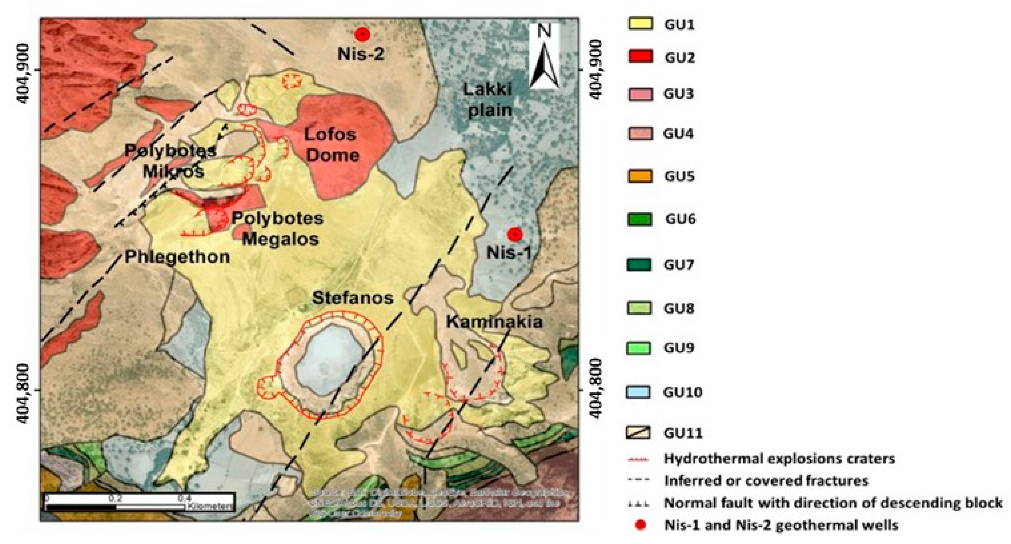
For each endmember, we calculated the percentage of its participation (in terms of number of pixels) within each one of the general lithologic types present in the study area. In order to facilitate the following discussion, we grouped the 11 LSUs present within the study area (described in Section 2) into five general lithologic types, namely, (1) acidic to intermediary lava flows and breccias (LSUs 2, 3, 4, and 5), (2) basic to intermediary lava flows (LSUs 6, 7, 8, and 9), (3) lacustrine and debris flows (LSU1), (4) alluvial/beach deposits (LSU10), and (5) scree deposits (LSU11). Then, for each endmember, we counted the number of pixels with positive abundances within each one of the five aforementioned lithologic types and we computed the corresponding percentage over the total surface. These percentages are presented in

Table 4. Percentage of endmember within each general lithologic type present in the study area.

		Rhyodacite	Basaltic Andesite	Alluvial Deposits	Hydroxyl-Bearing Alteration	Sulfur
		%	%	%	%	%
ASTER
Debris flow/lacustrine deposits		32.3	16.7	30.3	54.5	51.4
Acidic to intermediary lava flows and breccia		11	16.1	9.6	10.3	17.2
Basic to intermediary lava flows		3.3	5.6	0.5	1	0
Alluvial/beach deposits		12.5	23	21.4	7	6.9
Scree deposits		40.9	38.6	38.1	27.2	24.6
	Total	100	100	100	100	100
Landsat-8/OLI
Debris flow/lacustrine deposits		17.9	3.8	39.4	49.9	56.7
Acidic to intermediary lava flows and breccia		8.2	19.1	13.3	12.2	4.6
Basic to intermediary lava flows		4.8	5.4	0.9	0.4	1.5
Alluvial/beach deposits		20.1	24.6	11.3	8.4	13.7
Scree deposits		49	47.1	35.1	29.2	23.5
	Total	100	100	100	100	100
Sentinel-2 MSI
Debris flow/lacustrine deposits		11.7	11.3	36.7	53.5	58.1
Acidic to intermediary lava flows and breccia		11.2	16.5	10.4	12.5	11.1
Basic to intermediary lava flows		4.3	5	1.2	0.2	0.4
Alluvial/beach deposits		25.1	19.5	13.8	7.1	7
Scree deposits		47.7	47.7	38.1	26.6	23.4
	Total	100	100	100	100	100

.

(3)

For each one of the 11 LSUs, we calculated the percentage of surface containing pixels with “high” to “very high” hydroxyl-bearing alteration and sulfur abundance. To this end, we first quantized each of the hydroxyl-bearing alteration and the sulfur abundance maps into four groups. Specifically, we divided the range of values of the pixels of each map into four equally sized intervals and we counted the number of pixels lying in each one of them (according to their abundance value). Those that were in the lower-valued interval (they exhibited low abundance values) were labeled as “low abundance” pixels and those that were in one of the next three intervals were labeled as “intermediate abundance”, “high abundance”, and “very high abundance” pixels. Then, we counted the number of pixels showing high and very high abundance of hydroxyl-bearing alteration and sulfur inside each LSU and we calculated the corresponding percentages over the total number of pixels of each LSU. The results are presented in

Table 5. Percentage of surface affected by high hydroxyl-bearing alteration within each LSU (described in Section 2).

	ASTER		Landsat-8/OLI		Sentinel-2 MSI
LSU	Hydroxyl-Bearing Alteration	Sulfur	Hydroxyl-Bearing Alteration	Sulfur	Hydroxyl-Bearing Alteration	Sulfur
	%	%	%	%	%	%
1	27.0	1.7	21.4	5.9	20.6	7.5
2	23.4	4.7	21.7	0.4	27.2	3.0
3	0	0	0	0	0	0
4	0	0	0	0	0	0
5	0	0	0	0	0	0
6	0	0	0	0	0	0
7	0	0	0	0	0	0
8	0	0	0	0	0	0
9	0	0	0	0	0	0
10	7.0	0.2	4.7	0.5	7.5	2.6
11	8.5	1.3	7.4	0.1	6.7	2.2

.

The discussion is organized in the following four sections that concern: (1) the comparison of the results obtained by SU with those obtained by the use of the alteration SI (NHASI) in terms of accuracy using the reference map, (2) the area of each primary lithology that was affected by the hydrothermal alteration (LSUs as depicted in the geological map and grouped in the aforementioned five lithologic types) as well as the area affected by strong alteration within each specific LSU, (3) the comparison of the results obtained by the three sensors, and (4) various aspects of the proposed processing methodology.

6.1. Comparison between SU and Alteration SI for Mapping Hydrothermal Alteration

In order to reveal the advantage of using the SU method to map hydrothermal alteration over the use of an alteration SI such as NHASI (that detects Al-OH bearing minerals), we compared the two corresponding maps, namely, the hydroxyl-bearing alteration abundance map and the NHASI map, with the reference map (Figure 6g). Although the NHASI maps from the three sensors (Figure 6a–c) captured the general pattern, they did not always successfully depict the different degrees of alteration or the correct spatial extent of the alteration field. This argument is also supported quantitatively through the OAs given in Table 3 (maximum OA ~50%). On the other hand, the corresponding hydroxyl-bearing alteration abundance maps issued from SU (Figure 6d–f) not only successfully mapped the alteration field (maximum OA ~60% in Table 3) but also showed that different abundance values (low, intermediate, and high) seemed to highlight the different degrees of alteration (weak, middle, and strong, respectively). Characteristic examples are the distinctive NE-oriented linear high-alteration abundance pattern west of Stefanos crater that seemed to follow the main NE–SW striking fault system within the caldera and the very characteristic halo that was created by mud and altered rocks, in the inner part of Stefanos crater and in the area of Megalos and Mikros Polybotes from the explosions of 1887. The advantage of SU over NHASI can be explained by the fact that the NHASI approach utilizes scalar information, relating only a few entries of the spectral signature of a pixel, while SU utilizes the entire spectral signature.

Although, SU systematically outperforms NHASI for all three sensors, the most significant differences between the two methods were observed in ASTER and Sentinel-2 MSI with the SU systematically providing the best results, meaning that the different alteration classes of the reference map were best represented by the three hydroxyl-bearing alteration abundance categories.

Focusing now to the more detailed information given by the $CFs$, one can observe that, more or less, all six results exhibited a difficulty in discriminating between the “middle” and the “strong” alteration, as they are defined in the reference map. However, this problem was more serious in the NHASI maps than in the SU maps.

6.2. The Hydrothermal Alteration Field

It is well known that the presence of clays and sulphates, which are argillic alterations, can be indicators of hydrothermally altered rocks in regions of known geothermal activity such the Nisyros caldera. Based on this fact, in this study, clays were represented by the hydroxyl-bearing alteration endmember, which corresponded to the pixel with the highest NHASI value, a well-known SI that takes into account the Al-OH feature at 2.2 μm.

From the results obtained from the application of the proposed methodology on the three multispectral datasets, it was observed that, in general, they all satisfactorily mapped the exposed alteration area of interest, especially ASTER and Sentinel-2. The result demonstrates that mapping alteration using a related hydroxyl-bearing alteration endmember can provide a reliable result (especially for the aforementioned two sensors). The results sufficiently delineated the spatial distribution of the argillic hydrothermal alteration (which encompasses the argillic alteration minerals kaolinite, montmorillonite, illite). Moreover, we were able to calculate the percentage of the total surface per lithology affected by alteration, due to the availability of a relative geological map [68]. In the sequel, we highlight the main locations where each lithology is met and we comment on the associated hydrothermal alteration results provided by the proposed methodology.

(1)

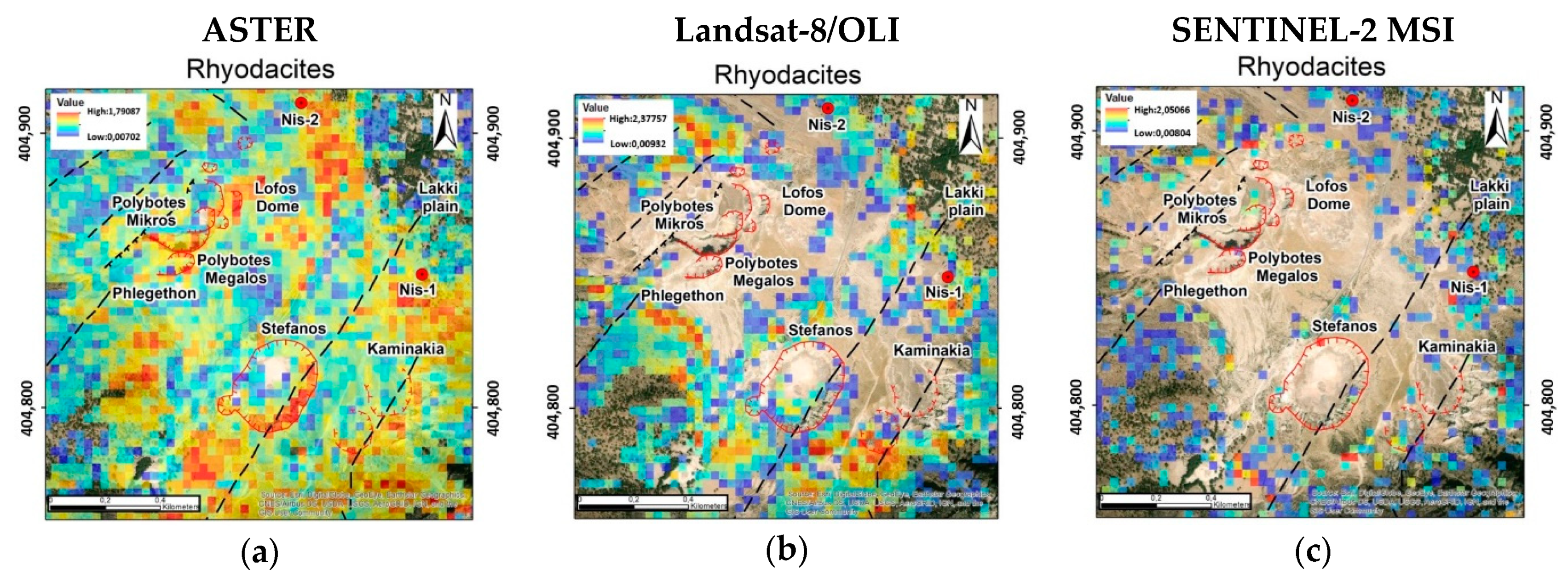
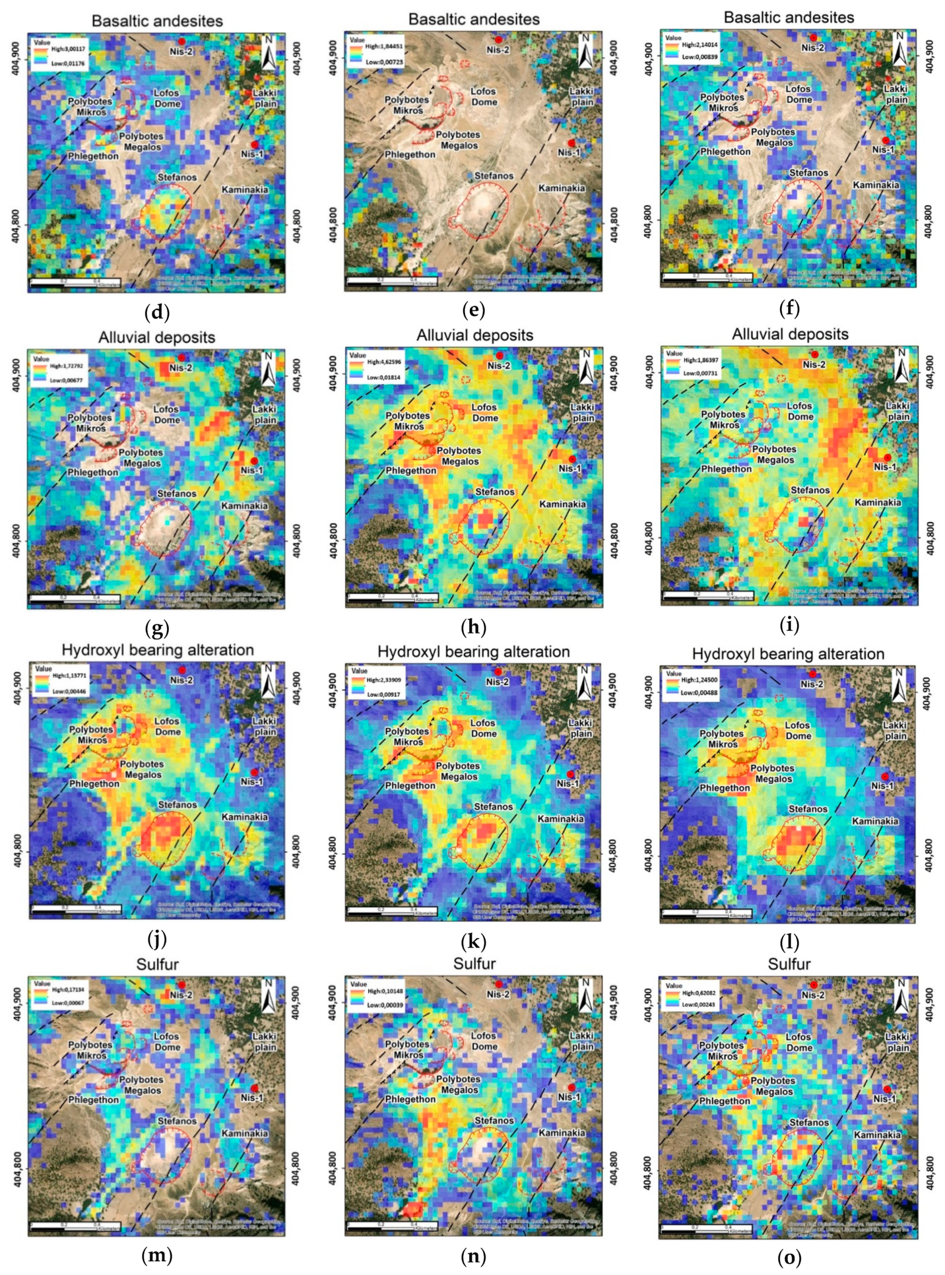
Acidic to intermediary lavas and breccias (LSU2, 3, 4, and 5) are present in Lofos dome, locally at the five central sector hydrothermal craters and the west-northwest part of the study area (Figure 2 in red color). According to the results shown in Table 4, hydrothermal alteration seems to affect 10.3–12.5% of their total surface (Table 4). However, we observed that the only LSU that is partially affected by high to very high alteration (23–27% of the total surface) is LSU2, namely, the rhyodacitic lava domes and lavas of the last volcanic cycle of Post-Caldera Eruptive Cycle located at Lofos Dome and the central sector craters (Table 5). Accordingly, the supplementary sulfur deposits cover only 4.5–17% of the acidic to intermediary lavas’ surface (Table 4) and, as it is the case of hydroxyl-bearing alteration, high to very high sulfur abundances cover a very small surface of only LSU2 outcrops (0.4% to 4.7%) (Table 5). This result is in accordance with the documented severely altered terrains concentrated in the LSU2 zone due to their contact with hydrothermal fluids [68,76]. It is also worth noting here that SU also succeeded in mapping the very characteristic halo that is created by mud and altered rocks in the area of Megalos and Mikros Polybotes from the explosions of 1887 [68].

(2)

Basic to intermediary composition lava outcrops (LSU 6–9): The outcrops of these formations are very limited, located in the southeastern part of the study area (Figure 2 in green color) as well as in the southeastern wall of Stefanos crater. In contrast with acidic to intermediary lavas, basic to intermediary lava compositions show low to intermediate hydrothermal alteration abundances, which cover less than 1% of their total surface (Table 5). A characteristic example is the presence hydroxyl-bearing alteration abundances mapped in the Stefanos crater wall (especially from ASTER data) which are in accordance with [86] where it is referred that the bottom of Stefanos crater consists of fragments of andesitic lavas exposed along the steep inner crater walls. Kaminakia crater is also partly filled by the talus of the caldera wall and by the deposits of Stefanos crater.

(3)

Quaternary deposits: They include volcano-sedimentary alluvial/beach deposits and volcano-sedimentary old and recent scree deposits. In particular:

3.1 

Volcano-Sedimentary Alluvial/Beach Deposits (LSU10)

They are loose materials of Quaternary alluvial/beach deposits constituting a mixture of epiclastic and sandy materials [68]. Hydroxyl-bearing alteration and sulfur deposits cover a relatively small fraction of the LSU10 surface (7–8.4%) (Table 4), while high to very high abundances of hydroxyl-bearing alteration cover 4.5–7.5% of their surface and sulfur deposits 0.2–2.6%, correspondingly (Table 5).

3.2 

Volcano-Sedimentary Old and Recent Scree Deposits (LSU11)

They are denoted in light brown color in Figure 2. They are composed of loose materials that mainly contain primary volcanic products [68]. High to very high hydrothermal alteration abundances cover 6.7–8.5% of the total LSU11 surface but only 0.1–2.2% of the surface is covered by supplementary sulfur deposits (Table 5). Characteristic example of the successful mapping of alteration on scree deposits is the inner part of Stefanos crater where it is referred to as a transition from old and recent scree to more alluvial matrix materials, hydrothermally affected by advanced argillic alteration processes [86].

(4)

Debris flows and lacustrine deposits (LSU1): They are mainly related to historical hydrothermal explosions within the caldera (Figure 2 in yellow color). They belong to the Hydrothermal Explosive Cycle [68] and are directly related to high hydrothermal alteration and sulfur presence. According to [68,76], the main hydrothermal alteration field is located south of Lakki, in the central sector, including Stefanos crater and Kaminakia crater, and at the central sector craters (Mikros, Megalos Polybotes, and Flegethon). All three hydroxyl-bearing alteration abundance maps show similar spatial patterns, which successfully map hydrothermal alteration in LSU1. Specifically, the alteration covers 49.9–54.5% of the total LSU1 surface (Table 4). High to very high alteration abundances are mainly observed in the northwestern part of the area and affect 20.6–27% of the total LSU1 surface (Table 5). Furthermore, the main accompanying product of fumarolic and hydrothermal activity in this sector is the supplementary sulfur. Sulfur is mainly mapped by SU in Stefanos and Kaminakia craters. Indeed, according to [68], there are diffuse fumaroles and mud pools with sulfur deposits at the southeastern floor of Stefanos crater and sulfur cascades from fumaroles at the southeastern part of Kaminakia crater. Sulfur covers an extensive area of the LSU1 surface (51.4–58.1%), presenting high to very high abundance values in 1.7–7.5% of the LSU1 surface.

Resuming the above, the SU results showed that the hydrothermal alteration field (including supplementary sulfur deposits) seems to affect all five general lithologies but to a different degree. Debris flows and lacustrine deposits located in the central area (LSU1) are, as expected, the most affected in terms of total surface and highest abundance coverage. Three other specific lithostratigraphic units are also affected, namely, LSU2, LSU10, and LSU11. Furthermore, hydroxyl-bearing alteration and sulfur show a characteristic spatial pattern, depicted by all three sensors, with three main centers located at Lofos Dome and the central sector craters, Stefanos crater and Kaminakia crater, where the highest alteration abundance values are observed. Additionally, a distinctive NE-oriented linear high-abundance pattern west of Stefanos crater seems to follow the main NE-oriented striking fault system within the caldera.

6.3. Comparison of the Overall SU Results among the Three Sensors

In this subsection, we broaden our focus from the hydroxyl-bearing alteration maps (resulting from the proposed methodology when applied on the three datasets) to the consideration of all the abundance maps produced for each one of the five endmembers that participated in the spectral unmixing. Considering Table 4, it was obvious that the results obtained by the proposed methodology when applied on the three different multispectral datasets did not exhibit significant differences in the sense that the percentage values of each endmember were distributed in a similar way among the five different lithologies (Table 4). Generally, there was a less-than-10% difference in the surface coverage of each endmember per lithology. Few exceptions include basaltic andesite in lacustrine deposits, rhyodacite in lacustrine deposits, and alluvial/beach deposits. This similarity may be attributed to the fact that the general pattern of the spectral signatures of the endmembers (Figure 7) used in this study was the same for all three sensors. From a geometrical point of view, this means that the subspaces defined by the endmember spectral signatures for each sensor were similar.

6.4. Methodology

The correct identification of the most representative endmember spectra as well as their number is undoubtedly the most critical step for a successful SU. Endmember identification is also a challenging procedure in the application of SU when working in natural heterogeneous environments or when using data of low dimensionality. The endmember spectra that are extracted from the same image are much more associated with the specific image features compared to library spectra. In addition, they capture the inherent effects related to the sensor and image acquisition conditions. This is the reason why in this study we adopted this option in order to extract four of the five endmembers.

However, two important practical limitations of the endmember identification process originate from the low spatial resolution (30 m) of the data as well as the limited number of spectral bands, which is generally the case when working with multispectral data. In this study, this problem was evident when attempting to identify “pure” signatures of rhyodacitic lavas, basaltic andesites (of scarce and very localized outcrops), and alluvial/beach deposits. Although the selected signatures were based on the geological map, they were most probably not representative of a single material, but were the spectral products of variable proportions of more than one composition (e.g., basaltic andesites and alluvial/beach deposits) or even different degrees of hydrothermal alteration. It was impossible to find totally pure endmembers in a 30 m pixel size across this particular area, which added a degree of uncertainty on the final SU results. This can be seen on the similarities between the rhyodacite and basaltic andesite endmembers extracted from the ASTER and Landsat-8/OLI images (Figure 4a,b). However, this difficulty did not seem to have a significant influence on the SU results.

Another general important issue in SU is the discriminability of endmembers, which depends on the spectral characteristics of the dataset, such as the number and position of the spectral bands in the electromagnetic spectrum. In the present case, there was the example of the spectral signatures of the two lava endmembers in the ASTER image, which showed a similar pattern but they were well distinguished by Sentinel-2 MSI due to Sentinel’s larger number of spectral bands in the VNIR region of the spectrum (Figure 4a,c). The same applies to the case of the spectral signatures of the alluvial deposits, lavas, and the hydrothermal alteration products.

An additional common confounding factor of the SU approach is within-class spectral variability especially when working with low-dimensionality data. This is why, in this study, we addressed this issue by selecting the average spectral signature of a 9 × 9 ROIs for the three primary lithology endmembers. Although this approach alleviates statistical fluctuations (up to some degree) in the specification of an endmember, there is still a degree of uncertainty in the unmixing results.

An additional difficulty we faced in this study was the quantitative evaluation of the results. To the best of our knowledge, the only reference information about the study area was the sketch map provided in [68]. Thus, in order to perform quantitative evaluation of the results, we proceeded to the digitization, georeferencing, co-registration and creation of a classification map of it. Although the resulting map was not an ideal one (due to the errors inserted during the previous processes such as the lack of reference points), it was the only way to implement quantitative evaluations. Of course, due to the previous issues, the obtained results ($CF$s and $OA$s) were useful only for the comparison of the alteration indices’ maps with the SU maps, in terms of a common reference.

Despite the above issues associated with endmember selection, within the present study area, the use of endmembers selected as described in Section 4.2.1 provided a satisfactory result, as shown in the quantitative assessments in Table 3.

It is also worth pointing out a general comment for the spectral unmixing process. Specifically, in several cases the use of the spectral unmixing poses a restriction to the number of the endmembers that can participate in the unmixing process. Speaking rigorously, this number should be less than the number of bands (dimension of the spectral signatures), while, in practice, this number should be significantly less than the number of bands (in our case the number of the endmembers (five) was smaller than the number of bands in each of the three sensors). This restriction can become less severe for hyperspectral datasets, where the number of the bands is significantly greater than the corresponding one in the multispectral data.

7. Conclusions

The aim of this work was to develop a methodology to map a hydrothermal field in a volcanic environment, by applying spectral unmixing on multispectral data from the ASTER, the Landsat-8/OLI, and the Sentinel-2 MSI sensors. The case study was the hydrothermal field in the volcanic environment of Nisyros. The unmixing results obtained by ASTER and Sentinel-2 MSI were better than those of Landsat-8/OLI. However, Landsat-8/OLI also followed the general alteration pattern (as was given in a sketch map in literature that was used as reference), however, at a lower degree of accuracy. This behavior may be attributed to the fact that the general pattern of the spectral signatures of each material endmembers used in this study was similar for all three sensors.

The main challenges faced in this study were the spatial resolution and the complexity of the composition of the existing formations. Despite these difficulties, the proposed methodology successfully mapped the hydrothermal alteration field (in reference to the produced classification map issued from the only existing sketch map of the distribution of hydrothermal alteration in the hydrothermal field of the southern Lakki plain in order to perform quantitative assessments). In addition, a new finding was revealed, namely, the fact that abundances can highlight different degrees of alteration better than conventional methods such as the use of spectral indices, especially in the case of ASTER and Sentinel-2 MSI.

Concerning the hydrothermal field of Nisyros caldera, our findings showed that mainly acidic to intermediary lavas and breccias are affected by alteration. Among these lavas, strong alteration affects only the rhyodacitic lava domes and lavas of the last volcanic cycle of Post-Caldera Eruptive Cycle located at Lofos Dome and the central sector craters. On the other hand, while only a relatively small fraction of the surface of the Quaternary deposits seems to be affected by hydrothermal alteration, the other main lithologies affected by the hydrothermal alteration, both in terms of affected area and intensity of the alteration, were the debris flows and lacustrine deposits at the center of the caldera. These formations are mainly related to the historical hydrothermal explosions and belong to the Hydrothermal Explosive Cycle. In addition, our results are in agreement with previous studies according to which the hydrothermal field of Nisyros caldera presents a characteristic spatial pattern with three main centers of strong alteration located at Lofos Dome and the central sector craters, Stefanos crater and Kaminakia crater.

Future investigations include the use of other spectral unmixing methods, both supervised (where the endmembers are predefined) and unsupervised (where both endmembers and abundances are estimated simultaneously), the investigation of the distribution of alteration-related minerals and the full exploitation of the spectral information (e.g., thermal bands) of the datasets.

References

- Van der Werff, H.M.A.; van der Meer, F.D. Sentinel-2 for mapping iron absorption feature parameters. Remote Sens. 2015, 7, 12635–12653. [Google Scholar] [CrossRef] [Green Version]
- Ge, W.; Cheng, Q.; Tang, Y.; Jing, L.; Gao, C. Lithological classification using Sentinel-2A data in the Shibanjing ophiolite complex in Inner Mongolia, China. Remote Sens. 2018, 10, 638. [Google Scholar] [CrossRef] [Green Version]
- Ge, W.; Cheng, Q.; Jing, L.; Armenakis, C.; Ding, H. Lithological discrimination using ASTER and Sentinel-2A in the Shibanjing ophiolite complex of Beishan orogenic in Inner Mongolia, China. Adv. Space Res. 2018, 62, 1702–1716. [Google Scholar] [CrossRef]
- Hu, B.; Xu, Y.; Wan, B.; Wu, X.; Yi, G. Hydrothermally altered mineral mapping using synthetic application of Sentinel-2A MSI, ASTER and Hyperion data in the Duolong area, Tibetan. Ore Geol. Rev. 2018, 101, 384–397. [Google Scholar] [CrossRef]
- Vasuki, Y.; Yu, L.; Holden, E.; Kovesi, P.; Wedge, D.; Grigg, A.H. The spatial-temporal patterns of land cover changes due to mining activities in the Darling Range, Western Australia: A Visual Analytics Approach. Ore Geol. Rev. 2019, 108, 23–32. [Google Scholar] [CrossRef]
- Pour, A.B.; Hashim, M.; Hong, J.K.; Park, Y. Lithological and alteration mineral mapping in poorly exposed lithologies using Landsat-8 and ASTER satellite data: North-eastern Graham Land, Antarctic Peninsula. Ore Geol. Rev. 2019, 108, 112–133. [Google Scholar] [CrossRef]
- Guha, A.; Vinod Kumar, K. Comparative analysis on utilisation of linear spectral unmixing and band ratio methods for processing ASTER data to delineate bauxite over a part of Chotonagpur plateau, Jharkhand, India. Geocarto Int. 2016, 31, 367–384. [Google Scholar] [CrossRef]
- Hosseinjani, M.; Tangestani, M.H. Mapping alteration minerals using sub-pixel unmixing of ASTER data in the Sarduiyeh area, SE Kerman, Iran. Int. J. Digit. Earth 2011, 4, 487–504. [Google Scholar] [CrossRef]
- Abubakar, A.J.A.; Hashim, M.; Pour, A.B. Identification of hydrothermal alteration minerals associated with geothermal system using ASTER and Hyperion satellite data: A case study from Yankari Park, NE Nigeria. Geocarto Int. 2019, 34, 597–625. [Google Scholar] [CrossRef]
- Pour, A.B.; Park, Y.; Crispini, L.; Läufer, A.; Hong, J.K.; Park, T.Y.S.; Zoheir, B.; Pradhan, B.; Muslim, A.M.; Hossain, M.S.; et al. Mapping listvenite occurrences in the damage zones of Northern Victoria Land, Antarctica using ASTER Satellite Remote Sensing Data. Remote Sens. 2019, 11, 1408. [Google Scholar] [CrossRef] [Green Version]
- Pour, A.B.; Hashim, M.; Park, Y.; Hong, J.K. Mapping alteration mineral zones and lithological units in Antarctic regions using spectral bands of ASTER remote sensing data. Geocarto Int. 2018, 33, 1281–1306. [Google Scholar] [CrossRef]
- Pour, A.B.; Park, T.Y.S.; Park, Y.; Hong, J.K.; Muslim, A.M.; Läufer, A.; Crispini, L.; Pradhan, B.; Zoheir, B.; Rahmani, O.; et al. Landsat-8, Advanced Spaceborne Thermal Emission and Reflection Radiometer, and WorldView-3 Multispectral Satellite Imagery for Prospecting Copper-Gold Mineralization in the Northeastern Inglefield Mobile Belt (IMB), Northwest Greenland. Remote Sens. 2019, 11, 2430. [Google Scholar] [CrossRef] [Green Version]
- Nielsen, A.A. Spectral mixture analysis: Linear and semi-parametric full and iterated partial unmixing in multi-and hyperspectral image data. J. Math. Imaging Vis. 2001, 15, 17–37. [Google Scholar] [CrossRef] [Green Version]
- Pour, A.B.; Hashim, M. Hydrothermal alteration mapping from Landsat-8 data, Sar Cheshmeh copper mining district, south-eastern Islamic Republic of Iran. J. Taibah Univ. Sci. 2015, 9, 155–166. [Google Scholar] [CrossRef]
- Han, T.; Nelson, J. Mapping hydrothermally altered rocks with Landsat 8 imagery: A case study in the KSM and Snowfield zones, northwestern British Columbia. Br. Columbia Geol. Surv. Pap. 2015, 1, 103–112. [Google Scholar]
- Yokoya, N.; Chan, J.C.W.; Segl, K. Potential of resolution-enhanced hyperspectral data for mineral mapping using simulated EnMAP and Sentinel-2 images. Remote Sens. 2016, 8, 172. [Google Scholar] [CrossRef] [Green Version]
- Mezned, N.; Bouzidi, W.; Dkhala, B.; Abdeljaouad, S. Cascade sub-pixel unmixing of aster SWIR data for mapping alteration minerals in tamra sidi-driss SITE, NW Tunisia. In Proceedings of the 2017 IEEE International Geoscience and Remote Sensing Symposium (IGARSS), Fort Worth, TX, USA, 23–28 July 2017; pp. 6267–6270. [Google Scholar] [CrossRef]
- Brandmeier, M. Remote sensing of Carhuarazo volcanic complex using ASTER imagery in Southern Peru to detect alteration zones and volcanic structures—A combined approach of image processing in ENVI and ArcGIS/ArcScene. Geocarto Int. 2010, 25, 629–648. [Google Scholar] [CrossRef]
- Hewson, R.D.; Cudahy, T.J.; Huntington, J.F. Geologic and alteration mapping at Mt fitton, South Australia, using ASTER satellite-borne data. Int. Geosci. Remote Sens. Symp. 2001, 2, 724–726. [Google Scholar] [CrossRef]
- Pour, A.B.; Hashim, M. Identifying areas of high economic-potential copper mineralization using ASTER data in the Urumieh-Dokhtar Volcanic Belt, Iran. Adv. Space Res. 2012, 49, 753–769. [Google Scholar] [CrossRef]
- Ayoobi, I.; Tangestani, M.H. Evaluating the effect of spatial subsetting on subpixel unmixing methodology applied to ASTER over a hydrothermally altered terrain. Int. J. Appl. Earth Obs. Geoinf. 2017, 62, 1–7. [Google Scholar] [CrossRef]
- Abubakar, A.J.; Hashim, M.; Pour, A.B. Spectral mineral mapping for characterization of subtle geothermal prospects using ASTER data. J. Phys. Conf. Ser. 2017, 852. [Google Scholar] [CrossRef] [Green Version]
- Pour, A.B.; Hashim, M.; Marghany, M. Using spectral mapping techniques on short wave infrared bands of ASTER remote sensing data for alteration mineral mapping in SE Iran. Int. J. Phys. Sci. 2011, 6, 917–929. [Google Scholar] [CrossRef]
- Pour, A.B.; Hashim, M. The application of ASTER remote sensing data to porphyry copper and epithermal gold deposits. Ore Geol. Rev. 2012, 44, 1–9. [Google Scholar] [CrossRef] [Green Version]
- Yang, M.; Ren, G.; Han, L.; Yi, H.; Gao, T. Detection of Pb–Zn mineralization zones in west Kunlun using Landsat 8 and ASTER remote sensing data. J. Appl. Remote Sens. 2018, 12, 026018. [Google Scholar] [CrossRef]
- Schwartz, G.M. Hydrothermal alteration. Econ. Geol. 1959, 54, 161–183. [Google Scholar] [CrossRef]
- Meller, C.; Kohl, T. The significance of hydrothermal alteration zones for the mechanical behavior of ageothermal reservoir. Geotherm. Energy 2014, 2, 12. [Google Scholar] [CrossRef] [Green Version]
- Pirajno, F. Hydrothermal Processes and Mineral Systems; Springer Science & Business Media: Berlin, Germany, 2008. [Google Scholar]
- Van der Meer, F.D.; van der Werff, H.M.A.; van Ruitenbeek, F.J.A.; Hecker, C.A.; Bakker, W.H.; Noomen, M.F.; Meijde, M.; Carranza, E.J.M.; Smeth, J.B.; Woldai, T. Multi-and hyperspectral geologic remote sensing: A review. Int. J. Appl. Earth Obs. Geoinf. 2012, 14, 112–128. [Google Scholar] [CrossRef]
- Wang, Q.; Blackburn, G.A.; Onojeghuo, A.O.; Dash, J.; Zhou, L.; Zhang, Y.; Atkinson, P.M. Fusion of Landsat 8 OLI and Sentinel-2 MSI data. IEEE Trans. Geosci. Remote Sens. 2017, 55, 3885–3899. [Google Scholar] [CrossRef] [Green Version]
- Mielke, C.; Boesche, N.K.; Rogass, C.; Kaufmann, H.; Gauert, C.; De Wit, M. Spaceborne mine waste mineralogy monitoring in South Africa, applications for modern push-broom missions: Hyperion/OLI and EnMAP/Sentinel-2. Remote Sens. 2014, 6, 6790–6816. [Google Scholar] [CrossRef] [Green Version]
- Rajendran, S. Characterization of ASTER spectral bands for mapping alteration zones of volcanic massive sulphide deposits. Ore Geol. Rev. 2017, 88, 317–335. [Google Scholar] [CrossRef]
- Noori, L.; Pour, A.B.; Askari, G.; Taghipour, N.; Pradhan, B.; Lee, C.W.; Honarmand, M. Comparison of Different Algorithms to Map Hydrothermal Alteration Zones Using ASTER Remote Sensing Data for Polymetallic Vein-Type Ore Exploration: Toroud–Chahshirin Magmatic Belt (TCMB), North Iran. Remote Sens. 2019, 11, 495. [Google Scholar] [CrossRef] [Green Version]
- Sabins, F.F. Remote sensing for mineral exploration. Ore Geol. Rev. 1999, 14, 157–183. [Google Scholar] [CrossRef]
- Tangestani, M.H.; Moore, F. Iron oxide and hydroxyl enhancement using the Crosta Method: A case study from the Zagros Belt, Fars Province, Iran. Int. J. Appl. Earth Obs. Geoinf. 2000, 2, 140–146. [Google Scholar] [CrossRef]
- Goward, S.N.; Masek, J.G.; Williams, D.L.; Irons, J.R.; Thompson, R.J. The Landsat 7 mission Terrestrial research and applications for the 21st century. Remote Sens. Environ. 2001, 78, 3–12. [Google Scholar] [CrossRef]
- Gabr, S.; Ghulam, A.; Kusky, T. Detecting areas of high-potential gold mineralization using ASTER data. Ore Geol. Rev. 2010, 38, 59–69. [Google Scholar] [CrossRef]
- Mars, J.C.; Rowan, L.C. Spectral assessment of new ASTER SWIR surface reflectance data products for spectroscopic mapping of rocks and minerals. Remote Sens. Environ. 2010, 114, 2011–2025. [Google Scholar] [CrossRef]
- Mia, B.; Fujimitsu, Y. Mapping hydrothermal altered mineral deposits using Landsat 7 ETM+ image in and around Kuju volcano, Kyushu, Japan. J. Earth Syst. Sci. 2012, 121, 1049–1057. [Google Scholar] [CrossRef] [Green Version]
- Liu, L.; Zhou, J.; Han, L.; Xu, X. Mineral mapping and ore prospecting using Landsat TM and Hyperion data, Wushitala, Xinjiang, northwestern China. Ore Geol. Rev. 2017, 81, 280–295. [Google Scholar] [CrossRef]
- Rajendran, S.; Nasir, S. ASTER capability in mapping of mineral resources of arid region: A review on mapping of mineral resources of the Sultanate of Oman. Ore Geol. Rev. 2019, 108, 33–53. [Google Scholar] [CrossRef]
- Mielke, C.; Bösche, N.K.; Rogass, C.; Segl, K.; Gauert, C.; Kaufmann, H. Potential applications of the Sentinel-2 multispectral sensor and the EnMap hyperspectral sensor in mineral exploration. Earsel Eproceedings 2014, 13, 93–102. [Google Scholar] [CrossRef]
- El Kati, I.; Nakhcha, C.; El Bakhchouch, O.; Tabyaoui, H. Application of Aster and Sentinel-2A Images for geological mapping in arid regions: The Safsafate Area in the Neogen Guercif basin, Northern Morocco. Int. J. Adv. Remote Sens. GIS 2018, 7, 2782–2792. [Google Scholar] [CrossRef]
- Ducart, D.F.; Crósta, A.P.; Filho, C.R.S.; Coniglio, J. Alteration mineralogy at the Cerro La Mina epithermal prospect, Patagonia, Argentina: Field mapping, short-wave infrared spectroscopy, and ASTER images. Econ. Geol. 2006, 101, 981–996. [Google Scholar] [CrossRef]
- Zhang, X.; Pazner, M. Comparison of lithologic mapping with ASTER, Hyperion, and ETM data in the southeastern Chocolate Mountains, USA. Photogramm. Eng. Remote Sens. 2007, 73, 555–561. [Google Scholar] [CrossRef]
- Tangestani, M.H.; Jaffari, L.; Vincent, R.K.; Sridhar, B.M. Spectral characterization and ASTER-based lithological mapping of an ophiolite complex: A case study from Neyriz ophiolite, SW Iran. Remote Sens. Environ. 2011, 115, 2243–2254. [Google Scholar] [CrossRef]
- Amer, R.; Kusky, T.; El Mezayen, A. Remote sensing detection of gold related alteration zones in Um Rus area, Central Eastern Desert of Egypt. Adv. Space Res. 2012, 49, 121–134. [Google Scholar] [CrossRef]
- Mas, J.F.; Flores, J.J. The application of artificial neural networks to the analysis of remotely sensed data. Int. J. Remote Sens. 2008, 29, 617–663. [Google Scholar] [CrossRef]
- Duro, D.C.; Franklin, S.E.; Dubé, M.G. A comparison of pixel-based and object-based image analysis with selected machine learning algorithms for the classification of agricultural landscapes using SPOT-5 HRG imagery. Remote Sens. Environ. 2012, 118, 259–272. [Google Scholar] [CrossRef]
- Khatami, R.; Mountrakis, G.; Stehman, S.V. A meta-analysis of remote sensing research on supervised pixel-based land-cover image classification processes: General guidelines for practitioners and future research. Remote Sens. Environ. 2016, 177, 89–100. [Google Scholar] [CrossRef] [Green Version]
- Tompolidi, A.; Sykioti, O.; Koutroumbas, K.; Parcharidis, I. Mapping hydrothermal altered areas within the caldera of Nisyros volcano using clustering on multispectral data of ASTER and Sentinel-2. In Proceedings of the 2nd Workshop of Remote Sensing and Space Applications in Geosciences and Geohazards, Athens, Greece, 26 February 2020. [Google Scholar]
- Tompolidi, A.; Sykioti, O.; Koutroumbas, K.; Parcharidis, I. Detection of hydrothermal alteration on volcanic environments applying clustering on Landsat 8 OLI data. Case study: The Nisyros caldera (Greece). In Proceedings of the Conference HGS 2019: 12th International Conference of the Hellenic Geographical Society, Athens, Greece, 1–4 November 2019. [Google Scholar] [CrossRef]
- Tompolidi, A.; Sykioti, O.; Koutroumbas, K.; Xenaki, S.; Parcharidis, I. Potential of Sentinel-2 data on detecting hydrothermal alteration using clustering: The case of Nisyros caldera (Greece). In Proceedings of the Conference GSG 2019: 15th International Congress of the Geological Society of Greece, Athens, Greece, 22–24 May 2019; p. 766. [Google Scholar]
- Podwysocki, M.H.; Segal, D.B.; Abrams, M.J. Use of multispectral scanner images for assessment of hydrothermal alteration in the Marysvale, Utah, mining area. Econ. Geol. 1983, 78, 675–687. [Google Scholar] [CrossRef]
- Jackson, R.D. Spectral indices in n-space. Remote Sens. Environ. 1983, 13, 409–421. [Google Scholar] [CrossRef]
- Philipson, W.; Teng, W. Operational interpretation of AVHRR vegetation indices for world crop information. Photogramm. Eng. Remote Sens. 1988, 54, 55–59. [Google Scholar]
- Sabins, F.F. Remote Sensing Principles and Interpretation, 3rd ed.; W.H. Freeman: New York, NY, USA, 1997; p. 494. [Google Scholar]
- Knepper, D.H. Mapping hydrothermal alteration with Landsat thematic mapper data. In Remote Sensing in Exploration Geology: Golden, Colorado to Washington; Wiley Online Library: Hoboken, NJ, USA, 1989; Volume 1, pp. 13–21. [Google Scholar] [CrossRef]
- Eiswerth, B.; Rowan, L. Analyses of Landsat thematic mapper images of study areas located in western Bolivia, northern Chile, and southern Peru. In Investigationes de Metales Preciosos en le Complejo Volcanico Neogeno-Cuaternario de los Andes Centrales (Investigations on Precious Metals in the Neogene-Quaternary Volcanic Complex of the Central Andes); Servicio Geológico Boliviano-Servicio Nacional de Geología y Minería, Chile-Instituto Geológico Minero y Metalúrgico, Perú-United States Geological Survey. Banco Interamericano de Desarollo: Washington, DC, USA, 1993; Volume 5, pp. 17–44. [Google Scholar]
- Kaufmann, H. Mineral exploration along the Aqaba-Levant Structure by use of TM-data. Concepts, processing and results. Int. J. Remote Sens. (Print) 1988, 9, 1639–1658. [Google Scholar] [CrossRef]
- Van der Werff., H.; van der Meer, F. Sentinel-2A MSI and Landsat 8 OLI provide data continuity for geological remote sensing. Remote Sens. 2016, 8, 883. [Google Scholar] [CrossRef] [Green Version]
- Van der Meer, F.D.; van der Werff, H.M.A.; van Ruitenbeek, F.J.A. Potential of ESA’s Sentinel-2 for geological applications. Remote Sens. Environ. 2014, 148, 124–133. [Google Scholar] [CrossRef]
- Pour, A.B.; Hashim, M. Application of advanced spaceborne thermal emission and reflection radiometer (ASTER) data in geological mapping. Int. J. Phys. Sci. 2011, 6, 7657–7668. [Google Scholar] [CrossRef]
- Keshava, N. A survey of spectral unmixing algorithms. Linc. Lab. J. 2003, 14, 55–78. [Google Scholar]
- Quintano, C.; Fernández-Manso, A.; Shimabukuro, Y.E.; Pereira, G. Spectral unmixing. Int. J. Remote Sens. 2012, 33, 5307–5340. [Google Scholar] [CrossRef]
- Khaleghi, M.; Ranjbar, H.; Abedini, A.; Calagari, A.A. Synergetic use of the Sentinel-2, ASTER, and Landsat-8 data for hydrothermal alteration and iron oxide minerals mapping in a mine scale. Acta Geodyn. Geromater. 2020, 17, 311–329. [Google Scholar] [CrossRef]
- Rajan Girija, R.; Mayappan, S. Mapping of mineral resources and lithological units: A review of remote sensing techniques. Int. J. Image Data Fusion. 2019, 10, 79–106. [Google Scholar] [CrossRef]
- Dietrich, V.J.; Lagios, E. Nisyros Volcano: The Kos-Yali-Nisyros Volcanic Field; Springer: Berlin/Heidelberg, Germany, 2017. [Google Scholar]
- Papanikolaou, D.; Lekkas, E.L.; Sakelariou, D. Volcanic stratigraphy and evolution of the Nisyros volcano. Bull. Geol. Soc. Greece 1991, 25, 405–419. [Google Scholar]
- Tibaldi, A.; Pasquare, F.A.; Papanikolaou, D.; Nomikou, P. Tectonics of Nisyros Island, Greece, by field and offshore data, and analogue modelling. J. Struct. Geol. 2008, 30, 1489–1506. [Google Scholar] [CrossRef]
- Di Paola, G.M. Volcanology and petrology of Nisyros island (Dodecanese, Greece). Bull. Volcanol. 1974, 38, 944–987. [Google Scholar] [CrossRef]
- Volentik, A.C.M.; Principe, C.; Vanderkluysen, L.; Hunziker, J.C. Stratigraphy of Nisyros volcano (Greece). In The Geology, Geochemistry and Evolution of Nisyros Volcano (Greece), Implications for the Volcanic Hazards. Memoires de Geologie; Hunziker, J.C., Marini, L., Eds.; Section des Sciences de la Terre, Université de Lausanne: Lausanne, Switzerland, 2005; Volume 44, pp. 26–67. [Google Scholar]
- Geotermica Italiana. Nisyros 1 geothermal well. Unpublished PPC-EEC report. 1983; p. 106. [Google Scholar]
- Geotermica Italiana. Nisyros 2 geothermal well. Unpublished PPC-EEC report. 1984; p. 44. [Google Scholar]
- Francalanci, L.; Vougioukalakis, G.E.; Perini, G.; Manetti, P. A West-East Traverse along the magmatism of the south Aegean volcanic arc in the light of volcanological, chemical and isotope data. Dev. Volcanol. 2005, 7, 65–111. [Google Scholar] [CrossRef]
- GEOWARN-IST 12310. Geological Map of Greece, 1:10.000. Geo-Spatial Warning Systems Nisyros Volcano (Greece): An Emergency Case Study. Information Society Technologies Programme. Available online: www.geowarn.ethz.ch (accessed on 16 December 2020).
- Vougioukalakis, G.E. Sheet Nisyros, Geological Map of Greece, 1:25.000; IGME (Institute of Geology and Mineral Exploration): Athens, Greece, 2003. [Google Scholar]
- Vougioukalakis, G.E. Mapping 1987–1988; IGME (Institute of Geology and Mineral Exploration): Athens, Greece, 1993. [Google Scholar]
- Papanikolaou, D.; Lekkas, E.L.; Sakellariou, D. Geological structure and evolution of the Nisyros volcano. In Proceedings of the Congress of the Geological Society of Greece, Athens, Greece, 24 May 1990; Volume 25, pp. 405–419. [Google Scholar]
- Dietrich, V.J. Geology of Nisyros Volcano (Geological mapping (2000–2003, 2010–2015)). In Nisyros Volcano: The Kos-Nisyros Volcanic Field; Springer: Berlin/Heidelberg, Germany, 2017; pp. 57–102. [Google Scholar] [CrossRef]
- Ambrosio, M.; Doveri, M.; Fagioli, M.T.; Marini, L.; Principe, C.; Raco, B. Water–rock interaction in the magmatic-hydrothermal system of Nisyros Island (Greece). J. Volcanol Geother. Res. 2010, 192, 57–68. [Google Scholar] [CrossRef]
- Gorceix, M.H. Sur l’état du volcan de Nisyros au mois de mars 1873. C. R. Seances Acad. Sci. Paris 1873, 77, 597–601. [Google Scholar]
- Gorceix, M.H. Sur la récente éruption de Nisyros. C. R. Seances Acad. Sci. 1873, 77, 1039. [Google Scholar]
- Gorceix, M.H. Sur l’éruption boueuse de Nisyros. C. R. Seances Acad. Sci. 1873, 77, 1474–1477. [Google Scholar]
- Gorceix, M.H. Etude des fumerolles de Nisyros et de quelques-uns des produits des éruptions dont cette ile a été le siège en 1872 et 1873. Ann. Chim. Phys. Paris 1874, 333–354. [Google Scholar]
- Marini, L.; Principe, C.; Chiodini, G.; Cioni, R.; Fytikas, M.; Marinelli, G. Hydrothermal eruptions of Nisyros (Dodecanese, Greece). Past events and present hazard. J. Volcanol. Geother. Res. 1993, 56, 71–94. [Google Scholar] [CrossRef]
- Vougioukalakis, G. Volcanic stratigraphy and evolution of Nisyros island. Bull. Geol. Soc. Greece 1993, 28, 239–258. [Google Scholar]
- Stiros, S.C. Fault pattern of Nisyros Island volcano (Aegean Sea, Greece): Structural, coastal and archaeological evidence. Geol. Soc. Lond. Spec. Publ. 2000, 171, 385–397. [Google Scholar] [CrossRef]
- Nomikou, P. Geodynamic of Dodecanese Islands: Kos and Nisyros Volcanic Field. Ph.D. Thesis, Department of Geology, University of Athens, Athens, Greece, 2004. [Google Scholar]
- Volentik, A.; Vanderkluysen, L.; Principe, C.; Hunziker, J.C. The role of tectonic and volcano-tectonic activity at Nisyros Volcano (Greece). Implic. Volcan. Hazards Mem. Geol. 2005, 44, 67–78. [Google Scholar]
- Lagios, E.; Sakkas, V.; Parcharidis, I.; Dietrich, V. Ground deformation of Nisyros Volcano (Greece) for the period 1995–2002: Results from DInSAR and DGPS observations. Bull. Volcanol. 2005, 68, 201–214. [Google Scholar] [CrossRef]
- Sykioti, O.; Kontoes, C.C.; Elias, P.; Briole, P.; Sachpazi, M.; Paradissis, D.; Kotsis, I. Ground deformation at Nisyros volcano (Greece) detected by ERS-2 SAR differential interferometry. Int. J. Remote Sens. 2003, 24, 183–188. [Google Scholar] [CrossRef]
- Venturi, S.; Tassi, F.; Vaselli, O.; Vougioukalakis, G.E.; Rashed, H.; Kanellopoulos, C.; Caponi, C.; Capecchiacci, F.; Cabassi, J.; Ricci, A.; et al. Active hydrothermal fluids circulation triggering small-scale collapse events: The case of the 2001–2002 fissure in the Lakki Plain (Nisyros Island, Aegean Sea, Greece). Nat. Hazards 2018, 93, 601–626. [Google Scholar] [CrossRef]
- Yamaguchi, Y.; Kahle, A.B.; Tsu, H.; Kawakami, T.; Pniel, M. Overview of advanced spaceborne thermal emission and reflection radiometer (ASTER). IEEE Trans. Geosci. Remote Sens. 1998, 36, 1062–1071. [Google Scholar] [CrossRef] [Green Version]
- Fujisada, H.; Sakuma, F.; Ono, A.; Kudoh, M. Design and preflight performance of ASTER instrument proto flight model. IEEE Trans. Geosci. Remote Sens. 1998, 36, 1152–1160. [Google Scholar] [CrossRef]
- Fujisada, H. Design and performance of ASTER instrument. In Proceedings of the SPIE Proceedings, Advanced Next Generation Satellites, Paris, France, 15 December 1995; Volume 2583, pp. 16–25. [Google Scholar] [CrossRef]
- Roy, D.P.; Wulder, M.A.; Loveland, T.R.; Woodcock, C.E.; Allen, R.G.; Anderson, M.C.; Helder, D.; Irons, J.R.; Johnson, D.M.; Kennedy, R.; et al. Landsat-8: Science and product vision for terrestrial global change research. Remote Sens. Environ. 2014, 145, 154–172. [Google Scholar] [CrossRef] [Green Version]
- US Geological Survey. Landsat 8 (L8) Data User Handbook; Version 0.2; US Geological Survey: EROS Sioux Falls, SD, USA, 29 March 2016.
- Zheng, H.; Du, P.; Chen, J.; Xia, J.; Li, E.; Xu, Z.; Li, X.; Yokoya, N. Performance evaluation of downscaling Sentinel-2 imagery for land use and land cover classification by spectral-spatial features. Remote Sens. 2017, 9, 1274. [Google Scholar] [CrossRef] [Green Version]
- Drusch, M.; Del Bello, U.; Carlier, S.; Colin, O.; Fernandez, V.; Gascon, F.; Hoersch, B.; Isola, C.; Laberinti, P.; Martimort, P. Sentinel-2: ESA’s optical high-resolution mission for GMES operational services. Remote Sens. Environ. 2012, 120, 25–36. [Google Scholar] [CrossRef]
- European Space Agency. Level-2A Prototype Processor for Atmospheric Terrain and Cirrus Correction of Top-of-Atmosphere Level 1C Input Data. Available online: http://step.esa.int/main/third-party-plugins-2/sen2cor/ (accessed on 28 September 2016).
- Kokaly, R.F.; Clark, R.N.; Swayze, G.A.; Livo, K.E.; Hoefen, T.M.; Pearson, N.C.; Wise, R.A.; Benzel, W.M.; Lowers, H.A.; Driscoll, R.L.; et al. USGS Spectral Library Version 7: U.S. Geological Survey Data Series 1035; USGS: Reston, VA, USA, 2017; p. 61. [CrossRef]
- Kalinowski, A.; Oliver, S. ASTER Mineral Index Processing Manual; Technical Report; Geoscience Australia: Canberra, Australia, 2004.
- Henrich, V.; Krauss, G.; Götze, C.; Sandow, C. IDB—Entwicklung EINER Datenbank für Fernerkundungs Indizes. 2012. Available online: http://www.indexdatabase.de (accessed on 10 January 2020).
- Shimabukuro, Y.E.; Smith, J.A. The least-squares mixing models to generate fraction images derived from remote sensing multispectral data. IEEE Trans. Geosci. Remote Sens. 1991, 29, 16–20. [Google Scholar] [CrossRef]
- Settle, J.J.; Drake, N.A. Linear mixing and the estimation of ground cover proportions. Int. J. Remote Sens. 1993, 14, 1159–1177. [Google Scholar] [CrossRef]