H-YOLO: A Single-Shot Ship Detection Approach Based on Region of Interest Preselected Network


 , and
, and
Abstract
:1. Introduction
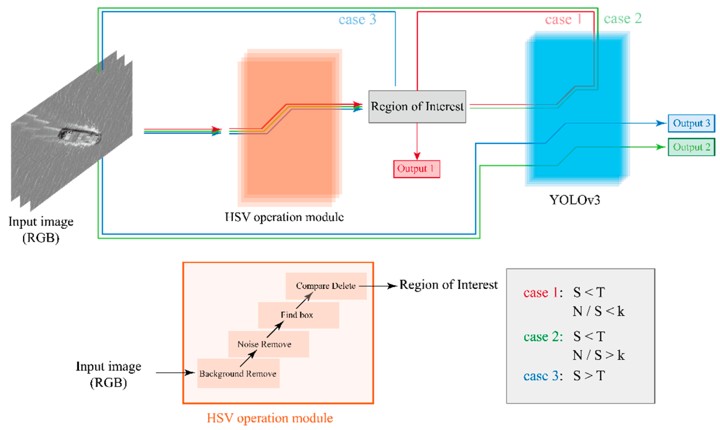
- We introduce a novel vessel remote sensing image classification network, the so-called HSV-YOLO network, consisting of two essential components: an HSV-operation module and a one-stage detection module. To the best of our knowledge, it is the first time that the difference of HSV color space is used as a filter to extract the useful RoIs to reduce detection calculation time.
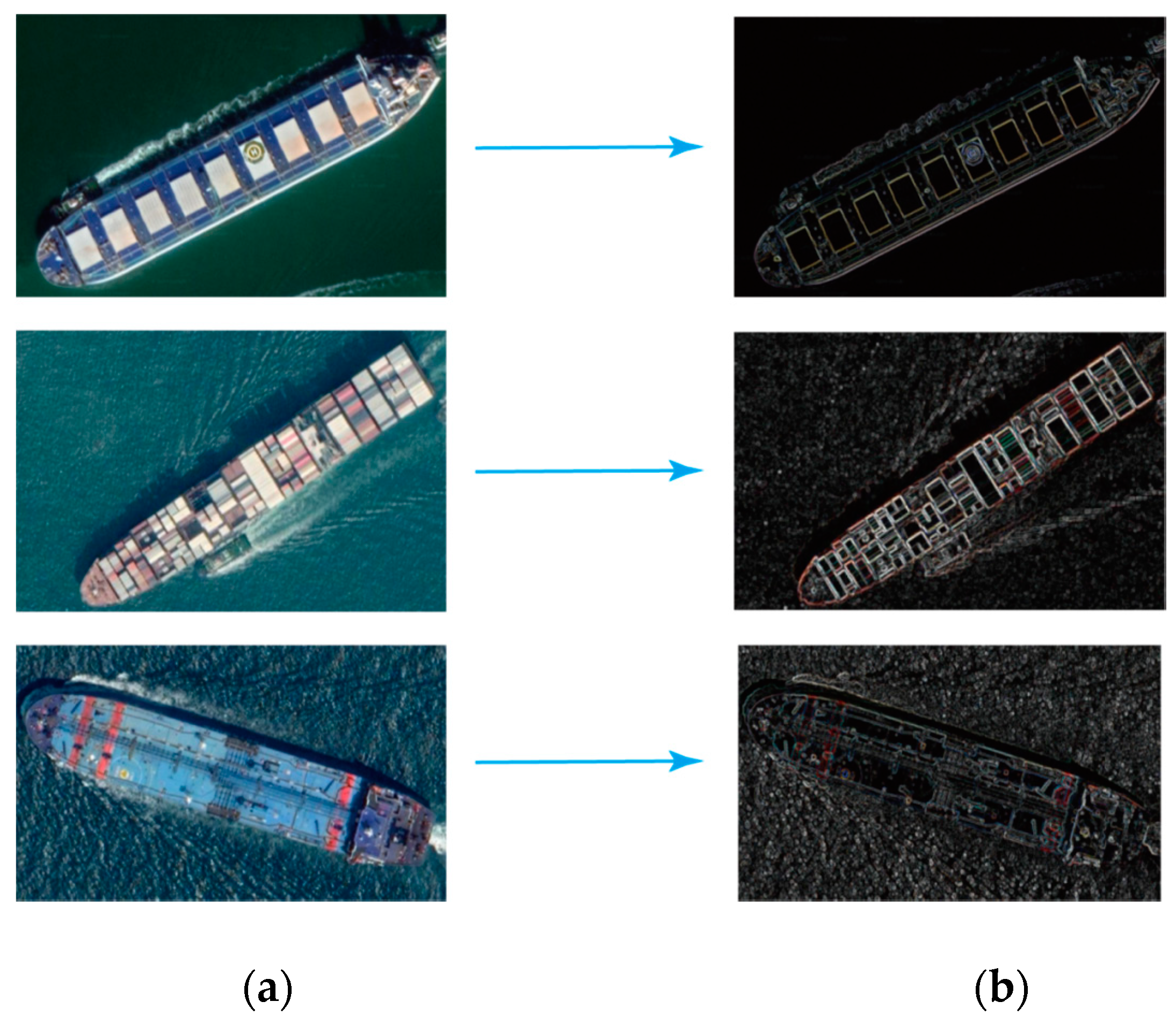
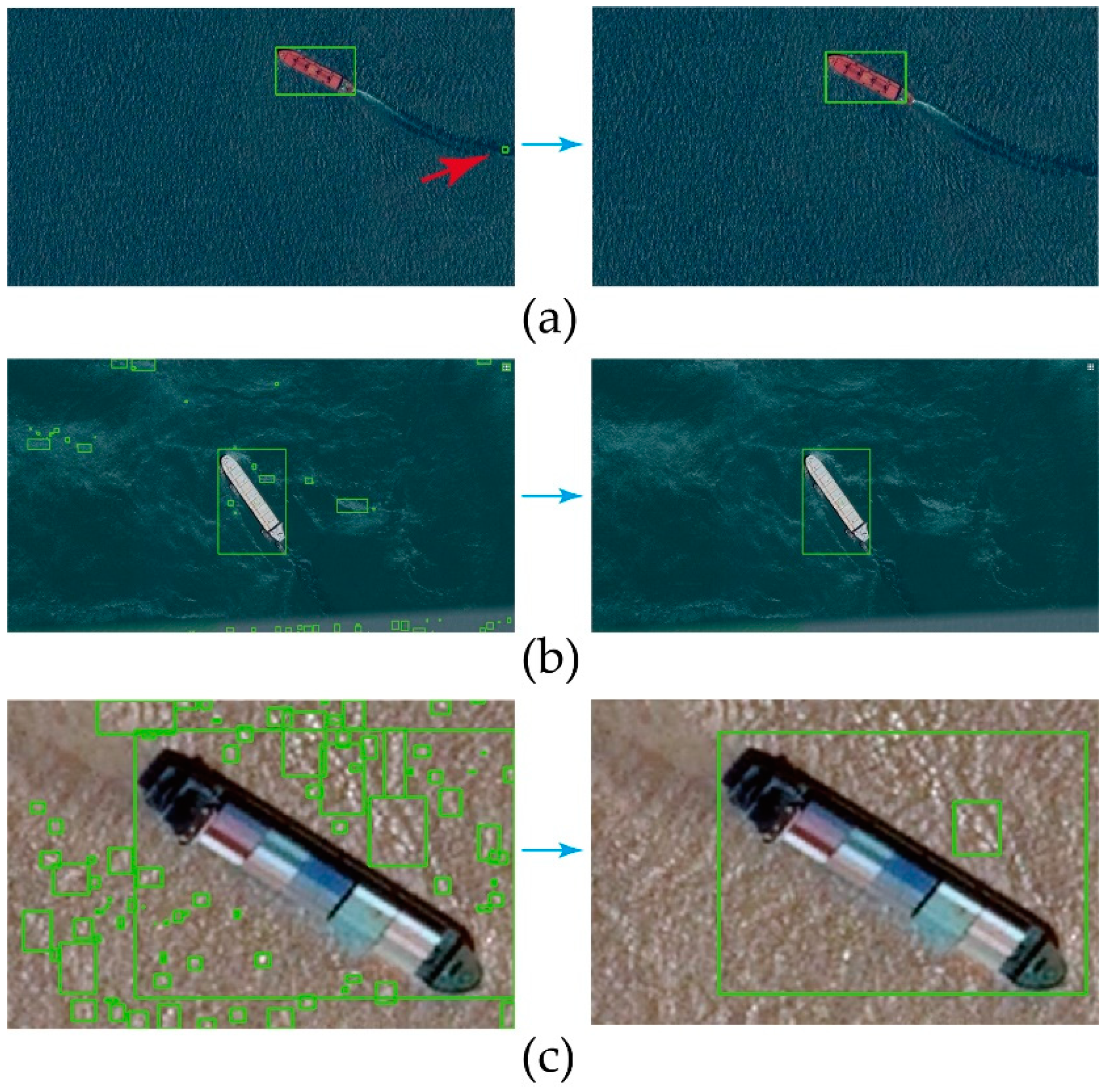
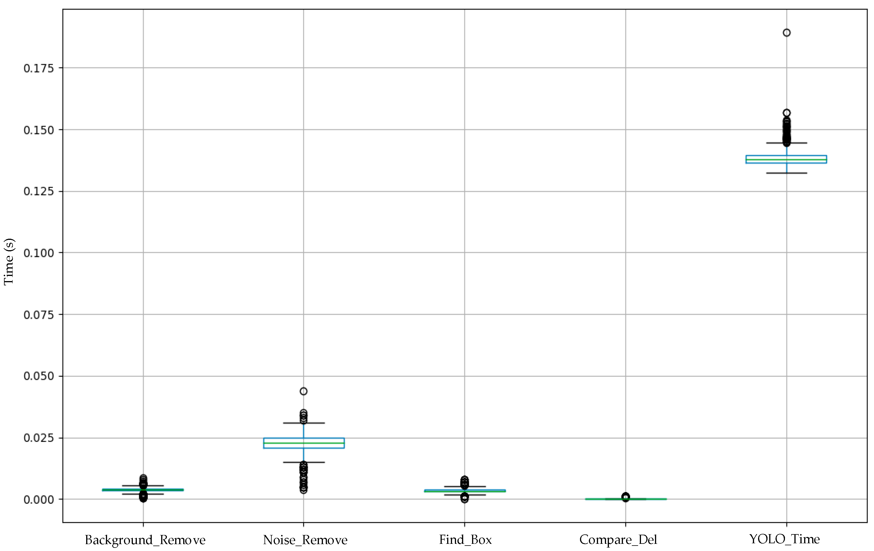
- We designed an HSV-module, which consists of four crucial cores: a background removal operation, a noise removal operation, a box-finding operation, and a noise deletion operation. After these four steps, one can obtain valuable RoIs instead of noisy RoIs, and this in reasonable computing time.
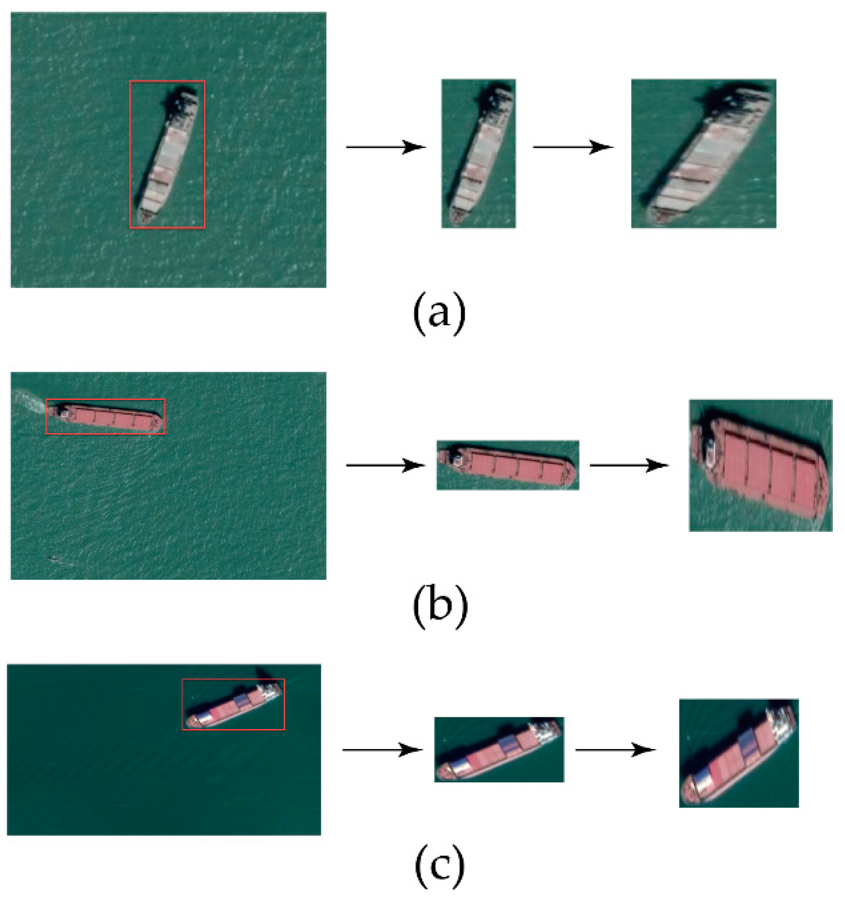
- We designed a pipeline to deal with the outcomes of the HSV-operation module, containing three common situations when processing the images.
2. Material and Method
2.1. HSV-YOLOv3
| Algorithm 1 Case Switching Procedure in H-YOLO |
| Initialize Set total number of identified region of interest S > 0, upper limit T, number of unidentified regions of interest N, and switching value of k; |
| Input: Testing Image Itest; |
| Output: Coordinatei (xi, yi, wi, hi), Labeli; |
| 1: SoR = HSV_Operation(Itest); |
| 2: if SoR > T then |
| 3: Coordinatei, Labeli = Case3(Itest) |
| 4: else |
| 5: if N/S < k then |
| 6: Coordinatei, Labeli = Case1(Itest) |
| 7: else |
| 8: Coordinatei, Labeli = Case2(Itest) |
| 9: end |
| 10: end |
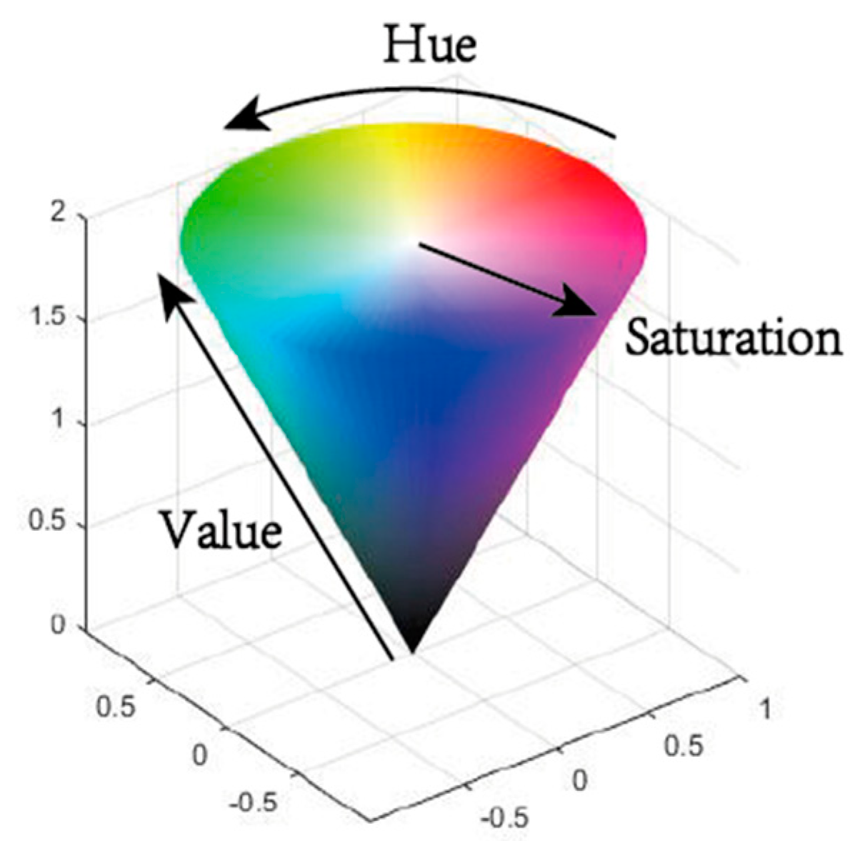
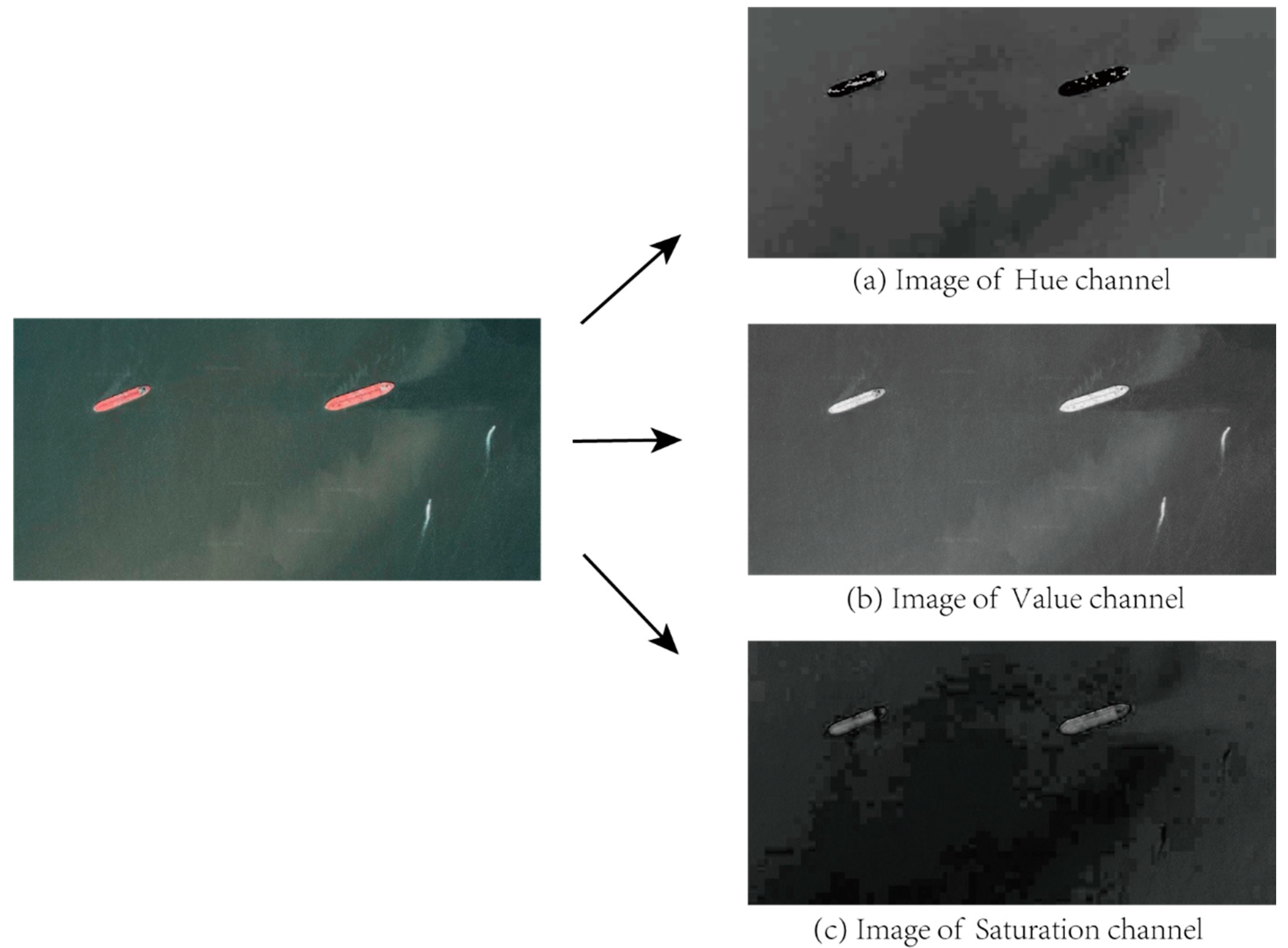
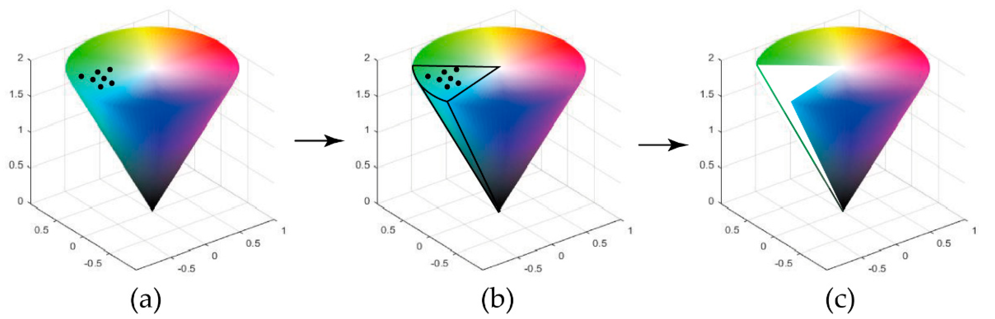
2.2. HSV Processing
2.3. HSV Operation Module
2.3.1. Modeling Approach
2.3.2. Adoptive RoI Extraction
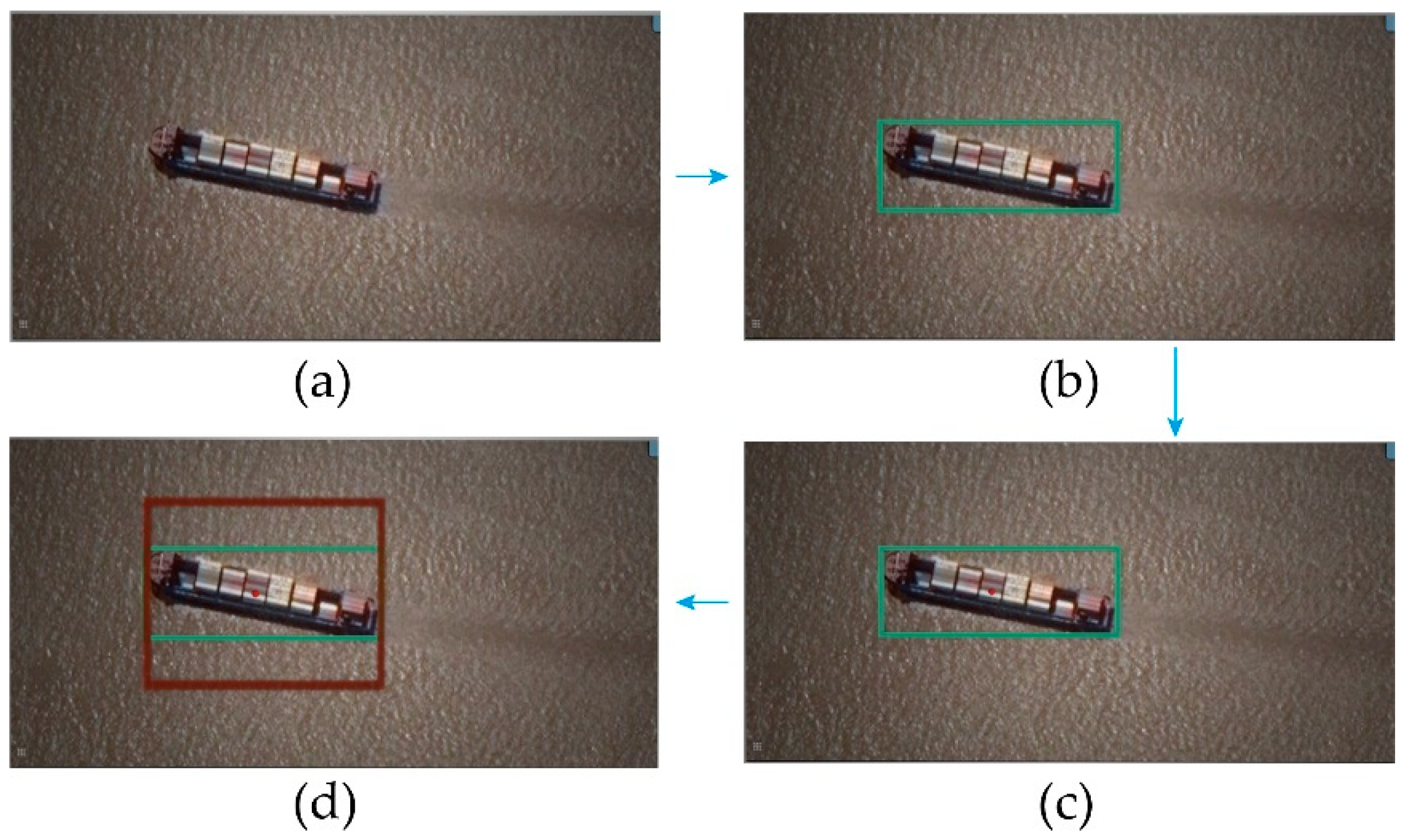
2.3.3. Reference Correction
2.3.4. Anti-Distortion Operation
2.4. Switch Network Conditions
- Switching condition 1: Record the total number of RoIs extracted, based on the HSV difference as S and set an upper limit value as T. When S is more massive than T, it directly jumps out of the extraction process.
- Switching condition 2: Record the unknown number of the input image as N. Set a proportional value as k, and when the N/S ratio exceeds k, the network will be automatically switched to the yolov-3 network.
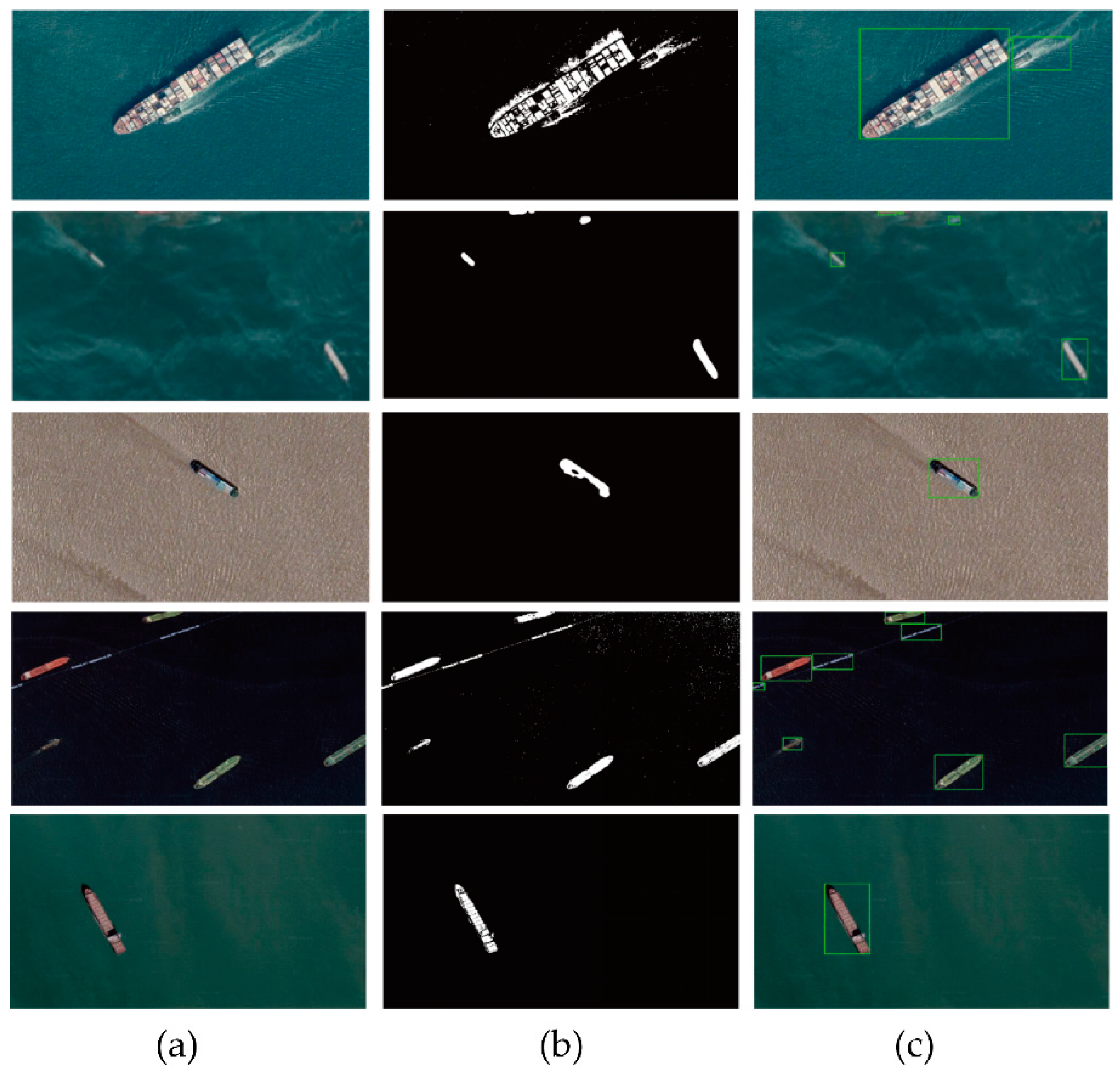
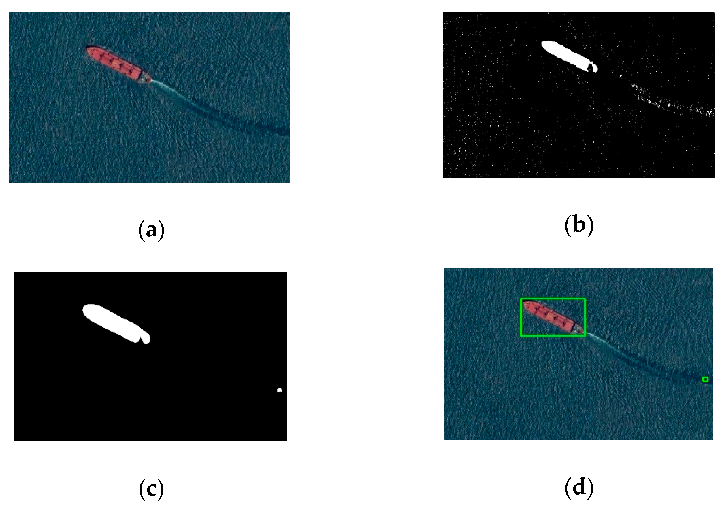
3. Results and Discussion
3.1. Ablation Experiment
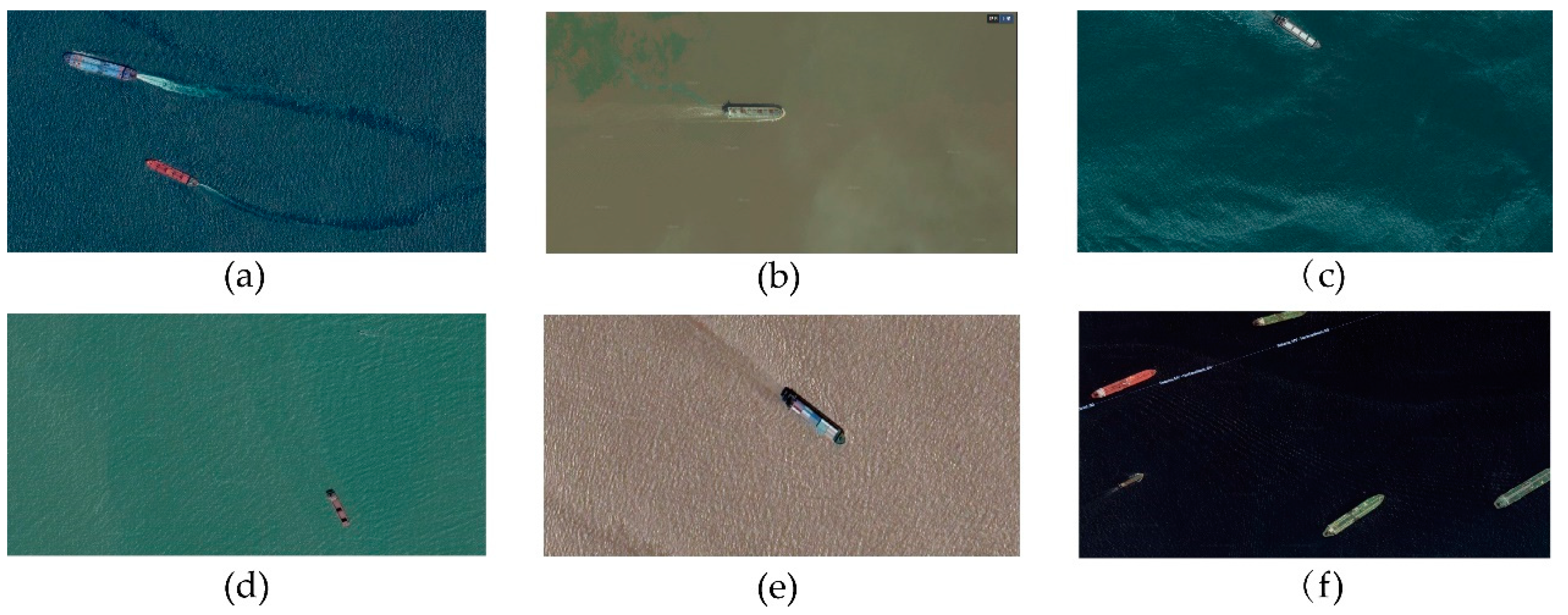
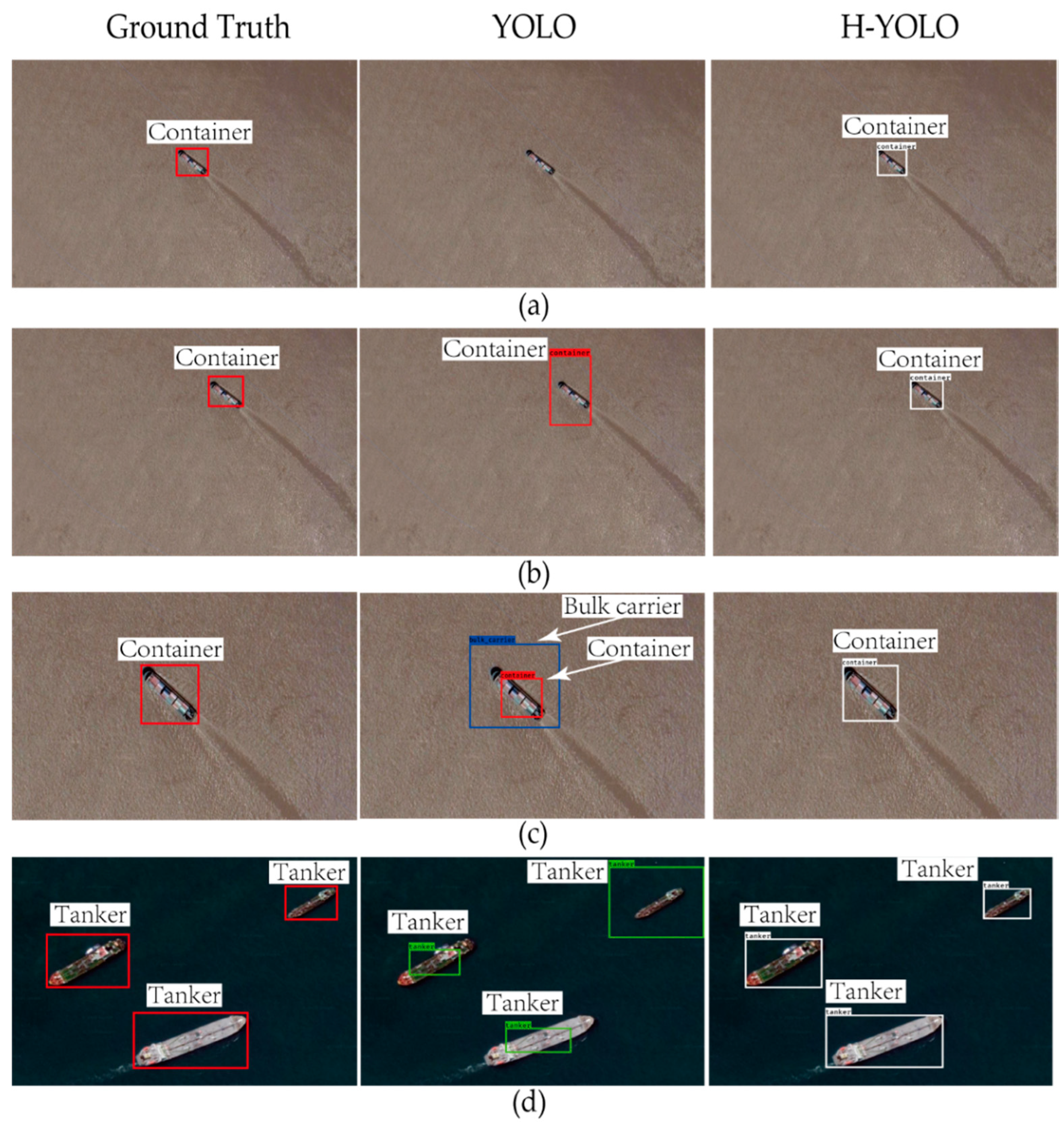
- The training and testing sets are collected from Google Earth, with 560 samples containing categories of tanks, bulk carriers, and containers. Use this small training set to train and test the YOLO-tiny and HSV-base-YOLO-tiny algorithm.
- Use a small sample (including 500 training samples) training set to train the network on the YOLO-tiny framework to get a weight file. YOLOv3-tiny and the improved SV-based-YOLOv3-tiny use the same weight file for testing.
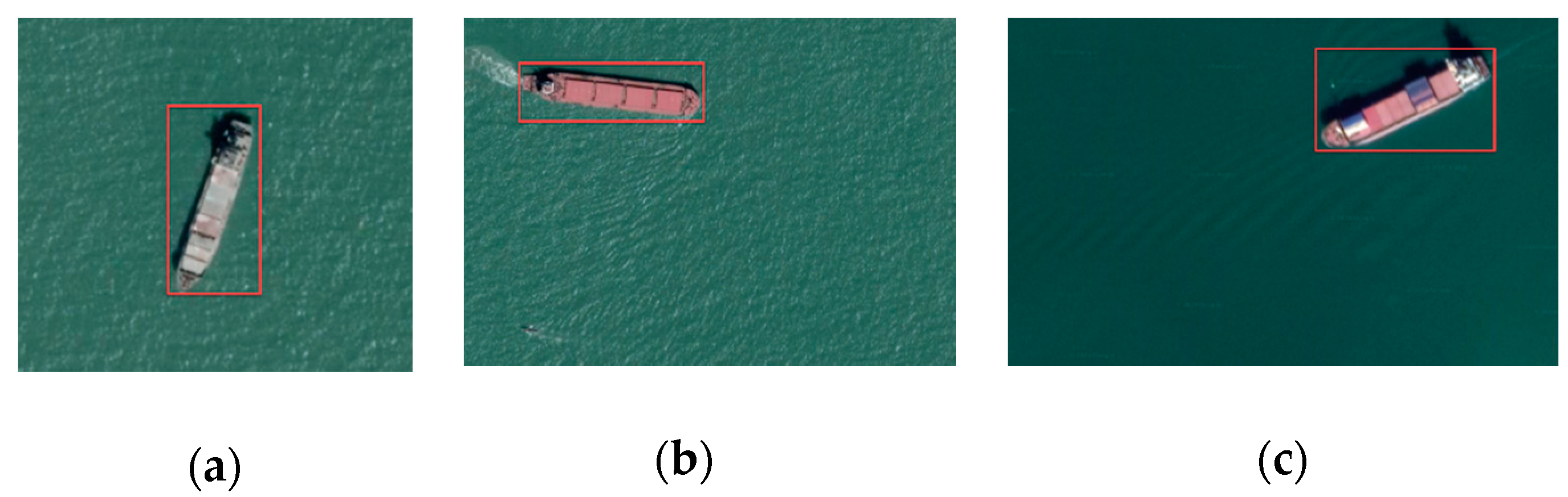
- To evaluate our proposed method’s performance on a lightweight data set that only provides limited samples, we use the HRSC2016 dataset [36]. It is a public high-resolution ship dataset that covers bounding-box labeling and three-level classes, including ship, ship category, and ship types. The HRSC2016 dataset contains images from two scenarios including ships on sea and ships close inshore. The dataset is derived from Google Earth images and associated annotations. The properties of the HRSC2016 dataset are shown in Table 1.
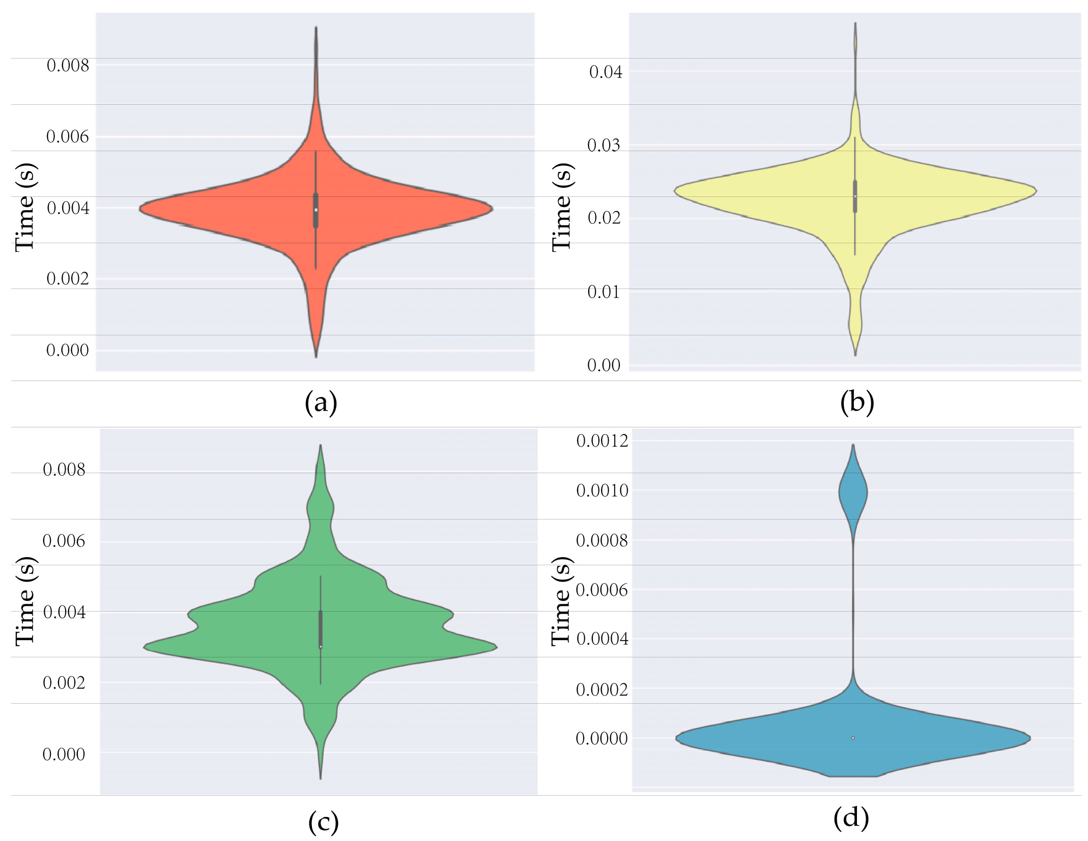
3.2. Data Analysis
4. Conclusions
Author Contributions
Funding
Conflicts of Interest
Appendix A

| Width | Height | Width | Height | Width | Height |
|---|---|---|---|---|---|
| 8 | 14 | 5 | 7 | 1 | 3 |
| 16 | 12 | 86 | 35 | 10 | 10 |
| 57 | 35 | 19 | 12 | 5 | 3 |
| 4 | 3 | 26 | 31 | 1 | 1 |
| 7 | 6 | 69 | 76 | 14 | 15 |
| 41 | 33 | 6 | 3 | 5 | 1 |
| 18 | 18 | 21 | 19 | 5 | 7 |
| 23 | 10 | 30 | 31 | 2 | 5 |
| 7 | 7 | 39 | 24 | 13 | 4 |
| 32 | 30 | 9 | 5 | 18 | 39 |
| 71 | 34 | 37 | 24 | 11 | 12 |
| 22 | 13 | 19 | 20 | 6 | 3 |
| 18 | 18 | 16 | 48 | 71 | 36 |
| 29 | 20 | 25 | 43 | 23 | 19 |
| 5 | 5 | 3 | 4 | 1 | 5 |
| 126 | 94 | 1 | 2 | 2 | 3 |
| 19 | 20 | 5 | 2 | 9 | 21 |
| 33 | 21 | 4 | 6 | 7 | 8 |
| 15 | 18 | 8 | 33 | … | … |
| Width | Height | Width | Height | Width | Height |
|---|---|---|---|---|---|
| 218 | 138 | 240 | 314 | 120 | 159 |
| 208 | 177 | 223 | 164 | 226 | 168 |
| 87 | 160 | 215 | 167 | 222 | 162 |
| 119 | 88 | 210 | 152 | 202 | 145 |
| 172 | 105 | 151 | 190 | 126 | 110 |
| 259 | 121 | 130 | 201 | 257 | 90 |
| 264 | 100 | 236 | 103 | 117 | 81 |
| 114 | 90 | 119 | 98 | 115 | 91 |
| 132 | 137 | 121 | 241 | 130 | 101 |
| 175 | 126 | 108 | 130 | 153 | 236 |
| 308 | 206 | 110 | 275 | 292 | 172 |
| 207 | 94 | 175 | 174 | 150 | 207 |
| 154 | 326 | 251 | 126 | 263 | 121 |
| 250 | 111 | 114 | 209 | 121 | 255 |
| 145 | 133 | 179 | 109 | 84 | 128 |
| 211 | 178 | 150 | 251 | 184 | 154 |
| 110 | 206 | 308 | 236 | 153 | 130 |
| 175 | 101 | 130 | 241 | … | … |
References
- Zou, Z.; Shi, Z. Ship Detection in Spaceborne Optical Image With SVD Networks. IEEE Trans. Geosci. Remote Sens. 2016, 54, 5832–5845. [Google Scholar] [CrossRef]
- Zhu, C.; Zhou, H.; Wang, R.; Guo, J. A Novel Hierarchical Method of Ship Detection from Spaceborne Optical Image Based on Shape and Texture Features. IEEE Trans. Geosci. Remote Sens. 2010, 48, 3446–3456. [Google Scholar] [CrossRef]
- Chen, H.; Gao, T.; Chen, W.; Zhang, Y.; Zhao, J. Contour Refinement and EG-GHT-Based Inshore Ship Detection in Optical Remote Sensing Image. IEEE Trans. Geosci. Remote Sens. 2019, 57, 8458–8478. [Google Scholar] [CrossRef]
- Qi, S.; Ma, J.; Lin, J.; Zhang, Y.; Tian, J. Unsupervised Ship Detection Based on Saliency and S-HOG Descriptor From Optical Satellite Images. IEEE Geosci. Remote Sens. Lett. 2015, 12, 1451–1455. [Google Scholar] [CrossRef]
- Yang, X.; Sun, H.; Fu, K.; Yang, J.; Sun, X.; Yan, M.; Guo, Z. Automatic Ship Detection in Remote Sensing Images from Google Earth of Complex Scenes Based on Multiscale Rotation Dense Feature Pyramid Networks. Remote Sens. 2018, 10, 132. [Google Scholar] [CrossRef] [Green Version]
- Li, Q.; Mou, L.; Liu, Q.; Wang, Y.; Zhu, X.X. HSF-Net: Multiscale Deep Feature Embedding for Ship Detection in Optical Remote Sensing Imagery. IEEE Trans. Geosci. Remote Sens. 2018, 56, 7147–7161. [Google Scholar] [CrossRef]
- Wang, S.; Wang, M.; Yang, S.; Jiao, L. New Hierarchical Saliency Filtering for Fast Ship Detection in High-Resolution SAR Images. IEEE Trans. Geosci. Remote Sens. 2016, 55, 351–362. [Google Scholar] [CrossRef]
- Eldhuset, K. An automatic ship and ship wake detection system for spaceborne SAR images in coastal regions. IEEE Trans. Geosci. Remote Sens. 1996, 34, 1010–1019. [Google Scholar] [CrossRef]
- Liu, C.; Gierull, C.H. A New Application for PolSAR Imagery in the Field of Moving Target Indication/Ship Detection. IEEE Trans. Geosci. Remote Sens. 2007, 45, 3426–3436. [Google Scholar] [CrossRef]
- Tello, M.; Lopez-Martinez, C.; Mallorqui, J. A Novel Algorithm for Ship Detection in SAR Imagery Based on the Wavelet Transform. IEEE Geosci. Remote Sens. Lett. 2005, 2, 201–205. [Google Scholar] [CrossRef]
- Margarit, G.; Mallorqui, J.J.; Fortuny-Guasch, J.; Lopez-Martinez, C. Exploitation of Ship Scattering in Polarimetric SAR for an Improved Classification Under High Clutter Conditions. IEEE Trans. Geosci. Remote Sens. 2009, 47, 1224–1235. [Google Scholar] [CrossRef]
- Vachon, P.; Campbell, J.; Bjerkelund, C.; Dobson, F.; Rey, M. Ship Detection by the RADARSAT SAR: Validation of Detection Model Predictions. Can. J. Remote Sens. 1997, 23, 48–59. [Google Scholar] [CrossRef]
- Morse, A.J.; Protheroe, M.A. Cover Vessel classification as part of an automated vessel traffic monitoring system using SAR data. Int. J. Remote Sens. 1997, 18, 2709–2712. [Google Scholar] [CrossRef]
- Ma, M.; Chen, J.; Liu, W.; Yang, W. Ship Classification and Detection Based on CNN Using GF-3 SAR Images. Remote Sens. 2018, 10, 2043. [Google Scholar] [CrossRef] [Green Version]
- Ai, J.; Qi, X.; Yu, W.; Deng, Y.; Liu, F.; Shi, L.; Jia, Y. A Novel Ship Wake CFAR Detection Algorithm Based on SCR Enhancement and Normalized Hough Transform. IEEE Geosci. Remote Sens. Lett. 2011, 8, 681–685. [Google Scholar] [CrossRef]
- Xu, J.; Sun, X.; Zhang, D.; Fu, K. Automatic Detection of Inshore Ships in High-Resolution Remote Sensing Images Using Robust Invariant Generalized Hough Transform. IEEE Geosci. Remote Sens. Lett. 2014, 11, 2070–2074. [Google Scholar] [CrossRef]
- Proia, N.; Page, V. Characterization of a Bayesian Ship Detection Method in Optical Satellite Images. IEEE Geosci. Remote Sens. Lett. 2010, 7, 226–230. [Google Scholar] [CrossRef]
- Ojala, T.; Pietikainen, M.; Harwood, D. Performance Evaluation of Texture Measures with Classification Based on Kullback Discrimination of Distributions. In Proceedings of the 12th International Conference on Pattern Recognition, Jerusalem, Israel, 9–13 October 1994; pp. 582–585. [Google Scholar]
- Diao, W.; Sun, X.; Zheng, X.; Dou, F.; Wang, H.; Fu, K. Efficient Saliency-Based Object Detection in Remote Sensing Images Using Deep Belief Networks. IEEE Geosci. Remote Sens. Lett. 2016, 13, 137–141. [Google Scholar] [CrossRef]
- Liu, G.; Zhang, Y.; Zheng, X.; Sun, X.; Fu, K.; Wang, H. A New Method on Inshore Ship Detection in High-Resolution Satellite Images Using Shape and Context Information. IEEE Geosci. Remote Sens. Lett. 2014, 11, 617–621. [Google Scholar] [CrossRef]
- Redmon, J.; Divvala, S.; Girshick, R.; Farhadi, A. You Only Look Once: Unified, Real-Time Object Detection. In Proceedings of the IEEE Conference on Computer Vision and Pattern Recognition (CVPR), Las Vegas, NV, USA, 27–30 June 2016; pp. 779–788. [Google Scholar]
- Redmon, J.; Farhadi, A. YOLO9000: Better, Faster, Stronger. In Proceedings of the IEEE Conference on Computer Vision and Pattern Recognition, Honolulu, HI, USA, 21–26 July 2017; pp. 7263–7271. [Google Scholar]
- Redmon, J.; Farhadi, A. Yolov3: An incremental improvement. arXiv 2018, arXiv:1804.02767. [Google Scholar]
- Bochkovskiy, A.; Wang, C.-Y.; Liao, H.-Y.M. YOLOv4: Optimal Speed and Accuracy of Object Detection. arXiv 2020, arXiv:2004.1093. [Google Scholar]
- Ren, S.; He, K.; Girshick, R.; Sun, J. Faster R-Cnn: Towards Real-Time Object Detection with Region Proposal Networks. In Proceedings of the Twenty-Ninth Conference on Neural Information Processing Systems, Montréal, QC, Canada, 7–12 December 2015; pp. 91–99. [Google Scholar]
- Cai, Z.; Fan, Q.; Feris, R.S.; Vasconcelos, N. A Unified Multi-scale Deep Convolutional Neural Network for Fast Object Detection. Comput. Vis. 2016, 9908, 354–370. [Google Scholar]
- Li, Z.; Peng, C.; Yu, G.; Zhang, X.; Deng, Y.; Sun, J. Light-Head R-Cnn: In Defense of Two-Stage Object Detector. arXiv 2017, arXiv:1711.07264. [Google Scholar]
- He, K.; Gkioxari, G.; Dollár, P.; Girshick, R. Mask R-Cnn. In Proceedings of the IEEE International Conference on Computer Vision, Venice, Italy, 22–29 October 2017; pp. 2961–2969. [Google Scholar]
- He, K.; Zhang, X.; Ren, S.; Sun, J. Spatial pyramid pooling in deep convolutional networks for visual recognition. IEEE Trans. Pattern Anal. Mach. Intell. 2015, 37, 1904–1916. [Google Scholar]
- Girshick, R. Fast R-CNN. In Proceedings of the 2015 IEEE International Conference on Computer Vision (ICCV), Santiago, Chile, 7–13 December 2015; pp. 1440–1448. [Google Scholar]
- Girshick, R.; Donahue, J.; Darrell, T.; Malik, J. Rich Feature Hierarchies for Accurate Object Detection and Semantic Segmentation. In Proceedings of the 2014 IEEE Conference on Computer Vision and Pattern Recognition, Columbus, OH, USA, 23–28 June 2014; pp. 580–587. [Google Scholar]
- Liu, Z.; Hu, J.; Weng, L.; Yang, Y. Rotated region based CNN for ship detection. In Proceedings of the 2017 IEEE International Conference on Image Processing (ICIP), Beijing, China, 17–20 September 2017; pp. 900–904. [Google Scholar]
- Li, L.; Zhou, Z.; Wang, B.; Miao, L.; Zong, H. A Novel CNN-Based Method for Accurate Ship Detection in HR Optical Remote Sensing Images via Rotated Bounding Box. IEEE Trans. Geosci. Remote Sens. 2020, 1–14. [Google Scholar] [CrossRef]
- Cucchiara, R.; Crana, C.; Piccardi, M.; Prati, A.; Sirotti, S. Improving shadow suppression in moving object detection with HSV color information. IEEE Intell. Transp. Syst. 2002, 334–339. [Google Scholar] [CrossRef]
- Shaik, K.B.; Ganesan, P.; Kalist, V.; Sathish, B.; Jenitha, J.M.M. Comparative Study of Skin Color Detection and Segmentation in HSV and YCbCr Color Space. Procedia Comput. Sci. 2015, 57, 41–48. [Google Scholar] [CrossRef] [Green Version]
- Liu, Z.; Yuan, L.; Weng, L.; Yang, Y. A High Resolution Optical Satellite Image Dataset for Ship Recognition and Some New Baselines. In Proceedings of the 6th International Conference on Pattern Recognition Applications and Methods, Porto, Portugal, 24–26 February 2017. [Google Scholar]


| Properties | Value |
|---|---|
| Image resolution | 0.4 m–2 m |
| Image size | 300 × 300 − 1500 × 900 |
| Total image | 1061 (with annotations) 610 (without annotations) |
Publisher’s Note: MDPI stays neutral with regard to jurisdictional claims in published maps and institutional affiliations. |
© 2020 by the authors. Licensee MDPI, Basel, Switzerland. This article is an open access article distributed under the terms and conditions of the Creative Commons Attribution (CC BY) license (http://creativecommons.org/licenses/by/4.0/).
Share and Cite
Tang, G.; Liu, S.; Fujino, I.; Claramunt, C.; Wang, Y.; Men, S. H-YOLO: A Single-Shot Ship Detection Approach Based on Region of Interest Preselected Network. Remote Sens. 2020, 12, 4192. https://0-doi-org.brum.beds.ac.uk/10.3390/rs12244192
Tang G, Liu S, Fujino I, Claramunt C, Wang Y, Men S. H-YOLO: A Single-Shot Ship Detection Approach Based on Region of Interest Preselected Network. Remote Sensing. 2020; 12(24):4192. https://0-doi-org.brum.beds.ac.uk/10.3390/rs12244192
Chicago/Turabian StyleTang, Gang, Shibo Liu, Iwao Fujino, Christophe Claramunt, Yide Wang, and Shaoyang Men. 2020. "H-YOLO: A Single-Shot Ship Detection Approach Based on Region of Interest Preselected Network" Remote Sensing 12, no. 24: 4192. https://0-doi-org.brum.beds.ac.uk/10.3390/rs12244192