Article

Tree Cover Estimation in Global Drylands from Space Using Deep Learning

by
Emilio Guirado
1,2,3,*,
Domingo Alcaraz-Segura
3,4,5,
Javier Cabello
3,6,
Sergio Puertas-Ruíz
4,
Francisco Herrera
1 and
Siham Tabik
1
1
Andalusian Research Institute in Data Science and Computational Intelligence, University of Granada, 18071 Granada, Spain
2
Multidisciplinary Institute for Environment Studies “Ramón Margalef”, University of Alicante, San Vicente del Raspeig, 03690 Alicante, Spain
3
Andalusian Center for Assessment and Monitoring of Global Change (CAESCG), University of Almería, 04120 Almería, Spain
4
Department of Botany, Faculty of Science, University of Granada, 18071 Granada, Spain
5
Iecolab. Inter-University Institute for Earth System Research, University of Granada, 18006 Granada, Spain
6
Department of Biology and Geology, University of Almería, 04120 Almería, Spain
*
Author to whom correspondence should be addressed.
Submission received: 4 December 2019 / Revised: 31 December 2019 / Accepted: 15 January 2020 / Published: 21 January 2020

Abstract

:
Accurate tree cover mapping is of paramount importance in many fields, from biodiversity conservation to carbon stock estimation, ecohydrology, erosion control, or Earth system modelling. Despite this importance, there is still uncertainty about global forest cover, particularly in drylands. Recently, the Food and Agriculture Organization of the United Nations (FAO) conducted a costly global assessment of dryland forest cover through the visual interpretation of orthoimages using the Collect Earth software, involving hundreds of operators from around the world. Our study proposes a new automatic method for estimating tree cover using artificial intelligence and free orthoimages. Our results show that our tree cover classification model, based on convolutional neural networks (CNN), is 23% more accurate than the manual visual interpretation used by FAO, reaching up to 79% overall accuracy. The smallest differences between the two methods occurred in the driest regions, but disagreement increased with the percentage of tree cover. The application of CNNs could be used to improve and reduce the cost of tree cover maps from the local to the global scale, with broad implications for research and management.

Graphical Abstract

1. Introduction

Making accurate estimates of tree cover with affordable methods and available data across vast regions is critical in many fields, such as carbon stocks and biomass estimation [1,2,3,4,5], biodiversity assessment [6,7], ecohydrological modelling [8], Earth system modelling [9,10,11], forestry [12], and ecological succession [13,14]. The role of tree cover in stabilizing the carbon cycle in drylands is particularly relevant, give their capacity to buffer the seasonal and interannual variability in precipitation [15]. Reducing uncertainties about the extent, distribution, and tree cover of forests in dryland biomes [16,17] is particularly necessary given the huge contribution of drylands to the interannual variability of the global carbon cycle [18]. To address these uncertainties, the FAO (Food and Agriculture Organization of the United Nations) recently conducted the Global Drylands Assessment (GDA), a costly study that assessed the forest cover of dryland forests around the world [19].
FAO’s GDA expanded the extent of tree cover in dryland biomes by 9% [19] compared to previous studies. Such differences in tree cover were particularly important for regions with a high proportion of open forest (10–40% tree cover), but also for those areas with closed forest cover (≥40% tree cover) [20]. Discrepancies in tree cover estimation can be explained by the different methodologies used for estimating tree cover, which include images with different spatial resolutions (mainly very high resolution versus mainly Landsat [21] or MODIS [22,23] images), and the use of different image processing methods (automatic algorithms versus manual photointerpretation, [16,19,20,21,22,23,24]). FAO’s GDA used the augmented visual interpretation method (implemented in the Collect Earth software) on very high resolution images (VHR) from Google EarthTM. However, FAO’s GDA was controversial and several studies raised many sources of uncertainty [25,26,27,28,29], mainly related to soil background effects and to the biases and subjectivities introduced by hundreds of operators worldwide. In any case, FAO’s GDA required a vast effort, which limits the use of this methodology for monitoring. Hence, there still exists a need to develop more cost-effective, faster, less subjective and more precise methods to reduce uncertainty in estimating tree cover in global drylands [30,31,32].
Recent studies have demonstrated the potential of convolutional neural networks (CNNs) in remote sensing (e.g., [33]) for land cover mapping using aerial and satellite imagery (e.g., scattered shrub detection [30], crop type classification, land use and land cover mapping, and change detection [34,35,36,37,38]). CNNs, a type of deep-learning method within artificial intelligence, are the dominant and most accurate methods in recognition and detection in images [39]. Since 2014, the quality of CNN architectures has considerably improved thanks to deeper and broader networks [40]. CNNs such as GoogLeNet Inception can achieve accuracies of over 90%, when trained on high quality datasets, operate under strict memory and computational processing capacity constraints, and are increasingly used in remote sensing [41]. For example, Inception v.3 [42], the model that won the ILSVRC 2016 (ImageNet Large Scale Visual Recognition Competition), is now one of the most widely used CNNs.
Image classification based on deep learning has been proved to improve the speed and accuracy reached by manual labelling [43,44,45]. CNNs have been used to classify different land uses with well-defined classes in satellite images [46]. However, in continuous classifications, such as the estimation of the percentage of tree cover, artificial intelligence based on deep learning has been used in few studies (e.g., biomass estimation [47]). Our study proposes the use of CNNs to develop an automatic method for quantifying forest cover in drylands using very high resolution satellite and aerial images (such as the RGB images of the Earth surface provided by Google EarthTM software, https://google.com/earth). Then, we compared the performance of our CNN-based method with the approach of the FAO’s Global Dryland Assessment, which is based on manual visual interpretation using Collect Earth by human technicians [19]. Our main hypothesis is that the estimation of tree cover using a CNN-based model would be more accurate and less biased than FAO’s assessment using manual visual interpretation. To do this, we first compared the effect of different strategies to design the training datasets on the ability of the CNN in differentiating three tree cover classes (open, close, and dense forest; see Figure 1 and Figure S2): i.e., (1) by including a non-forest auxiliary class with many more samples than the targeted tree cover classes, (2) by considering samples along continuous tree cover levels within each class versus samples taken only at a discrete tree cover level within each class, and (3) by increasing the size of the training dataset. Second, we used the best trained CNN model to quantify tree cover on a representative sample of plots in the FAO’s GDA. Finally, the accuracy of tree cover quantification was compared between the CNN-based method and the FAO’s GDA [19].
The main contributions of this paper can be summarized as follows:
  • Finding a dataset design and learning strategy that makes the CNN model correctly learn and predict tree cover in orthoimages. In particular, we showed how (1) adding to the training dataset an auxiliary “non-forest” class with many more samples than the targeted classes negatively affected performance; (2) selecting training samples along the continuous range of tree cover percentages within each class achieved greater performance than selecting samples at a discrete percentage; and (3) increasing the number of samples in the targeted tree-cover classes of the training dataset did not significantly affect performance.
  • Demonstrating as a proof of concept that CNN models can estimate tree cover in orthoimages with better accuracy than FAO’s GDA based on manual land cover classification in Collect Earth.

2. Materials and Methods
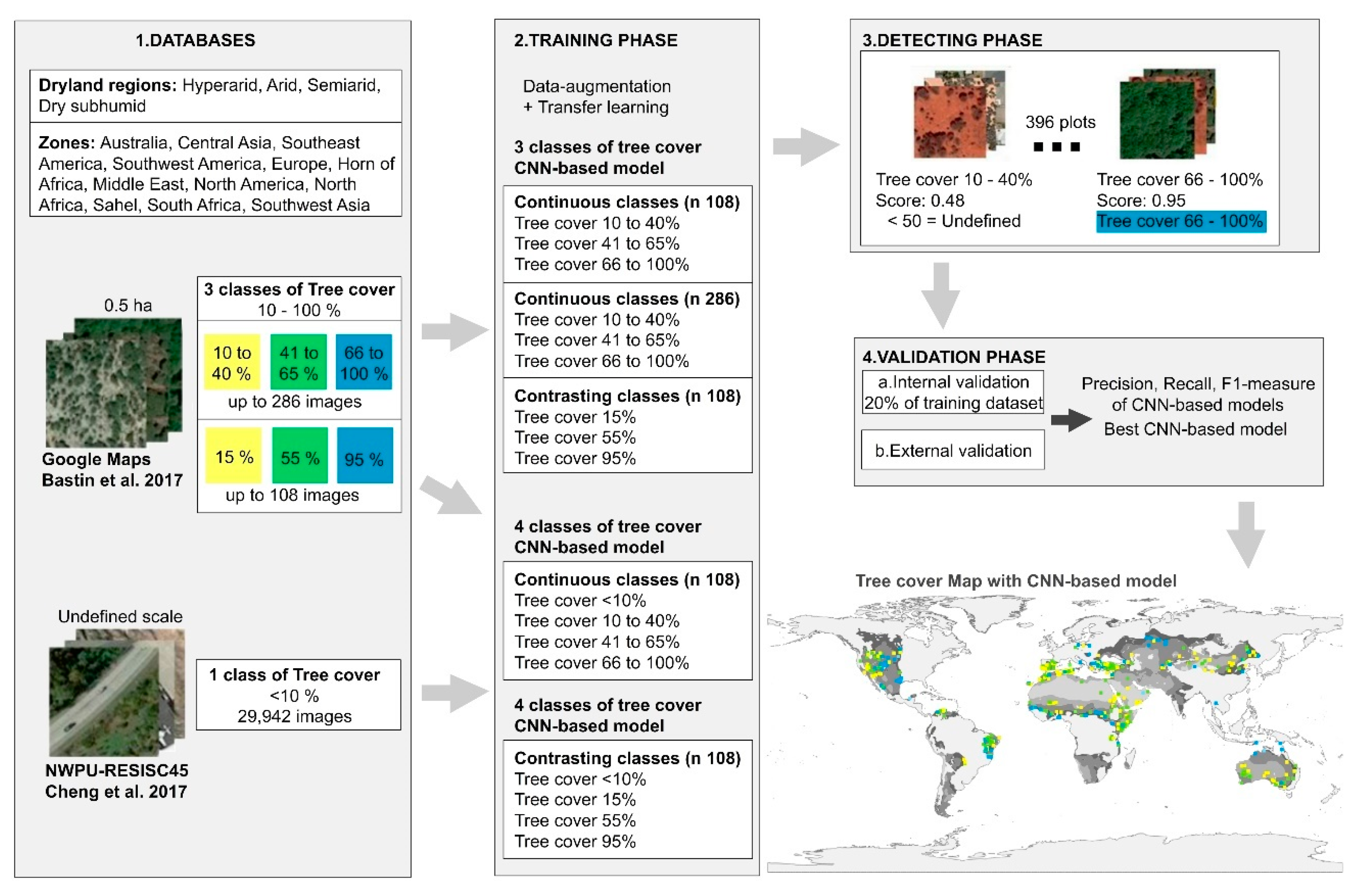
The problem of estimating tree cover in global drylands with deep learning by means of an image classification model was addressed as a proof-of-concept of how convolutional neural networks can provide more accurate estimates of tree cover than visual photointerpretation made by humans. To build the CNN-based model of tree cover, we used the Inception v.3 [42,43] image recognition model, one of the most widely used CNNs (see Supplementary Material, Figure S1), with TensorFlow (Section 2.3, Section 2.4, and Section 2.5). CNN-based models learn directly from image data, eliminating the manual determination of spectral and spatial characteristics that define the classes of objects or units to be identified in the image (e.g., tree cover classes). To compare CNN’s performance to FAO’s GDA photointerpretation through Collect Earth [19], we assessed a representative sample of plots from FAO’s GDA, stratified across 12 geographical areas, four levels of aridity, and four levels of tree cover (Table S1), as in [19]. The 12 dryland regions were: Australia, Central Asia, Southeastern America, Southwestern America, Europe, Horn of Africa, Middle East, North America, North Africa, Sahel, South Africa, and Southwest Asia. The four aridity levels were based on the aridity index (AI: ratio between total annual precipitation and potential evapotranspiration): hyperarid (AI < 0.05), arid (0.05 ≤ AI < 0.2), semiarid (0.2 ≤ AI < 0.5) and dry subhumid (0.5 ≤ AI < 0.65)., The four tree cover classes were: Non-Forest (<10%), Open Forest (10–40%), Closed Forest (41–65%), and Dense Forest (66–100%).

2.1. Workflow

To build the CNN-based method for tree cover estimation, we followed four phases (Figure 1):
(1)
Database construction phase: five training datasets were built with examples of images with different levels of tree cover, continuous and discrete approximations, and inclusion of auxiliary class “Non-Forest” (see Section 2.2 and Supplementary Material, Archive S2).
(2)
Training phase: training five CNN models based on Inception v.3 using two optimization techniques, transfer learning, and data augmentation (see Section 2.3).
(3)
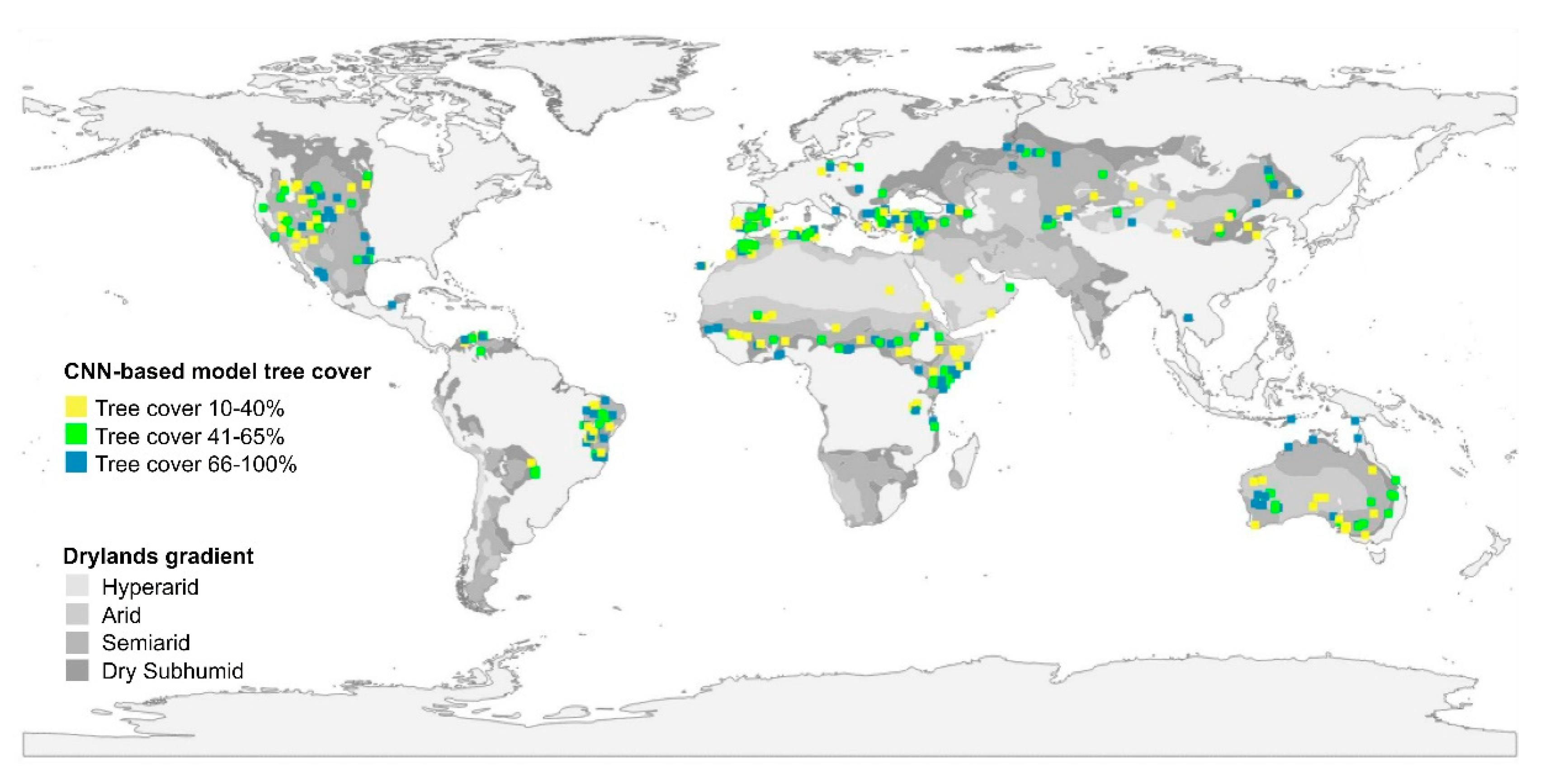
Classification phase: classification of new 396 images with different tree cover in global drylands (see Supplementary Material, Table S1 and Archive S3) with the built CNN-based model (see Section 2.4).
(4)
Validation phase: assessment of performance on the new images (see Section 2.5).

2.2. Datasets Design

Before building the training datasets for the CNN-based models, we compiled a global database of very high resolution satellite and aerial RGB images from two sources:
  • First, we downloaded 71,135 images from Google Maps corresponding to the FAO’s GDA 0.5 ha forest and non-forest plots that were available at zoom 19 (eye altitude ~150 m and pixel ~0.5 m). Download occurred between 1 and 13 December 2017 (see Supplementary Material, Archive S1). In FAO’s GDA, each plot is georeferenced and tagged as forest or non-forest, with a tree cover percentage, and with a climate and region of the world [19].
  • Second, to increase the number of images in the “Non-Forest” class, we used the Northwestern Polytechnical University NWPU-RESISC45 dataset [48], a set of publicly available reference orthoimages for the classification of remotely sensed images, developed by NWPU. This dataset contains 31,500 images with 45 different scene classes (i.e., land use, land cover, objects, and infrastructure) with 700 images within each class. To build our global dataset, we removed all images corresponding to the “chaparral” and “forest” classes and grouped the remaining classes. We then reviewed all these images and filtered noisy ones. We obtained a total of 29,942 images that met FAO’s criteria for Non-Forest (e.g., roads, rivers, beaches, urban areas, etc.).
Once the global database was compiled, we created five different training datasets to compare the effect of five different learning strategies on the performance of the CNN-based model (Table 1). The selection of forest images from our database was stratified across the different combinations of regions, aridity levels, and tree cover levels used by FAO [19] (Supplementary Material, Table S1). The five created datasets contained three tree cover classes: Open Forest, Closed Forest, and Dense Forest (Figure S2). In the continuous strategy, we built each tree cover class by selecting training samples along the continuous range of tree cover percentages. While in the discrete strategy, we built each tree cover class by selecting samples only at a discrete percentage of tree cover (the 15%, 55%, and 95% levels were used to maximize the distance and contrast between classes, i.e., 40% difference in tree cover percentage among them). We also included a “Non-Forest” class in two of the datasets (see Section 2.4 for a description of the images contained in each dataset).

2.3. Training Phase: CNN-Based Model Parameters

To build a CNN-based model able to accurately estimate tree cover in a given input image, we evaluated different training strategies. In particular, we considered continuous and discrete learning. In the continuous learning, the model is trained to estimate an interval of tree cover, e.g., Open Forest with tree cover from 10% to 40%. In discrete learning, the model is trained to estimate the exact tree cover, e.g., Open Forest with 15% tree cover. We also evaluated considering a “Non-Forest” class in the training. In total, we designed five datasets (see Table 1).
For this, we obtained five models by training Inception v.3 on the five created datasets. Several studies have shown that increasing the size of the dataset using data augmentation improves the performance of the CNN-based models [49,50]. These techniques have been proposed to reduce the requirement of a large dataset for model training [43,44,45]. We configured the model parameters by training the last two fully connected network layers in our dataset using a learning rate of 0.001 and a decay factor of 16 every 30 epochs. As an optimization algorithm, we used RMSProp with a momentum of 0.9 and epsilon of 0.1.
In the training phase, data-augmentation technique was used to artificially increase the number of samples [50]. Data augmentation apply specific transformations to the original samples, but preserving their labels to obtain samples slightly different from the original ones [50]. In particular, a 50% increase in brightness, half-random rotation, random rotation with a factor randomly selected between 0º and 359º, random cropping, and random scale of image size were used. In addition, we used transfer learning to reuse the knowledge acquired by the CNN model in a first problem to apply it to another related problem. Transfer learning is analogous to the development of knowledge in humans, which never starts from scratch, as it is always done from previous knowledge. We used the pretrained weights on ImageNet database to initialize the Inception v.3 model. ImageNet has 1.28 million images for 1000 different classes of objects [51].

2.4. Optimizing a CNN-Based Model to Detect Tree Cover Classes

In the classification phase, the CNN-based model provided for each image the probability (0–100%) of belonging to each class. The prediction of CNN-based model for each image had to be 50% or higher probability to be used in further analysis. Otherwise, we considered the prediction to be uncertain and was not taken into account.
To determine which of the five CNN-based models was the best estimated tree cover, each of them had a dataset built differently (see below in this section). To assess whether the “continuous tree cover” versus “discrete tree cover” categories increased the model’s performance during the training phase, we tested two different strategies for constructing tree cover categories. In the first case, we defined continuous categories considering the following three tree cover intervals: 10–40% for Open Forest, 41–65% for Closed Forest, and 66–100% for Dense Forest classes [52]. In the case of the discrete categories, we selected three tree cover classes with maximum separation of tree cover with 40% constructed as images of Open Forest with 15% tree cover, Closed Forest with 55%, and Dense Forest with 95%. Therefore, there were five possible combinations (five different) regarding the type of CNN-based model training datasets (Table 1). In addition, we evaluated whether a Non-Forest class with tens of thousands of training images facilitates the classification of tree cover in drylands. Finally, success rates were compared between the CNN-based model trained without a Non-Forest class and with a Non-Forest class that contained 29,942 non-forest images from the NWPU-RESISC45 dataset [48].

2.5. Validation of the CNN-Based Model

To validate the CNN-based models, we built a final dataset of the 396 images from 71,135 Google Maps VHR images of FAO’s GDA plots. We selected the images with samples stratified across different combinations of regions, aridity levels, and tree cover, according to FAO [19]. Thus, to get answers to these combinations in the 71,135 images downloaded with zoom 19 from Google Maps, we tried to choose a minimum of three images and a maximum of seven. However, this was not always possible, resulting in a dataset with a total of 396 images (Table S1 and Archive S3). Two evaluators (authors) established Forest or Non-Forest tags and tree cover for each image in the external dataset. The evaluators were trained to perform the visual interpretation of the tree cover level of the images. Therefore, the labels assigned by them were used in the external validation as a reference for a correct classification. Hence, two validation procedures were performed: internal and external. First, the internal validation used the performance obtained by classifying 20% of the images from the training dataset (while 80% was used in the training phase). Second, external validation was carried out independently of the training dataset.
To evaluate the performance of both CNN-based models, we used these metrics [30]: precision (Equation (1)), recall (Equation (2)), and F1-measure (Equation (3)):
Precision   =   T r u e   p o s i t i v e s T r u e   p o s i t i v e s + F a l s e   p o s i t i v e s   ,
Recall   =   T r u e   p o s i t i v e s T r u e   p o s i t i v e s + F a l s e   n e g a t i v e s   ,
F 1 - measure   =   2   ×   P r e c i s i o n   ×   R e c a l l P r e c i s i o n + R e c a l l   ,
where false positives represent the images that were classified by the models but actually corresponded to another class, true positives represent the images that were correctly classified by the model, and false negatives represent the images not detected by the model. In simple terms, the high positive predictive value means that the model returned substantially better tree cover classes, while the high sensitivity means that the model returned most of the actual tree cover. The F1-measure provides a balance between sensitivity and precision. We used five-fold cross-validation strategy to evaluate our approach and the baseline on the test dataset.

3. Results

3.1. Effect of CNN Training Strategies on Performance to Estimating Tree Cover in Drylands

The lowest F1-measure for tree cover classification was observed in the two models trained with the datasets that included the Non-Forest class. Regarding the models trained on datasets of the same size that did not include a Non-Forest class (rows 2 and 3 in Figure 2), the CNN-based model with continuous categories obtained a higher F1-measure than the CNN-based model trained with discrete categories. The improvement in F1-measure thanks to the use of continuous categories in the training dataset was large (up to 6%) in Dense forest, null (0%) in Closed forest, and small (2%) in Open forest (Figure 2).
The increase in the size of the training dataset improved model performance. The most accurate CNN-based model was obtained without the Non-Forest auxiliary class, using continuous tree cover classes, and a larger number of training samples (see Table 1). This model reached the highest F1-measure for Open Forest and Dense Forest, 71% and 79%, respectively. The CNN-based model with the largest number of samples showed an increase in the F1-measure compared to the CNN-based model with a smaller number of samples, up to 1% for Open Forest, and Dense Forest (Figure 2).
In summary, the FAO’s GDA manual photointerpretation method using Collect Earth [19] always showed lower accuracy than the CNN-based model for the selected dataset in all tree cover classes. For Open, Close, and Dense Forest classes according to the best CNN-based model, the respective F1-measures were higher (71%, 53%, and 79%) than FAO’s assessment (54%, 30%, and 52%) (Figure 3 and Table S2).

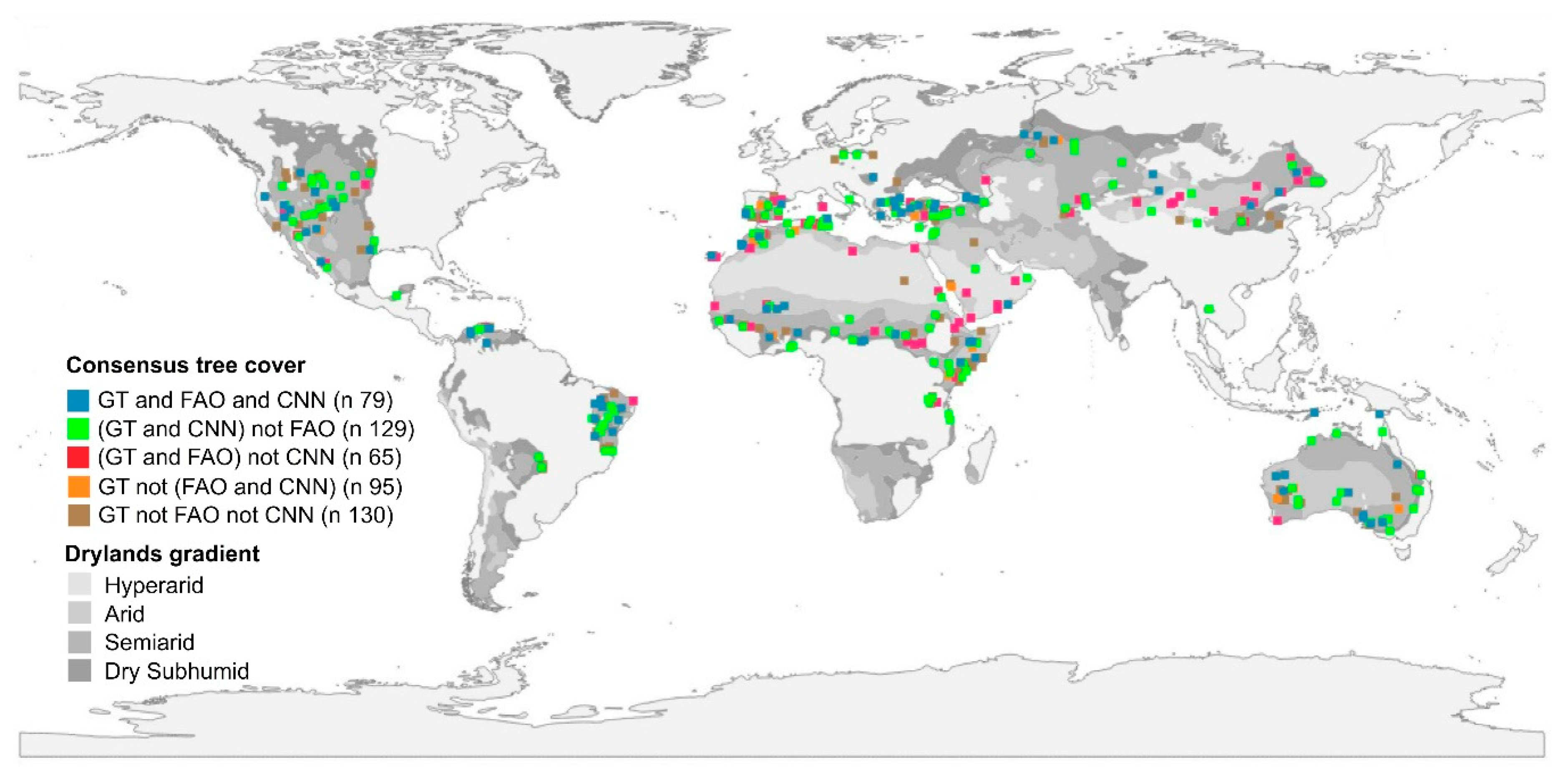
3.2. Differences between the Best CNN-Based Model and FAO’s Global Dryland Assessment

Full consensus of correctly estimated tree cover classes between the best CNN-based model and FAO’s GDA assessment only occurred in 79 plots (Figure 4), 22% of the total dataset (Table 2). The number of correctly estimated tree cover classes just by CNN-based models was higher (129) than the number correctly estimated just by FAO’s GDA (65).
Regarding aridity gradient, the disagreements between FAO’s GDA assessment and the best CNN-based model were 4.7%, 15.3%, 24.5%, and 27.6% of F1-measure in hyperarid, arid, semiarid, and dry subhumid, respectively (Table 2).

4. Discussion

4.1. CNNs to Estimate Tree Cover in Drylands

Our results showed that the automatic classification of tree cover in satellite VHR RGB images in drylands with CNNs was more effective than the manual photointerpretation method of Collect Earth used by FAO’s GDA, which employed hundreds of operators. The greater performance of CNNs compared to human visual interpretation has also been reported in other studies (e.g., [43,44,45]). Our results call for further improvements in our CNN method by using more images in the training dataset and increasing their quality (e.g., spatial resolution) and representativeness in all global environmental gradients.
Many studies show how deep-learning classification is a powerful tool for land cover and crop types using remote sensing data [53,54], detection of individual trees in RGB images [55], identification of tree species related to forest disturbance with very high resolution multispectral images [56], and detection of firs damaged by bark beetle in unmanned aerial vehicle (UAV) images [57]. However, the studies to detect the percentage of land use surface, is addressed by segmentation methods such as Mask-RCNN [58] with high computational cost [59]. In this study, tree cover estimation is approached from a simple classification method [42] with better results than manual methods [19]. In addition, we observed that increasing the training data set improves the accuracy of the classification (e.g., [60,61]); however, our results showed that increasing the training data on the tree cover estimation problem, increasing training data by 165%, only improved the F1-measure to 1% in two of the three classes studied (Tree cover 10–40% and Tree cover 66–100%).
Intermediate tree cover (Closed Forest class) was worse estimated both by the Collect Earth manual approach and CNN-based methods compared with low tree cover (Open Forest) and high tree cover (Dense Forest). This is due to their intermediate position between the Open Forest and Dense Forest classes, with similarity for both classes. In fact, many studies only use two forest density categories, such as open and dense forest (e.g., [62,63,64]), even for assessing transitional forests [65] or even just one closed forest class [66]. This similarity of our Close Forest class to the surrounding Open and Dense forest classes could confuse the identifiable patterns of Closed Forest with the other two classes by the CNN-based models. In addition, the comparison between the FAO’s GDA method and the best CNN-based model could have involuntary classification errors, due to human failures in the photointerpretation of the plots or to an update of the images in Google Maps (between FAO’s assessment and ours) that would show changes in tree cover. Since the accuracy (F1-measure) of FAO’s GDA tree cover estimation is relatively low [26,27,28], we should not expect high consensus with any method that has high accuracy. If a high consensus exists, it would imply that the new method is as inaccurate as FAO’s GDA [19].
The CNN-based model was more effective when the training dataset did not include a Non-Forest class, which can be understood as a decrease in background noise [67]. So, the learning was more oriented towards the proposed goal: the quantification of the tree cover of forest (e.g., [68,69]). The CNN-based models trained with continuous categories showed a high F1-measure probably because they were trained with more diverse and varied examples to characterize each class of tree cover, except the Closed Forest class, as previously discussed. The CNN-based models trained with discrete categories presented low F1-measure probably due to the variability between the training samples was lower than using continuous categories.

4.2. Limitations and Challenges in Tree Cover Mapping

The main limitation found in this work was of a technical nature. Despite the current increase in the number of very high resolution satellite sensors (e.g., [70,71,72]), there are still many parts of the Earth’s surface that are not yet covered by VHR images (e.g., remote areas). For example, there is low availability of VHR images in Africa while high availability in Australia [73]. This means that we could not design a larger training dataset for each class (even if we used data augmentation and transfer learning) in CNN-based models [74]. Other technical difficulties for the application of CNNs on satellite images to estimate tree cover at the global scale are the vast amount of data to handle [75], and the need for graphics processing unit (GPU) servers to efficiently train the CNN models [76].
Traditionally, forest cover is often estimated by surrogates of vegetation structure (e.g., leaf area index, phytolith index [77]). Many studies have assessed tree cover from local to global scales through the use of normalized difference vegetation index (NDVI) images from the MODIS (moderate resolution image spectroradiometer) and Landsat satellite sensors, in both cases with high accuracies [15,18,20,22]..
In addition, as a complement to these methods, CNN-based methods could provide new information for a more accurate estimate of tree cover and, subsequently of net carbon gains [78], biodiversity [79], or forest health [80]. A global application of our CNN-based model on VHR satellite images to estimate tree cover in drylands could greatly complement traditional tree cover mapping methods [16,20,22]. Increased tree-cover estimation accuracies would also help to characterize forest areas affected by environmental and anthropogenic changes (e.g., [81,82]), or to set priorities for protecting biodiversity from global change [83,84,85]. The use of CNNs is useful due to their automatic character; once built and trained, it can be used as a classifier of new images without another training phase. In addition, CNNs have the favorable characteristic of being able to learn and reuse learning from one image to another [49], this characteristic makes them versatile at a planetary scale. For example, the application of CNN-based model of tree cover detectors on VHR satellite images could be used to through a global community involved as part of the Group on Earth Observations–Biodiversity Observation Network (GEOBON) initiative on essential biodiversity variables from satellite remote sensing [86].

5. Conclusions

Dry forests have global importance. However, there is still high uncertainty about their extent and tree cover. Our research shows how the development and implementation of a new free and automatic tools using CNN-based models on very high resolution and free aerial and satellite RGB imagery could be used to quantify the tree cover of forests in global drylands. Compared to Collect Earth manual method used in the FAO’s Global Drylands Assessment, the CNN-based model has demonstrated greater accuracy (by 23% better) and speed. We encourage further development and application of this technology in future works at local, regional, continental, or global scales to increase the accuracy of forest tree cover estimation in drylands, from researchers to organizations (e.g., FAO). More accurate tree cover mapping based on CNN models would positively impact many fields, from biodiversity conservation to carbon stock estimation, ecohydrology, erosion control, or Earth system modelling.

Supplementary Materials

The following are available online at https://0-www-mdpi-com.brum.beds.ac.uk/2072-4292/12/3/343/s1, Figure S1: Number of results in the Google scholar academic search engine. Date of queries, 28 December 2019. [keyword + deep learning]. Keywords: AlexNet, DenseNet, GoogLeNet, Inception, MobileNet, Resnet, Resnext, VGG, Xception. Figure S2: Illustration of the difference between the sampling design strategies, (A) Continuous and (B) Discrete, including examples of images (0.5 ha) from each class (Three Tree-Cover levels plus the Non-Forest class) of the training dataset. Image data: Google, Maxar, and NWPU-RESISC45 dataset. Archive S1: Metadata of FAO’s GDA photointerpreted very high resolution plots (71,135) with zoom 19 in Google Maps. The CVS file contains Id, UpperLeft and Downright coordinates, Zoom, Region, Aridity level, Class (Forest/Non-forest), and Tree cover. Archive S2: Metadata of training dataset of continuous larger sample CNN-based model with very high resolution plots (286) and zoom 19 in Google Maps. The CVS file contains Id, UpperLeft and Downright coordinates, Zoom, Region, Aridity level, Class (Forest/Non-Forest), and Tree cover. Archive S3: Metadata of the results of CNN-based models in 396 plots. The CVS file contains Id, UpperLeft and Downright coordinates, Region, Aridity level, Class (Forest/Non-Forest), and Tree cover. Consensus results. Precision, Recall, and F1-measure. Table S1: Representativeness of the database for external validation of the CNN-method that classifies orthoimages into tree cover classes. A total of 396 images were sampled globally stratified across the different combinations of regions, aridity levels, tree cover levels and forest and non-forest classes according to Bastin et al. (2017). Some combinations did not exist or did not have images with good quality. NF (Non-Forest), F(Forest), TC (Tree cover). Table S2: Precision, Recall and F1-measure of CNN-based models. True positives (TP), false positives (FP), and false negatives (FN). F1-measure provides a balance between precision and sensitivity.

Author Contributions

E.G., S.T., S.P.-R., and D.A.-S. designed the experiments, collected the data, and analyzed the results; E.G. and S.T. implemented the code and ran the models; E.G., S.P.-R., and D.A.-S. wrote the first draft; F.H., J.C., S.T., E.G., and D.A.-S. revised the final manuscript. All authors have read and agreed to the published version of the manuscript.

Funding

S.T., E.G., D.A.-S., and F.H. were supported by the project DeepSCOP-Ayudas Fundación BBVA a Equipos de Investigación Científica en Big Data 2018. E.G. is supported by the European Research Council grant agreement 647038 (BIODESERT). S.T. is supported by the Ramón y Cajal Program of the Spanish Government (RYC-2015-18136). S.T., E.G., and F.H. were supported by the Spanish Ministry of Science under the project TIN2017-89517-P. D.A.-S., E.G., and J.C. received support from project ECOPOTENTIAL, funded by European Union Horizon 2020 Research and Innovation Program, under grant agreement No. 641762, and from European LIFE Project ADAPTAMED LIFE14 CCA/ES/000612. D.A-S, S.T. and E.G. received support from Programa Operativo FEDER-Andalucía 2014-2020 under project DETECTOR A-RNM-256-UGR18. D.A-S. received support from NASA’s Work Program on Group on Earth Observations—Biodiversity Observation Network (GEOBON) under grant 80NSSC18K0446.

Acknowledgments

We are grateful to Javier Montes for providing help with the Python scripts to access Google Maps’ API.

Conflicts of Interest

The authors declare no conflict of interest.

References

  1. Popescu, S.C.; Wynne, R.H.; Nelson, R.F. Measuring individual tree crown diameter with lidar and assessing its influence on estimating forest volume and biomass. Can. Aeronaut. Space J. 2003, 29, 564–577. [Google Scholar] [CrossRef]
  2. Karlson, M.; Ostwald, M.; Reese, H.; Sanou, J.; Tankoano, B.; Mattsson, E. Mapping tree canopy cover and aboveground biomass in Sudano-Sahelian woodlands using Landsat 8 and random forest. Remote Sens. 2015, 7, 10017–10041. [Google Scholar] [CrossRef] [Green Version]
  3. Hall, J.M.; Van Holt, T.; Daniels, A.E.; Balthazar, V.; Lambin, E.F. Trade-offs between tree cover, carbon storage and floristic biodiversity in reforesting landscapes. Landsc. Ecol. 2012, 27, 1135–1147. [Google Scholar] [CrossRef]
  4. Achard, F.; Beuchle, R.; Mayaux, P.; Stibig, H.J.; Bodart, C.; Brink, A.; Lupi, A.; Carboni, S.; Desclée, B.; Donnay, F.; et al. Determination of tropical deforestation rates and related carbon losses from 1990 to 2010. Glob. Chang. Biol. 2014, 20, 2540–2554. [Google Scholar] [CrossRef] [PubMed]
  5. Huang, C.Y.; Asner, G.P.; Martin, R.E.; Barger, N.N.; Neff, J.C. Multiscale analysis of tree cover and aboveground carbon stocks in pinyon–juniper woodlands. Ecol. Appl. 2009, 19, 668–681. [Google Scholar] [CrossRef] [PubMed] [Green Version]
  6. Prevedello, J.A.; Almeida-Gomes, M.; Lindenmayer, D.B. The importance of scattered trees for biodiversity conservation: A global meta-analysis. J. Appl. Ecol. 2018, 55, 205–214. [Google Scholar] [CrossRef]
  7. Sexton, J.O.; Noojipady, P.; Song, X.P.; Feng, M.; Song, D.X.; Kim, D.H.; Anand, A.; Huang, C.; Channan, S.; Pimm, S.L.; et al. Conservation policy and the measurement of forests. Nat. Clim. Chang. 2016, 6, 192. [Google Scholar] [CrossRef]
  8. Joffre, R.; Rambal, S. How tree cover influences the water balance of Mediterranean rangelands. Ecology 1993, 74, 570–582. [Google Scholar] [CrossRef]
  9. Xu, X.; Medvigy, D.; Trugman, A.T.; Guan, K.; Good, S.P.; Rodriguez-Iturbe, I. Tree cover shows strong sensitivity to precipitation variability across the global tropics. Glob. Ecol. Biogeogr. 2018, 27, 450–460. [Google Scholar] [CrossRef] [Green Version]
  10. Staver, A.C.; Archibald, S.; Levin, S. Tree cover in sub-Saharan Africa: Rainfall and fire constrain forest and savanna as alternative stable states. Ecology 2011, 92, 1063–1072. [Google Scholar] [CrossRef]
  11. Foley, J.A.; Levis, S.; Costa, M.H.; Cramer, W.; Pollard, D. Incorporating dynamic vegetation cover within global climate models. Ecol. Appl. 2000, 10, 1620–1632. [Google Scholar] [CrossRef]
  12. Pommerening, A.; Murphy, S.T. A review of the history, definitions and methods of continuous cover forestry with special attention to afforestation and restocking. Forestry 2004, 77, 27–44. [Google Scholar] [CrossRef] [Green Version]
  13. Tottrup, C.; Rasmussen, M.S.; Eklundh, L.; Jönsson, P. Mapping fractional forest cover across the highlands of mainland Southeast Asia using MODIS data and regression tree modelling. Int. J. Remote Sens. 2007, 28, 23–46. [Google Scholar] [CrossRef]
  14. Mayaux, P.; Holmgren, P.; Achard, F.; Eva, H.; Stibig, H.J.; Branthomme, A. Tropical forest cover change in the 1990s and options for future monitoring. Philos. Trans. R. Soc. Lond. B. Biol. Sci. 2005, 360, 373–384. [Google Scholar] [CrossRef] [Green Version]
  15. Piao, S.; Sitch, S.; Ciais, P.; Friedlingstein, P.; Peylin, P.; Wang, X.; Ahlström, A.; Anav, A.; Canadell, J.G.; Cong, N.; et al. Evaluation of terrestrial carbon cycle models for their response to climate variability and to CO2 trends. Glob. Chang. Biol. 2013, 19, 2117–2132. [Google Scholar] [CrossRef] [Green Version]
  16. Sexton, J.O.; Song, X.P.; Feng, M.; Noojipady, P.; Anand, A.; Huang, C.; Kim, D.H.; Collins, K.M.; Channan, S.; DiMiceli, C.; et al. Global, 30-m resolution continuous fields of tree cover: Landsat-based rescaling of MODIS vegetation continuous fields with lidar-based estimates of error. Int. J. Digit. Earth 2013, 6, 427–448. [Google Scholar] [CrossRef] [Green Version]
  17. Poulter, B.; Frank, D.; Ciais, P.; Myneni, R.B.; Andela, N.; Bi, J.; Broquet, G.; Canadell, J.G.; Chevallier, F.; Liu, Y.Y.; et al. Contribution of semi-arid ecosystems to interannual variability of the global carbon cycle. Nature 2014, 509, 600. [Google Scholar] [CrossRef] [Green Version]
  18. Griffith, D.M.; Lehmann, C.E.; Strömberg, C.A.; Parr, C.L.; Pennington, R.T.; Sankaran, M.; Nippert, J.B.; Ratnam, J.; Still, C.J.; Powell, R.L.; et al. Comment on “The extent of forest in dryland biomes”. Science 2017, 358, eaao1309. [Google Scholar] [CrossRef] [Green Version]
  19. Bastin, J.F.; Berrahmouni, N.; Grainger, A.; Maniatis, D.; Mollicone, D.; Moore, R.; Patriarca, C.; Picard, N.; Sparrow, B.; Abraham, E.M.; et al. The extent of forest in dryland biomes. Science 2017, 356, 635–638. [Google Scholar] [CrossRef] [Green Version]
  20. Hansen, M.C.; Potapov, P.V.; Moore, R.; Hancher, M.; Turubanova, S.A.A.; Tyukavina, A.; Kommareddy, A.; Thau, D.; Stehman, S.V.; Goetz, S.J.; et al. High-resolution global maps of 21st-century forest cover change. Science 2013, 342, 850–853. [Google Scholar] [CrossRef] [Green Version]
  21. Schwarz, M.; Zimmermann, N.E. A new GLM-based method for mapping tree cover continuous fields using regional MODIS reflectance data. Remote Sens. Environ. 2005, 95, 428–443. [Google Scholar] [CrossRef]
  22. Hansen, M.C.; DeFries, R.S.; Townshend, J.R.; Carroll, M.; DiMiceli, C.; Sohlberg, R.A. Global percent tree cover at a spatial resolution of 500 m: First results of the MODIS vegetation continuous fields algorithm. Earth Interact. 2003, 7, 1–15. [Google Scholar] [CrossRef] [Green Version]
  23. Defries, R.S.; Hansen, M.C.; Townshend, J.R.; Janetos, A.C.; Loveland, T.R. A new global 1-km dataset of percentage tree cover derived from remote sensing. Glob. Chang. Biol. 2000, 6, 247–254. [Google Scholar] [CrossRef]
  24. Hansen, M.C.; DeFries, R.S.; Townshend, J.R.G.; Sohlberg, R.; Dimiceli, C.; Carroll, M. Towards an operational MODIS continuous field of percent tree cover algorithm: Examples using AVHRR and MODIS data. Remote Sens. Environ. 2002, 83, 303–319. [Google Scholar] [CrossRef]
  25. Schepaschenko, D.; Fritz, S.; See, L.; Bayas, J.C.L.; Lesiv, M.; Kraxner, F.; Obersteiner, M. Comment on “The extent of forest in dryland biomes”. Science 2017, 358, eaao0166. [Google Scholar] [CrossRef] [PubMed] [Green Version]
  26. Bastin, J.F.; Mollicone, D.; Grainger, A.; Sparrow, B.; Picard, N.; Lowe, A.; Castro, R. Response to Comment on “The extent of forest in dryland biomes”. Science 2017, 358, eaao2070. [Google Scholar] [CrossRef] [Green Version]
  27. Bastin, J.F.; Mollicone, D.; Grainger, A.; Sparrow, B.; Picard, N.; Lowe, A.; Castro, R. Response to Comment on “The extent of forest in dryland biomes”. Science 2017, 358, eaao2077. [Google Scholar] [CrossRef] [Green Version]
  28. Bastin, J.F.; Mollicone, D.; Grainger, A.; Sparrow, B.; Picard, N.; Lowe, A.; Castro, R. Response to Comment on “The extent of forest in dryland biomes”. Science 2017, 358, eaao2079. [Google Scholar] [CrossRef] [Green Version]
  29. De la Cruz, M.; Quintana-Ascencio, P.F.; Cayuela, L.; Espinosa, C.I.; Escudero, A. Comment on “The extent of forest in dryland biomes”. Science 2017, 358, eaao0369. [Google Scholar] [CrossRef] [Green Version]
  30. Guirado, E.; Tabik, S.; Alcaraz-Segura, D.; Cabello, J.; Herrera, F. Deep-learning Versus OBIA for Scattered Shrub Detection with Google Earth Imagery: Ziziphus lotus as Case Study. Remote Sens. 2017, 9, 1220. [Google Scholar] [CrossRef] [Green Version]
  31. Zhu, X.X.; Tuia, D.; Mou, L.; Xia, G.S.; Zhang, L.; Xu, F.; Fraundorfer, F. Deep Learning in Remote Sensing: A Comprehensive Review and List of Resources. Geosci. Remote Sens. Mag. 2017, 5, 8–36. [Google Scholar] [CrossRef] [Green Version]
  32. Weng, Q.; Mao, Z.; Lin, J.; Liao, X. Land-use scene classification based on a CNN using a constrained extreme learning machine. Int. J. Remote Sens. 2018, 39, 6281–6299. [Google Scholar] [CrossRef]
  33. Paoletti, M.E.; Haut, J.M.; Plaza, J.; Plaza, A. Deep learning classifiers for hyperspectral imaging: A review. ISPRS J. Photogramm. Remote Sens. 2019, 158, 279–317. [Google Scholar] [CrossRef]
  34. Hu, F.; Xia, G.S.; Hu, J.; Zhang, L. Transferring deep convolutional neural networks for the scene classification of high-resolution remote sensing imagery. Remote Sens. 2015, 7, 14680–14707. [Google Scholar] [CrossRef] [Green Version]
  35. Liu, S.; Qi, Z.; Li, X.; Yeh, A.G.O. Integration of Convolutional Neural Networks and Object-Based Post-Classification Refinement for Land Use and Land Cover Mapping with Optical and SAR Data. Remote Sens. 2019, 11, 690. [Google Scholar] [CrossRef] [Green Version]
  36. Zhang, W.; Tang, P.; Zhao, L. Remote Sensing Image Scene Classification Using CNN-CapsNet. Remote Sens. 2019, 11, 494. [Google Scholar] [CrossRef] [Green Version]
  37. Zhang, C.; Sargent, I.; Pan, X.; Li, H.; Gardiner, A.; Hare, J.; Atkinson, P.M. Joint Deep Learning for land cover and land use classification. Remote Sens. Environ. 2019, 221, 173–187. [Google Scholar] [CrossRef] [Green Version]
  38. Carranza-García, M.; García-Gutiérrez, J.; Riquelme, J.C. A Framework for Evaluating Land Use and Land Cover Classification Using Convolutional Neural Networks. Remote Sens. 2019, 11, 274. [Google Scholar] [CrossRef] [Green Version]
  39. Schmidhuber, J. Deep learning in neural networks: An overview. Neural Netw. 2015, 61, 85–117. [Google Scholar] [CrossRef] [Green Version]
  40. Szegedy, C.; Vanhoucke, V.; Ioffe, S.; Shlens, J.; Wojna, Z. Rethinking the inception architecture for computer vision. In Proceedings of the IEEE Conference on Computer Vision and Pattern Recognition, Las Vegas, NV, USA, 27–30 June 2016; pp. 2818–2826. [Google Scholar]
  41. Szegedy, C.; Liu, W.; Jia, Y.; Sermanet, P.; Reed, S.; Anguelov, D.; Erhan, D.; Vanhoucke, V.; Rabinovich, A. Going Deeper with Convolutions. In Proceedings of the IEEE Conference on Computer Vision and Pattern Recognition (CVPR), Boston, MA, USA, 7–12 June 2015. [Google Scholar]
  42. Xia, X.; Xu, C.; Nan, B. Inception-v3 for flower classification. In Proceedings of the 2nd International Conference on Image, Vision and Computing (ICIVC), Chengdu, China, 2–4 June 2017; pp. 783–787. [Google Scholar]
  43. Esteva, A.; Kuprel, B.; Novoa, R.A.; Ko, J.; Swetter, S.M.; Blau, H.M.; Thrun, S. Dermatologist-level classification of skin cancer with deep neural networks. Nature 2017, 542, 115. [Google Scholar] [CrossRef]
  44. Silver, D.; Huang, A.; Maddison, C.J.; Guez, A.; Sifre, L.; Van Den Driessche, G.; Schrittwieser, J.; Antonoglou, I.; Panneershelvam, V.; Lanctot, M.; et al. Mastering the game of Go with deep neural networks and tree search. Nature 2016, 529, 484–489. [Google Scholar] [CrossRef] [PubMed]
  45. Mnih, V.; Kavukcuoglu, K.; Silver, D.; Rusu, A.A.; Veness, J.; Bellemare, M.G.; Graves, A.; Riedmiller, M.; Fidjeland, A.K.; Ostrovski, G.; et al. Human-level control through deep reinforcement learning. Nature 2015, 518, 529–533. [Google Scholar] [CrossRef] [PubMed]
  46. Guidici, D.; Clark, M. One-Dimensional convolutional neural network land-cover classification of multi-seasonal hyperspectral imagery in the San Francisco Bay Area, California. Remote Sens. 2017, 9, 629. [Google Scholar] [CrossRef] [Green Version]
  47. Narine, L.L.; Popescu, S.C.; Malambo, L. Synergy of ICESat-2 and Landsat for Mapping Forest Aboveground Biomass with Deep Learning. Remote Sens. 2019, 11, 1503. [Google Scholar] [CrossRef]
  48. Cheng, G.; Han, J.; Lu, X. Remote sensing image scene classification: Benchmark and state of the art. Proc. IEEE 2017, 105, 1865–1883. [Google Scholar] [CrossRef] [Green Version]
  49. Han, D.; Liu, Q.; Fan, W. A new image classification method using CNN transfer learning and web data augmentation. Expert Syst. Appl. 2018, 95, 43–56. [Google Scholar] [CrossRef]
  50. Cui, X.; Goel, V.; Kingsbury, B. Data augmentation for deep neural network acoustic modeling. IEEE/ACM Trans. Audio Speech Lang. Process. 2015, 23, 1469–1477. [Google Scholar]
  51. Krizhevsky, A.; Sutskever, I.; Hinton, G.E. Imagenet classification with deep convolutional neural networks. Adv. Neural Inf. Process. Syst. 2012, 25, 1097–1105. [Google Scholar] [CrossRef]
  52. Zhu, Z.; Waller, E. Global forest cover mapping for the United Nations Food and Agriculture Organization forest resources assessment 2000 program. For. Sci. 2003, 49, 369–380. [Google Scholar]
  53. Kussul, N.; Lavreniuk, M.; Skakun, S.; Shelestov, A. Deep learning classification of land cover and crop types using remote sensing data. IEEE Geosci. Remote Sens. Lett. 2017, 14, 778–782. [Google Scholar] [CrossRef]
  54. Li, W.; Fu, H.; Yu, L.; Gong, P.; Feng, D.; Li, C.; Clinton, N. Stacked Autoencoder-based deep learning for remote-sensing image classification: A case study of African land-cover mapping. Int. J. Remote Sens. 2016, 37, 5632–5646. [Google Scholar] [CrossRef]
  55. Weinstein, B.G.; Marconi, S.; Bohlman, S.; Zare, A.; White, E. Individual tree-crown detection in RGB imagery using semi-supervised deep learning neural networks. Remote Sens. 2019, 11, 1309. [Google Scholar] [CrossRef] [Green Version]
  56. Wagner, F.H.; Sanchez, A.; Tarabalka, Y.; Lotte, R.G.; Ferreira, M.P.; Aidar, M.P.; Gloor, M.; Phillips, O.L.; Aragão, L.E. Using Convolutional Network to Identify Tree Species Related to Forest Disturbance in a Neotropical Forest with very high resolution multispectral images. In Proceedings of the American Geophysical Union, Fall Meeting, Washington, DC, USA, 10–14 December 2018. abstract #B33N-2861. [Google Scholar]
  57. Safonova, A.; Tabik, S.; Alcaraz-Segura, D.; Rubtsov, A.; Maglinets, Y.; Herrera, F. Detection of Fir Trees (Abies sibirica) Damaged by the Bark Beetle in Unmanned Aerial Vehicle Images with Deep Learning. Remote Sens. 2019, 11, 643. [Google Scholar] [CrossRef] [Green Version]
  58. He, K.; Gkioxari, G.; Dollár, P.; Girshick, R. Mask r-cnn. In Proceedings of the IEEE International Conference on Computer Vision, Venice, Italy, 22–29 October 2017; pp. 2961–2969. [Google Scholar]
  59. Zimmermann, R.S.; Siems, J.N. Faster Training of Mask R-CNN by Focusing on Instance Boundaries. arXiv 2018, arXiv:1809.07069. [Google Scholar] [CrossRef] [Green Version]
  60. Perez, L.; Wang, J. The effectiveness of data augmentation in image classification using deep learning. arXiv 2017, arXiv:1712.04621. [Google Scholar]
  61. Scott, G.J.; England, M.R.; Starms, W.A.; Marcum, R.A.; Davis, C.H. Training deep convolutional neural networks for land–cover classification of high-resolution imagery. IEEE Geosci. Remote Sens. Lett. 2017, 14, 549–553. [Google Scholar] [CrossRef]
  62. Nathan, R.; Horn, H.S.; Chave, J.; Levin, S.A. Mechanistic models for tree seed dispersal by wind in dense forests and open landscapes. In Seed Dispersal and Frugivory: Ecology, Evolution and Conservation; CAB International: Wallingford, UK, 2002; pp. 69–82. [Google Scholar]
  63. Zarco-Tejada, P.J.; Hornero, A.; Beck, P.S.A.; Kattenborn, T.; Kempeneers, P.; Hernández-Clemente, R. Chlorophyll content estimation in an open-canopy conifer forest with Sentinel-2A and hyperspectral imagery in the context of forest decline. Remote Sens. Environ. 2019, 223, 320–335. [Google Scholar] [CrossRef]
  64. Lasanta-Martínez, T.; Vicente-Serrano, S.M.; Cuadrat-Prats, J.M. Mountain Mediterranean landscape evolution caused by the abandonment of traditional primary activities: A study of the Spanish Central Pyrenees. Appl. Geogr. 2005, 25, 47–65. [Google Scholar] [CrossRef]
  65. Alencar, A.A.; Brando, P.M.; Asner, G.P.; Putz, F.E. Landscape fragmentation, severe drought, and the new Amazon forest fire regime. Ecol. Appl. 2015, 25, 1493–1505. [Google Scholar] [CrossRef]
  66. Olivero, J.; Fa, J.E.; Real, R.; Márquez, A.L.; Farfán, M.A.; Vargas, J.M.; Gaveau, D.; Salim, M.A.; Park, D.; Suter, J.; et al. Recent loss of closed forests is associated with Ebola virus disease outbreaks. Sci. Rep. 2017, 7, 14291. [Google Scholar] [CrossRef] [Green Version]
  67. Neelakantan, A.; Vilnis, L.; Le, Q.V.; Sutskever, I.; Kaiser, L.; Kurach, K.; Martens, J. Adding gradient noise improves learning for very deep networks. arXiv 2015, arXiv:1511.06807. [Google Scholar]
  68. Ganguly, S.; Kalia, S.; Li, S.; Michaelis, A.; Nemani, R.R.; Saatchi, S. Very High Resolution Tree Cover Mapping for Continental United States using Deep Convolutional Neural Networks. In Proceedings of the AGU Fall Meeting Abstracts, New Orlean, LA, USA, 11–15 December 2017. [Google Scholar]
  69. Suzuki, K.; Rin, U.; Maeda, Y.; Takeda, H. Forest cover classification using geospatial multimodal data. Int. Arch. Photogramm. Remote Sens. Spat. Inf. Sci. 2018, 42, 1091–1096. [Google Scholar] [CrossRef] [Green Version]
  70. Marshall, M.; Thenkabail, P. Advantage of hyperspectral EO-1 Hyperion over multispectral IKONOS, GeoEye-1, WorldView-2, Landsat ETM+, and MODIS vegetation indices in crop biomass estimation. ISPRS J. Photogramm. 2015, 108, 205–218. [Google Scholar] [CrossRef] [Green Version]
  71. Xun, L.; Wang, L. An object-based SVM method incorporating optimal segmentation scale estimation using Bhattacharyya Distance for mapping salt cedar (Tamarisk spp.) with QuickBird imagery. Gisci. Remote Sens. 2015, 52, 257–273. [Google Scholar] [CrossRef]
  72. Meng, X.; Shang, N.; Zhang, X.; Li, C.; Zhao, K.; Qiu, X.; Weeks, E. Photogrammetric UAV Mapping of Terrain under Dense Coastal Vegetation: An Object-Oriented Classification Ensemble Algorithm for Classification and Terrain Correction. Remote Sens. 2017, 9, 1187. [Google Scholar] [CrossRef] [Green Version]
  73. Lesiv, M.; See, L.; Laso Bayas, J.C.; Sturn, T.; Schepaschenko, D.; Karner, M.; Moorthy, I.; McCallum, I.; Fritz, S. Characterizing the Spatial and Temporal Availability of Very High Resolution Satellite Imagery in Google Earth and Microsoft Bing Maps as a Source of Reference Data. Land 2018, 7, 118. [Google Scholar] [CrossRef] [Green Version]
  74. LeCun, Y.; Bengio, Y.; Hinton, G. Deep learning. Nature 2015, 521, 436. [Google Scholar] [CrossRef]
  75. Lynch, C. Big data: How do your data grow? Nature 2008, 455, 28. [Google Scholar] [CrossRef]
  76. Steinkraus, D.; Buck, I.; Simard, P.Y. Using GPUs for machine learning algorithms. In Proceedings of the Eighth International Conference on Document Analysis and Recognition (ICDAR’05), Seoul, Korea, 31 August–1 September 2005; pp. 1115–1120. [Google Scholar]
  77. Bremond, L.; Alexandre, A.; Hély, C.; Guiot, J. A phytolith index as a proxy of tree cover density in tropical areas: Calibration with Leaf Area Index along a forest–savanna transect in southeastern Cameroon. Glob. Planet. Chang. 2005, 45, 277–293. [Google Scholar] [CrossRef]
  78. Achard, F.; Eva, H.D.; Mayaux, P.; Stibig, H.J.; Belward, A. Improved estimates of net carbon emissions from land cover change in the tropics for the 1990s. Glob. Biogeochem. Cycles 2004, 18. [Google Scholar] [CrossRef]
  79. Hartley, M.J. Rationale and methods for conserving biodiversity in plantation forests. For. Ecol. Manag. 2002, 155, 81–95. [Google Scholar] [CrossRef]
  80. Trumbore, S.; Brando, P.; Hartmann, H. Forest health and global change. Science 2015, 349, 814–818. [Google Scholar] [CrossRef] [PubMed] [Green Version]
  81. Koh, L.P.; Wilcove, D.S. Is oil palm agriculture really destroying tropical biodiversity? Conserv. Lett. 2008, 1, 60–64. [Google Scholar] [CrossRef]
  82. Hunter, M.L.; Hunter, M.L., Jr. (Eds.) Maintaining Biodiversity in Forest Ecosystems; Cambridge University Press: Cambridge, UK, 1999. [Google Scholar]
  83. González-Alonso, F.; Merino-De-Miguel, S.; Roldán-Zamarrón, A.; García-Gigorro, S.; Cuevas, J.M. MERIS Full Resolution data for mapping level-of-damage caused by forest fires: The Valencia de Alcántara event in August 2003. Int. J. Remote Sens. 2007, 28, 797–809. [Google Scholar] [CrossRef]
  84. Miller, M.D. The impacts of Atlanta’s urban sprawl on forest cover and fragmentation. Appl. Geogr. 2012, 34, 171–179. [Google Scholar] [CrossRef]
  85. Chape, S.; Harrison, J.; Spalding, M.; Lysenko, I. Measuring the extent and effectiveness of protected areas as an indicator for meeting global biodiversity targets. Philos. Trans. R. Soc. B 2005, 360, 443–455. [Google Scholar] [CrossRef] [PubMed] [Green Version]
  86. Pettorelli, N.; Wegmann, M.; Skidmore, A.; Mücher, S.; Dawson, T.P.; Fernandez, M.; Lucas, R.; Schaepman, M.E.; Wang, T.; O’Connor, B.; et al. Framing the concept of satellite remote sensing essential biodiversity variables: Challenges and future directions. Remote Sen. Ecol. Conserv. 2016, 2, 122–131. [Google Scholar] [CrossRef]
Figure 1. Workflow of the tree cover classification method of satellite images using convolutional neural networks (CNNs). (1) Five training datasets were built from orthoimages extracted from Google Maps in the plots of the Food and Agriculture Organization of the United Nations FAO’s Global Dryland Assessment and from Northwestern Polytechnical University NWPU-RESISC45 (class labels were independently verified by the authors). (2) Training phase, five CNN-based models were trained using data-augmentation and transfer-learning techniques in TensorFlow (Inception-v3). The trained models differentiated the classes: Open Forest, Closed Forest, Dense Forest, and Non-Forest (See Supplementary Material, Figure S2). (3) Detecting phase, the best trained CNN-based model is applied to 396 new images taken from FAO’s plots, stratified across zones and aridity levels to estimate their tree cover class in different drylands globally. When image probability for belonging to a class was lower than 50%, the prediction was considered as Uncertain. (4) Validation phase, 4a) 80% of images were used to train the model, and the other 20% of images were dedicated for the internal validation and (4b) the external validation was based on the 396 new images taken from FAO’s plots and independently tagged by the authors. The performance assessment of the tree cover classifications was based on Precision, Recall, and F1-measure.
Remotesensing 12 00343 g001
Figure 2. F1-measure of the four CNN models trained and FAO assessment. X-axis shows the F1-measure in percentage. Y-axis represents the experiments of different CNN-based models with the classes Open forest (tree cover 10–40%), Closed forest (tree cover 41–65%), and Dense forest (tree cover 66–100%).
Remotesensing 12 00343 g002
Figure 3. Tree cover of the 359 plots of 0.5 hectare (initial dataset 396 without 37 plots of uncertain class with score <50%) assessed in this study according to the CNN-based method proposed in this study. Yellow, green, and blue for Open Forest (tree cover 10–40%), Closed Forest (tree cover 41–65%), and Dense Forest (tree cover 66–100%), respectively. Drylands aridity map from UN Environment Programme World Conservation Monitoring Centre UNEP-WCMC: Hyperarid (Aridity Index AI < 0.05), arid (0.05 ≤ AI < 0.2), semiarid (0.2 ≤ AI < 0.5), and dry subhumid (0.5 ≤ AI < 0.65).
Remotesensing 12 00343 g003
Figure 4. Consensus on tree cover results between FAO’s Global Dryland Assessment in Bastin et al. [19], our CNN-based method, and ground truth (GT). Blue, green, red, orange, and brown for GT and FAO and CNN, (GT and CNN) not FAO, (GT and FAO) not CNN, GT not (FAO and CNN), and GT not FAO not CNN, respectively. Drylands aridity map from UN Environment Programme World Conservation Monitoring Centre UNEP-WCMC: Hyperarid (Aridity Index AI < 0.05), arid (0.05 ≤ AI < 0.2), semiarid (0.2 ≤ AI < 0.5), and dry subhumid (0.5 ≤ AI < 0.65).
Remotesensing 12 00343 g004
Table 1. Five datasets created considering continuous or discrete training strategy for the forest classes and with or without the “Non-Forest” class. In the continuous strategy, the forest classes were: Open Forest with tree cover 10–40%, Closed Forest with tree cover 41–65%, and Dense Forest with tree cover 66–100%. In the discrete strategy, the forest classes were: Open Forest with tree cover 15%, Closed Forest with tree cover 55%, and Dense Forest with tree cover 95%). Number of samples (plots) used to train the CNN-based models (third column). See Table S1 in Supplementary Material for more information about the images used in the classes.
CNN-Based
Model type
Tree Cover Classes Number of SamplesTotal Samples (n)
ContinuousTree cover 10–40%38108
Tree cover 41–65%40
Tree cover 66–100%30
DiscreteTree cover 15%48108
Tree cover 55% 31
Tree cover 95%29
ContinuousNon-Forest29,94229,942 + 108
Tree cover 10–40%38
Tree cover 41–65%40
Tree cover 66–100%30
DiscreteNon-Forest29,94229,942 + 108
Tree cover 15%48
Tree cover 55% 31
Tree cover 95%29
ContinuousTree cover 10–40%113286
Tree cover 41–65% 85
Tree cover 66–100%88
Table 2. Consensus of the estimated tree cover class in 359 plots (396 without 37 plots with uncertain class with score <50%). GT is ground truth, CNN is the best results of our CNN-based model, and FAO is the FAO’s Global Dryland Assessment from Bastin et al. [19].
Combinations of DataN. of ConsensusN. of DisagreementConsensus PercentageDisagreement Percentage
GT and FAO and CNN7928022.078.0
(GT and CNN) not FAO12923035.964.1
(GT and FAO) not CNN6533116.483.6
GT not (FAO and CNN)9526426.573.5
GT not FAO not CNN13022936.263.8
FAO and CNN10025927.972.1
Hyperarid 4171.14.7
Arid27557.515.3
Semiarid33889.224.5
Dry subhumid369910.027.6

