Synergistic Use of Radar and Optical Satellite Data for Improved Monsoon Cropland Mapping in India


1
Department of Geography and Spatial Sciences, University of Delaware, Newark, DE 19716, USA
2
Department of Plant and Soil Sciences, University of Delaware, Newark, DE 19716, USA
*
Author to whom correspondence should be addressed.
Remote Sens. 2020, 12(3), 522; https://0-doi-org.brum.beds.ac.uk/10.3390/rs12030522
Submission received: 26 November 2019
/
Revised: 13 January 2020
/
Accepted: 1 February 2020
/
Published: 5 February 2020
(This article belongs to the Special Issue Recent Advances and Contribution of Synthetic Aperture Radar (SAR) Applications for Agricultural Monitoring)
Abstract
:Monsoon crops play a critical role in Indian agriculture, hence, monitoring these crops is vital for supporting economic growth and food security for the country. However, monitoring these crops is challenging due to limited availability of optical satellite data due to cloud cover during crop growth stages, landscape heterogeneity, and small field sizes. In this paper, our objective is to develop a robust methodology for high-resolution (10 m) monsoon cropland mapping appropriate for different agro-ecological regions (AER) in India. We adapted a synergistic approach of combining Sentinel-1 Synthetic Aperture Radar (SAR) data with Normalized Difference Vegetation Index (NDVI) derived from Sentinel-2 optical data using the Google Earth Engine platform. We developed a new technique, Radar Optical cross Masking (ROM), for separating cropland from non-cropland by masking out forest, plantation, and other non-dynamic features. The methodology was tested for five different AERs in India, representing a wide diversity in agriculture, soil, and climatic variations. Our findings indicate that the overall accuracy obtained by using the SAR-only approach is 90%, whereas that of the combined approach is 93%. Our proposed methodology is particularly effective in regions with cropland mixed with tree plantation/mixed forest, typical of smallholder dominated tropical countries. The proposed agriculture mask, ROM, has high potential to support the global agriculture monitoring missions of Geo Global Agriculture Monitoring (GEOGLAM) and Sentinel-2 for Agriculture (S2Agri) project for constructing a dynamic monsoon cropland mask.
1. Introduction
India is a primarily agrarian economy with 17% of the national Gross Domestic Product (GDP) contributed by agriculture and approximately 50% of the population supported by agricultural activities [1]. Prior studies have shown a direct impact of monsoon (wet season during June–November) crop production on Indian economic growth and national food security [2,3]. Variations in inter-annual and inter-seasonal distribution of monsoon rainfall also affect monsoon crop production [4]. Accurate information on monsoon cropland can thus help researchers in monitoring the trend in annual crop production and in finding the gap in overall food production [5]. Timely statistics for monsoon cropland are also essential for the policy-makers to decide the crop prices and to provide compensation to the farmers in case of crop failure, as well as for development of agricultural economy and farmers’ well-being as a whole [6].
About 56% of the total cultivated area in India is utilized for rainfed monsoon crops. The importance of the rainfed monsoon crop can be gauged from the fact that it contributes to 40% of the country’s food production [7]. During the rainfed monsoon crop growing season, both water intensive and dryland crops are grown throughout the country. Water intensive crops, such as rice and sugarcane, are grown in low lying areas and/or areas which receive sufficient rainfall above 1200 mm [8]. Dryland crops are grown in the region where monsoon rainfall is low and erratic (ranging between 500 mm and1200 mm). Dryland crops are also important for the economy as most of the coarse grains, pulses, and cotton are grown on these lands [9]. Traditionally, monsoon crop statistics are documented by different government agencies through agriculture census across India [10,11]. However, these crop statistics are typically aspatial and are collected by sample surveys at either the national or state level [12]. These surveys are expensive, time consuming, and labor intensive. Moreover, the accuracy of the resulting dataset is commonly affected by human and statistical biases [13]. Timely and largely bias-free monsoon cropland statistics as a whole, instead of focusing only on major crops at a spatial scale finer than the district level, could considerably improve targeted intervention for providing government welfare schemes at the village or farm level [14].
Historically, data collected by earth observation satellites have been used for generating reliable crop statistics in many countries and are widely used for operational crop monitoring [15,16,17,18]. These satellite-derived data products are particularly important as they can link cropping activities to the environmental factors such as soil, topography, and weather variability [19]. However, most of the prior case studies at the national or global scale are implemented using coarser satellite data such as Moderate Resolution Imaging Spectroradiometer (MODIS) or Advanced Very-High Resolution Radiometer (AVHRR) [20,21,22,23]. Methodologies involving such coarser data, when applied to small-scale agriculture (farm sizes less than 2 hectares), common among transitioning economies, result in mixed pixel issues where one aggregated grid-cell value is assigned to many fields with varying cropping practices [24]. The studies on small farms with improved methodology using moderate–high resolution satellite data such as Landsat and Sentinel-2 mainly focus on winter crops when sufficient cloud free optical data are available during the crop-growing season [25,26]. However, optical satellite data are insufficient for operational monsoon cropland mapping as the wet (monsoon) season coincides with the crop growing duration, thus, providing an insufficient number of images for mapping monsoon cropland over a large scale [27]. Previous studies have focused on examining crop phenology over large area using satellite data with high temporal resolution in order to overcome cloud coverage issues [20,28]. Shang et al. [29] applied refined cloud detection approach using MODIS data to separate cloudy scenes from the clear ones to model vegetation growth across India. Similarly, Chakraborty et al. [30] measured the crop phenology trend of the monsoon cropland vegetation and its relationship with rainfall using the Global Inventory Modelling and Mapping Studies (GIMMS) datasets for all of India. Yet, the high revisit frequency of optical satellites such as Landsat (16-day) and Sentinel-2 (5-day) is not enough for effective mapping of monsoon cropland over large area. During the monsoon season, especially for the first 2–3 months, it is unlikely to obtain any cloud-free quality optical image mosaic in tropical or sub-tropical countries [31]. For example, in certain regions in central India, where farmers primarily plant soybean and black gram, the crops are harvested early in the season, even before the cloud free optical satellite images are available. Even when optical satellite data are available during the peak growth stages of the crops such as rice, the spectral signatures of the crops are often mixed with that of plantation, grassland, or forested regions [32,33], thus making it challenging to segregate croplands with monsoon crops from other vegetation covers.
The hindrance in using optical satellite data for intra-seasonal monsoon cropland monitoring over large region requires the remote sensing community to develop new methods, especially for countries with heterogeneous landscapes, such as India. These methods should take into account the variations in cropping practices across different agro-ecological regions (AER). The Synthetic Aperture Radar (SAR) data provide an alternative to optical data for monsoon cropland mapping, as SAR data are not affected by cloud cover [34,35]. In contrast to optical, SAR (also referred to as radar) sensors are active systems with their own source of energy, transmitting microwaves, and receiving the reflected echoes from objects on the earth’s surface [36,37,38]. The SAR sensor transmits longer wavelengths that can easily penetrate through the clouds, thus making it particularly useful on the cloudy days when optical sensors fail to capture reflected sunlight. Moreover, the information collected by radar differs from that obtained from optical sensors due to differences in interaction with the ground objects. The backscattering intensities recorded by SAR sensors are influenced by geometric and dielectric properties of the crops, whereas the interaction with optical sensor are influenced by the chlorophyll and water content. Because of this difference in interaction with crops, data from SAR and optical systems provide complementary information [39,40,41]. SAR data also have different polarization components (VH, VV, HH, and HV) that interact with crops differently, thus increasing the information content provided [42,43]. Besides, the spatial resolution of SAR sensors such as Sentinel-1 or Radarsat-2, are better suited for small-scale cropland mapping [44].
Multi-temporal SAR images improve the crop classification accuracy and capture the variation in growth process [32,43]. Skakun et al. [45] has shown how multi-temporal SAR images can effectively produce the equivalent classification accuracy as optical images during the cloudy seasons. Studies have also shown that multi-temporal SAR images (>10 scenes) can increase the classification accuracy obtained from optical images (2 or 3 scenes) by 5% [45,46,47]. Skriver et al. [47] have shown that multi-temporal, multi-polarization SAR images perform better compared to single date multi-polarization or multi-date single polarization SAR images. Hence, the temporal information from SAR, combined with multi-polarization, provides better information of crop conditions. Yet, previous studies utilizing SAR have been confined to examining croplands dominated by specific water intensive monsoon crops such as rice or jute which are easier to detect due to their distinct backscattering signatures compared to dryland monsoon crops [48,49]. Hence, these SAR-based methods need to be evaluated or revised in the context of diverse cropping practices, especially for rainfed monsoon crops grown in dryland regions.
Previously, combinations of SAR and optical data have been extensively used for land cover classification during cloud free seasons, either by stacking bands or by fusing SAR and optical data products [50,51]. Studies have also shown that integrated use of SAR and optical data can significantly improve the crop classification and yield accuracy focused in many regions of the world [45,52]. Recently, studies have emerged to combine SAR and optical data for predicting yields of several monsoon crops including rice, corn, soybean, and cotton [53,54,55]. These studies either focused on water intensive monsoon crops or over small regions where obtaining a few optical image snapshots was possible during the monsoon season [56,57]. However, there are no studies performed by using SAR data alone or by integrating SAR and optical data for extracting monsoon cropland over a large area in different agro-ecological regions practicing diverse agriculture systems.
This study intends to fill the gap in monsoon cropland monitoring by combining SAR and optical data and has the following objectives:
- (1)
- Evaluating Sentinel-1 (S1) SAR and a combination of SAR and Sentinel-2 (S2) optical data in terms of providing greater accuracy for monsoon cropland mapping.
- (2)
- Developing a high resolution, all weather applicable non-crop mask for segregating monsoon cropland from other land use/land cover (LULC) features with similar signatures (plantation and forest).
2. Materials and Methods
2.1. Study Area
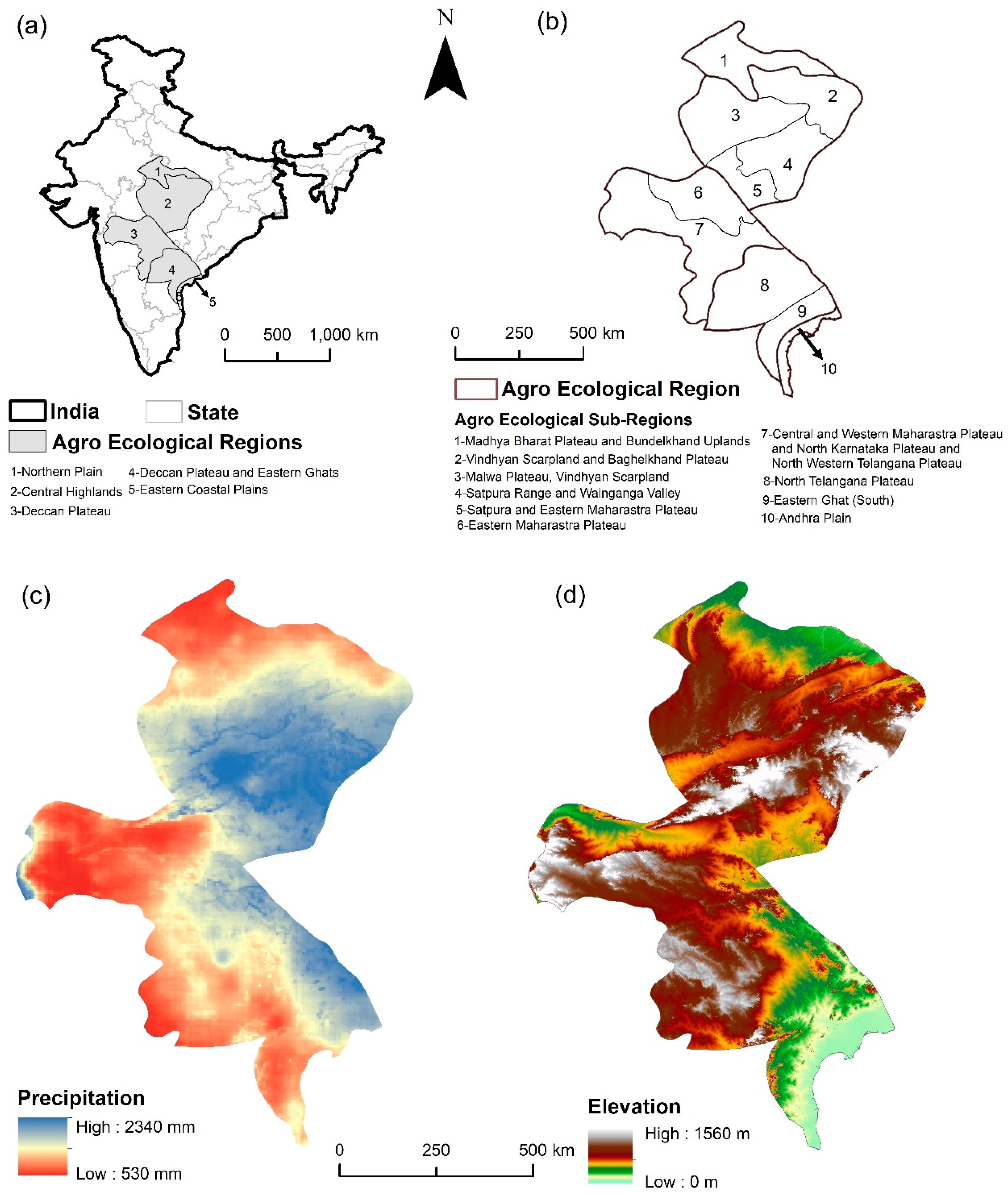
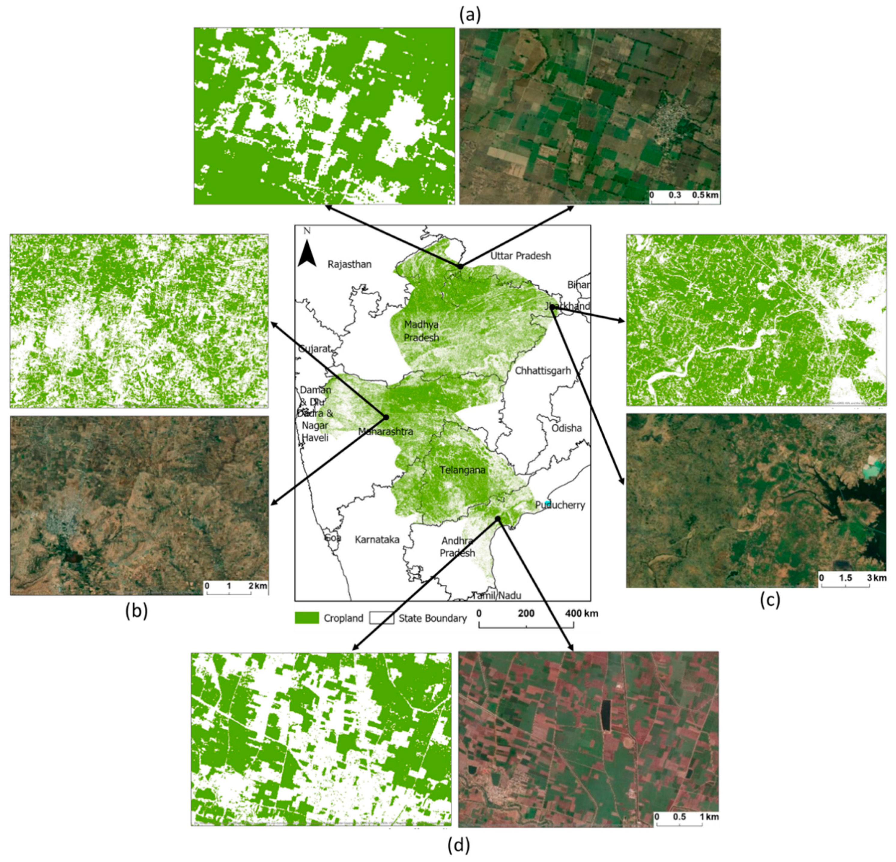
The study area comprises of ten sub-regions within five agro-ecological regions (AER) covering the Indian states of Uttar Pradesh, Madhya Pradesh, Chhattisgarh, Maharashtra, Andhra Pradesh, and Karnataka (Figure 1) [58]. The study area covers approximately 604,615 km2 and is surrounded by the alluvial Gangetic plains in the north and the Bay of Bengal in the south. It borders the Western Ghats in the west and Chota Nagpur plateau in the east. The region is mostly undulating with the elevation ranging between 0–1560 m (Figure 1).
The region has a tropical monsoon climate (Am) as per the Koppen-Geiger climate classification system [59]. The mean annual rainfall ranges approximately from 530 mm to 2300 mm across the region (Figure 1c), as calculated from the Climate Hazards Group InfraRed Precipitation with Station (CHIRPS) data for 2000–2018. Most of the farmers in the study region are smallholders with limited landholdings; they grow crops during three seasons: monsoon (kharif) during June-November, winter (rabi) during December-April, and summer (zaid) during April–June [60]. The major monsoon crops grown in the study region are rice, soybean, black gram (locally known as Urad), cotton, maize, and groundnut [61]. The monsoon crop sowing date varies across the study region, starting in the month of June with the onset of monsoon, up to August/September in low-lying regions. The harvesting of the crops widely varies as well and may range from September for soybean and black gram to November for rice. The details regarding the AERs considered for this study and the major monsoon crops grown according to the latest government statistics available are listed in Table 1 [61]. For further analysis, we have combined AER-5 with AER-4, as AER-5 has negligible cropped area to be analyzed as separate unit. Diverse monsoon crops are grown in the AERs comprising of both water intensive monsoon crops and rainfed-dryland crops.
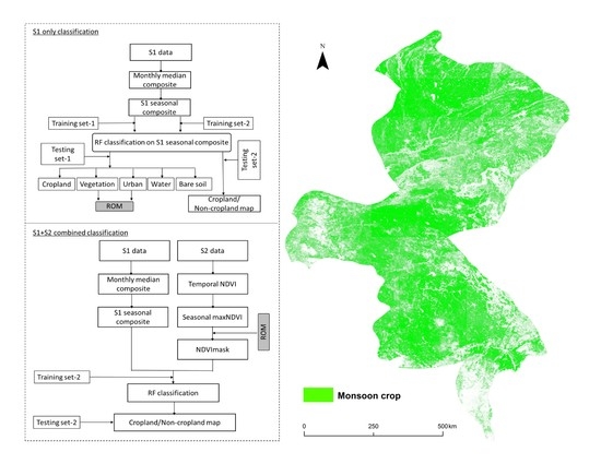
2.2. Overall Workflow
The flowchart for the methods used in this study is outlined in Figure 2. In the first step, S1 and S2 time series images were loaded on Google Earth Engine (GEE) platform using ‘ImageCollection’ function [62]. These images were then filtered based on time (June–November 2018) and study region boundary. For S1 SAR, we used images from June to November, but for S2 optical data, we considered images from July to November. The month of June was not considered for S2 optical data as summer crops were still at their peak growth stage in some regions and the land preparation and sowing of monsoon crops were in the initial stages. A ‘cropped field’ in June would thus be an indication of summer crops, and not monsoon crops. Further image classification was performed on S1 (Figure 2b), and S1+S2 combined (Figure 2c), using pixel-based machine learning classifier (random forest) on GEE. We have used pixel-based classifier instead of object-based classifier for large monsoon cropland mapping, as the latter requires high computation time and has complicated intermediate steps including the segmentation where specific parameter tuning is needed [32,63,64]. Even though object-based classifiers might improve the classification accuracy in some landscapes, this performance improvement is not always evident in complex heterogeneous landscapes such as the one showed in this study. We further performed accuracy assessments for the four AERs (Table 1). Training and testing of the classified images were performed according to the procedure detailed in Figure 2a and Section 2.2.2.
2.2.1. Satellite Data Pre-Preprocessing
We used freely available S1 SAR data and S2 optical data provided by the European Space Agency (ESA) and images were accessed and processed on the GEE platform [65]. We used S1, C-band, dual-polarization VV (single co-polarization, vertical transmit/vertical receive) and VH (dual-band cross-polarization, vertical transmit/horizontal receive) dataset for the Interferometric Wide Swath (IWS) mode in the descending look angle [66]. The GEE platform provides S1 data pre-processed with thermal noise removal, radiometric calibration and ortho-rectification using the Sentinel-1 toolbox resulting in ground-range detected images with backscattering coefficients in decibel (dB) scale.
Using temporal VH and VV polarization, SAR monthly composite images were created by considering median values. We also used these monthly median composite images to create False Color Composite (FCC) to aid in visual interpretation of the images for training and testing data collection (Figure 4). For optical data, we used the S2 level 1-C, ortho-rectified and geo-referenced top-of-atmosphere (TOA) reflectance data product [67]. The collection contains Multi Spectral Instrument (MSI) bands with a scaling factor of 10,000. To maintain the quality of the data analysis and products during the monsoon season, we considered Sentinel-2 images with cloud cover of 5% or less. On these filtered images, we applied an automated cloud masking algorithm using quality assessment band (band QA60) to mask both opaque and cirrus clouds [68]. The images acquired after the month of November were not considered as we assumed that crops grown after this time are not monsoon crops, based on existing literature [24,60]. A total of 516 S1 images and 1734 S2 images were used for the entire monsoon crop-growing season of 2018.
2.2.2. SAR Temporal Backscattering
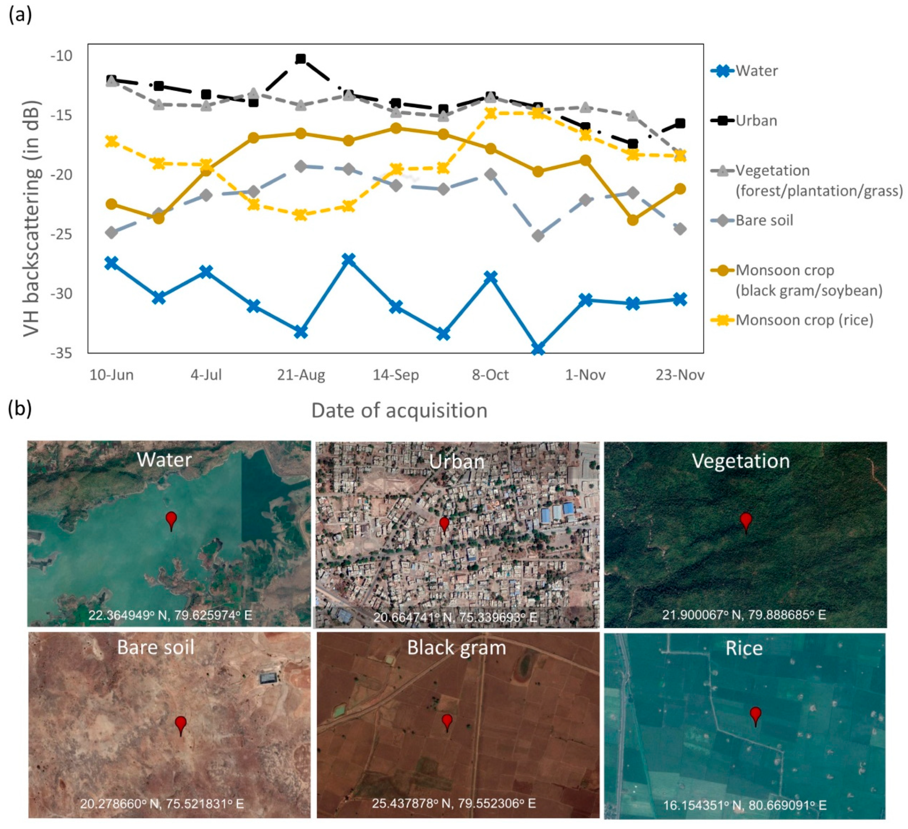
Temporal backscattering profiles were obtained using C-band VH polarization S1 imagery from monsoon crops (rice and black gram/soybean), bare soil, urban, water and vegetation (forest/plantation/grass) features shown in Figure 3a, similar to what obtained by Singha et al. [31]. The backscattering profiles were generated by taking the mean of 10 sample points for each class spread across the study area. The sample points for each class along with their geolocations are shown in Figure 3b.
Vegetation is defined as land surface with plants and includes plantation, grass and forest. The contrasting nature of backscattering from vegetation and monsoon crops forms our basis of utilizing the temporal S1 backscattering signatures for Radar Optical cross Masking (ROM) as discussed in Section 2.2.6 below. As displayed in Figure 3a, temporal SAR backscattering signatures are effective in separating crops (rice, black gram, and soybean) from water, urban and vegetation. However, these signatures are mixed with bare soil during the crop-growing season. So, it becomes difficult to segregate crops from bare soil with very high accuracy using only S1 SAR data. Hindrance in segregating crops from bare soil forms our basis of integrating optical data with SAR as bare soil is very distinct in optical data compared to crops and other vegetation due to its lack of ‘greenness’ reflected in low Normalized Difference Vegetation Index (NDVI) values [69].
In the study region, the SAR backscattering signatures obtained from vegetation (forest/plantation/grass) and urban class are non-dynamic throughout the monsoon season, and have nearly constant high backscattering values (~−16 dB to −10 dB) compared to other LULC features. During the time of classification, there is high probability of vegetation class being mixed with urban and vice versa. Monsoon crops and bare soil have dynamic backscattering throughout the crop growing season. For crops such as black gram and soybean, the land preparation starts from first week of June and last until mid-July based on the onset of the monsoon. For these monsoon crops, the backscattering is initially low due to land preparation in June and increases with time as the crop grows. For rice, land preparation starts in the July/August when the fields have sufficient amount of water as rice is a water intensive crop [31]. Rice shows very low backscattering during the land preparation/transplanting stage. During the time of maturity, the backscattering increases for both black gram/soybean and rice. The backscattering is high for rice compared to black gram/soybean due to high biomass content resulting in high volume scattering from the rice fields.
For bare soil, the initial backscattering is similar to that obtained from black gram/soybean due to the presence of exposed soil with no crop cover. It can be seen that bare soil signature can get mixed with that from rice in the month of July. Hence, overall it is very difficult to segregate monsoon crops from bare soil with very high accuracy. For water, the backscattering is very low (<−25 dB) throughout the monsoon season, hence it is easily segregated from monsoon crops.
2.2.3. Training and Testing the Classifiers
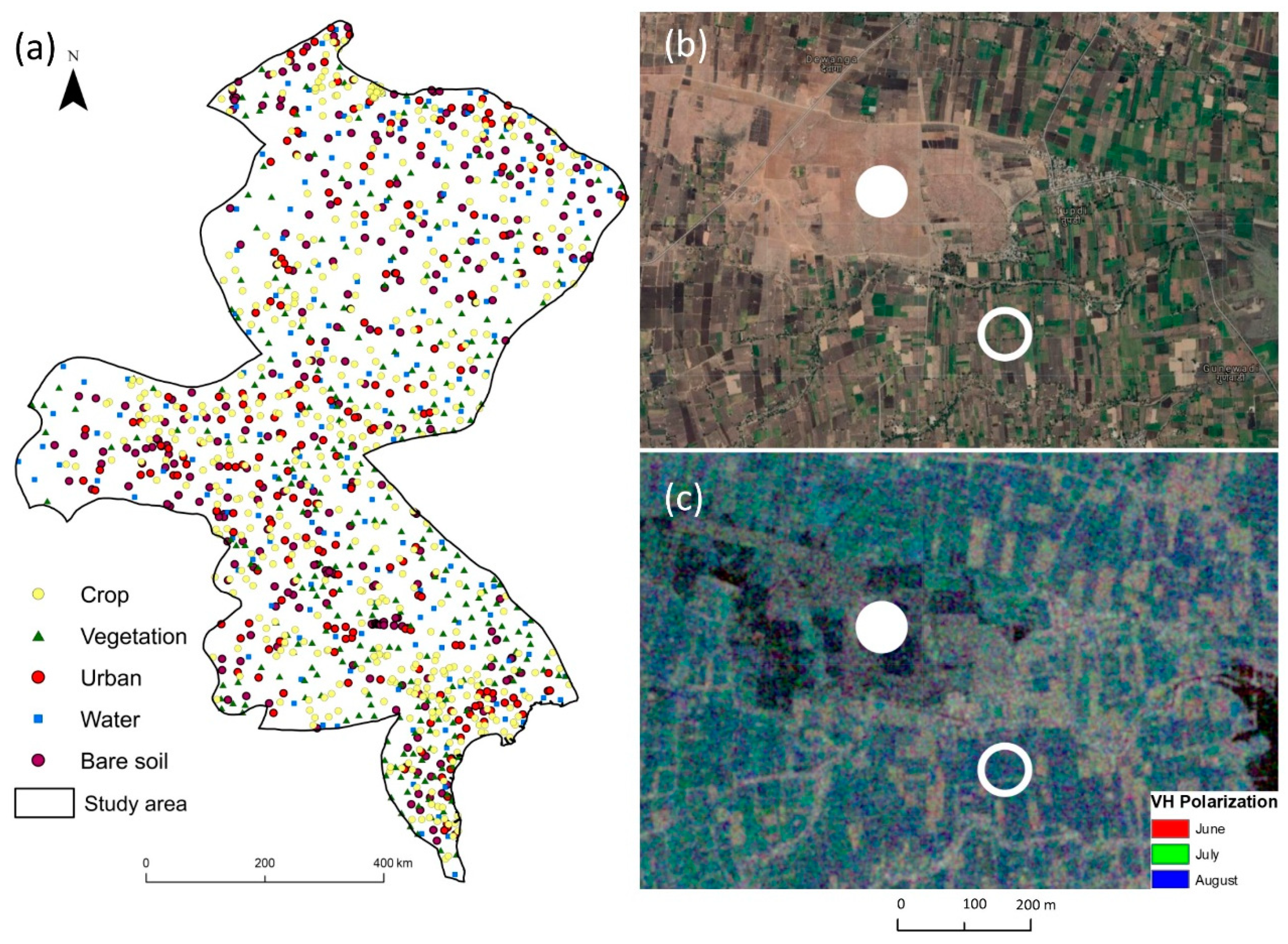
We collected a total of 1500 reference points required for training and testing the classifiers for the five broad land use land cover (LULC) classes: monsoon crop, bare soil, water, vegetation, and urban (Figure 4a). We defined bare soil as any land cover feature, which is devoid of vegetation, either a barren land, fallow land with no crop, or any region with exposed soil. We collected these points through a combination of field visits, high-resolution google earth imagery and visual interpretation of S1 and S2 satellite imagery using the method similar to those explained in [31,70]. Using multiple datasets to generate the training and testing points ensures that only land cover features, which have the high probability of belonging to the actual land cover class on the ground, are selected for training and testing. During field visits, information on land covers along with their geographic coordinates were collected using a handheld Global Positioning System (GPS) device. Field visits were conducted at four agro-ecological sub-regions: (1) Madhya Bharat Plateau and Bundelkhand Uplands, (2) Vindhyan Scarpland and Baghelkhand Plateau, (3) Eastern Ghats (South), and (4) Andhra Plain (Figure 1b). We collected a total of 500 points for monsoon crops, 300 points each for bare soil and vegetation, and 200 points each for water and urban, using stratified random sampling approach. The number of points collected for each land cover was decided based on the relative dominance of these land covers in the study landscape.
First, the field data points were imported on GEE platform and were overlaid on the S1 and S2 FCC images. Using this ground truth data, the extracted features were used to identify similar LULC features in other regions using visual interpretation techniques on FCC of S1 and S2. The extracted features were verified using the high-resolution google earth imagery. Extracting training points for water, forest/plantation and urban is straightforward in S1 as they are not dynamic over time and have very distinct temporal backscattering signatures compared to crops and bare soil as shown in Figure 3 and explained in Section 2.2.2. We only assigned a reference point to a particular LULC, if the corresponding LULC class was confirmed in all three layers (S1 FCC, S2 FCC, and high-resolution google earth imagery). Finally, the field data points and points generated through visual interpretation were merged together to be used for training and testing on GEE platform (Figure 4a). Representative reference points for monsoon crop and bare soil are shown in Figure 4b,c. We randomly identified 70% of the 1500 reference points as ‘training points’ using the ‘randomColumn’ function in GEE and used those for training the random forest (RF) classifier. The rest of the reference points (30%) was used as ‘testing points’, i.e., for post-classification accuracy assessment. To avoid any biases in selecting the training and testing points, we performed the classification and accuracy assessment iteratively for 20 times by randomly dividing training and testing points in 70:30 ratio.
2.2.4. Classification Based on Sentinel-1
We considered a monthly composite of SAR data using both VH and VV (VH + VV) polarization, instead of a single date image for S1 classification, as previous studies have shown that multi-temporal SAR data perform far better than single SAR image for crop classification [41,45,47]. Considering multi-temporal SAR data becomes even more important for diversified cropping pattern in India as such data are able to take into account the variation of crops grown in different time of the season. Using the training dataset, the RF classifier was run on monthly median composite of June–November 2018. The RF is an ensemble classifier that follows the decision tree approach in which randomly selected results from multiple decision trees are combined together to obtain highly accurate and stable classification results [65,66,67,68]. RF algorithm can handle large quantity of complex multi-source data and is robust against overfitting. For initiating RF classifier, the user must define two parameters, the number of trees to grow and the number of variables used to split each node. In this work, the number of decision trees used are 100 and the variables used to split each node was set to square root of the number of overall variables. Previous studies have shown that RF classifier outperforms other parametric classifiers such as Support Vector Machine (SVM) in obtaining improved classification results [71,72,73,74]. RF outperforms SVM in many ways as it can handle large database of temporal images, requires less training time. In addition, the number of user-defined parameters required in RF are less and easier to define compared to SVM [75,76,77]. RF performs better if there are sufficient amount of training dataset as we have in this study. RF is also successful in discriminating classes with similar characteristics such as crops and vegetation [78]. For this study, S1-based classification was performed using two different output criteria: one with a classified map with five classes (Section 2.2.3) and the other with only two classes – cropland and non-cropland (obtained by combining non-cropland classes, i.e., bare soil, water, vegetation and urban). In addition, we calculated the classification accuracy for each AER separately. The classification and accuracy assessments were performed 20 times using unique set of training and testing data.
2.2.5. Seasonal Normalized Difference Vegetation Index (NDVI)
The Normalized Difference Vegetation Index (NDVI) is a widely used remote sensing measure to assess the health of the vegetation and to differentiate crops, and other vegetation (forest, plantation, grass) from bare soil, water and urban [79]. NDVI is a unitless measure and ranges between −1 and 1. Healthy vegetation typically has higher NDVI values compared to non-vegetated surfaces. For calculating NDVI, we require the red and near-infrared (NIR) reflectance bands (Equation (1)):
NDVI = (NIR − Red)/(NIR + Red)
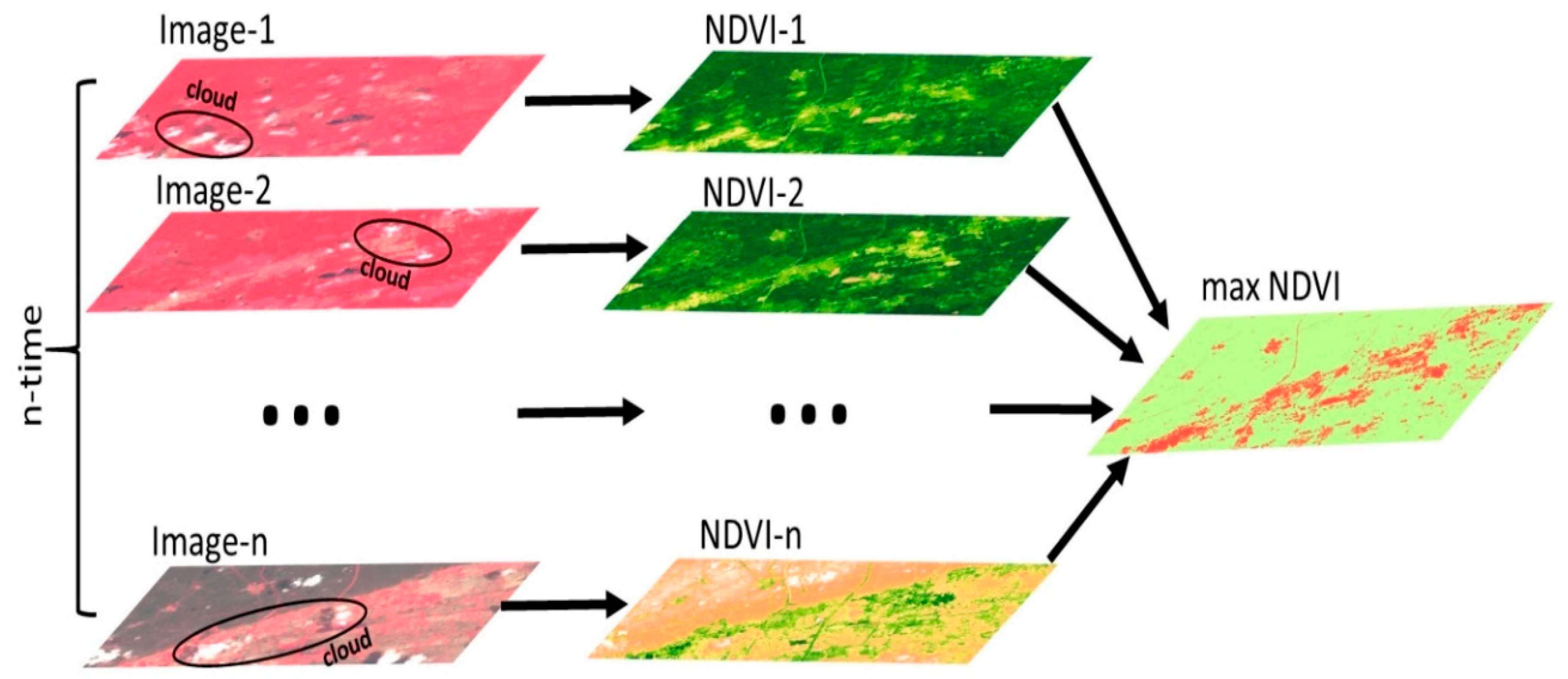
In S2 imagery, we used band 4 and band 8, respectively, for red and NIR in the above equation. We calculated NDVI for all the available cloud free pixels in our image as our main focus was on cropped field identification, especially since previous studies have shown high correlation between NDVI and photosynthetic activities of the cropped fields [80]. To generate the seasonal maximum value of NDVI (maxNDVI), we performed temporal aggregation of NDVI from July to November (Figure 5). Temporal aggregation is an approach to perform pixel-based analysis over a period of time using metrics (i.e., mean, median, maximum etc.) from satellite derived reflectance or satellite-derived indices (e.g., NDVI, Enhanced Vegetation Index (EVI), etc.) [68]. The aggregation addresses the problem of lack of continuity in the optical data due to cloud cover and reduces the volume of data for further processing [68,81]. During monsoon season, optical satellite images in India contain considerable amount of cloud patches, which affects the radiometric quality of the images, thus limiting intra-seasonal crop monitoring capability. We calculated maxNDVI in order to fill this data gap and to capture the crop heterogeneity, i.e., considering all monsoon crops with different intra-seasonal phenology. In this maxNDVI dataset, both crops and vegetation (forest/plantation) have higher values compared to water, urban and bare soil. We further utilized the Otsu’s thresholding approach in GEE, to differentiate between the crops/vegetation (forest, plantation) from non-vegetative features with low NDVI values (bare soil, urban and water) [82]. This approach is an automated way of finding an optimal global threshold based on the observed distribution of pixel values. Based on the pixel value distributions for the LULC classes considered in this study, the Otsu’s thresholding value for maxNDVI is 0.36.
2.2.6. Radar Optical cross Masking (ROM)
It was not possible to differentiate between crop and vegetation within the maxNDVI dataset, which is an important step for a crop mapping procedure involving optical data. Due to non-availability of high-resolution (10m) non-crop mask for the region, we developed a method of masking non-crop vegetation from maxNDVI using classified SAR imagery (Figure 2b). From the S1-derived classified map with five LULC classes, vegetation (forest/plantation/grass) and urban classes were further combined together as a non-dynamic class to obtain the non-crop mask and to segregate crops from vegetation in maxNDVI imagery. We combined vegetation and urban as one class, instead of considering only vegetation, since these two classes have similar backscattering signatures and are difficult to segregate in S1-derived map as described previously (Section 2.2.2, Figure 3). Moreover, combining urban and vegetation to obtain the non-crop mask is less likely to affect our outputs, as urban class is already masked out from the maxNDVI data due to the application of Otsu’s thresholding. We coined this technique as Radar Optical cross Masking (ROM) where we used the non-dynamic, non-crop (urban + vegetation) mask to separate vegetation from crops resulting in crop only maxNDVI dataset (NDVImask; Figure 2c).
2.2.7. Classification Based on Combined Sentinel-1 and Sentinel-2
In this step, the S1 data and NDVImask were combined for pixel-based classification to examine if adding NDVImask imagery will result in improved monsoon crop mapping accuracy compared to using S1 only classified map. Combining S1 and NDVImask will also address some of the limitations of using only S1 data for monsoon crop mapping (Section 2.2.2, Figure 3). The monthly median SAR composites from June to November were stacked together with NDVImask data obtained after using ROM. The RF classifier was run on the combined dataset with the number of trees set as 100 and the variables to split each node set to square root of the number of overall variables. The output from this classification is a binary crop/non-crop map using training and testing set-2 (Figure 2c). Similar to the S1-based classification, the combined S1 and S2-based classification and accuracy assessment were repeated for 20 times to avoid any biases in the classification accuracy.
2.2.8. Accuracy Assessment
Both classification outputs obtained from S1 and combined S1 and S2 were evaluated and compared using the standard count-based accuracy assessment methods of overall accuracy (OA) and kappa coefficients obtained from the confusion matrix [83] using 20 different iterations. User’s accuracy (UA) and producer’s accuracy (PA) were calculated using 30% testing points that were not involved in training the classifiers. UA measures the error of commission, i.e., the proportion of pixels that were incorrectly included in a class that is being evaluated. PA measures the error of omission, i.e., the proportion of pixels in a certain class that is being evaluated that were incorrectly classified in another category, and were omitted from the ‘truth’ class as identified by the test points.
We further calculated the F-score to determine the degree of discrimination among the five LULC classes obtained from the S1-derived classification and the binary crop vs non-crop classification obtained from S1 only and S1+S2 combined derived classification. The F-score ranges between 0 and 1, with higher values denoting better discriminating power among the classes. The F-score is calculated using Equation (2) mentioned below [84]:
We did not compare the accuracy of the results obtained with the crop estimates provided by government due to non-availability of crop census data for the monsoon crop season 2018–2019.
3. Results
3.1. Accuracy of S1 Only Classification
The classification accuracy obtained from S1-derived classification using training and testing set-1 is shown in Table 2. The OA obtained after 20 iterations is 80.0%. The kappa coefficient obtained is 0.74 (Table 2). Our results indicate that the water class was easily identified (F-score = 0.96) using SAR data among the five LULC classes. The low F-score obtained for urban (0.64) class indicates that the S1 SAR data has the least discriminative capability to segregate urban from other classes. SAR data was moderately successful in discriminating monsoon crops from other land cover classes (F-score = 0.84).
3.2. Accuracy of Binary Crop Maps from S1 Only and Combined S1 and S2
The comparison of accuracy assessment obtained from S1 only and S1+S2 combination using training and testing data set-2 is displayed in Table 3. The crop vs. non-crop overall classification accuracy obtained by S1+S2 combination is approximately 3% higher than obtained by using S1 only dataset. The standard deviation of kappa values while randomly changing the training and testing points for 20 classifier iterations are slightly higher for S1 only compared to S1+S2 classification. The F-score for both S1 and S1+S2 classification shows high discriminative capability (>0.85). Moreover, the F-score for the combined S1+S2 is higher compared to S1 only classification for both crop and non-crop class.
NDVImask image obtained after applying ROM on maxNDVI is shown in Figure 6. It can be seen that non-dynamic forest/plantation regions can be effectively separated from crops using ROM. In the figure, regions with forest and plantation (casuarina and eucalyptus) are masked out using ROM to obtain NDVImask image with crops only. The crop map generated using combined S1 and S2 data is shown in Figure 7. Detailed zoom-in views for selected locations using the combined S1+S2 classification and its comparison with high-resolution imagery are also shown (Figure 8). It can be observed that the combined approach is efficient in differentiating monsoon cropland from plantation (such as mentha/casuarina/eucalyptus) in AER-1 (Figure 8a) and AER-4 (Figure 8c).
3.3. Accuracy of Binary Crop Maps for Each AER
The comparison of accuracy assessments obtained from S1 only and S1+S2 combination using training and testing data set-2 for the selected AER regions are shown in the Table 4. We found that for all of the AERs, OA obtained from S1+S2 combination outperformed the one obtained from S1 only classification and the improvement varies across the AERs. Also, the OA obtained by the combined S1+S2 was greater than 90% for all of the AERs. The OA difference between S1+S2 and S1 was the lowest for the AER-3 (Table 4), whereas it was greater than 4% for the other three selected AERs. For AER-1, which is dominated by rainfed-dryland crops (90%) with some rice-growing regions (10%), there is a 4% improvement in classification accuracy from S1 to S1+S2. For the S1 dataset, low classification accuracy of AER-2 and AER-4 and 5 compared to the other two AERs is due to the fact that these two regions are dominated by vegetation mixed with crops and have hilly undulating terrain which may have reduced the S1 classification accuracy. AER-2 hosts Vindhyachal and Satpura range whereas AER-4 and 5 are dominated by Eastern Ghats and fragmented vegetation. For both these regions, classification accuracy improved by 5% when S1 data is combined with S2 data. In addition, late maturity crops such as rice or cotton dominate these two regions. Hence, contribution from S2 data towards classification accuracy increases in these regions with increasing availability of cloud free optical data towards the end of the monsoon season. For AER-3, it was observed that combined S1+S2 dataset shows no major improvement over S1 only classification. This region is mainly a plateau with less variation in elevation and negligible forested land. Hence the mixing of crops with natural vegetation is limited resulting in no major inaccuracy in S1-derived classification due to terrain or vegetation.
4. Discussion
4.1. Monsoon Crop Mapping by Combining S1 and NDVImask
Due to the lack of free time-series of SAR data until recently, previous studies mostly focused on using medium resolution Landsat data (30 m) or MO DIS data (250 m) over large geographic region for monsoon cropland mapping [20,21,22,23,24,25,26,27]. However, using MODIS or Landsat might not be the best approach for monsoon cropland mapping due to frequent cloud cover [24,26]. The spatial resolution of these coarse resolution satellites is not suitable either to capture the small field sizes or mixed agriculture landscapes, thus limiting their usage for preliminary assessment and understanding of croplands over large region. Relying on cloud free optical data alone is not always viable for studying monsoon crops as most of the crops are harvested before cloud free scenes become available in the late monsoon season. Using SAR data during the monsoon season can address this issue. However, SAR data suffers from speckle effects, which makes it difficult to use SAR data alone for generating reliable crop statistics across large regions [65]. Both optical and SAR sensors have limitations for monsoon crop study, but a synergistic approach of combining these data can improve the crop mapping for small-scale farmers at high resolution (Figure 7 and Figure 8). The technique used in this study differ from other published literature as we propose a new way of pixel-based combination of SAR data with temporal aggregation of optical data (maxNDVI) using ROM. Previous studies for monsoon crop monitoring using combination of SAR and optical data were limited to water-intensive rice crops and/or small geographic regions where it was possible to obtain at least one cloud free optical image [34,53,57]. The results presented in this work are important, as this will provide the first high-resolution (10 m) monsoon cropland map generation, and can also be transferred to other agro-ecoregions. This method shows an improvement over existing methods that are primarily focused on non-monsoon/winter cropland mapping at 30 m or coarse resolution [20,24,27,85].
Several sources of error might have affected the results from the S1+S2 combined methodology presented in this study. One of the reasons may be due to the lack of cloud free S2 pixels during the crop growing season. It is possible that in some regions the classification results were solely generated from SAR data due to the non-availability of a single cloud-free S2 image, and could result in inconsistencies in accuracy. There might be errors while training the model and/or due to mixed pixels which may reduce the classification accuracy. The study area is complex with varying farming practices which may result in misclassification of land cover classes in SAR data. Also, the variations in SAR backscattering due to geometric errors (layover, shadow) over hilly terrain affects the accuracy [31]. Using temporal SAR data, along with stratified random sampling and running multiple iterations of the RF classifier reduces the biases, however doesn’t completely eliminate it. Using the automatic Otsu thresholding method to extract vegetation cover and segregate vegetation from low NDVI values representing soil, water, and other non-vegetated regions in optical data reduces the overall uncertainty as well.
The ROM generated from S1 SAR data, addresses the issue of miss-classification of spectrally similar plantation and forested vegetation with monsoon crops as visually interpreted (Figure 6). During the monsoon season, optical datasets are only available towards the end of season when crops have already been harvested or are in their peak growth stages [26]. During the peak-growth stage, the spectral signatures of these crops are similar to plantation or other non-crop vegetation, thus making it difficult to segregate the monsoon crops from natural vegetation [31,32,33]. The usage of temporal SAR-based phenology to generate five land cover classes to produce ROM, masks out the vegetation from monsoon cropland, and improves the classification accuracy (Figure 6 and Figure 8). ROM helps in segregating monsoon cropland from plantation and natural vegetation (forest/grassland) and can be utilized for large regions, as it is not affected by clouds. The ROM produced here is dynamic and can be regularly updated based on the available SAR images. The ROM may also have applications in LULC change monitoring and segregation of non-dynamic LULC features from dynamic croplands.
Overall, our method of integrating SAR composite with seasonal NDVImask for monsoon cropland mapping overcomes four main challenges of mapping smallholder agriculture across large spatio-temporal scales: (i) the method works well in different agro-ecological regions as it takes into consideration of the crop planting time and duration, (ii) it can be used in regions with high cloud cover, such as most tropical countries, (iii) it reduces the sub-pixel heterogeneity in mapping monsoon cropland as the resolution of the output cropland map (10 m) better matches the small farm sizes in most developing countries, and (iv) it helps in distinguishing between monsoon cropland areas from plantation/natural vegetation which has similar signatures during the peak crop growing season. The high-resolution monsoon cropland map produced in this work has the potential to assist government agencies, landscape managers, and researchers in monitoring monsoon crops, which in turn would help us to better understand the factors influencing the production of these crops. Until now, it takes more than a year to make these crop estimates available for decision makers and researchers. This study also has the potential to support global agriculture monitoring missions of Sen2Agri and Geo Global Agriculture Monitoring (GEOGLAM). The objective of GEOGLAM is to provide timely, easily accessible scientifically validated remotely sensed data and derived products for crop-condition monitoring and production assessment. Also, one of the requirements of Sen2Agri mission is to produce national scale dynamic cropland masks other than producing cloud free composites, crop type maps and to indicate the status of current vegetation at 10 m resolution [27,86]. Previous research conducted for Sen2Agri mission to generate dynamic cropland was limited in scope in tropical regions as they relied only on optical datasets [86,87]. This work supports the GEOGLAM and Sen2Agri mission as it produces high-resolution monsoon cropland map over large region comprised of different crop-growing regions. The methodology developed here is also suitable for generating national level dynamic cropland masks.
4.2. ROM Uncertainty
In this study, S1-based classification was performed using the RF classifier and training and testing data set-1 for generating ROM. The accuracy of ROM and in turn NDVImask depends on how accurately the non-dynamic land use/cover classes are classified. Based on the classification accuracy (Table 2), it was observed that PA was lowest for the urban class. There were many instances where urban area on the ground was misclassified as other classes including vegetation, likely due to the presence of tree canopy cover in urban centers. The accuracy of ROM will vary depending on whether these omitted ‘urban’ points are being classified as ‘vegetation’ or other classes. Our results indicate that UA was the lowest for vegetation class (Table 2) which shows that points from other classes were committed to the vegetation class. The overall accuracy of the classification will also affect the performance of ROM. The F-scores for urban (0.64) and vegetation (0.71) show low discriminative capability compared to the water (0.96) and monsoon crop (0.84) classes (Table 2). Thus, this may also have affected the accuracy of ROM. Visual inspection of the output maps revealed that the classification accuracy of S1 data to obtain ROM was high for plantation compared to forested regions (Figure 6c–f). This is due to the fact that in our study region, forested regions are mainly found in hilly and mountainous regions, which are affected by geometric errors such as layover or shadow and thus affect the classification accuracy. Also, the forested regions in this part of India is either open forest or scrubland which has open spaces or bare soil in between the canopies, affecting the accuracy of ROM [88].
To improve the classification accuracy of S1 for ROM generation, second order texture measures, which involves using Grey-Level Co-occurrence Matrices (GLCM), can be included for improving the classification accuracy of SAR data, especially for discriminating forest and plantation regions [53]. In addition, with advancement in technology and availability of large amount of satellite data, more powerful deep learning methods such as long short-term memory (LSTM), which efficiently handles time series data, may be utilized for improving the overall classification accuracy and in producing ROM in particular [89,90].
5. Conclusions
This study presents a synergistic approach of combining SAR with optical data for monsoon crops over different agro-ecological regions in India utilizing the GEE platform. The overall accuracy of 93%, for the binary cropland/non-cropland map, suggests that the combined approach introduced in this research is reliable for monsoon cropland mapping, especially in regions dominated by rainfed-dryland crops. The combined approach provides classification accuracy of 90% or more in different agro-ecological regions dominated by diverse crops. The ROM proposed here has overcome the challenge of differentiating natural vegetation from monsoon cropland mapped during the peak growth stages in monsoon season. Thus, it has applications for segregating cropland from vegetation cover, and may assist in generating a non-crop mask in regions affected by cloud cover. This study can provide important information for decision makers and researchers as monitoring these crops is a challenging task due to small farm size and frequent cloud cover during the crop-growing season.
Author Contributions
Conceptualization, A.Q. and P.M.; methodology, A.Q.; writing—original draft preparation, A.Q.; writing—review and editing, P.M.; funding acquisition, P.M. All authors have read and agreed to the published version of the manuscript.
Funding
This research was funded by the University of Delaware Research Fund awarded to P.M.
Acknowledgments
The authors would like to acknowledge four anonymous reviewers for their constructive feedback on the earlier version of this manuscript. The authors are thankful to Delphis Levia (University of Delaware) and Rodrigo Vargas (University of Delaware) for their constructive feedback and intellectual support during this research work, and to the Department of Geography and Spatial Sciences (University of Delaware) for supporting Open Access Publishing by funding the article processing charge. The authors are grateful to the officials of District Agriculture Department of Uttar Pradesh, Madhya Pradesh, Andhra Pradesh, the scientists of Acharya N G Ranga Agricultural University, Guntur and Touseef Ahmed (Acharya Nagarjuna University College of Engineering and Technology) for their assistance and co-operation during the field surveys. The authors appreciate constant support of Meghavi Prashnani (University of Maryland) and Matthew Walter (University of Delaware) during this research.
Conflicts of Interest
The authors declare no conflict of interest.
References
- Madhusudhan, L. Agriculture Role on Indian Economy. Bus. Econ. J. 2015, 6, 1. [Google Scholar]
- Gadgil, S.; Gadgil, S. The Indian monsoon, GDP and agriculture. Econ. Political Wkly. 2006, 41, 4887–4895. [Google Scholar]
- Gadgil, S.; Rupa Kumar, K. The Asian monsoon—Agriculture and economy. In The Asian Monsoon; Springer: Berlin/Heidelberg, Germany, 2006; pp. 651–683. [Google Scholar]
- Krishna Kumar, K.; Rupa Kumar, K.; Ashrit, R.G.; Deshpande, N.R.; Hansen, J.W. Climate impacts on Indian agriculture. Int. J. Climatol. 2004, 24, 1375–1393. [Google Scholar] [CrossRef]
- Fritz, S.; See, L.; Bayas, J.C.L.; Waldner, F.; Jacques, D.; Becker-Reshef, I.; Whitcraft, A.; Baruth, B.; Bonifacio, R.; Crutchfield, J.; et al. A comparison of global agricultural monitoring systems and current gaps. Agric. Syst. 2019, 168, 258–272. [Google Scholar] [CrossRef]
- Ramaswami, B.; Ravi, S.; Chopra, S.D. Risk management in agriculture. In Discussion Papers; Indian Statistical Institute: Delhi unit, India, 2003. [Google Scholar]
- Venkateswarlu, B.; Prasad, J. Carrying capacity of Indian agriculture: Issues related to rainfed agriculture. Curr. Sci. 2012, 102, 882–888. [Google Scholar]
- Suresh, A.; Raju, S.S.; Chauhan, S.; Chaudhary, K.R. Rainfed agriculture in India: An analysis of performance and implications. Indian J. Agric. Sci. 2014, 84, 1415–1422. [Google Scholar]
- Srinivasarao, C.; Venkateswarlu, B.; Lal, R.; Singh, A.K.; Kundu, S. Sustainable management of soils of dryland ecosystems of india for enhancing agronomic productivity and sequestering carbon. In Advances in Agronomy; Academic Press Inc.: Cambridge, MA, USA, 2013; Volume 121, pp. 253–329. [Google Scholar]
- Department of Agriculture Cooperation and Farmers Welfare, Government of India. Annual Report. Available online: http://agricoop.nic.in/annual-report (accessed on 30 August 2019).
- Division, A.I. District Wise Land Use Statistics. Available online: http://aps.dac.gov.in/APY/Index.htm (accessed on 30 August 2019).
- Craig, M.; Atkinson, D. A Literature Review of Crop Area Estimation; UN-FAO Report. 2013. Available online: http://www.fao.org/fileadmin/templates/ess/documents/meetings_and_workshops/GS_SAC_2013/Improving_methods_for_crops_estimates/Crop_Area_Estimation_Lit_review.pdf (accessed on 20 October 2019).
- Laamrani, A.; Pardo Lara, R.; Berg, A.A.; Branson, D.; Joosse, P. Using a Mobile Device “App” and Proximal Remote Sensing Technologies to Assess Soil Cover Fractions on Agricultural Fields. Sensors 2018, 18, 708. [Google Scholar] [CrossRef] [Green Version]
- Strengthening Agricultural Support Services for Small Farmers, Report of the APO Seminar on Strengthening Agricultural Support Services for Small Farmers Held in Japan. 2001. Available online: https://www.apo-tokyo.org/publications/wp-content/uploads/sites/5/pjrep-sem-28-01.pdf (accessed on 30 August 2019).
- Dadhwal, V.K.; Singh, R.P.; Dutta, S.; Parihar, J.S. Remote sensing based crop inventory: A review of Indian experience. Trop. Ecol. 2002, 43, 107–122. [Google Scholar]
- Parihar, J.S.; Oza, M.P. FASAL: An integrated approach for crop assessment and production forecasting. In Agriculture and Hydrology Applications of Remote Sensing, Proceedings of the SPIE Asia-Pacific Remote Sensing, Goa, India, 13–17 November 2006; Kuligowski, R.J., Parihar, J.S., Saito, G., Eds.; SPIE: Bellingham, WA, USA, 2006; Volume 6411, p. 641101. [Google Scholar]
- Deschamps, B.; McNairn, H.; Shang, J.; Jiao, X. Towards operational radar-only crop type classification: Comparison of a traditional decision tree with a random forest classifier. Can. J. Remote Sens. 2012, 38, 60–68. [Google Scholar] [CrossRef]
- Shanahan, J. Use of Remote-Sensing Imagery to Estimate Corn Grain Yield Agronomy—Faculty Publications Use of Remote-Sensing Imagery to Estimate Corn Grain Yield. Agron. J. 2001, 93, 583–589. [Google Scholar] [CrossRef] [Green Version]
- Jones, J.W.; Antle, J.M.; Basso, B.; Boote, K.J.; Conant, R.T.; Foster, I.; Godfray, H.C.J.; Herrero, M.; Howitt, R.E.; Janssen, S.; et al. Toward a new generation of agricultural system data, models, and knowledge products: State of agricultural systems science. Agric. Syst. 2017, 155, 269–288. [Google Scholar] [CrossRef] [PubMed]
- Pittman, K.; Hansen, M.C.; Becker-Reshef, I.; Potapov, P.V.; Justice, C.O. Estimating global cropland extent with multi-year MODIS data. Remote Sens. 2010, 2, 1844–1863. [Google Scholar] [CrossRef] [Green Version]
- Granados-Ramírez, R.; Reyna-Trujillo, T.; Gómez-Rodríguez, G.; Soria-Ruiz, J. Analysis of NOAA-AVHRR-NDVI images for crops monitoring. Int. J. Remote Sens. 2004, 25, 1615–1627. [Google Scholar] [CrossRef]
- Jiang, D.; Wang, N.B.; Yang, X.H.; Wang, J.H. Study on the interaction between NDVI profile and the growing status of crops. Chin. Geogr. Sci. 2003, 13, 62–65. [Google Scholar] [CrossRef]
- Delrue, J.; Bydekerke, L.; Eerens, H.; Gilliams, S.; Piccard, I.; Swinnen, E. Crop mapping in countries with small-scale farming: A case study for West Shewa, Ethiopia. Int. J. Remote Sens. 2013, 34, 2566–2582. [Google Scholar] [CrossRef]
- Jain, M.; Mondal, P.; DeFries, R.S.; Small, C.; Galford, G.L. Mapping cropping intensity of smallholder farms: A comparison of methods using multiple sensors. Remote Sens. Environ. 2013, 134, 210–223. [Google Scholar] [CrossRef] [Green Version]
- Debats, S.R.; Luo, D.; Estes, L.D.; Fuchs, T.J.; Caylor, K.K. A generalized computer vision approach to mapping crop fields in heterogeneous agricultural landscapes. Remote Sens. Environ. 2016, 179, 210–221. [Google Scholar] [CrossRef] [Green Version]
- Whitcraft, A.K.; Vermote, E.F.; Becker-Reshef, I.; Justice, C.O. Cloud cover throughout the agricultural growing season: Impacts on passive optical earth observations. Remote Sens. Environ. 2015, 156, 438–447. [Google Scholar] [CrossRef]
- Becker-Reshef, I.; Justice, C.; Sullivan, M.; Vermote, E.; Tucker, C.; Anyamba, A.; Small, J.; Pak, E.; Masuoka, E.; Schmaltz, J.; et al. Monitoring Global Croplands with Coarse Resolution Earth Observations: The Global Agriculture Monitoring (GLAM) Project. Remote Sens. 2010, 2, 1589–1609. [Google Scholar] [CrossRef] [Green Version]
- Quarmby, N.A.; Milnes, M.; Hindle, T.L.; Silleos, N. The use of multi-temporal NDVI measurements from AVHRR data for crop yield estimation and prediction. Int. J. Remote Sens. 1993, 14, 199–210. [Google Scholar] [CrossRef]
- Shang, R.; Liu, R.; Xu, M.; Liu, Y.; Dash, J.; Ge, Q. Determining the start of the growing season from MODIS data in the Indian Monsoon Region: Identifying available data in the rainy season and modeling the varied vegetation growth trajectories. Remote Sens. 2018, 11, 939. [Google Scholar] [CrossRef] [Green Version]
- Chakraborty, A.; Seshasai, M.V.R.; Dadhwal, V.K. Geo-spatial analysis of the temporal trends of kharif crop phenology metrics over India and its relationships with rainfall parameters. Environ. Monit. Assess. 2014, 186, 4531–4542. [Google Scholar] [CrossRef] [PubMed]
- Singha, M.; Dong, J.; Zhang, G.; Xiao, X. High resolution paddy rice maps in cloud-prone Bangladesh and Northeast India using Sentinel-1 data. Sci. Data 2019, 6, 26. [Google Scholar] [CrossRef] [PubMed]
- Singha, M.; Wu, B.; Zhang, M. An object-based paddy rice classification using multi-spectral data and crop phenology in Assam, Northeast India. Remote Sens. 2016, 8, 479. [Google Scholar] [CrossRef] [Green Version]
- Mercier, A.; Betbeder, J.; Rumiano, F.; Baudry, J.; Gond, V.; Blanc, L.; Bourgoin, C.; Cornu, G.; Ciudad, C.; Marchamalo, M.; et al. Evaluation of Sentinel-1 and 2 Time Series for Land Cover Classification of Forest–Agriculture Mosaics in Temperate and Tropical Landscapes. Remote Sens. 2019, 11, 979. [Google Scholar] [CrossRef] [Green Version]
- Haldar, D.; Patnaik, C.; Chakraborty, M. Jute Crop Discrimination and Biophysical Parameter Monitoring Using Multi-Parametric SAR Data in West Bengal, India. Open Access Lib. J. 2014, 1, 1. [Google Scholar] [CrossRef]
- Maity, S.; Patnaik, C.; Chakraborty, M.; Panigrahy, S. Analysis of temporal backscattering of cotton crops using a semiempirical model. IEEE Trans. Geosci. Remote Sens. 2004, 42, 577–587. [Google Scholar] [CrossRef]
- Lone, J.M.; Sivasankar, T.; Sarma, K.K.; Qadir, A.; Raju, P.L.N. Influence of Slope Aspect on above Ground Biomass Estimation using ALOS-2 Data. Int. J. Sci. Res. 2017, 6, 1422–1428. [Google Scholar]
- Alonso-González, A.; Hajnsek, I. Radar Remote Sensing of Land Surface Parameters. In Observation and Measurement of Ecohydrological Processes. Ecohydrology; Li, X., Vereecken, H., Eds.; Springer: Berlin, Germany, 2018; pp. 1–38. [Google Scholar]
- Woodhouse, I.H. Introduction to Microwave Remote Sensing; Taylor & Francis: Didcot, UK, 2006; ISBN 9780415271233. [Google Scholar]
- Orynbaikyzy, A.; Gessner, U.; Conrad, C. Crop type classification using a combination of optical and radar remote sensing data: A review. Int. J. Remote Sens. 2019, 40, 6553–6595. [Google Scholar] [CrossRef]
- Van Tricht, K.; Gobin, A.; Gilliams, S.; Piccard, I. Synergistic use of radar sentinel-1 and optical sentinel-2 imagery for crop mapping: A case study for Belgium. Remote Sens. 2018, 10, 1642. [Google Scholar] [CrossRef] [Green Version]
- Clevers, J.G.P.W.; Van Leeuwen, H.J.C. Combined use of optical and microwave remote sensing data for crop growth monitoring. Remote Sens. Environ. 1996, 56, 42–51. [Google Scholar] [CrossRef]
- Susan Moran, M.; Alonso, L.; Moreno, J.F.; Cendrero Mateo, M.P.; Fernando De La Cruz, D.; Montoro, A. A RADARSAT-2 quad-polarized time series for monitoring crop and soil conditions in Barrax, Spain. IEEE Trans. Geosci. Remote Sens. 2012, 50, 1057–1070. [Google Scholar] [CrossRef]
- Larrañaga, A.; Álvarez-Mozos, J. On the Added Value of Quad-Pol Data in a Multi-Temporal Crop Classification Framework Based on RADARSAT-2 Imagery. Remote Sens. 2016, 8, 335. [Google Scholar] [CrossRef] [Green Version]
- Useya, J.; Chen, S. Exploring the Potential of Mapping Cropping Patterns on Smallholder Scale Croplands Using Sentinel-1 SAR Data. Chin. Geogr. Sci. 2019, 29, 626–639. [Google Scholar] [CrossRef] [Green Version]
- Skakun, S.; Kussul, N.; Shelestov, A.Y.; Lavreniuk, M.; Kussul, O. Efficiency Assessment of Multitemporal C-Band Radarsat-2 Intensity and Landsat-8 Surface Reflectance Satellite Imagery for Crop Classification in Ukraine. IEEE J. Sel. Top. Appl. Earth Obs. Remote Sens. 2016, 9, 3712–3719. [Google Scholar] [CrossRef]
- Kussul, N.; Mykola, L.; Shelestov, A.; Skakun, S. Crop inventory at regional scale in Ukraine: Developing in season and end of season crop maps with multi-temporal optical and SAR satellite imagery. Eur. J. Remote Sens. 2018, 51, 627–636. [Google Scholar] [CrossRef] [Green Version]
- Skriver, H.; Mattia, F.; Satalino, G.; Balenzano, A.; Pauwels, V.R.N.; Verhoest, N.E.C.; Davidson, M. Crop Classification Using Short-Revisit Multitemporal SAR Data. IEEE J. Sel. Top. Appl. Earth Obs. Remote Sens. 2011, 4, 423–431. [Google Scholar] [CrossRef]
- Sun, Z.; Wang, D.; Zhou, Q. Dryland crop recognition based on multi-temporal polarization SAR data. In Proceedings of the 2019 8th International Conference on Agro-Geoinformatics (Agro-Geoinformatics), Istanbul, Turkey, 16–19 July 2019; Institute of Electrical and Electronics Engineers Inc.: Piscataway, NJ, USA, 2019. [Google Scholar]
- Wang, D.; Su, Y.; Zhou, Q.; Chen, Z. Advances in research on crop identification using SAR. In Proceedings of the 2015 4th International Conference on Agro-Geoinformatics (Agro-Geoinformatics), Istanbul, Turkey, 20–24 July 2015; Institute of Electrical and Electronics Engineers Inc.: Piscataway, NJ, USA, 2015; pp. 312–317. [Google Scholar]
- Sirro, L.; Häme, T.; Rauste, Y.; Kilpi, J.; Hämäläinen, J.; Gunia, K.; de Jong, B.; Pellat, F.P. Potential of different optical and SAR data in forest and land cover classification to support REDD+ MRV. Remote Sens. 2018, 10, 942. [Google Scholar] [CrossRef] [Green Version]
- Tavares, P.A.; Beltrão, N.E.S.; Guimarães, U.S.; Teodoro, A.C. Integration of sentinel-1 and sentinel-2 for classification and LULC mapping in the urban area of Belém, eastern Brazilian Amazon. Sensors 2019, 19, 1140. [Google Scholar] [CrossRef] [Green Version]
- McNairn, H.; Champagne, C.; Shang, J.; Holmstrom, D.; Reichert, G. Integration of optical and Synthetic Aperture Radar (SAR) imagery for delivering operational annual crop inventories. ISPRS J. Photogramm. Remote Sens. 2009, 64, 434–449. [Google Scholar] [CrossRef]
- Ranjan, A.K.; Parida, B.R. Paddy acreage mapping and yield prediction using sentinel-based optical and SAR data in Sahibganj district, Jharkhand (India). Spat. Inf. Res. 2019, 27, 399–410. [Google Scholar] [CrossRef]
- Monitoring Cotton (Gossypium sps.) Crop Condition through Synergy of Optical and Radar Remote Sensing | Publons. Available online: https://publons.com/publon/2200411/ (accessed on 26 December 2019).
- Gu, L.; He, F.; Yang, S. Crop classification based on deep learning in northeast China using sar and optical imagery. In Proceedings of the 2019 SAR in Big Data Era (BIGSARDATA), Beijing, China, 5–6 August 2019; Institute of Electrical and Electronics Engineers Inc.: Piscataway, NJ, USA, 2019. [Google Scholar]
- Verma, A.; Kumar, A.; Lal, K. Kharif crop characterization using combination of SAR and MSI Optical Sentinel Satellite datasets. J. Earth Syst. Sci. 2019, 128, 230. [Google Scholar] [CrossRef] [Green Version]
- Kumari, M.; Murthy, C.S.; Pandey, V.; Bairagi, G.D. Soybean Cropland mapping using Multi-Temporal Sentinel-1 data. ISPRS Int. Arch. Photogramm. Remote Sens. Spat. Inf. Sci. 2019, XLII-3/W6, 109–114. [Google Scholar] [CrossRef] [Green Version]
- Gajbhiye, K.S.; Mandal, C. Agro-Ecological Zones, Their Soil Resource and Cropping Systems; National Bureau of Soil Survey and Land Use Planning: Nagpur, India, 2000; Available online: http://www.indiawaterportal.org/sites/indiawaterportal.org/files/01jan00sfm1.pdf (accessed on 11 July 2019).
- Beck, H.E.; Zimmermann, N.E.; McVicar, T.R.; Vergopolan, N.; Berg, A.; Wood, E.F. Present and future köppen-geiger climate classification maps at 1-km resolution. Sci. Data 2018, 5, 180214. [Google Scholar] [CrossRef] [PubMed] [Green Version]
- NFSM: National Food Security Mission. Available online: https://www.nfsm.gov.in/ (accessed on 31 October 2019).
- Land Use Statistics Information System. Available online: https://aps.dac.gov.in/APY/Index.htm (accessed on 30 June 2019).
- Google Developers Image Collection Reductions. Available online: https://developers.google.com/earth-engine/reducers_image_collection (accessed on 19 July 2019).
- Liu, D.; Xia, F. Assessing object-based classification: Advantages and limitations. Remote Sens. Lett. 2010, 1, 187–194. [Google Scholar] [CrossRef]
- Memarian, H.; Balasundram, S.K.; Khosla, R. Comparison between pixel- and object-based image classification of a tropical landscape using Système Pour l’Observation de la Terre-5 imagery. J. Appl. Remote Sens. 2013, 7, 073512. [Google Scholar] [CrossRef] [Green Version]
- Tian, F.; Wu, B.; Zeng, H.; Zhang, X.; Xu, J. Efficient Identification of Corn Cultivation Area with Multitemporal Synthetic Aperture Radar and Optical Images in the Google Earth Engine Cloud Platform. Remote Sens. 2019, 11, 629. [Google Scholar] [CrossRef] [Green Version]
- Tutorials-Sentinel-1 Toolbox-Sentinel Online. Available online: https://sentinel.esa.int/web/sentinel/toolboxes/sentinel-1/tutorials (accessed on 30 June 2019).
- Gatti, A.; Bertolini, A. Sentinel-2 Products Specification Document. 2015. Available online: https://sentinel.esa.int/documents/247904/349490/S2_MSI_Product_Specification.pdf (accessed on 30 June 2019).
- Carrasco, L.; O’Neil, A.W.; Daniel Morton, R.; Rowland, C.S. Evaluating combinations of temporally aggregated Sentinel-1, Sentinel-2 and Landsat 8 for land cover mapping with Google Earth Engine. Remote Sens. 2019, 11, 288. [Google Scholar] [CrossRef] [Green Version]
- Scanlon, T.M.; Albertson, J.D.; Caylor, K.K.; Williams, C.A. Determining land surface fractional cover from NDVI and rainfall time series for a savanna ecosystem. Remote Sens. Environ. 2002, 82, 376–388. [Google Scholar] [CrossRef]
- De Alban, J.D.T.; Connette, G.M.; Oswald, P.; Webb, E.L. Combined Landsat and L-band SAR data improves land cover classification and change detection in dynamic tropical landscapes. Remote Sens. 2018, 10, 306. [Google Scholar] [CrossRef] [Green Version]
- Breiman, L. Machine Learning; Statistics Department, University of Berkeley: Berkeley, CA, USA, 2001; Volume 45, pp. 5–32. [Google Scholar]
- Liaw Merck, A.; Liaw, A.; Wiener, M. Classification and Regression by RandomForest. R News 2002, 2, 18–22. Available online: http://cogns.northwestern.edu/cbmg/LiawAndWiener2002.pdf (accessed on 10 October 2019).
- Rodriguez-Galiano, V.F.; Chica-Olmo, M.; Abarca-Hernandez, F.; Atkinson, P.M.; Jeganathan, C. Random Forest classification of Mediterranean land cover using multi-seasonal imagery and multi-seasonal texture. Remote Sens. Environ. 2012, 121, 93–107. [Google Scholar] [CrossRef]
- Mondal, P.; McDermid, S.S.; Qadir, A. A reporting framework for Sustainable Development Goal 15: Multi-scale monitoring of forest degradation using MODIS, Landsat and Sentinel data. Remote Sens. Environ. 2020, 237, 111592. [Google Scholar] [CrossRef]
- Kamusoko, C.; Gamba, J.; Murakami, H. Mapping Woodland Cover in the Miombo Ecosystem: A Comparison of Machine Learning Classifiers. Land 2014, 3, 524–540. [Google Scholar] [CrossRef] [Green Version]
- Toosi, N.B.; Soffianian, A.R.; Fakheran, S.; Pourmanafi, S.; Ginzler, C.; Waser, L.T. Comparing different classification algorithms for monitoring mangrove cover changes in southern Iran. Glob. Ecol. Conserv. 2019, 19, e00662. [Google Scholar] [CrossRef]
- Pal, M. Random forest classifier for remote sensing classification. Int. J. Remote Sens. 2005, 26, 217–222. [Google Scholar] [CrossRef]
- Akar, Ö.; Güngör, O. Classification of multispectral images using Random Forest algorithm. J. Geodesy Geoinf. 2012, 1, 105–112. [Google Scholar] [CrossRef] [Green Version]
- Tucker, C.J. Red and photographic infrared linear combinations for monitoring vegetation. Remote Sens. Environ. 1979, 8, 127–150. [Google Scholar] [CrossRef] [Green Version]
- Benedetti, R.; Rossini, P. On the use of NDVI profiles as a tool for agricultural statistics: The case study of wheat yield estimate and forecast in Emilia Romagna. Remote Sens. Environ. 1993, 45, 311–326. [Google Scholar] [CrossRef]
- Pericak, A.A.; Thomas, C.J.; Kroodsma, D.A.; Wasson, M.F.; Ross, M.R.V.; Clinton, N.E.; Campagna, D.J.; Franklin, Y.; Bernhardt, E.S.; Amos, J.F. Mapping the yearly extent of surface coal mining in central appalachia using landsat and google earth engine. PLoS ONE 2018, 13, e0197758. [Google Scholar] [CrossRef] [Green Version]
- Liu, J.; Li, W.; Tian, Y. Automatic Thresholding of Gray-Level Pictures Using Two-Dimension Otsu Method; Institute of Electrical and Electronics Engineers (IEEE): Piscataway, NJ, USA, 2002; pp. 325–327. [Google Scholar]
- Congalton, R.G. A review of assessing the accuracy of classifications of remotely sensed data. Remote Sens. Environ. 1991, 37, 35–46. [Google Scholar] [CrossRef]
- Powers, D.M. Evaluation: From Precision, Recall and F-Measure to ROC, Informedness, Markedness and Correlation. J. Mach. Learn. Technol. 2011, 1, 37–63. [Google Scholar]
- Gumma, M.K.; Thenkabail, P.S.; Teluguntla, P.G.; Oliphant, A.; Xiong, J.; Giri, C.; Pyla, V.; Dixit, S.; Whitbread, A.M. Agricultural cropland extent and areas of South Asia derived using Landsat satellite 30-m time-series big-data using random forest machine learning algorithms on the Google Earth Engine cloud. GISci. Remote Sens. 2019, 1–21. [Google Scholar] [CrossRef] [Green Version]
- Defourny, P.; Bontemps, S.; Bellemans, N.; Cara, C.; Dedieu, G.; Guzzonato, E.; Hagolle, O.; Inglada, J.; Nicola, L.; Rabaute, T.; et al. Near real-time agriculture monitoring at national scale at parcel resolution: Performance assessment of the Sen2-Agri automated system in various cropping systems around the world. Remote Sens. Environ. 2019, 221, 551–568. [Google Scholar] [CrossRef]
- Inglada, J.; Arias, M.; Tardy, B.; Hagolle, O.; Valero, S.; Morin, D.; Dedieu, G.; Sepulcre, G.; Bontemps, S.; Defourny, P.; et al. Assessment of an Operational System for Crop Type Map Production Using High Temporal and Spatial Resolution Satellite Optical Imagery. Remote Sens. 2015, 7, 12356–12379. [Google Scholar] [CrossRef] [Green Version]
- Roy, P.S.; Sharma, K.P.; Jain, A. Stratification of density in dry deciduous forest using satellite remote sensing digital data—An approach based on spectral indices. J. Biosci. 1996, 21, 723–734. [Google Scholar] [CrossRef]
- Massey, R.; Sankey, T.T.; Yadav, K.; Congalton, R.G.; Tilton, J.C. Integrating cloud-based workflows in continental-scale cropland extent classification. Remote Sens. Environ. 2018, 219, 162–179. [Google Scholar] [CrossRef]
- Rußwurm, M.; Korner, M. Temporal Vegetation Modelling Using Long Short-Term Memory Networks for Crop Identification from Medium-Resolution Multi-spectral Satellite Images. In Proceedings of the IEEE Conference on Computer Vision and Pattern Recognition Workshops, Honolulu, HI, USA, 21–26 July 2017; Institute of Electrical and Electronics Engineers (IEEE): Piscataway, NJ, USA, 2017; pp. 1496–1504. [Google Scholar]
Figure 1.
Maps of the study area showing: (a) Agro-Ecological Regions (AER) selected for this study; (b) ten AER sub-regions within five AER; (c) spatial variation in annual mean precipitation from the year 2000 to 2018, derived from the Climate Hazards Group InfraRed Precipitation with Station (CHIRPS) data; and (d) Digital Elevation Model (DEM) obtained from the Shuttle Radar Topography Mission (SRTM) dataset.

Figure 2.
Overall workflow followed in this study detailing the steps for: (a) Collecting the training and testing points and the classes used for set-1 and set-2; (b) Performing the classification using set-1 reference data to obtain Radar Optical cross Masking (ROM) and using set-2 reference data to obtain crop map; and (c) For S1+S2 combined classification using set-2 reference data.

Figure 3.
(a) Sentinel-1 (S1) mean temporal backscattering profile with VH polarization obtained from 10 points each for land cover features, collected from monsoon crops and other land use/cover classes during the monsoon season (June–November 2018). Urban and vegetation class shows constantly high backscattering intensities throughout the monsoon season, water shows very low backscattering intensities and monsoon crops and bare soil has backscattering values between urban/vegetation and water; (b) Representative reference points along with its coordinates on the high-resolution google earth imagery.

Figure 4.
(a) Spatial distribution of training and testing points across the agro-ecological regions (AER). The five land use/cover classes used for this study are vegetation (forest/plantation/grass), urban, water, bare soil, and monsoon crop; (b) Representative reference points on the high resolution google earth imagery for monsoon crop (white hollow circle) and bare soil (white solid circle); (c) The same representative reference points as shown in (b) confirmed using Sentinel-1 monthly median false color composite imagery (red—June, green—July, and blue—August).

Figure 5.
Temporal aggregation of normalized difference vegetation index (NDVI) derived from seasonal sentinel-2 (S2) data to obtain the maxNDVI during the monsoon season.
Figure 5.
Temporal aggregation of normalized difference vegetation index (NDVI) derived from seasonal sentinel-2 (S2) data to obtain the maxNDVI during the monsoon season.

Figure 6.
Steps for obtaining high-resolution (10m) non-crop mask using the ROM technique: (a) High-resolution google earth imagery showing forest class mixed with monsoon crops in white square box and plantation mixed with monsoon crops in yellow square box; (b) False Color Composite VH polarization Sentinel 1 (S1) imagery for the same region; (c) maxNDVI for plantation region before applying ROM; (d) NDVImask obtained after applying ROM for plantation; the plantation regions are masked out from monsoon crop and is shown in the dark grey color; (e) maxNDVI for forest region before applying ROM; and (f) NDVImask obtained after applying ROM for forest region. It can be observed that regions of hill shadows are not masked completely.

Figure 7.
Monsoon cropland map obtained using S1+S2 combination and training and testing set-2.

Figure 8.
Zoom-in view of the monsoon cropland map generated from the combination of S1+S2 for the agro-ecological regions (AER) at various scales and its comparison with high resolution imagery: (a) Northern Plain (AER-1); (b) Deccan plateau (AER-3); (c) Central Highlands (AER-2); and (d) Deccan Plateau, Eastern Ghats and Eastern coastal plains (AER-4 and 5).


Table 1.
Agro-Ecological regions and the major crops grown.
| Agro-Ecological Region | Major Crops | |
|---|---|---|
| 1 | Northern Plain | black gram, millet, sesame, rice |
| 2 | Central Highlands | soybean, rice, cotton |
| 3 | Deccan Plateau | cotton, soybean, sorghum |
| 4 | Deccan Plateau and Eastern Ghats, Eastern Coastal Plains | rice, cotton, chili, maize |
Table 2.
Overall Accuracy (OA), Kappa, User’s Accuracy (UA), and Producer’s Accuracy (PA) for land cover classes obtained from S1 only classification using VH + VV polarization and training and testing set-1.
Table 2.
Overall Accuracy (OA), Kappa, User’s Accuracy (UA), and Producer’s Accuracy (PA) for land cover classes obtained from S1 only classification using VH + VV polarization and training and testing set-1.
| Land Cover Type | S1 Only (VH + VV) | ||
|---|---|---|---|
| UA | PA | F-Score | |
| Water | 0.96 | 0.96 | 0.96 |
| Bare soil | 0.79 | 0.8 | 0.79 |
| Urban | 0.78 | 0.54 | 0.64 |
| Vegetation | 0.68 | 0.75 | 0.71 |
| Monsoon crop | 0.81 | 0.87 | 0.84 |
| OA | 0.80 | ||
| Kappa | 0.74 | ||
Table 3.
Overall Accuracy (OA), Kappa coefficient, User’s Accuracy (UA), and Producer’s Accuracy (PA) for crop vs. non-crop mapping obtained from S1 only and S1+S2 classification using training and testing data set-2.
Table 3.
Overall Accuracy (OA), Kappa coefficient, User’s Accuracy (UA), and Producer’s Accuracy (PA) for crop vs. non-crop mapping obtained from S1 only and S1+S2 classification using training and testing data set-2.
| User’s Accuracy | Producer’s Accuracy | Overall Accuracy | Kappa | F-Score | ||
|---|---|---|---|---|---|---|
| S1 Only Classification | cropland | 0.82 | 0.88 | 0.90 + 0.017 | 0.77 + 0.039 | 0.85 |
| non-cropland | 0.94 | 0.91 | 0.92 | |||
| S1+S2 Classification | cropland | 0.88 | 0.9 | 0.93 + 0.015 | 0.83 + 0.033 | 0.89 |
| non-cropland | 0.95 | 0.94 | 0.95 |
Table 4.
Classification accuracy for different AERs obtained from S1 and combined S1+S2 classified maps.
Table 4.
Classification accuracy for different AERs obtained from S1 and combined S1+S2 classified maps.
| S1 Classification | S1+S2 Classification | ||||
|---|---|---|---|---|---|
| OA | Kappa | OA | Kappa | ||
| AER-1 | 0.90 | 0.81 | AER-1 | 0.94 | 0.88 |
| AER-2 | 0.89 | 0.76 | AER-2 | 0.94 | 0.86 |
| AER-3 | 0.92 | 0.79 | AER-3 | 0.93 | 0.83 |
| AER-4 and 5 | 0.85 | 0.67 | AER-4 and 5 | 0.90 | 0.77 |
© 2020 by the authors. Licensee MDPI, Basel, Switzerland. This article is an open access article distributed under the terms and conditions of the Creative Commons Attribution (CC BY) license (http://creativecommons.org/licenses/by/4.0/).
Share and Cite
MDPI and ACS Style
Qadir, A.; Mondal, P. Synergistic Use of Radar and Optical Satellite Data for Improved Monsoon Cropland Mapping in India. Remote Sens. 2020, 12, 522. https://0-doi-org.brum.beds.ac.uk/10.3390/rs12030522
AMA Style
Qadir A, Mondal P. Synergistic Use of Radar and Optical Satellite Data for Improved Monsoon Cropland Mapping in India. Remote Sensing. 2020; 12(3):522. https://0-doi-org.brum.beds.ac.uk/10.3390/rs12030522
Chicago/Turabian StyleQadir, Abdul, and Pinki Mondal. 2020. "Synergistic Use of Radar and Optical Satellite Data for Improved Monsoon Cropland Mapping in India" Remote Sensing 12, no. 3: 522. https://0-doi-org.brum.beds.ac.uk/10.3390/rs12030522
Note that from the first issue of 2016, this journal uses article numbers instead of page numbers. See further details here.