Discrimination of Biological Scatterers in Polarimetric Weather Radar Data: Opportunities and Challenges


1
Center of Excellence in Airport Technology, Department of Civil and Environmental Engineering, University of Illinois, Urbana-Champaign, IL 61801, USA
2
US Geological Survey, Northern Rocky Mountain Science Center, Bozeman, MT 59715, USA
*
Author to whom correspondence should be addressed.
Remote Sens. 2020, 12(3), 545; https://0-doi-org.brum.beds.ac.uk/10.3390/rs12030545
Submission received: 25 November 2019
/
Revised: 31 January 2020
/
Accepted: 31 January 2020
/
Published: 6 February 2020
(This article belongs to the Special Issue Radar Aeroecology)
Abstract
:For radar aeroecology studies, the identification of the type of scatterer is critically important. Here, we used a random forest (RF) algorithm to develop a variety of scatterer classification models based on the backscatter values in radar resolution volumes of six radar variables (reflectivity, radial velocity, spectrum width, differential reflectivity, correlation coefficient, and differential phase) from seven types of biological scatterers and one type of meteorological scatterer (rain). Models that discriminated among fewer classes and/or aggregated similar types into more inclusive classes classified with greater accuracy and higher probability. Bioscatterers that shared similarities in phenotype tended to misclassify against one another more frequently than against more dissimilar types, with the greatest degree of misclassification occurring among vertebrates. Polarimetric variables proved critical to classification performance and individual polarimetric variables played central roles in the discrimination of specific scatterers. Not surprisingly, purposely overfit RF models (in one case study) were our highest performing. Such models have a role to play in situations where the inclusion of natural history can play an outsized role in model performance. In the future, bioscatter classification will become more nuanced, pushing machine-learning model development to increasingly rely on independent validation of scatterer types and more precise knowledge of the physical and behavioral properties of the scatterer.
1. Introduction
The distribution of weather surveillance radars throughout the world has been mapped by Saltikoff et al. [1], and these radars are being used increasingly as sensors for aeroecology research [2,3,4,5,6]. An important task of this research is the separation of returned radar signals from biological, meteorological, and other sources (e.g., ground and sea clutter, smoke, chaff), and considerable effort by meteorologists and radar biologists has been devoted to identifying backscatter from biological sources in radar data. Meteorologists are interested because migrating birds can bias radar-derived wind measurements [7,8,9,10] and biological scatterers can contribute to erroneous accumulated precipitation products [11,12], and biologists want to make certain that the backscatter is from biological scatterers and not from precipitation or other non-biological sources [13,14,15,16] that could produce erroneous measures of biological activity in the atmosphere. Once the task of separating biological scatterers from non-biological scatterers is accomplished, the discrimination of different biological taxa is the next crucial step for maximizing the usefulness of weather radar for basic and applied biological research [17,18].
In the United States, the network of WSR-88D (weather surveillance radar, 1988, Doppler) radars, also known as NEXRAD (next-generation radar), originally transmitted only horizontally polarized electromagnetic waves that favored measurement of the horizontal dimensions of atmospheric scatterers and provided information on radar reflectivity factor at horizontal polarization (ZH), Doppler radial velocity (Vr), and Doppler spectrum width (σV). Scatterer identity was based on these variables, their three-dimensional spatial distribution, and knowledge of atmospheric conditions [9,12,19,20,21,22,23,24,25]. During the 2011–2013 period, the radars were upgraded to dual-polarization. With dual-polarization technology, the radars transmit horizontally and vertically (SHV) polarized waves simultaneously, enabling the collection of information about the horizontal and vertical properties of scatterers (e.g., size, shape, and phase) and allowing better discrimination of the types of meteorological and biological scatterers in the atmosphere [18]. The additional variables available from upgraded radars are differential reflectivity (ZDR), cross-correlation coefficient between co-polar channels (ρHV), and differential phase (ΦDP), and have been described for meteorological [26,27] and biological applications [18]. The base differential phase Level II data are smoothed and preprocessed to generate specific differential phase (KDP) values only for precipitation.
Each dual-polarization weather radar parameter has some use for specific scatterer discrimination, and combinations of parameters can be used for various classification schemes [28,29]. Many of the models classify backscatter into three categories: precipitation types, bioscatterers (birds, bats, and insects), and ground and sea clutter [29]. The development of polarimetric weather radar has not only enhanced the ability of meteorologists to classify different types of precipitation and separate non-meteorological and meteorological scatterers [28,29,30,31,32,33,34,35], it has also enabled the discrimination of different types of biological scatterers [18,36,37,38].
Although Zrnić and Ryzhkov [36] demonstrated that variables from dual-polarization weather radar can be used to discriminate between return from insects and birds in the atmosphere, they pointed out that they did not have in situ proof for the presence of either birds or insects, but relied on “accepted facts that the migration of songbirds is in the fall or spring and at night, and that insects permeate the boundary layer during hot summer afternoons”. Similar assumptions have been used in other studies that have examined polarimetric return from birds and insects [39,40,41,42,43,44,45].
In this paper, we used a machine-learning (ML) approach to investigate how six different types of biological scatterers (trans-gulf migrating birds, purple martins (Progne subis), waterfowl, free-tailed bats (Tadarida brasiliensis), broad-front movements of insects, emerging insect concentrations (mayflies Ephemeridae and midges Chironomidae)), and rain vary from one another based solely on their backscatter signals received by the polarimetric WSR-88D radar. We brought our knowledge of the natural history of flying animals and other documentary evidence to bear in striving to use radar values of known biological scatterers (birds, bats, and insects) in the application of these algorithms. We examined (1) how classification accuracy varies at different levels of aggregation of biological types that vary in morphology and behavior and that reflect common, real-world applications and (2) the separation of known biological scatterers based on the original three WSR-88D variables (reflectivity, radial velocity, and spectrum width), the three dual-polarization variables (differential reflectivity, correlation coefficient, and differential phase), and the combination of all six variables. In special case studies, we considered (3) the more specific inclusion of natural history in the development of classification models for eared grebes (Podiceps nigricollis), (4) the trade-offs between classification accuracy and data retention (that proportion of radar data retained for further analysis following classification), and (5) mixing of types of scatterers within the same resolution volume.
Our overall goal was not to develop and test production-level classifiers, but rather to use classification as a means by which to explore the degree to which known types of biological scatterers and rain differ in their radar parameter space using WSR-88D radar data. We have also discussed opportunities and challenges facing future biological applications of weather radar that rely on knowing scatterer type with reasonable certainty.
2. Materials and Methods
To achieve the objectives outlined above, we collected instances of identified biological scatterers that were posted on the Internet or documented in publications, retrieved the appropriate Level II data files from Amazon Web Services (AWS), and sampled the resolution volumes that contained returns from the scatterer type. The resolution volumes provided the base data for building training/test data sets and the development of the classification models generated by the ML algorithm.
2.1. Sources of Identified Scatterer Type
The bioscatter types considered for this project included swarming insects (SWRM), diurnal insect exhibiting linear movement (ISCT), waterfowl and cranes (WRFL), trans-gulf migrants (TGMI), purple martins (PUMA), free-tailed bats (FTBA), eared grebes (EAGR), and precipitation (PRCP) (Figure A1). To our knowledge, the precipitation class was comprised entirely of rain and was included because it represents a common confounding scatterer type and served as a contrasting out-group with known radar properties. The sources of validated types of biological scatterers came from (1) a combination of scientific literature and media reports of biological events, (2) knowledge of animal natural history in confirming radar sweeps characterized by a given type, and (3) re-evaluating and subsampling candidate sweeps to avoid inclusion of non-focal types. We obtained some information on validated types of biological scatterers through internet searches and events documented in published studies. Websites were used to identify the date, time, and location of a scatterer type (e.g., Table A1), and this information was used to download associated archived Level II WSR-88D data files for that event (e.g., emergence of midges at Lake Winnebago, Wisconsin; mayflies along the Mississippi River near La Crosse, Wisconsin and western portions of Lake Erie; sandhill crane (Antigone canadensis) movements along the Platte River in Nebraska). We also gathered samples of bioscatterers based on natural history documented in prior studies: waterfowl movements from known source areas [46,47,48], exodus of Mexican free-tailed bats from their daytime roosts in Texas [49,50], the departure of purple martins from overnight roost sites in the eastern and central United States [51,52,53], arriving migrant birds on the northern coast of the Gulf of Mexico [54,55,56], and departure of eared grebes in early winter from the Great Salt Lake [57,58,59,60]. In addition to samples of swarming mayflies and midges, samples of broad-scale, linear movements of insects were obtained from eleven WSR-88D stations co-located with radiosonde stations between the dates of 18 and 29 June during 2013–2017. Regional composite reflectivity images for the Northern and Southern Plains were examined at http://www2.mmm.ucar.edu/imagearchive/ to locate patterns of non-precipitation reflectivity surrounding a radar/radiosonde site near 00:00 UTC. If the speed and direction of the scatterers closely matched those of the wind at the same altitudes, the associated WSR-88D data were retained as examples of linear insect movements.
2.2. Base Training and Test Dataset
Resolution volumes of each type of validated scatterer were collected using the NOAA Weather and Climate Toolkit (v4.0.6) from the AWS archive of WSR-88D data. Selection of data regions to include in analysis was primarily based on interpretation and distribution of radar reflectivity data, although these selections were also informed by other radar variables. Different types of biological scatterers frequently mix within resolution volumes. To the extent possible, we avoided including possible mixtures of scatters in the same sample resolution volume. The presence of non-focal resolution volumes in sweeps or uncertainty about identification prevented use of the entire sweep as training/test data. Half-degree elevation sweeps dominated or otherwise characterized by a focal type were identified. Selected regions within sweeps were delimited by hand to ensure inclusion of only those volumes dominated by the focal type. These data were then extracted and labeled using ArcGIS (v10.3.1) for use in training and testing RF models. This second, more thorough examination of the data served as a double-check of the identification of prospective training data and avoided or considerably reduced inclusion of ground clutter, regions dominated by non-standard refraction, regions dominated by non-focal scatterers, and other areas where suspected mixing of scatterers yielded uncertainty about their identity. The link to the data samples used in our analysis can be found in Supplementary Materials.
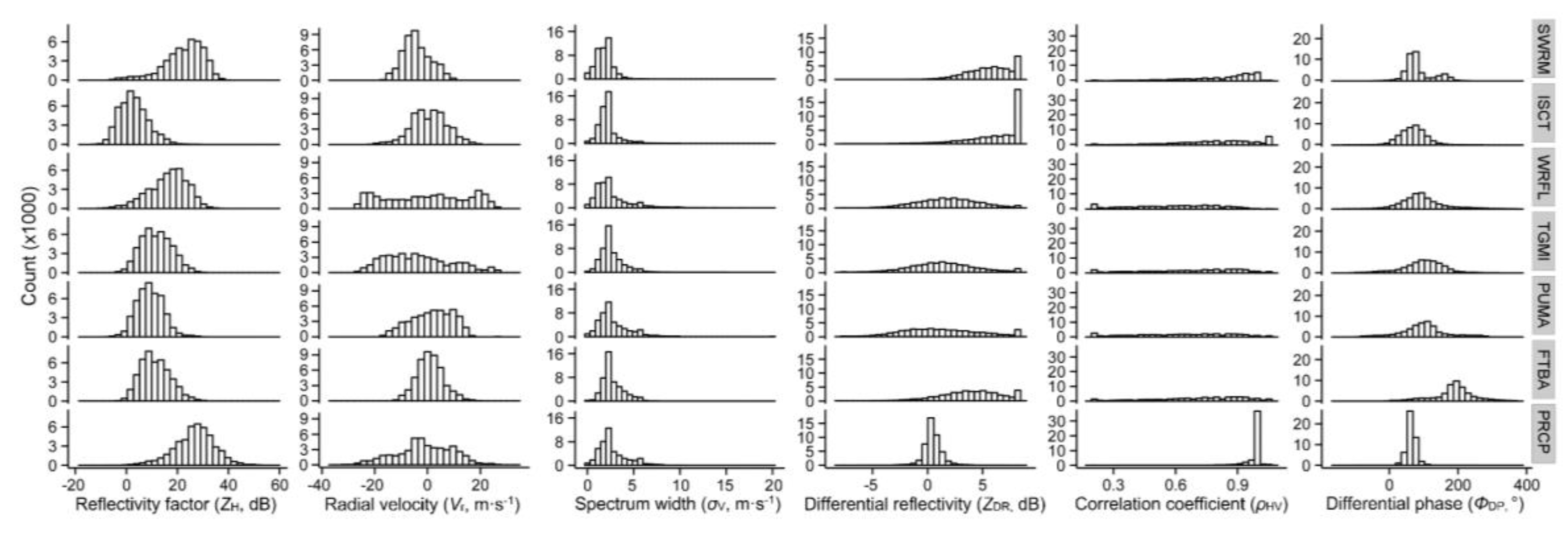
Training and classification included only resolution volumes with values available for all six radar variables. We unwrapped and normalized total differential phase values. Those data characterized by excessive velocity aliasing (i.e., more than a few scattered wrapped samples) were removed from consideration. To differing degrees, values of all radar parameters vary with aspect of the biological scatterers relative to the position of the radar within a radar sweep [18,36]. Bias in the distribution of bioscatterer aspects could lead to RF models becoming overfitted toward over-represented aspects. To ensure relatively equal representation of aspects for a given scatterer (all but grebes, a special case described below), resolution volumes for each scatterer type were subsampled according to their distribution of aspects. Histograms of the values of the six radar variables for the seven types of scatterer (Eared Grebes excluded) can be found in Figure 1.
2.3. Development of Classification Models
We used a random forest (RF) ML algorithm [61,62] to develop a variety of radar scatterer classification models. We used the R-package randomForest v4.6-10 running under R v3.0.2 [63], and resulting models were based on terminal node sizes of 1 and 500 trees. RF as applied here is a supervised classification algorithm that provides information on the relative importance of features, used to predict membership among classes based on its ensemble approach to building decision trees. ML algorithms are sensitive to imbalance among their classes, so for all models we balanced sample size among classes by under-sampling instead of minority oversampling or some combination (e.g., Reference [64]). Across all models except those involving grebes, we randomly under-sampled individual classes to a reference sample size, that of the smallest class size, specifically, purple martins (Table 1). Learning curves suggested only modest increases in performance using larger sample sizes (e.g., Figure A2), at least within our datasets.
We generated numerous RF binary and multinomial models to address the objectives described above. The models varied primarily in their variable sets and degree to which they aggregated different bioscatterer types into a single class (Table 2). The most aggregated model combined all bioscatter classes listed above (again with the exception of grebes) into a “biological” class for discrimination from rain. Another set of models moderately aggregated bioscatter types into “vertebrates”, which combined waterfowl, trans-gulf migrant birds, martins, and free-tailed bats, and “arthropods”, which combined swarming and diurnal insects. Vertebrates and arthropods were discriminated from each other and precipitation in multinomial and binary models that included only a focal type (e.g., vertebrates) and “other”. The largest collection of models focused on the discrimination of individual non-aggregated types (e.g., trans-gulf migrants, free-tailed bats), again as multinomial models that included all types, or binary models that discriminated between a focal type and “other”. Non-metric multidimensional scaling (MDS) based on model results was used to visualize similarities between non-aggregated types. For all aggregated classes in the above models (biological, vertebrates, arthropods, and “other”) each of the underlying scatterer types that comprised these classes were randomly subsampled so as to be equally represented in the aggregated class, which itself did not exceed the reference sample size.
Eared grebes represented a special case that allowed an examination of the influence of natural history on model performance. Samples came from a single radar (KMTX near Great Salt Lake, Utah) and nearly all the departure movements were confined to a corridor nearly due south of Great Salt Lake between the Stansbury and Oquirrh Mountain ranges. Occasionally, a second and parallel movement occurred through an adjacent valley to the west between the Stansbury and Cedar Mountains. Owing to their special characteristics, grebe class samples were not included in any of the aggregate classes described above. However, two binary grebe-centric models were developed that were similar to the above models that focused on individual non-aggregated types. Class sample sizes in these models were balanced based on the sample size of the grebe class (21,815 resolution volumes), and this sample size was the basis for evenly sampling all other scatterer types in generating the “other” class. One grebe-specific model was based on the six radar variables common to most of the models described above; a second model added azimuth and range to the variable set (Table 2).
Evaluation of classification results was based on the standard output of RF models, consisting primarily of confusion matrices, classification errors, and feature importance indices (i.e., mean total decrease in node impurity for a variable) based on the bootstrapped out-of-bag resolution volumes, which comprised approximately one third of the overall training datasets. Classification errors (CE) showed the proportion of incorrect classifications. A general importance or gini index was used to show the relative importance of the variables that characterized a class and was calculated by measuring the total decrease in node impurities from splitting on the variable averaged over all trees.
Finally, we used examples of discretely occurring precipitation and biological data external to the model development process in two separate case studies to examine the effects of model aggregation, data retention, and scatterer mixing on the probability of class membership. RF is one of several machine-learning algorithms that generates these probabilities, in this case based on votes from all classification trees. We did this for models using all six radar variables and representing multiple levels of class aggregation, outlined in Table 2; specifically, and depending on the case, high (biological–precipitation), medium (vertebrates–arthropods–precipitation), and low (SWRM–ISCT–WRFL–TGMI–PUMA–FTBA–PRCP).
3. Results
3.1. Backscatter Values from Seven Types of Scatterer
The values of the six radar products used in developing the RF classification models reflected the phenotypes (morphology and behavior) of the scatterers that produced them. Histograms of the values of the six radar products for each type of scatterer examined in this study can be found in Figure 1, and the median, 25th, and 75th percentiles of each radar parameter for each class (excluding EAGR) can be found in Table A2.
3.1.1. Reflectivity Factor
The histograms of reflectivity factor in Figure 1 and median values of these histograms in Table A2 overlapped to varying degrees for the seven types of scatterer, but the median value for precipitation was highest, followed by those for swarming insects and waterfowl. The histograms for trans-gulf migrants, purple martins, and free-tailed bats showed broad overlap, and the three median values were within 2 dB. The lowest median value for reflectivity factor was produced by broad-front movements of insects.
3.1.2. Radial Velocity
The median values of radial velocity tended to be close to zero because the inbound velocities (negative values) and outbound velocities (positive values) were similar. Although greatly influenced by the wind and air speed of the scatterer, the maximum inbound and outbound values of radial velocity were the greatest for waterfowl and trans-gulf migrants. Precipitation also had a wide range of values because of the velocity of the airmass containing the rain. The median value of broad-front insect movements was 6 msec−1 higher than that for swarming insects.
3.1.3. Spectrum Width
The median values of spectrum width for all types of scatterer ranged from 1.5 to 2.5 ms−1, and the distribution of the values in the histograms was similar. As mentioned below, spectrum width had the lowest importance value for discrimination of scatterer type across all types.
3.1.4. Differential Reflectivity
The histograms for differential reflectivity for swarming insects and insects moving on a broad front were shifted to high dB values (median values of 5.9 dB and 7.4 dB, respectively). The high count of highest values resulted from limiting the scale of values to 7 dB when higher values existed. The ZDR patterns of values for waterfowl, trans-gulf migrants, and purple martins were similar and showed a broader distribution of values (medians of 1.9 dB, 1.3 dB, and 1.0 dB, respectively). The range of histogram values for free-tailed bats was less broad than that for the bird scatterers and the median was shifted to a higher value (4.1 dB). The slight increase in the number of highest values of ZDR in the histograms for bats and martins and to a lesser extent, trans-gulf migrants, suggested that some resolution volumes possibly contained only insects. The values of differential reflectivity for precipitation clustered around zero dB, and the range of values was not as broad as those for vertebrates or insects.
3.1.5. Correlation Coefficient
For the correlation coefficients, the histogram values for precipitation were above 0.9 (median of 1), and the histogram values for swarming insects and broad-front insect movement were generally high (medians of 0.9 and 0.8, respectively), with some insect values approaching those for precipitation. The distribution of histogram values was similar for vertebrate scatterers, and the medians ranged from 0.6 for waterfowl to 0.8 for free-tailed bats.
3.1.6. Differential Phase
Histogram values of differential phase overlapped extensively for insects and birds, although medians were lower for insects (69.8° and 66.6°) than those for birds (84.3° 99.1°, and 95.6°). Precipitation had a median value of 61.7°, which was just a little lower than the median for insects moving on a broad front. The histogram values for free-tailed bats were higher than those for other types of scatterer, and the median value was 186.5°. A cluster of high values in the histogram of differential phase for swarming insects could have been caused by some resolution volumes containing foraging birds. The patterns in the histograms of Figure 1 and the values for the median, 25th, and 75th percentiles in Table A2 illustrate the similarities and differences among the types of scatterer and provide some insight into the results that follow on aggregation of types of scatterer, classification confusion matrices, and importance values of radar products for scatterer identification.
3.2. Aggregation and Phenotype
Among binary RF models, those aggregating more biological types into a single class classified with greater accuracy than low-aggregation models. At the highest level of aggregation, “biological” and “precipitation” resolution volumes were classified with 98.7% and 97.8% accuracy, respectively (Table 3). By comparison, classification performance of binary models decreased somewhat as broad biological types, arthropods and vertebrates, were separated and independently classified against all other types (identified as “other” in tables; Table 3). The tendency toward lower classification performance with decreased levels of aggregation continued with the non-aggregated types (Table 4). An exception concerns one model trained specifically to distinguish a passerine-dominated group, trans-gulf migrants, from diurnal insects (Table 4, last model)—a discrimination of interest in many biological applications of radar. This model outperformed all other medium- and low-aggregation models.
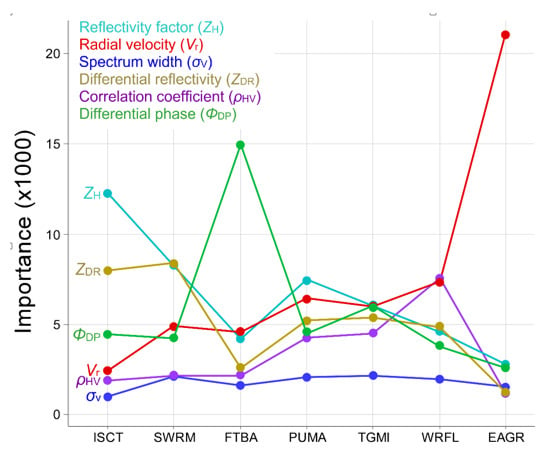
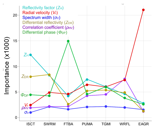
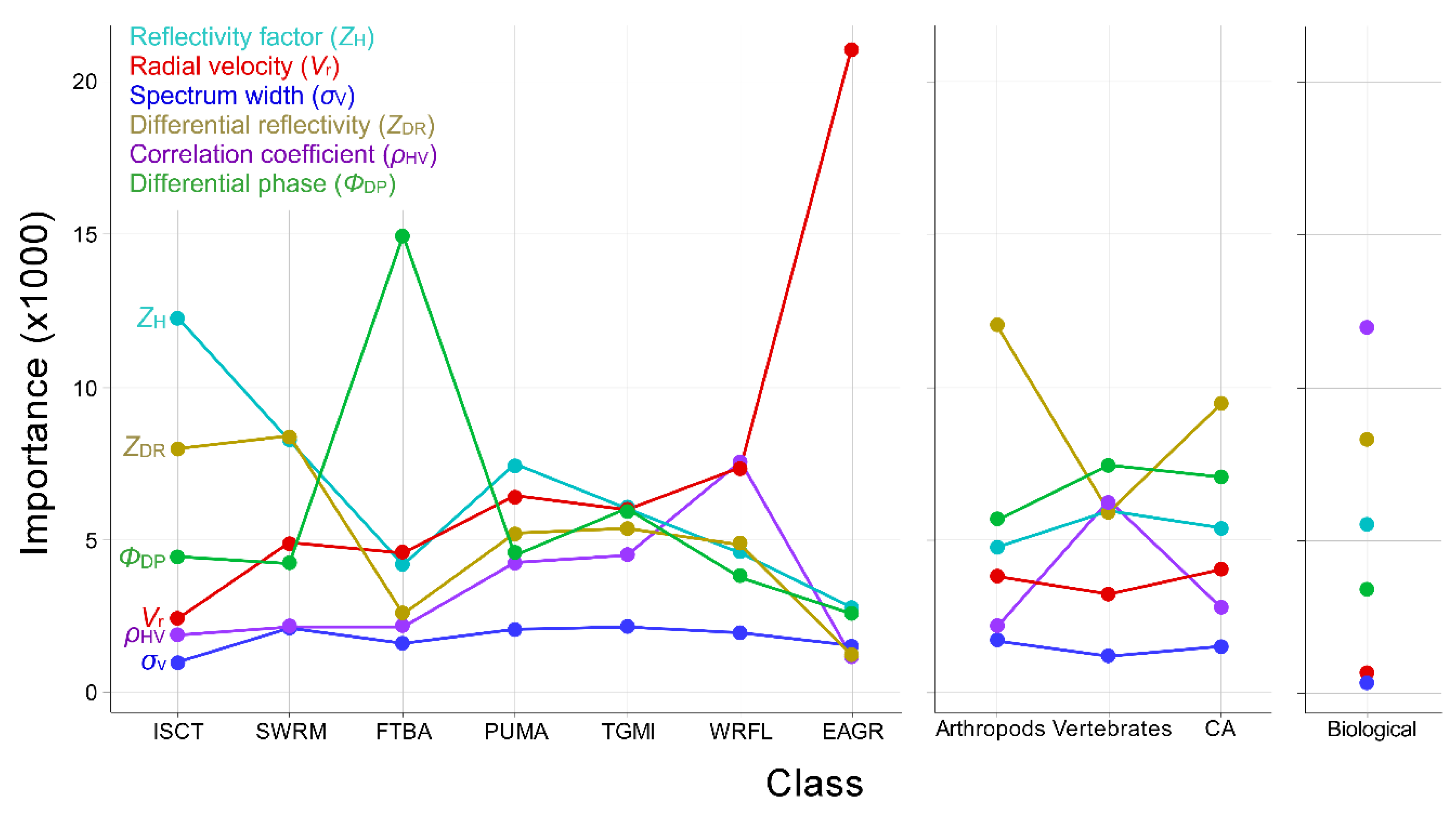
Not surprisingly, bioscatterers sharing similarities in phenotype tended to misclassify against one another more frequently than against more dissimilar types. The greatest degree of misclassification occurred among vertebrates (Table 5a), which is to say they shared broad similarities in their radar metrics where goodness-of-fit in a multidimensional scaling representation of similarity in the confusion matrix, or stress, was 8.61 × 10⁻³ (values ≤ 0.05 are considered good fits (Figure 2); importance indices bore this out. More scatterers were misclassified as martins than any other type, i.e., martins had the highest median error contribution rate (Table 5a, bottom row).The three avian classes common to these models (martins, trans-gulf migrants, and waterfowl) exhibited general similarities in the relative importance of radar variables to their classification, perhaps most notably that none of the radar variables contributed disproportionately to classification (Figure 3). Bats differed from the other vertebrates in that differential phase (ΦDP) contributed substantially to their classification. Nonetheless, bats were most frequently misclassified as martins (Table 5a). Although swarming insects were most commonly misclassified with diurnal insects, the diurnal insects in turn were most commonly misclassified as martins (although in neither case was the rate of misclassification high). Radar reflectivity (ZH) weighed most heavily in both diurnal insect and martin classification, but an examination of Figure 1 suggests that broad-front movements of insects had lower values of reflectivity than swarming insects. Discrimination of arthropods and precipitation was strongly influenced by the importance of differential reflectivity (ZDR) and correlation coefficient (ρHV), respectively.
3.3. Radar Product Combinations
The availability of polarimetric data had a large influence on model classification performance. Among medium-aggregation models, the mean classification error rate among classes using only legacy variables was 27.6% (Table 6b). Including polarimetric variables reduced the error rate to 5.6% (Table 6a; and polarimetric variables alone classified with a 12.2% error rate, Table 6c). The addition of polarimetric variables to models reduced classification error rates by 16.7% and 26.0% among vertebrates and arthropods, respectively, where differential reflectivity (ZDR) played an important role in discriminating arthropods from vertebrates Figure 1 and Figure 3). Although most radar variables proved valuable in discriminating among classes (Figure 3), spectrum width contributed least toward classification across all scatterers (Figure 1 and Figure 3) and could likely be excluded from models with little effect on classification performance. Among low-aggregation multinomial models, the mean classification error rate among classes using only legacy variables was 45.6% (Table 5b). Including polarimetric variables reduced the mean error rate to 20.5% (Table 5a; polarimetric variables alone classified with a 42.5% mean error rate, Table 5c). Among biological classes, including polarimetric variables resulted in the greatest improvement in classification accuracy of martins and waterfowl, reducing error rates by 31.6% and 28.8%, respectively. Among models trained exclusively on polarimetric variables, error rates for four of the six biological classes were higher than for models trained exclusively on legacy variables. Classification of precipitation, and to a lesser degree of waterfowl and bats, improved with polarimetric variable models. The model variable set also had a large influence on the class with the highest false positive classification rate. The only broad pattern across all low-aggregation multinomial models was general confusion among vertebrates (Table 5a–c). This confusion was particularly acute for martins in the polarimetric variable model where the false positive rate for waterfowl (32.7%) exceeded the true positive rate for martins (27.7%); this was the only instance across all models in the study where a false positive rate exceeded a true positive rate, and was likely a side-effect of model complexity and the central place waterfowl occupy in the radar polarimetric variable space (see EC for waterfowl, Table 5c).
3.4. Natural History, Data Retention, and Mixed Scatterers
The distinctiveness of eared grebe departures from Great Salt Lake helped to ensure identification of their radar backscatter, but also introduced extreme bias in their radar scattering parameters. Grebe backscatter was characterized entirely by movement away from Salt Lake City, Utah radar (KMTX), and nearly all of those movements occupied a narrow range of azimuths ( ± SD = 180.8° ± 4.7°) between 80 and 160 km from the radar. Given the well-defined movement corridor and speed of flight ( ± SD = 19.1 ± 6.2 ms−1) directly away from the radar, grebes classified against all other scatterers with high accuracy (97.5%), largely based on the overwhelming importance of radial velocity (Vr; Table 7a, Figure 3). Including range and azimuth along with the six radar variables in a binary model classifying grebes against other scatterers increased classification accuracy to 99.8% (Table 7b). Range and azimuth were second and third most important to classification behind velocity.
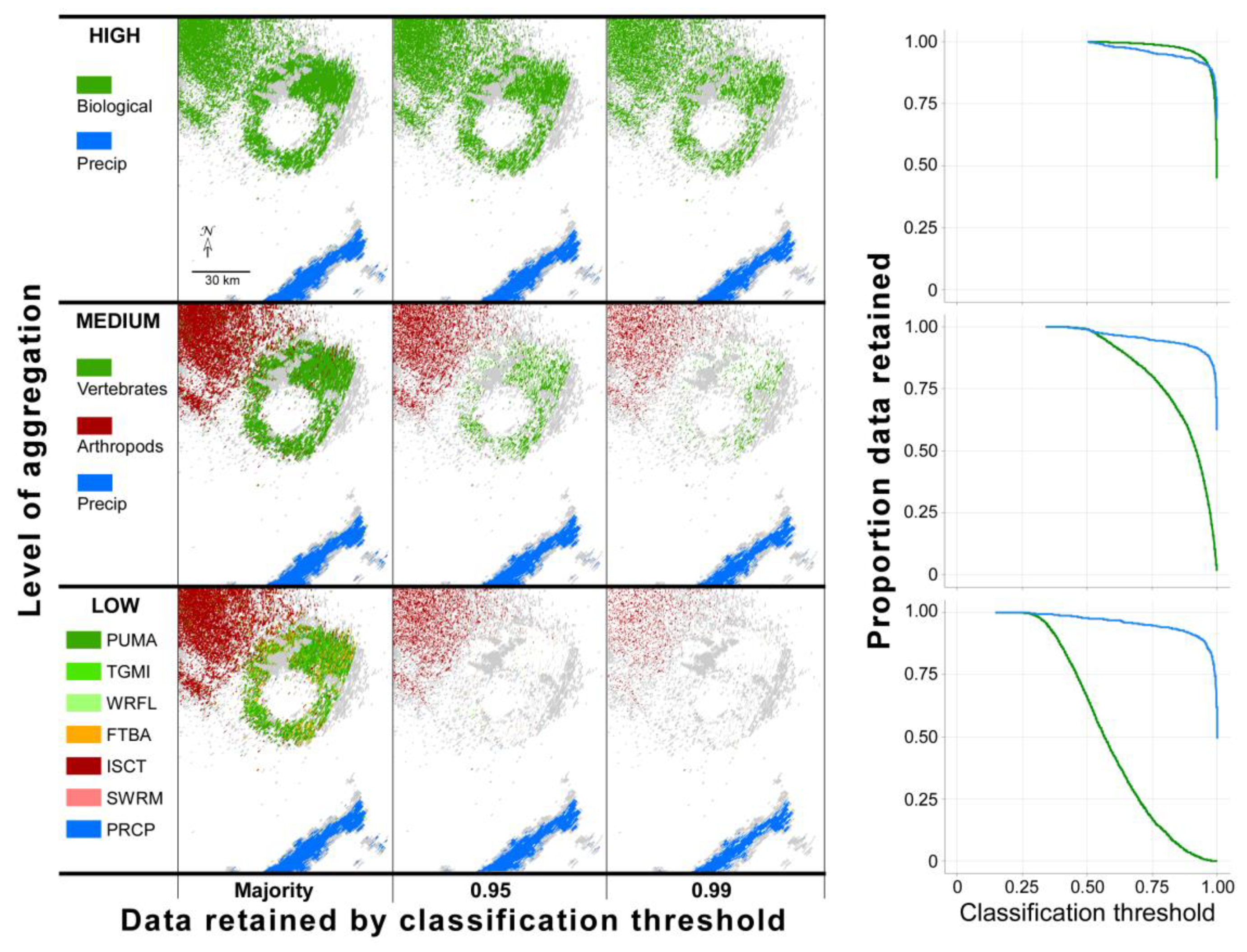
The high true positive rate for grebe classification suggested the possibility of setting high classification probability thresholds while still retaining most of the resolution volumes of interest for further analysis. The results of our exploration of data retention with different probability thresholds in a case study using models tested against data excluded from model development are illustrated in Figure 4. This figure shows a radar sweep containing mixed precipitation and biological data classified using three models that varied in aggregation. For each of these, data retained at each of three probability thresholds are shown and highlight the trade-off between the relatively high model performance associated with aggregating classes and bioscatter detail associated with multi-class models. With high aggregation, large proportions of data were retained even under high probability thresholds. By comparison, low-aggregation models that forced discrimination among more classes retained little biological data with high probability classification. Precipitation and arthropod/diurnal insect classification proved more resistant than vertebrate classification to the effects of lower levels of aggregation, again owing to the disproportionately high importance of correlation coefficient and differential reflectivity/reflectivity, respectively (Figure 3).
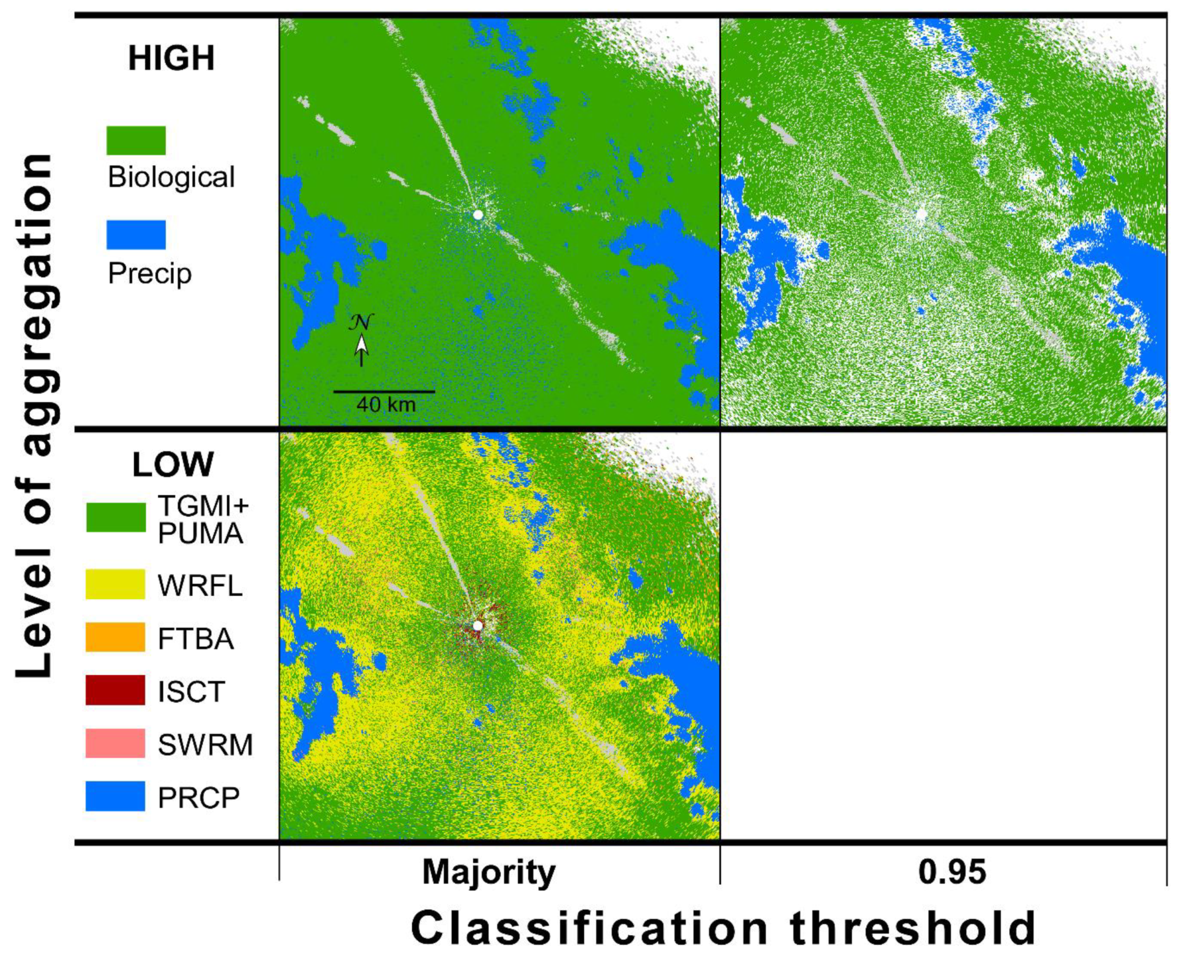
Scatterer types in the above case were largely spatially distinct from one another. However, in a second case study where precipitation and biological scatter occurred in close proximity, resolution volumes containing mixed scatterers influenced their classification. The high-aggregation model applied to these data showed exceptionally low retention of high probability resolution volumes where biological and meteorological scatterers met, which appear as white space in regions bordering precipitation in Figure 5. A low-aggregation model applied to this same sweep showed that many of these presumably mixed resolution volumes were misclassified as waterfowl.
4. Discussion
4.1. Previous Studies
Rennie et al. [12] pointed out that the ultimate requirement of a classifier is to discriminate echoes by usefulness, rather than to accurately identify all echo types, since accurate identification of echo types using a single-polarization classifier is difficult. Prior to dual-polarimetry, some studies used information on the air speed of the scatterer for identification (e.g., birds have higher air speeds than insects) [9,23,24], and other studies relied on knowledge of natural history (e.g., day-active in summer or night-active during migration seasons) [19]. In some cases, two different types of radar were used to separate returns from birds and from insects [20,65].
Once dual-polarization was available, some investigators used one or more of the approaches mentioned above to identify the type of scatterer and to characterize the values of the polarimetric variables produced by that type of scatterer [36]. In most of the studies that have reported values of polarimetric variables from biological scatterers, the authors made assumptions about the identity of the type of scatterer before the analysis of the polarimetric data, but in a few cases the investigators knew the identity of the scatterer [66] or they knew about the departures of purple martins and other swallows from nighttime roosts [18,51,67,68] and the exodus of free-tailed bats from their daytime roosts [18,49,51,69]. In our study, we recorded legacy and polarimetric data from known biological scatterers and rain and generated histograms of values (Figure 1) for each type of scatterer. The values were similar to those reported previously for purple martins, insects, and rain [18] and the polarimetric values reported in additional studies devoted to the classification of different types of scatterer (Table A3, Table A4 and Table A5).
4.2. Aggregation, Variable Importance, and Phenotype
We included models that varied in the degree to which they aggregated biological scatterers into a single class in a manner consistent with the kinds of analyses currently conducted and with a view toward future applications. Not surprisingly, model classification accuracy tended to increase with the degree of aggregation and variable importance changed with the level of aggregation and scatterer type. At the highest level of aggregation, binary models that discriminated between biological and meteorological scatterers were among our best performing, primarily owing to differences in correlation coefficient, with differential reflectivity, reflectivity, and differential phase playing a lesser but likely meaningful role. Our measures of correlation coefficient for different scatterers were broadly consistent with those of other studies (Table A2), and there is general agreement in the literature that correlation coefficient is especially useful for discriminating between biological and meteorological scatterers. Among medium-aggregation models, differential reflectivity was most important for separating arthropods from vertebrates (see previously reported values of differential reflectivity in Table A3), and differential phase was most important for separating vertebrates from arthropods (see previously reported values of differential phase in Table A5). These findings are generally supportive of those reported by Zrnić and Ryzhkov [36], and several subsequent studies by other investigators have used these findings as a basis for identifying polarimetric returns from birds and insects (e.g., References [42,70]). Generally, classification accuracy among the least aggregated binary models was slightly lower and more variable, primarily owing to the inclusion of more types similar to the focal type in the “other” class against which focal types were discriminated. Variable importance depended highly on the focal type. The high performance of some low-aggregation models tended to be associated, with specific radar metrics playing a disproportionately large role in their classification. That discrimination between meteorological and biological scatterers, and more specifically between vertebrate and arthropod bioscatter, is nearly a prerequisite for functional radar aeroecology speaks to the importance of these two variables in future biological applications of polarimetric radar.
Both physical and behavioral aspects of flying animals are relevant to their distinctiveness from one another as radar scatterers. This paper focused on differences in radar parameter space at the level of the resolution volume, so variation in behavior among scatterers was not considered directly in most cases but nonetheless may have manifested indirectly in the discrimination, e.g., with respect to radial velocity. Differences in the aspect ratios of scatterers strongly influence their polarimetry values [18,44,45,51,71] and allow for their partial discrimination. Aspects of the animal with respect to the radar may be the single greatest source of variation in backscatter values. Values of the polarimetric variables and reflectivity are sensitive to the cross-sectional area and shape of the scatterer [18], specifically the aspect ratio of the lateral to the rostral/caudal area as presented to the radar. Meteorological and biological scatterers occupy different places along the continuum of aspect ratios from oblate to prolate to extreme prolate spheroids for precipitation, vertebrate, and (with exceptions) arthropod scatterers, respectively. Depending on the metric, the bilateral symmetry or asymmetry through 360° of weather radar data often characteristic of flying animals likely results from a combination of factors including degree of shared orientation, variation in pitch during flight (which introduces tri-axial aspect dependence), and the so-called STAR approach to polarimetry characteristic of the WSR-88D [44]. Differences in aspect effects were most clearly evident in the values of backscatter of differential reflectivity among vertebrates, arthropods, and precipitation. Among vertebrate scatterers, differences in aspect ratio become more subtle, likely forcing refined methods of discrimination to rely more heavily on behavior and other aspects of natural history. Even then, a sufficient radar and natural history parameter space may not always exist between groups of animals to allow for their reliable discrimination.
In our low-aggregation multinomial model, martins were responsible for more classification error than any other class, presumably because this species sits at a morphological and behavioral intersection with other vertebrates which comprise four of the seven classes considered. The trans-gulf migrant class contains a mixture of different types of birds (e.g., passerines, shorebirds, herons and egrets, and waterfowl) flying individually or in flocks [55], and the values of the radar variables for trans-gulf migrants and other bird class types (martins, waterfowl) showed considerable overlap (Figure 1). Purple martin, trans-gulf migrant, and free-tailed bat bodies overlap in size and shape, and martins and free-tailed bats share similarities in behavior as resolution volumes used in classification for both species were drawn from roost departures. In the context of this study, removing martins from models should have the greatest impact in reducing classification error, even in many binary classifications where the “other” category includes martin samples.
Free-tailed bats emerge from daytime roosts in a meandering stream [49,69] and, consequently, the echo pattern on radar is not always in the shape of an annulus, as it tends to be with martins. We found that the differential phase was most important in distinguishing free-tailed bats from other types of scatterers. Phase values associated with bats exceeded 100°, and the values did not appear to vary consistently as a function of flight direction, as was the case for the departure of martins from overnight roosts. For some colonies, bats flying away from the radar had lower phase values than those flying in other directions, but not all roost departures exhibited this pattern. It is unclear why bats exhibited higher differential phase values than other vertebrate bioscatterers. Systematic bias associated with individual radars seems unlikely, since the bat data used in model training and testing originated from five different radars. Bats may differ phenotypically from other aerial vertebrates dielectrically (e.g., internal anatomy, a membranous patagia) and behaviorally (e.g., possibly greater diversity of orientations within a resolution volume) in ways that meaningfully influence phase, but how that biology might interact with differentially polarized energy to influence phase is unknown and an area that requires further study [72].
4.3. Natural History
Use of natural history (e.g., geographic range, altitude, time of year, time of day, flight behavior, and any number of correlated predictors) to constrain models should considerably increase classification performance under most circumstances. Contemporary natural history data and information are now available through a variety of sources including eBird [73], running updates on species accounts [74,75], and wildlife management agencies [76]. A thorough assessment of the influence of incorporating natural history into classification models was beyond the scope of this paper, although the known migratory departures of eared grebes southward out of Great Salt Lake, Utah offered a simple case study [60]. Grebe backscatter violated a number of criteria required for their inclusion in other models (e.g., single radar, narrow range of azimuths), but such bias can be harnessed to build models designed to detect specific events or phenomena with high accuracy, and as a result their radar characterization could be narrowly specified, which improved classification performance. A grebe binomial model trained based on all radar variables plus azimuth and range to capture some spatial natural history (this was the closest any model came to capturing spatial patterns) showed excellent classification performance locally but at the cost of generalization, for example by severely penalizing the detection of grebes in other regions of the sweep. As with multinomial versus binary models, there was likely a trade-off between model performance and generality.
Where the natural history of flying animals is well established, numerous opportunities exist to develop narrowly trained classification models as event detectors; for example, waterfowl departing known lakes and reservoirs [47] or martins, swallows, and bats departing traditional roosts [49,67,77]. Exceptionally high performing models may be able to screen for uncommon or rare events, e.g., occurrence of a taxon in an unusual geographic location or at an unlikely time. Such narrowly specified yet highly reliable models allow automated enumeration of animal abundance and density, especially since considerably fewer assumptions or less guesswork are involved in estimating radar cross-sections. Such a capability would in turn enable near real-time biological monitoring of events that have high economic or human safety considerations (e.g., informing smart curtailment with wind energy, flight safety).
4.4. Data Retention
In our case study, two trade-offs emerged that influenced data retention. First, as the threshold probability of a given classification increased, fewer data met that threshold and the proportion of data retained decreased. Second, the models that discriminated among fewer classes and/or aggregated similar types into more inclusive classes retained more data at higher probability thresholds (models like these are also more likely to be used in real-world applications). Radar applications must balance this three-way compromise between model complexity, acceptable probability of classification, and proportion of data retained. There seems to be a tendency among weather radar studies to favor data retention over other considerations, in part due to the inherently appealing comprehensiveness of radar datasets. High data retention is justified where the signal of interest overwhelms classification error rates and may be necessary for certain applications, e.g., for example, those that rely on absolute abundance measures. However, many applications of such models can acknowledge the inevitable imperfections of machine learning’s ability to classify scatterers by accepting lower data retention thresholds in favor of greater certainty about the identity of the scatterer and still retain sufficient data for further analyses.
Consider from our first case study (Figure 4) the medium-aggregation model applied to novel data wherein >35% of data classified as vertebrate were retained at a ≥95% threshold probability of classification. The vertebrates were martins departing a roost and, at this probability of classification, samples from all directions of departure were retained, enabling quantification of relative abundance (e.g., across sweeps; between days, years), speed and direction, orientation, estimation of roost location, and so on, but with the benefit of reduced contamination from non-focal scatterers, in this case, presumed insects. (Although the insect classification in this example could not be independently confirmed, values for the resolution volumes were consistent with those of insects.)
4.5. Methodological Considerations
Recognizing that the goal of this paper was to examine differences among bioscatterers in their radar parameter space, the methods adopted here represent a rudimentary approach to bioscatter classification that in most cases does not rely on classification of scatterers beyond the out-of-bag samples. More fully developed methods of bioscatter classification with the goal of addressing specific biological questions will build more comprehensive training datasets through use of natural history and direct corroboration of scatterers and apply state-of-the-art approaches to machine learning (e.g., References [14,15,16]).
4.5.1. Training Data and Validation
Our efforts represent a best attempt based on the literature, knowledge of natural history, and secondary sources to identify training data with minimal clutter from non-focal scatterers. Ultimately, the quality of classification models stands on the quality of their training data, and to that end, our approach can be improved. The highest standard for such data would be independent verification through concurrently gathered remotely sensed data using complementary methods (e.g., portable radar, thermal imaging, and aerial insect netting) or some other form of confirmation that can reliably distinguish scatterer types. There is a dearth of such data, especially contemporaneous with the advent of polarimetry in weather radar.
The benefits of strong training data increase when the discrimination problem is subtle or poorly understood, or where the consequences of being wrong are high. Applications associated with flight safety or wind turbine curtailment are unlikely to tolerate high false positive/false negative rates. Flight safety in relation to flying animals is generally a large-bird problem. The results in this paper showed that waterfowl overlap considerably with other vertebrates in their radar parameter space, suggesting improved discrimination will rely more heavily on better algorithms likely informed by natural history and more nuanced training data. Weather radar-informed wind turbine curtailment to reduce impacts to flying animals carries an economic cost associated with higher turbine cut-in speeds [78]. Radar-based methods that govern such operations must reliably index the presence of the vertebrate of interest, which may in part turn on the quality of training data when resolution volumes routinely contain mixed vertebrate–arthropod scatterers (see below for further consideration of mixed scatterers).
4.5.2. Errors in Assignment and Classification
From the outset, it was unlikely that such a narrow parametric specification for bioscatterers would suffice for high probability discrimination among similar biological types. Still, such an approach offers the benefit of divorcing the resolution volume from the context of the broader movement patterns which are often not maintained as a movement develops. This is a key challenge facing some spatial-pattern-based discrimination algorithms. Animal movement—even when captured within a single resolution volume—is likely most organized during its early stages. For example, departures of roosting species show structure that dissolves as animals arrive in their feeding spaces. For this reason, bias in supervised classification, including that presented here, may emerge if training datasets are developed from bioscatterers identified by their echo patterns during distinct phases of movement that are most recognizable by experts.
Another source of classification error arises from radar-system-specific variability. Operational settings such as radar wavelengths and values of the initial system differential phase often differ slightly from location to location [18], and these differences impact the values of radar moments used in training. Although properties such as wavelength are fixed for a given radar, the radar’s operating mode is not and can be adjusted depending on weather conditions. Modes of operation that favor rapid updates in support of severe weather monitoring adjust data collection (with respect to, for example, antenna rotation and pulse length) in ways that reduce radar sensitivity. Importance measures of radar metrics show that classification of non-swarming insects depends strongly on radar reflectivity particularly because its values are skewed toward weak echoes for this class. Loss of weak echoes therefore has a disproportionately negative impact on arthropod discrimination and associated quantification. Vertebrate echoes are also impacted but to a lesser degree (R. Diehl, pers. obs.).
In addition, biological scatterers often present as non-beam filling, a key assumption in many quantitative radar biological and meteorological applications. Consider flocking waterbirds. Location within the beam is unknown, as are the positions of the animals relative to each other and relative to the radar’s view. Through successive sweeps, the same flock of waterbirds flying in row or v-formation presents to the radar in a range of orientations that may cause birds to be variously obscured or electromagnetically interacting with each other relative to incoming pulses, resulting in scattering properties that are extremely difficult to predict. Moreover, it is not unreasonable for a single resolution volume to contain varying combinations of Rayleigh, Mie, and optical scatterers (e.g., insects, songbirds, geese—see below). Other confounding (and interacting) factors that influence radar measures include possible variation in pitch angle between types of flying animals, variable Mie scattering properties associated with horizontal versus vertical polarization, uncertainty about dielectric constants associated with diverse tissues, and, not least, aspect effects of the scatterer (see below). Collectively, these and still other factors contribute to a din of uncertainty that will continue to complicate the discrimination of scatterers.
4.5.3. Mixed Scatterers
In developing our training datasets, we attempted to avoid resolution volumes containing mixed scatterer types, but such mixing is common and some degree of cross-contamination from non-focal scatterers in our data was inevitable. The radar parameter values of mixed scatterer volumes presumably integrate qualities of the different types and, depending on the types and degree of mixing, should classify with low probability, allowing easy rejection of these data. This is likely why data retention was low at a ≥95% probability of classification in the boundary areas between precipitation and bird movement in our second case study (Figure 4). Many of these samples reverted to classification as waterfowl in our low-aggregation majority classification (we assume erroneously, given time of year and biased distribution, i.e., location with respect to precipitation). This may have been the result of waterfowl occupying a radar parameter space between migrating songbirds and precipitation, as exemplified in our MDS. The possibility of such uncertainty in interpretation complicates the use of multinomial classification models. In this paper, low-aggregation multinomial models served a diagnostic role in understanding errors in classification among types of scatterers. Moreover, the classes in these models often do not co-occur for reasons of natural history, so such models are unlikely to find much application where classification performance matters.
One of the most common occurrences of scatterer types mixing within resolution volumes concerns vertebrates, usually birds, and arthropods. We attempted to minimize the presence of arthropods in small-bird training data by selecting samples from migration events over the Gulf of Mexico on the assumption that arthropod movement arriving from over the Gulf is limited. Like any form of noise, the relevance of arthropods as clutter should be balanced against the magnitude of the signal one is trying to detect, assuming this can be known. Many vertebrates are Mie and optical scatterers at S-band (the wavelength of weather radars in the US), and therefore often account for most radar reflectivity when co-occurring with arthropods, which are much weaker Rayleigh scatterers [18]. Arthropods may introduce little meaningful radar clutter in most vertebrate studies, although this will vary with timing and location, and the magnitude of arthropod clutter in mixed resolution volumes is not well known. When the impact of a non-focal taxon on classification of resolution volumes is known to be minor or inconsequential to the question at hand, classification performance may be improved by purposefully training on resolution volumes containing mixed bioscatterers. Our trans-gulf migrant class is an example of this. Small birds likely dominated the class, but it included a wide range of shorebirds and other larger waterbirds.
Despite their presence as weaker echoes in radar data, arthropods often far outnumber vertebrates. Understanding more about arthropod contributions to these mixed resolution volumes may be critical to studies that focus on arthropods and their role in aeroecology. Such discrimination would require careful parsing of mixed resolution volumes for the arthropod contribution, which would rely on training data associated with the known proportional contribution of vertebrates and arthropods to resolution volumes. Efforts to identify the types of scatterers and their proportions in resolution volumes may require different types of radar and remote sensing [20,23,79,80,81,82]. Bachmann and Zrnic [40] used polarimetric spectral densities to estimate the mixed content of resolution volumes. Their procedure requires access to low-level radar data that is not typically archived for use by researchers, but select access to such data may serve as a method for building training data sets or otherwise validating classification models focused on finer discrimination between songbirds and arthropods in mixed resolution volumes. The Bachmann and Zrnic [40] method might also be applied to other common mixtures of biological scatterers.
4.5.4. Radar Variable Combinations
Differences in performance of classification models built from full radar variable sets, legacy variables, and polarimetry variables are relevant to the kinds of questions that may be asked of these data. Decadal datasets are required to assess climate, land use, or other medium- or long-term changes that may impact aerofauna. The addition of polarimetry to the WSR-88D was completed in 2013 and, as of this writing, only a few studies have used polarimetric data to develop algorithms that can filter rain from legacy non-polarimetric data for use in studies of long-term changes in bird migration [15,16] or to find features such as martin and swallow roosts [68]. Inclusion of polarimetry variables allows the shapes of scatterers to play a much greater role in their discrimination, thereby considerably reducing classification error rates among all scatterer types. Lin et al. [14] overcame the constraints of polarimetry’s brief history by relying on the relationship between high correlation coefficients and precipitation to develop large training datasets that helped to build general but reliable bioscatter classification models based only on historic three-moment data.
The radar variable set used during our model construction strongly influenced classification performance. The strong influence of correlation coefficient on precipitation classification increased the influence of polarimetric variables on classification performance overall, an effect that was more pronounced in more highly aggregated models where the precipitation class comprised a greater proportion of classifications. For medium-aggregation models (vertebrates, insects, and rain), we found the classification error rate among classes using only legacy variables was 27.6%, and when polarimetric variables were included, the error rate declined to a mean of 5.6%. Radhakrishna et al. [83] also demonstrated improved classification performance of fuzzy logic algorithms that discriminated precipitation from migrating birds by including dual-polarimetric variables. They examined two independent events, one consisting of precipitation without birds and the other with only birds. The misclassifications were 10.12% and 9.6%, respectively, for the non-polarimetric algorithm, and 1.99% and 0.92% for the polarimetric algorithm. Accurate classification of arthropods and precipitation relied more on polarimetry variables than that of vertebrates, but all groups benefitted. This complicates discriminating arthropods from vertebrates in biological datasets that predate the deployment of polarimetry.
5. Conclusions
In this study, we examined how well combinations of values of non-polarimetric and polarimetric return distinguished among known biological and rain scatterers. Our results identified how different forms of bioscatter varied from one another in their six-variable radar parameter space. We found the greatest distinction between meteorological and biological scatterers, and within biological scatterers, between arthropods and vertebrates. We suggest that data on validated scatterer identity, density, and body orientation with respect to the radar; spatial patterns of echo return; and natural history will advance approaches to bioscatter classification. The resulting future algorithms will enable the application of data from weather surveillance radar to assist in improving flight safety [67,84], monitoring the movements of agricultural pest and disease vectors [85], making informed conservation decisions [86,87], and providing the public with information that will enhance wildlife viewing opportunities [88].
It is extremely challenging to know the scattering properties of flying animals. They are comprised externally of chiton, feathers, fur, or flesh and contain anatomically complex hard and soft tissues arranged in an enormous variety of body shapes and sizes that are not radially symmetric. Animal shape interacts with body orientation and pitch angle to present a highly variable and dynamic surface to incoming radar pulses. As discussed above, there exists a long list of unaccounted factors that influence radar measurement. Taken together, these sources of variation would result in radar parameterizations that have a large number of possible overlapping valuations that likely place limits on certain forms of quantification.
Even as we overcome challenges to use current weather radar platforms, successors to these systems are being planned [89,90]. What are the implications for future weather radar platforms—probably phased-array radar—for studies of flying animals? To what extent is the research we are conducting now on biological scatterers weather-radar-platform-specific? Will proposed weather-surveillance radar systems advance or retard our ability to study flying animals? Are biological considerations part of the discussion in the design of future weather radar platforms, and are current biological applications of weather radar helping our own relevancy in that discussion? Although unlikely, should existing weather radar systems persist in support of biological data collection and continuity despite the adoption of new technologies for meteorological purposes?
Supplementary Materials
The base dataset used in the analysis can be found in the Zenodo repository (https://zenodo.org/record/3635974#.XkOW_XERXIU).
Author Contributions
Conceptualization and sample selection, S.G.; Methodology and analysis, R.D.; Writing—original draft, S.G.; Writing—review & editing, R.D. All authors have read and agreed to the published version of the manuscript.
Funding
This research project was initiated while S.G. held a position of Visiting Scientist funded by a Cooperative Agreement 12-G-015 and 17-G-014 between the Center of Excellence in Airport Technology (CEAT), Department of Civil and Environmental Engineering, University of Illinois at Urbana-Champaign and the Federal Aviation Administration of the U.S. Department of Transportation.
Acknowledgments
S.G. wishes to acknowledge beneficial discussions about polarimetric weather radar with CEAT members: Edwin Herricks, Dave Mayer, Wendell Bunch, Ann-Marie Shapiro, Peter Lazar, Elizabeth Woodworth, and Sid Majumdar. Jill Deppe and two anonymous reviewers provided helpful comments on this manuscript.
Conflicts of Interest
The authors declare no conflict of interest
Appendix A. Supporting Tables

Table A1.
Internet websites documenting WSR-88D detection of known biological scatterers that informed training/test data selection 1.
Table A1.
Internet websites documenting WSR-88D detection of known biological scatterers that informed training/test data selection 1.
1. All web sites were functional as of 24 November 2019.
Table A2.
Median, 25th and 75th percentiles of each radar parameter for each class (excluding EAGR). Values correspond to distributions in Figure 1.
Table A2.
Median, 25th and 75th percentiles of each radar parameter for each class (excluding EAGR). Values correspond to distributions in Figure 1.
| Type | Reflectivity | Radial Velocity | Spectrum Width | Differential Reflectivity | Correlation Coefficient | Differential Phase | ||||||||||||
|---|---|---|---|---|---|---|---|---|---|---|---|---|---|---|---|---|---|---|
| Med | 25% | 75% | Med | 25% | 75% | Med | 25% | 75% | Med | 25% | 75% | Med | 25% | 75% | Med | 25% | 75% | |
| SWRM | 23.5 | 18.0 | 28.0 | −5.0 | −7.5 | −0.5 | 1.5 | 1.0 | 2.5 | 5.9 | 4.4 | 7.4 | 0.9 | 0.7 | 1.0 | 69.8 | 58.2 | 91.7 |
| ISCT | 2.0 | −1.5 | 6.0 | 1.0 | −4.0 | 5.5 | 2.0 | 1.5 | 2.5 | 7.4 | 5.1 | 7.9 | 0.8 | 0.7 | 1.0 | 66.6 | 42.0 | 88.9 |
| WRFL | 17.0 | 11.0 | 21.5 | 0.0 | −14.5 | 13.0 | 2.0 | 1.0 | 3.5 | 1.9 | −0.1 | 3.8 | 0.6 | 0.4 | 0.8 | 84.3 | 55.0 | 117.4 |
| TGMI | 11.0 | 7.0 | 15.5 | −5.0 | −13.5 | 5.0 | 2.5 | 1.5 | 3.0 | 1.3 | −0.5 | 3.3 | 0.7 | 0.5 | 0.9 | 99.1 | 63.1 | 133.2 |
| PUMA | 9.0 | 5.0 | 12.0 | 2.5 | −4.0 | 8.0 | 2.5 | 1.5 | 3.5 | 1.0 | −1.3 | 3.6 | 0.7 | 0.5 | 0.8 | 95.6 | 61.3 | 123.7 |
| FTBA | 10.5 | 6.5 | 14.5 | 1.0 | −2.5 | 4.0 | 2.5 | 2.0 | 3.5 | 4.1 | 2.2 | 5.9 | 0.8 | 0.6 | 0.9 | 186.5 | 160.7 | 210.8 |
| PRCP | 27.0 | 22.0 | 31.5 | −1.5 | −7.5 | 7.0 | 2.5 | 1.5 | 3.5 | 0.4 | 0.0 | 0.8 | 1.0 | 1.0 | 1.0 | 61.7 | 53.6 | 67.7 |
Table A3.
Examples of correlation coefficient values for different types of scatterers.
| Correlation Coefficient | ||
|---|---|---|
| Type | Value | Reference |
| Pure rain and dry hail | >0.98 | [27] |
| Wet hail | <0.95 | [27] |
| Very large hail | <0.85 | [27] |
| Weather | >0.8 | [91] |
| Light to moderate rain | >0.99 | [91] |
| Heavy Rain | >0.97 | [91] |
| Non-meteorological | <0.85 | [30] |
| <0.80 | [27] | |
| <0.65 | [34] | |
| Biological | 0.3 to 0.5 | [36] |
| 0.5 to 0.8 | [51] | |
| 0.3 to 0.7 | [92] | |
| <0.7 | [91] | |
| Insects | 0.8 to 1 | [40] |
| 0.3 to 1.1 | [18] | |
| <0.97 | [42] | |
| 0.4 to 0.9 | [44] | |
| 0.3 to 0.8 | [91] | |
| Birds | <0.7 | [42] |
| Birds > insects | [70] | |
| Nocturnal migrating birds | 0.5 to 0.7 tail-on | [51] |
| 0.7 to 0.85 head-on | [51] | |
| Purple Martins | 0.5 to 0.8 | [51] |
| 0.3 to 1 | [18] | |
| Tree Swallows | 0.2 | [67] |
| Free-tailed Bats | 0.5 to 0.7 | [51] |
Table A4.
Examples of differential reflectivity values for different types of scatterers.
| Differential Reflectivity | ||
|---|---|---|
| Type | Value (dB) | Reference |
| Rain | 0 to 2 | [93] |
| −2 to 2 | [18] | |
| <3 | [94] | |
| Hail | Near 0 | [94] |
| Non-meteorological | >4.5 | [34] |
| Biological | >2 | [51] |
| >3 | [91] | |
| >7 | [95] | |
| Insects | 0.5 to 5 | [65] |
| 5 to 8, mean 7 | [96] | |
| 2 to 10 | [36] | |
| <10 | [97] | |
| 9 aligned | [39] | |
| 0 tail-on, head-on | [39] | |
| 0 to 3.5 | [38] | |
| 3 to 8 | [91] | |
| 4 to 6 | [92] | |
| 5 to 10 | [95] | |
| 3 to 10 | [97] | |
| about 8 | [94] | |
| 4 to 8 | [42] | |
| −4 to 8 | [18] | |
| 4 to 9 | [92] | |
| ≥8 | [68] | |
| 8 to 9 | [66] | |
| Birds | −1 to 3 | [69] |
| <4 | [98] | |
| 2.2 | [37] | |
| <2.5 | [40] | |
| −4 to 4 | [42] | |
| Nocturnal Migrating Birds | 2.5 | [99] |
| 2 to 6+ | [51] | |
| Purple Martins | 3 to 6+ | [51] |
| Tree Swallows | −8 to 4 | [67] |
| Free-tailed Bats | 1.5 to 3 | [51] |
Table A5.
Examples of backscatter differential phase values for different types of scatterers.
| Backscatter Differential Phase | ||
|---|---|---|
| Type | Value (degrees) | Reference |
| Rain | 0° with 60° offset | [93] |
| Biological | 50 to 100+ | [92] |
| Insects | <40 | [69] |
| Mean 40 | [30] | |
| <20 to 30 | [98] | |
| 5–40 | [36] | |
| <30 | [37] | |
| 50 to 80 | [40] | |
| 0 to 60 | [42] | |
| 10 to 40 | [100] | |
| Birds | >100 | [69] |
| 70 to 100 | [100] | |
| 100 | [98] | |
| 0 to 100 | [36] | |
| >70 | [37] | |
| 0 to 150, most > 60 | [42] | |
| ≥100 | [68] | |
Appendix B. Supporting Figures
Figure A1.
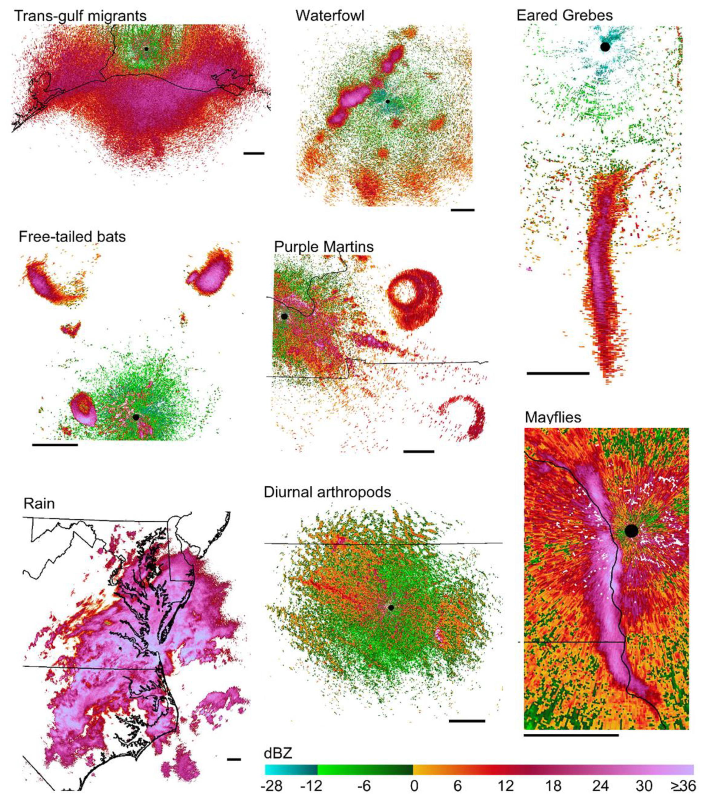
Examples of different scatterer types used in this paper shown in radar reflectivity factor. The radar call signs, dates, and times associated with each scatterer type are: Trans-gulf migrants, KLCH, 6 May 2014, 1707 CST; Waterfowl, KILX, 9 Nov 2016, 1756 CST; Eared Grebes, KMTX, 26 Nov 2014, 1931 MST; Free-tailed bats, KEWX, 3 Jul 2016, 1944 CST; Purple Martins, KPAH, 15 Aug 2014, 0507 CST; Rain, KAKQ, 8 Sep 2014, 1505 EST; Diurnal arthropods, KABR, 22 Jun 2014, 1755 CST; and Mayflies, KARX, 27 Jul 2015, 2028 CST. Black lines show US state boundaries, black dots mark the location of radars, and black bars associated with each image are scaled to 30 km. All imagery is oriented to true north.
Figure A1.
Examples of different scatterer types used in this paper shown in radar reflectivity factor. The radar call signs, dates, and times associated with each scatterer type are: Trans-gulf migrants, KLCH, 6 May 2014, 1707 CST; Waterfowl, KILX, 9 Nov 2016, 1756 CST; Eared Grebes, KMTX, 26 Nov 2014, 1931 MST; Free-tailed bats, KEWX, 3 Jul 2016, 1944 CST; Purple Martins, KPAH, 15 Aug 2014, 0507 CST; Rain, KAKQ, 8 Sep 2014, 1505 EST; Diurnal arthropods, KABR, 22 Jun 2014, 1755 CST; and Mayflies, KARX, 27 Jul 2015, 2028 CST. Black lines show US state boundaries, black dots mark the location of radars, and black bars associated with each image are scaled to 30 km. All imagery is oriented to true north.

Figure A2.
Example learning curve for a random forests model classifying vertebrates and arthropods. Accuracy is the proportion of vertebrate and arthropod out-of-box resolution volumes correctly classified. The 15 training/test sample sizes ranged from 10 to 163,840 in power increments of 10·2x where x varied from 0 to 14. The model was executed 20 times for each sample size increment enabling estimates of the ± SD shown. The vertical dashed line represents per class sample size (47,620) used in nearly all analyses.

Figure A3.
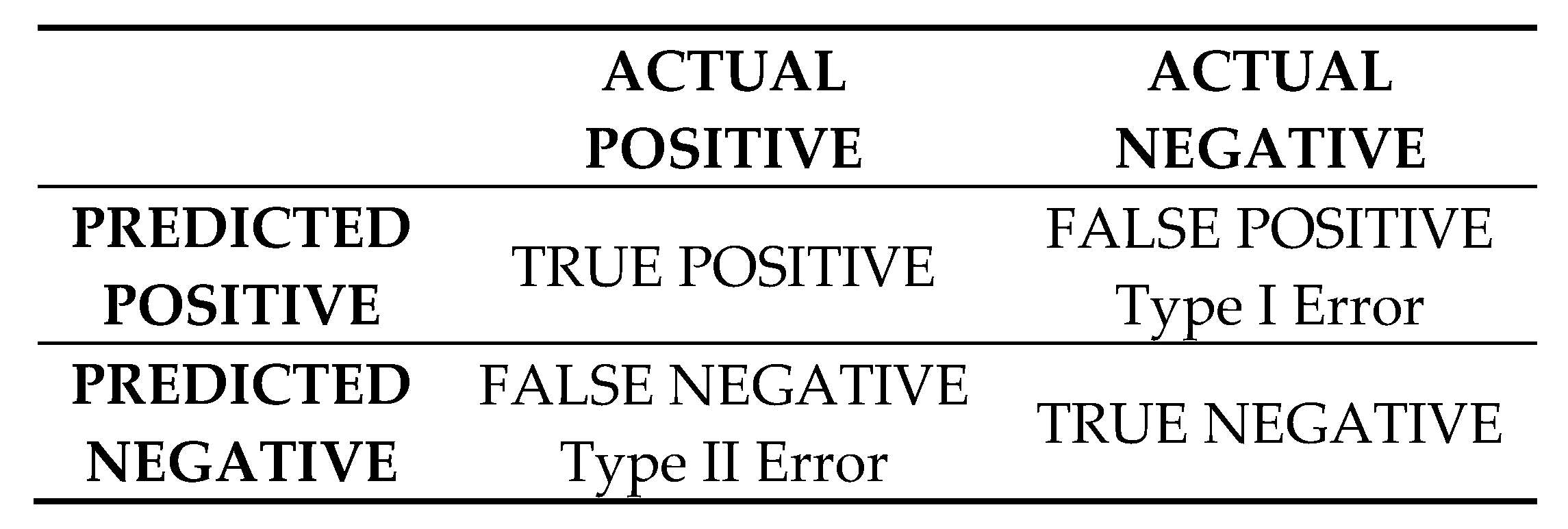
Guide for interpretation of confusion matrices.

References
- Saltikoff, E.; Friedrich, K.; Soderholm, J.; Lengfeld, K.; Nelson, B.; Becker, A.; Hollmann, R.; Urban, B.; Heistermann, M.; Tassone, C. An overview of using weather radar for climatological studies: Successes, challenges, and potential. Bull. Am. Meteorol. Soc. 2019, 100, 1739–1752. [Google Scholar] [CrossRef]
- Chilson, P.B.; Stepanian, P.M.; Kelly, J.F. Radar Aeroecology. In Aeroecology; Chilson, P.B., Frick, W.F., Kelly, J.F., Liechti, F., Eds.; Springer International Publishing: Cham, Switzerland, 2017; pp. 277–309. [Google Scholar] [CrossRef]
- Chilson, P.B.; Frick, W.F.; Kelly, J.F.; Liechti, F. (Eds.) Aeroecology; Springer: Cham, Switzerland, 2018. [Google Scholar] [CrossRef]
- Bauer, S.; Shamoun-Baranes, J.; Nilsson, C.; Farnsworth, A.; Kelly, J.F.; Reynolds, D.R.; Dokter, A.M.; Krauel, J.F.; Petterson, L.B.; Horton, K.G.; et al. The grand challenges of migration ecology that radar aeroecology can help answer. Ecography 2019, 42, 861–875. [Google Scholar] [CrossRef] [Green Version]
- Shamoun-Baranes, J.; Nilsson, C.; Bauer, S.; Chapman, J. Taking radar aeroecology into the 21st century. Ecography 2019, 42, 847–851. [Google Scholar] [CrossRef]
- Schmaljohann, H. Radar aeroecology—A missing piece of the puzzle for studying the migration ecology of animals. Ecography 2020. [Google Scholar] [CrossRef]
- Jungbluth, K.; Belles, J.; Schumacher, M. Velocity contamination of WSR-88D and wind profiler data due to migrating birds. In 27th Conference on Radar Meteorology; American Meteorological Society: Vail, CO, USA, 1995; pp. 9–13. [Google Scholar]
- Gauthreaux, S.A.; Mizrahi, D.S.; Belser, C.G. Bird migration and bias of WSR-88D wind estimates. Weather Forecast 1998, 13, 465–481. [Google Scholar] [CrossRef]
- Zhang, P.; Liu, S.; Xu, Q. Identifying doppler velocity contamination caused by migrating birds. Part I: Feature extraction and quantification. J. Atmos. Ocean. Technol. 2005, 22, 1105–1113. [Google Scholar] [CrossRef]
- Holleman, I.; Van Gasteren, H.; Bouten, W. Quality assessment of weather radar wind profiles during bird migration. J. Atmos. Ocean. Technol. 2008, 25, 2188–2198. [Google Scholar] [CrossRef] [Green Version]
- Zhang, P.; Xu, Q.; Ryzhkov, A.V. Identification of biological scatterers and radar data quality control. In 21st Conf. on Several Local Storms; American Meteorological Society: San Antonio, TX, USA, 2002; pp. 208–209. [Google Scholar]
- Rennie, S.J.; Curtis, M.; Peter, J.; Seed, A.W.; Steinle, P.J.; Wen, G. Bayesian echo classification for australian single-polarization weather radar with application to assimilation of radial velocity observations. J. Atmos. Ocean. Technol. 2015, 32, 1341–1355. [Google Scholar] [CrossRef]
- Dokter, A.M.; Farnsworth, A.; Fink, D.; Ruiz-Gutierrez, V.; Hochachka, W.M.; La Sorte, F.A.; Robinson, O.J.; Rosenberg, K.V.; Kelling, S. Seasonal abundance and survival of North America’s migratory avifauna determined by weather radar. Nat. Ecol. Evol. 2018, 2, 1603–1609. [Google Scholar] [CrossRef]
- Lin, T.; Winner, K.; Bernstein, G.; Mittal, A.; Dokter, A.M.; Horton, K.G.; Nilsson, C.; Van Doren, B.M.; Farnsworth, A.; La Sorte, F.A.; et al. MistNet: Measuring historical bird migration in the US using archived weather radar data and convolutional neural networks. Methods Ecol. Evol. 2019, 10, 1908–1922. [Google Scholar] [CrossRef]
- Rosenberg, K.V.; Dokter, A.M.; Blancher, P.J.; Sauer, J.R.; Smith, A.C.; Smith, P.A.; Stanton, J.C.; Panjabi, A.; Helft, L.; Parr, M.; et al. Decline of the North American avifauna. Science 2019, 366, 120–124. [Google Scholar] [CrossRef]
- Horton, K.G.; La Sorte, F.A.; Sheldon, D.; Lin, T.-Y.; Winner, K.; Bernstein, G.; Maji, S.; Hochachka, W.M.; Farnsworth, A. Phenology of nocturnal avian migration has shifted at the continental scale. Nat. Clim. Chang. 2020, 10, 63–68. [Google Scholar] [CrossRef]
- Chilson, P.B.; Frick, W.F.; Kelly, J.F.; Howard, K.W.; Larkin, R.P.; Diehl, R.H.; Westbrook, J.K.; Kelly, T.A.; Kunz, T.H. Partly cloudy with a chance of migration: Weather, radars, and aeroecology. Bull. Am. Meteorol. Soc. 2011, 93, 669–686. [Google Scholar] [CrossRef]
- Stepanian, P.M.; Horton, K.G.; Melnikov, V.M.; Zrnić, D.S.; Gauthreaux, S.A. Dual-polarization radar products for biological applications. Ecosphere 2016, 7, e01539. [Google Scholar] [CrossRef]
- Koistinen, J. Bird migration patterns on weather radars. Phys. Chem. Earth Part B Hydrol. Ocean. Atmos. 2000, 25, 1185–1193. [Google Scholar] [CrossRef]
- Martin, W.J.; Shapiro, A. Discrimination of bird and insect radar echoes in clear air using high-resolution radars. J. Atmos. Ocean. Technol. 2007, 24, 1215–1230. [Google Scholar] [CrossRef]
- Kessinger, C.; Ellis, S.; Van Andel, J. The radar echo classifier: A fuzzy logic algorithm for the WSR-88D. In 3rd Conference on Artificial Applications to the Environmental Science; American Meteorological Society: Long Beach, CA, USA, 2003; Available online: http://ams.confex.com/ams/pdfpapers/54946.pdf (accessed on 31 January 2020).
- Liu, S.; Xu, Q.; Zhang, P. Identifying Doppler Velocity Contamination Caused by Migrating Birds. Part II: Bayes Identification and Probability Tests. J. Atmos. Ocean. Technol. 2005, 22, 1114–1121. [Google Scholar] [CrossRef]
- Gauthreaux, S.A.; Livingston, J.W.; Belser, C.G. Detection and discrimination of fauna in the aerosphere using Doppler weather surveillance radar. Integr. Comp. Biol. 2008, 48, 12–23. [Google Scholar] [CrossRef] [Green Version]
- Van Gasteren, H.; Holleman, I.; Bouten, W.; Van Loon, E.; Shamoun-Baranes, J.; Van Loon, E.E. Extracting bird migration information from C-band Doppler weather radars. Ibis 2008, 150, 674–686. [Google Scholar] [CrossRef]
- Lakshmanan, V.; Zhang, J.; Howard, K. A technique to censor biological echoes in radar reflectivity data. J. Appl. Meteorol. Clim. 2010, 49, 453–462. [Google Scholar] [CrossRef] [Green Version]
- Bringi, V.N.; Chandrasekar, V. Polarimetric Doppler Weather Radar: Principles and Applications; Cambridge University Press: Cambridge, UK, 2001. [Google Scholar]
- Kumjian, M. Principles and applications of dual-polarization weather radar. Part I: Description of the polarimetric radar variables. J. Oper. Meteorol. 2013, 1, 226–242. [Google Scholar] [CrossRef]
- Park, H.S.; Ryzhkov, A.V.; Zrnic, D.S.; Kim, K.-E. The Hydrometeor classification algorithm for the polarimetric WSR-88D: Description and application to an MCS. Weather Forecast 2009, 24, 730–748. [Google Scholar] [CrossRef]
- Chandrasekar, V.; Keranen, R.; Lim, S.; Moisseev, D. Recent advances in classification of observations from dual polarization weather radars. Atmos. Res. 2013, 119, 97–111. [Google Scholar] [CrossRef]
- Schuur, T.; Ryzhkov, A.; Heinselman, P.; Zrnic, D.; Burgess, D.; Scharfenberg, K. Observations and Classification of Echoes with the Polarimetric WSR-88D Radar. In Report of the National Severe Storms Laboratory; National Severe Storms Laboratory: Norman, OK, USA, 2003; Volume 73069, p. 46. Available online: https://pdfs.semanticscholar.org/2d8e/5f5f5d26060726fa22b3700cfabbee043da.pdf (accessed on 5 November 2019).
- Ryzhkov, A.V.; Schuur, T.J.; Burgess, D.W.; Heinselman, P.L.; Giangrande, S.E.; Zrnic, D.S. The joint polarization experiment: Polarimetric rainfall measurements and hydrometeor classification. Bull. Am. Meteorol. Soc. 2005, 86, 809–824. [Google Scholar] [CrossRef] [Green Version]
- Lakshmanan, V.; Karstens, C.; Krause, J.; Tang, L. Quality Control of Weather Radar Data Using Polarimetric Variables. J. Atmos. Ocean. Technol. 2014, 31, 1234–1249. [Google Scholar] [CrossRef]
- Tang, L.; Zhang, J.; Langston, C.; Krause, J.; Howard, K.; Lakshmanan, V. A physically based precipitation–nonprecipitation radar echo classifier using polarimetric and environmental data in a real-time national system. Weather Forecast 2014, 29, 1106–1119. [Google Scholar] [CrossRef]
- Krause, J.M. A simple algorithm to discriminate between meteorological and nonmeteorological radar echoes. J. Atmos. Ocean. Technol. 2016, 33, 1875–1885. [Google Scholar] [CrossRef]
- Kilambi, A.; Fabry, F.; Meunier, V. A simple and effective method for separating meteorological from nonmeteorological targets using dual-polarization data. J. Atmos. Ocean. Technol. 2018, 35, 1415–1424. [Google Scholar] [CrossRef]
- Zrnic, D.; Ryzhkov, A. Observations of insects and birds with a polarimetric radar. IEEE Trans. Geosci. Remote. Sens. 1998, 36, 661–668. [Google Scholar] [CrossRef]
- Zhang, P.; Ryzhkov, A.; Zrnic, D. Detection of birds and insects using polarimetric radar observations. In 11th Conf. on Aviation, Range, and Aerospace Meteorology; CD-ROM P5.13; American Meteorological Society: Hyannis, MA, USA, 2004; pp. 897–901. Available online: https://www.semanticscholar.org/paper/Detection-of-Birds-and-Insects-Using-Polarimetric-Zhang/91cb7aff01d02c12f4f96d06350cf38820ffc068 (accessed on 31 January 2020).
- Zhang, P.F.; Ryzhkov, A.; Zrnic, D. Polarimetric prototype of the WSR-88D radar observation of birds and insects. In Preprints CD, 12th Conference on Aviation, Range, and Aerospace Meteorology; American Meteorological Society: Atlanta, GA, USA, 31 January 2006; Volume 28, Available online: https://www.semanticscholar.org/paper/P-6-.-4-POLARIMETRIC-PROTOTYPE-OF-THE-WSR-88-D-OF-Zhang-Ryzhkov/4c9b02aa1d88ed7f8c228dfb44212a30be02ee9a (accessed on 31 January 2020).
- Lang, T.J.; Rutledge, S.A.; Stith, J.L. Observations of quasi-symmetric echo patterns in clear air with the CSU–CHILL polarimetric radar. J. Atmos. Ocean. Technol. 2004, 21, 1182–1189. [Google Scholar] [CrossRef]
- Bachmann, S.; Zrnić, D. Spectral Density of Polarimetric Variables Separating Biological Scatterers in the VAD Display. J. Atmos. Ocean. Technol. 2007, 24, 1186–1198. [Google Scholar] [CrossRef] [Green Version]
- Melnikov, V.M.; Doviak, R.J.; Zrnic, D.S.; Stensrud, D.J. Mapping bragg scatter with a polarimetric WSR-88D. J. Atmos. Ocean. Technol. 2011, 28, 1273–1285. [Google Scholar] [CrossRef]
- Jiang, Y.; Xu, Q.; Zhang, P.; Nai, K.; Liu, L. Using WSR-88D polarimetric data to identify bird-contaminated doppler velocities. Adv. Meteorol. 2013, 2013, 1–13. [Google Scholar] [CrossRef] [Green Version]
- Melnikov, V.; Leskinen, M.; Koistinen, J. Doppler Velocities at orthogonal polarizations in radar echoes from insects and birds. Geosci. Remote Sens. Lett. IEEE 2014, 11, 592–596. [Google Scholar] [CrossRef]
- Melnikov, V.M.; Istok, M.J.; Westbrook, J.K. Asymmetric radar echo patterns from insects. J. Atmos. Ocean. Technol. 2015, 32, 659–674. [Google Scholar] [CrossRef]
- Stepanian, P.M.; Horton, K.G. Extracting migrant flight orientation profiles using polarimetric radar. IEEE Trans. Geosci. Remote Sens. 2015, 53, 6518–6528. [Google Scholar] [CrossRef]
- Buler, J.J.; Randall, L.A.; Fleskes, J.P.; Barrow, W.C.; Bogart, T.; Kluver, D. Mapping wintering waterfowl distributions using weather surveillance radar. PLoS ONE 2012, 7, e41571. [Google Scholar] [CrossRef] [Green Version]
- O’Neal, B.J.; Stafford, J.D.; Larkin, R.P. Waterfowl on weather radar: Applying ground-truth to classify and quantify bird movements. J. Field Ornithol. 2010, 81, 71–82. [Google Scholar] [CrossRef]
- Randall, L.A.; Diehl, R.H.; Wilson, B.C.; Barrow, W.C.; Jeske, C.W. Potential use of weather radar to study movements of wintering waterfowl. J. Wildl. Manag. 2011, 75, 1324–1329. [Google Scholar] [CrossRef]
- Horn, J.W.; Kunz, T.H. Analyzing NEXRAD doppler radar images to assess nightly dispersal patterns and population trends in Brazilian free-tailed bats (Tadarida brasiliensis). Integr. Comp. Biol. 2008, 48, 24–39. [Google Scholar] [CrossRef] [Green Version]
- Frick, W.F.; Stepanian, P.M.; Kelly, J.F.; Howard, K.W.; Kuster, C.M.; Kunz, T.H.; Chilson, P.B. Climate and weather impact timing of emergence of bats. PLoS ONE 2012, 7, e42737. [Google Scholar] [CrossRef] [Green Version]
- Van Den Broeke, M.S. Polarimetric radar observations of biological scatterers in hurricanes Irene (2011) and Sandy (2012). J. Atmos. Ocean. Tech. 2013, 30, 2754–2767. [Google Scholar] [CrossRef] [Green Version]
- Russell, K.R.; Gauthreaux, S.A. Use of weather radar to characterize movements of roosting purple martins. Wildl. Soc. Bull. 1998, 26, 5–16. [Google Scholar]
- Russell, K.R.; Mizrahi, D.S.; Gauthreaux, S.A., Jr. Large-scale mapping of purple martin pre-migratory roosts using WSR-88D weather surveillance radar. J. Field Ornithol. 1998, 69, 316–325. [Google Scholar]
- Gauthreaux, S.; Belser, C.G. Bird migration in the region of the Gulf of Mexico. In Proceedings of the 22nd International Ornithological Congress 1999, Durban, South Africa, 16–22 August 1998; pp. 1931–1947. [Google Scholar]
- Gauthreaux, S.A., Jr. Weather radar quantification of bird migration. BioScience 1970, 20, 17–19. [Google Scholar] [CrossRef]
- Gauthreaux, S.A.; Belser, C.G. Displays of bird movements on the WSR-88D: Patterns and quantification. Weather Forecast 1998, 13, 453–464. [Google Scholar] [CrossRef]
- Jehl, J.R., Jr.; Johansson, C. Autumnal migration of Eared Grebes (Podiceps nigricollis) through southwestern Wyoming: A key to assessing the size of the North American population. Western N. Am. Nat. 2002, 62, 9. Available online: https://scholarsarchive.byu.edu/wnan/vol62/iss3/9 (accessed on 5 November 2019).
- Jehl, J.R., Jr.; Day, K.; Schmidt, B. The spectacular (and hazardous) migration of Eared Grebes (Podiceps nigricollis) through southern Utah. N. Am. Birds 2012, 66, 2–9. [Google Scholar]
- Frank, M.; Conover, M. Factors influencing the fall migration of eared grebes from Great Salt Lake. In RESEARCH WEEK 2015; Utah State University: Logan, UT, USA, 2015; Available online: https://digitalcommons.usu.edu/researchweek/ResearchWeek2015/All2015/76/ (accessed on 5 November 2019).
- Williams, A.A.; Laird, N.F. Weather and eared grebe winter migration near the Great Salt Lake, Utah. Int. J. Biometeorol. 2018, 62, 433–447. [Google Scholar] [CrossRef]
- Breiman, L. Random forests. Mach. Learn. 2001, 45, 5–32. [Google Scholar] [CrossRef] [Green Version]
- Cutler, D.R.; Edwards, T.C., Jr.; Beard, K.H.; Cutler, A.; Hess, K.T.; Gibson, J.; Lawler, J.J. Random forests for classification in ecology. Ecology 2007, 88, 2783–2792. [Google Scholar] [CrossRef]
- R Core Team. R: A Language and Environment for Statistical Computing; R Foundation for Statistical Computing: Vienna, Austria, 2012; Available online: https://www.R-project.org/ (accessed on 31 January 2020).
- Chawla, N.V.; Bowyer, K.W.; Hall, L.O.; Kegelmeyer, W.P. SMOTE: Synthetic Minority Over-sampling Technique. J. Artif. Intell. Res. 2002, 16, 321–357. [Google Scholar] [CrossRef]
- Mueller, E.A.; Larkin, R.P. Insects observed using dual-polarization radar. J. Atmos. Ocean. Technol. 1985, 2, 49–54. [Google Scholar] [CrossRef] [Green Version]
- Achtemeier, G.L. The use of insects as tracers for “clear-air” boundary-layer studies by doppler radar. J. Atmos. Ocean. Tech. 1991, 8, 746–765. [Google Scholar] [CrossRef]
- Muller, B.; Mosher, F.; Herbster, C.; Brickhouse, A. Aviation bird hazard in NEXRAD dual polarization weather radar confirmed by visual observations. Int. J. Aviat. Aeronaut. Aerosp. 2015, 2, 1–6. [Google Scholar] [CrossRef] [Green Version]
- Chilson, C.; Avery, K.; McGovern, A.; Bridge, E.; Sheldon, D.; Kelly, J. Automated detection of bird roosts using NEXRAD radar data and Convolutional Neural Networks. Remote Sens. Ecol. Cons. 2019, 5, 20–32. [Google Scholar] [CrossRef]
- McCracken, G.F.; Gillam, E.H.; Westbrook, J.K.; Lee, Y.F.; Jensen, M.L.; Balsley, B.B. Brazilian free-tailed bats (Tadarida brasiliensis: Molossidae, Chiroptera) at high altitude: Links to migratory insect populations. Integr. Comp. Biol. 2008, 48, 107–118. [Google Scholar] [CrossRef] [Green Version]
- Jatau, P.; Melnikov, V. Bird detection algorithm for the WSR-88D radars. In Report on Radar Operations Center Memorandum of Understanding Task 14; University of Oklahoma, Cooperative Institute for Mesoscale Meteorological Studies: Norman, OK, USA, 2018. Available online: https://www.nssl.noaa.gov/publications/wsr88d_reports/BirdDetectionAlgorithm_2018.pdf (accessed on 5 November 2019).
- Zrnic, D.S.; Ryzhkov, A.V. Polarimetry for weather surveillance radars. Bull. Am. Meteorol. Soc. 1999, 80, 389–406. [Google Scholar] [CrossRef]
- Mirkovic, D.; Stepanian, P.M.; Kelly, J.F.; Chilson, P.B. Electromagnetic model reliably predicts radar scattering characteristics of airborne organisms. Sci. Rep. UK 2016, 6, 35637. [Google Scholar] [CrossRef]
- Shipley, J.R.; Kelly, J.F.; Frick, W.F. Toward integrating citizen science and radar data for migrant bird conservation. Remote Sens. Ecol. Cons. 2018, 4, 127–136. [Google Scholar] [CrossRef]
- Horton, K.G.; Van Doren, B.M.; La Sorte, F.A.; Fink, D.; Sheldon, D.; Farnsworth, A.; Kelly, J.F. Navigating north: How body mass and winds shape avian flight behaviours across a North American migratory flyway. Ecol. Lett. 2018, 21, 1055–1064. [Google Scholar] [CrossRef] [PubMed]
- Horton, K.G.; Van Doren, B.M.; La Sorte, F.A.; Cohen, E.B.; Clipp, H.L.; Buler, J.J.; Fink, D.; Kelly, J.F.; Farnsworth, A. Holding steady: Little change in intensity or timing of bird migration over the Gulf of Mexico. Glob. Chang. Boil. 2019, 25, 1106–1118. [Google Scholar] [CrossRef] [PubMed]
- Donnelly, J.P.; Naugle, D.E.; Collins, D.P.; Dugger, B.D.; Allred, B.W.; Tack, J.D.; Dreitz, V.J. Synchronizing conservation to seasonal wetland hydrology and waterbird migration in semi-arid landscapes. Ecosphere 2019, 10, e02758. [Google Scholar] [CrossRef]
- Meade, J.; Van Der Ree, R.; Stepanian, P.M.; Westcott, D.A.; Welbergen, J.A. Using weather radar to monitor the number, timing and directions of flying-foxes emerging from their roosts. Sci. Rep. 2019, 9, 10222. [Google Scholar] [CrossRef] [PubMed] [Green Version]
- Arnett, E.B.; Huso, M.M.; Schirmacher, M.R.; Hayes, J.P. Altering turbine speed reduces bat mortality at wind-energy facilities. Front. Ecol. Environ. 2010, 9, 209–214. [Google Scholar] [CrossRef] [Green Version]
- Schmaljohann, H.; Liechti, F.; Bächler, E.; Steuri, T.; Bruderer, B. Quantification of bird migration by radar —A detection probability problem. Ibis 2008, 150, 342–355. [Google Scholar] [CrossRef]
- Horton, K.G.; Shriver, W.G.; Buler, J.J. A comparison of traffic estimates of nocturnal flying animals using radar, thermal imaging, and acoustic recording. Ecol. Appl. 2015, 25, 390–401. [Google Scholar] [CrossRef]
- Drake, V.A. Distinguishing target classes in observations from vertically pointing entomological radars. Int. J. Remote Sens. 2016, 37, 3811–3835. [Google Scholar] [CrossRef]
- Wang, R.; Hu, C.; Fu, X.; Long, T.; Zeng, T. Micro-Doppler measurement of insect wing-beat frequencies with W-band coherent radar. Sci. Rep. 2017, 7, 1396. [Google Scholar] [CrossRef] [Green Version]
- Radhakrishna, B.; Fabry, F.; Kilambi, A. Fuzzy logic algorithms to identify birds, precipitation, and ground clutter in s-band radar data using polarimetric and nonpolarimetric variables. J. Atmos. Ocean. Technol. 2019, 36, 2401–2414. [Google Scholar] [CrossRef]
- Van Gasteren, H.; Krijgsveld, K.L.; Klauke, N.; Leshem, Y.; Metz, I.C.; Skakuj, M.; Sorbi, S.; Schekler, I.; Shamoun-Baranes, J. Aeroecology meets aviation safety: Early warning systems in Europe and the Middle East prevent collisions between birds and aircraft. Ecography 2019, 42, 899–911. [Google Scholar] [CrossRef]
- Leskinen, M.; Markkula, I.; Koistinen, J.; Pylkkö, P.; Ooperi, S.; Siljamo, P.; Ojanen, H.; Raiskio, S.; Tiilikkala, K. Pest insect immigration warning by an atmospheric dispersion model, weather radars and traps. J. Appl. Entomol. 2011, 135, 55–67. [Google Scholar] [CrossRef] [Green Version]
- Gauthreaux, S.A.; Belser, C.G. Radar ornithology and biological conservation. Auk 2003, 120, 266–277. [Google Scholar] [CrossRef]
- Hüppop, O.; Ciach, M.; Diehl, R.; Reynolds, D.R.; Stepanian, P.M.; Menz, M.H.M. Perspectives and challenges for the use of radar in biological conservation. Ecography 2019, 42, 912–930. [Google Scholar] [CrossRef]
- Bauer, S.; Chapman, J.W.; Reynolds, D.R.; Alves, J.A.; Dokter, A.M.; Menz, M.M.H.; Sapir, N.; Ciach, M.; Pettersson, L.B.; Kelly, J.F.; et al. From agricultural benefits to aviation safety: Realizing the potential of continent-wide radar networks. Bioscience 2017, 67, 912–918. [Google Scholar] [CrossRef]
- Zrnic, D.S.; Kimpel, J.F.; Forsyth, D.E.; Shapiro, A.; Crain, G.; Ferek, R.; Heimmer, J.; Benner, W.; McNellis, T.J.; Vogt, R.J. Agile-beam phased array radar for weather observations. Bull. Am. Meteorol. Soc. 2007, 88, 1753–1766. [Google Scholar] [CrossRef]
- Zhang, G.; Mahale, V.N.; Putnam, B.J.; Qi, Y.; Cao, Q.; Byrd, A.D.; Bukovcic, P.; Zrnic, D.S.; Gao, J.; Xue, M.; et al. Current status and future challenges of weather radar polarimetry: Bridging the gap between radar meteorology/hydrology/engineering and numerical weather prediction. Adv. Atmos. Sci. 2019, 36, 571–588. [Google Scholar] [CrossRef] [Green Version]
- Wen, G.; Protat, A.; Xiao, H. An objective prototype-based method for dual-polarization radar clutter identification. Atmosphere 2017, 8, 72. [Google Scholar] [CrossRef] [Green Version]
- Melnikov, V.; Zrnic, D.S. Observations of convective thermals with weather radar. J. Atmos. Ocean. Technol. 2017, 34, 1585–1590. [Google Scholar] [CrossRef]
- Balakrishnan, N.; Zrnic, D.S. Use of polarization to characterize precipitation and discriminate large hail. J. Atmos. Sci. 1990, 47, 1525–1540. [Google Scholar] [CrossRef]
- Browning, K.A.; Nicol, J.C.; Marsham, J.H.; Rogberg, P.; Norton, E.G. Layers of insect echoes near a thunderstorm and implications for the interpretation of radar data in terms of airflow. Q. J. R. Meteorol. Soc. 2011, 137, 723–735. [Google Scholar] [CrossRef]
- Buban, M.S.; Ziegler, C.L.; Rasmussen, E.N.; Richardson, Y.P. The dryline on 22 May 2002 during IHOP: Ground-radar and in situ data analyses of the dryline and boundary layer evolution. Mon. Weather Rev. 2007, 135, 2473–2505. [Google Scholar] [CrossRef]
- Wilson, J.W.; Weckwerth, T.M.; Vivekanandan, J.; Wakimoto, R.M.; Russell, R.W. Boundary layer clear-air radar echoes: Origin of echoes and accuracy of derived winds. J. Atmos. Ocean. Technol. 1994, 11, 1184–1206. [Google Scholar] [CrossRef] [Green Version]
- Bachmann, S.; Zrnic, D. Spectral polarimetry for identifying and separating mixed biological scatters. In Proceedings of the 32nd International Conference on Radar Meteorology, Albuquerque, NM, USA, 27 October 2005; P9R.5. Available online: https://www.semanticscholar.org/paper/Spectral-polarimetry-for-identifing-and-separating-Bachmann/fa7698e7e4317b8698a1d83a1777c95f0c41c1d1 (accessed on 31 January 2020).
- Ryzhkov, A.V.; Janish, J.M.; Schuur, T.J.; Zhang, P.; Elmore, K.L. Dual-polarization radar as a tool for operational identification of different types of meteorological and non-meteorological targets. In Proceedings of the 13th Conference on Applied Climatology and the 10th Conference on Aviation, Range, and Aerospace Meteorology, Portland, OR, USA, 13–16 May 2002; pp. 104–107. [Google Scholar]
- Vaughn, C.R. Birds and insects as radar targets: A review. Proc. IEEE 1985, 73, 205–227. [Google Scholar] [CrossRef]
- Zrnic, V.M.D.S.; Zrnic, D.; Melnikov, V.; Ryzhkov, A. Use of backscatter differential phase in weather surveillance radars. In Proceedings of the 2004 IEEE International Geoscience and Remote Sensing Symposium, Anchorage, AK, USA, 20–24 September 2004; Volume 1, pp. 456–458. [Google Scholar] [CrossRef]
Figure 1.
Array of histograms showing the distribution of values of six radar variables for seven types of scatterer.
Figure 1.
Array of histograms showing the distribution of values of six radar variables for seven types of scatterer.

Figure 2.
Non-metric multidimensional scaling (MDS) of confusion matrix values from Table 5a. Less distance between classes indicates greater similarity. Vertebrates are colored green, arthropods red, and precipitation blue.
Figure 2.
Non-metric multidimensional scaling (MDS) of confusion matrix values from Table 5a. Less distance between classes indicates greater similarity. Vertebrates are colored green, arthropods red, and precipitation blue.

Figure 3.
Variable importance indices generated by separate binary RF models trained to distinguish between a focal biological class (shown) and a class that drew samples equitably from all remaining classes combined (the exception being results for the CA model which distinguished between vertebrates and arthropods; see Table 3). Values shown indicate the importance of a variable in partitioning the data into the defined classes. Each of the six features is labeled and identified by a different color. The figure is divided into output from low- (left), moderate- (center), and high- (right) aggregation models. With the exception of the EAGR model, all binary models were based on identical sample sizes balanced between the two classes. The EAGR model was also balanced between the classes but based on fewer samples, so importance metrics for this model were scaled up proportionately based on those of the other binary models.

Figure 4.
The proportion of radar data retained varied inversely with the classification probability of resolution volumes. Data from a single 0.5° elevation sweep on 13 July 2014 at 10:33 UT from the WSR-88D radar in Columbia, SC (KCAE) classified according to three RF models built using different levels of aggregation. (These data were excluded from RF model training or testing.) The panel of sweeps above-left is dominated by purple martins (green), precipitation (blue), and presumed insects (red), and shows the distribution of resolution volumes exceeding different classification probability thresholds. The left column of sweeps shows the majority classification and middle and right columns show resolution volumes retained with probabilities of classification ≥0.95 and ≥0.99, respectively. Resolution volumes below these thresholds were dropped and are shown as white space. For each level of aggregation, the distribution of resolution volumes on the left represents three points along their respective curves to the right, as shown in blue for precipitation and in green, from top to bottom, for biological, vertebrates, and purple martins.

Figure 5.
Areas where scatterer types mixed within resolution volumes reduced the probability of class membership and/or led to misclassification. Data from a single 0.5° elevation sweep on 9 May 2017 at 04:57 UT from the WSR-88D radar in Romeoville, IL (KLOT) classified according to two RF models built using high and low levels of aggregation. The panel of sweeps shows the distribution of resolution volumes at two different probabilistic classification thresholds, the majority classification, which depended on the number of classes (left), and those with probability of classification ≥0.95 (upper right; lower right intentionally left blank). Resolution volumes below this threshold were dropped and are shown as white space, often bordering precipitation. Pixels that did not have velocity data were not classified by our models and are colored gray.

Table 1.
Scatterer types included in classification training data.
| Aggregation 1 | Sample Size 2 (RV/Sweeps/Radars) | Description | ||
|---|---|---|---|---|
| Low | Medium | High | ||
| Trans-gulf migrants (TGMI) | vertebrates | biological | 1,522,978/30/5 | Songbird-dominated migration over open water of the Gulf |
| Purple martins (PUMA) | vertebrates | biological | 47,620/13/11 | Morning roost departure |
| Waterfowl (WRFL) | vertebrates | biological | 162,870/11/4 | Ducks, geese, some cranes; migratory departure |
| Eared grebes (EAGR) | vertebrates | biological | 21,815/14/1 | Migratory departure nearly due south out of Great Salt Lake |
| Free-tailed bats (FTBA) | vertebrates | biological | 49,049/11/5 | Evening roost departure |
| Aerial plankton (ISCT) | arthropods | biological | 1,208,953/15/11 | Broad-front diurnal insect movement |
| Mayflies, midges (SWRM) | arthropods | biological | 98,354/21/3 | Mating swarms |
| Precipitation (PRCP) | precipitation | precipitation | 1,374,235/15/12 | Light to moderate rain |
1 Degree of aggregation refers to how types of scatterers were grouped for different analyses. 2 Number of resolution volumes (RV), number of 0.5° sweeps, and number of different radars.
Table 2.
Random forest models executed for this project broken down by their level of aggregation, classes in the model, and discriminating variables.
Table 2.
Random forest models executed for this project broken down by their level of aggregation, classes in the model, and discriminating variables.
| Aggregation | Classes | Variables | Description/Notes |
|---|---|---|---|
| High | biological–precipitation | ZH, Vr, σV, ZDR, ρHV, ΦDP | aggregates six biological classes |
| Medium | vertebrates–arthropods–precipitation | ZH, Vr, σV, ZDR, ρHV, ΦDP | aggregates 4 vertebrate and 2 arthropod classes |
| vertebrates–arthropods–precipitation | ZH, Vr, σV | as above, original variables only | |
| vertebrates–arthropods–precipitation | ZDR, ρHV, ΦDP | as above, polarimetry variables only | |
| vertebrates–arthropods | ZH, Vr, σV, ZDR, ρHV, ΦDP | as above, sans precipitation | |
| vertebrates–other | ZH, Vr, σV, ZDR, ρHV, ΦDP | “other” equally under-samples arthropods and precipitation | |
| arthropods–other | ZH, Vr, σV, ZDR, ρHV, ΦDP | “other” equally under-samples vertebrates and precipitation | |
| precipitation–other | ZH, Vr, σV, ZDR, ρHV, ΦDP | “other” equally under-samples vertebrates and arthropods | |
| Low | SWRM–ISCT–WRFL–TGMI–PUMA–FTBA–PRCP | ZH, Vr, σV, ZDR, ρHV, ΦDP | biological classes considered together in multinomial models |
| SWRM–ISCT–WRFL–TGMI–PUMA–FTBA–PRCP | ZH, Vr, σV | as above, original variables only | |
| SWRM–ISCT–WRFL–TGMI–PUMA–FTBA–PRCP | ZDR, ρHV, ΦDP | as above, polarimetry variables only | |
| TGMI–ISCT | ZH, Vr, σV, ZDR, ρHV, ΦDP | common discrimination problem | |
| Scatterer 1–other | ZH, Vr, σV, ZDR, ρHV, ΦDP | “other” equally under-samples non-SWRM classes | |
| EAGR–other | ZH, Vr, σV, ZDR, ρHV, ΦDP, AZ, RA | as above, includes azimuth (AZ) and range (RA) as variables |
1 Refers to each bioscatterer type—SWRM, ISCT, WRFL, TGMI, PUMA, FTBA, EAGR—classified individually against ‘other’ in seven separate models.
Table 3.
Classification results of binary RF models, each focused on a specific scatterer type at high and moderate levels of aggregation. Values are percent of the total out-of-bag samples assigned to that class. “Taxa” below refers to the corresponding focal class, vertebrates or arthropods, in their respective confusion matrices. Percent true positive classifications are highlighted and bold. “Other” is a class of resolution cells equally represented by the non-focal classes, i.e., the non-vertebrate classes and precipitation or the non-arthropod classes and precipitation. Interpretation of confusion matrices can be found in Figure A3.
| a. High Aggregation | ||
| Biological | Precip | |
| Biological | 98.7 | 1.3 |
| Precip | 2.2 | 97.8 |
| b. Medium Aggregation | ||
| Taxa | Other | |
| Vertebrates | 94.8 | 5.2 |
| Other | 6.8 | 93.2 |
| Arthropods | 93.5 | 6.5 |
| Other | 5.4 | 94.6 |
| Vertebrates | Arthropods | |
| Vertebrates | 94.3 | 5.7 |
| Arthropods | 7.3 | 92.7 |
Table 4.
Classification results of seven binary RF models, each focused on a specific scatterer type at the lowest level of aggregation. Values are percent of the total out-of-bag samples assigned to that class. “Taxa” refers to the corresponding focal class (e.g., ISCT, TGMI) in each confusion matrix. Percent true positive classifications are highlighted and bold. “Other” is a class of resolution cells equally represented by all non-focal classes.
| Taxa | Other | |
|---|---|---|
| ISCT | 93.0 | 7.0 |
| Other | 5.7 | 94.3 |
| FTBA | 92.2 | 7.8 |
| Other | 8.2 | 91.8 |
| SWRM | 95.2 | 4.8 |
| Other | 3.9 | 96.1 |
| TGMI | 86.9 | 13.1 |
| Other | 19.0 | 81.0 |
| PUMA | 90.5 | 9.5 |
| Other | 18.2 | 81.8 |
| WRFL | 87.7 | 12.3 |
| Other | 12.7 | 87.3 |
| TGMI | 95.8 | 4.2 |
| ISCT | 6.1 | 93.9 |
Table 5.
Seven-class multinomial RF model results showing classification of validated scatterers in the non-training set. Values are percent of the total out-of-bag samples assigned to that class. Percent classification error is summed to the right. Error contribution (EC) is the median percent error contributed by that class across all classifications. Results are given for models based on three different variable combinations; (a) all six variables, (b) three legacy variables (ZH, Vr, σV), and (c) three polarimetry variables (ZDR, ρHV, ΦDP). For each model, the true positive (in bold) and highest false positive results are highlighted by the same color.
| a. All variables | ||||||||
| SWRM | ISCT | WRFL | TGMI | PUMA | FTBA | PRCP | Error | |
| SWRM | 90.3 | 3.9 | 1.8 | 1.4 | 1.8 | 0.4 | 0.5 | 9.7 |
| ISCT | 2.1 | 87.9 | 0.7 | 1.5 | 5.8 | 1.9 | 0.1 | 12.1 |
| WRFL | 2.4 | 1.5 | 71.6 | 11.4 | 9.9 | 2.0 | 1.2 | 28.4 |
| TGMI | 2.1 | 2.4 | 11.7 | 59.4 | 18.7 | 5.2 | 0.5 | 40.6 |
| PUMA | 1.5 | 5.6 | 4.5 | 10.3 | 68.8 | 8.7 | 0.5 | 31.2 |
| FTBA | 1.0 | 2.6 | 1.2 | 3.7 | 8.9 | 82.5 | 0.1 | 17.5 |
| PRCP | 0.6 | 0.2 | 1.7 | 0.6 | 0.7 | 0.1 | 96.2 | 3.8 |
| EC | 1.8 | 2.5 | 1.7 | 2.6 | 7.3 | 1.9 | 0.5 | |
| b. Legacy Variables | ||||||||
| SWRM | ISCT | WRFL | TGMI | PUMA | FTBA | PRCP | Error | |
| SWRM | 72.3 | 6.9 | 1.3 | 2.3 | 2.6 | 8.4 | 6.1 | 27.7 |
| ISCT | 0.9 | 72.7 | 0.7 | 2.7 | 8.1 | 14.8 | 0.1 | 27.3 |
| WRFL | 9.8 | 4.2 | 42.8 | 14.3 | 8.9 | 9.6 | 10.5 | 57.2 |
| TGMI | 7.1 | 7.0 | 11.5 | 36.9 | 13.5 | 21.9 | 2.2 | 63.1 |
| PUMA | 1.9 | 17.7 | 1.7 | 7.4 | 37.2 | 32.4 | 1.7 | 62.8 |
| FTBA | 6.4 | 12.2 | 1.3 | 2.9 | 11.9 | 63.2 | 2.1 | 36.8 |
| PRCP | 23.9 | 0.6 | 7.5 | 3.2 | 3.6 | 5.5 | 55.7 | 44.3 |
| EC | 6.8 | 7.0 | 1.5 | 3.0 | 8.5 | 12.2 | 2.2 | |
| c. Dual-Pol Variables | ||||||||
| SWRM | ISCT | WRFL | TGMI | PUMA | FTBA | PRCP | Error | |
| SWRM | 60.0 | 23.1 | 7.6 | 3.5 | 1.4 | 3.4 | 1.1 | 40.0 |
| ISCT | 15.6 | 65.0 | 10.3 | 4.2 | 3.0 | 1.1 | 0.9 | 35.0 |
| WRFL | 5.3 | 6.8 | 53.5 | 13.4 | 13.2 | 6.7 | 1.2 | 46.5 |
| TGMI | 4.9 | 6.4 | 28.4 | 32.6 | 16.8 | 6.7 | 4.2 | 67.4 |
| PUMA | 3.0 | 8.6 | 32.7 | 17.7 | 27.7 | 8.9 | 1.5 | 72.3 |
| FTBA | 4.4 | 3.1 | 11.1 | 8.0 | 3.7 | 69.5 | 0.2 | 30.5 |
| PRCP | 0.9 | 0.3 | 1.6 | 2.0 | 0.9 | 0.1 | 94.2 | 5.8 |
| EC | 4.6 | 6.6 | 10.7 | 6.1 | 3.3 | 5.0 | 1.1 | |
Table 6.
Three-class multinomial RF model results showing classification of validated scatterers in the non-training set. Values are percent of the total out-of-bag samples assigned to that class. Results are given for models based on three different variable combinations, (a) all six variables, (b) three legacy variables (ZH, Vr, σV), and (c) three polarimetry variables (ZDR, ρHV, ΦDP). Percent true positive classifications are highlighted and bold. Percent classification error is summed to the right.
| a. All variables | ||||
| Vertebrates | Arthropods | Precip. | Error | |
| Vertebrates | 93.1 | 5.6 | 1.3 | 6.9 |
| Arthropods | 6.8 | 92.7 | 0.5 | 7.3 |
| Precip. | 1.7 | 0.7 | 97.5 | 2.5 |
| b. Legacy variables | ||||
| Vertebrates | Arthropods | Precip. | Error | |
| Vertebrates | 76.4 | 14.0 | 9.6 | 23.6 |
| Arthropods | 20.3 | 66.7 | 13.0 | 33.3 |
| Precip. | 14.5 | 11.4 | 74.1 | 25.9 |
| c. Dual-pol variables | ||||
| Vertebrates | Arthropods | Precip. | Error | |
| Vertebrates | 84.0 | 13.2 | 2.8 | 16.0 |
| Arthropods | 14.9 | 83.7 | 1.4 | 16.3 |
| Precip. | 3.1 | 1.2 | 95.7 | 4.3 |
Table 7.
Classification results of EAGR binary RF models that differed by the addition of azimuth and range as spatially constraining variables. Values are percent of the total out-of-bag samples assigned to that class. Percent true positive classifications are highlighted and bold. “Other” is a class of resolution cells equally represented by all non-focal classes.
| EAGR | Other | |
| EAGR | 97.5 | 2.5 |
| Other | 6.1 | 93.9 |
| EAGR | Other | |
| EAGR | 99.8 | 0.2 |
| Other | 0.3 | 99.7 |
© 2020 by the authors. Licensee MDPI, Basel, Switzerland. This article is an open access article distributed under the terms and conditions of the Creative Commons Attribution (CC BY) license (http://creativecommons.org/licenses/by/4.0/).
Share and Cite
MDPI and ACS Style
Gauthreaux, S.; Diehl, R. Discrimination of Biological Scatterers in Polarimetric Weather Radar Data: Opportunities and Challenges. Remote Sens. 2020, 12, 545. https://0-doi-org.brum.beds.ac.uk/10.3390/rs12030545
AMA Style
Gauthreaux S, Diehl R. Discrimination of Biological Scatterers in Polarimetric Weather Radar Data: Opportunities and Challenges. Remote Sensing. 2020; 12(3):545. https://0-doi-org.brum.beds.ac.uk/10.3390/rs12030545
Chicago/Turabian StyleGauthreaux, Sidney, and Robert Diehl. 2020. "Discrimination of Biological Scatterers in Polarimetric Weather Radar Data: Opportunities and Challenges" Remote Sensing 12, no. 3: 545. https://0-doi-org.brum.beds.ac.uk/10.3390/rs12030545
Note that from the first issue of 2016, this journal uses article numbers instead of page numbers. See further details here.