Comparison of True-Color and Multispectral Unmanned Aerial Systems Imagery for Marine Habitat Mapping Using Object-Based Image Analysis

Abstract

The use of unmanned aerial systems (UAS) over the past years has exploded due to their agility and ability to image an area with high-end products. UAS are a low-cost method for close remote sensing, giving scientists high-resolution data with limited deployment time, accessing even the most inaccessible areas. This study aims to produce marine habitat mapping by comparing the results produced from true-color RGB (tc-RGB) and multispectral high-resolution orthomosaics derived from UAS geodata using object-based image analysis (OBIA). The aerial data was acquired using two different types of sensors—one true-color RGB and one multispectral—both attached to a UAS, capturing images simultaneously. Additionally, divers’ underwater images and echo sounder measurements were collected as in situ data. The produced orthomosaics were processed using three scenarios by applying different classifiers for the marine habitat classification. In the first and second scenario, the k-nearest neighbor (k-NN) and fuzzy rules were applied as classifiers, respectively. In the third scenario, fuzzy rules were applied in the echo sounder data to create samples for the classification process, and then the k-NN algorithm was used as the classifier. The in situ data collected were used as reference and training data. Additionally, these data were used for the calculation of the overall accuracy of the OBIA process in all scenarios. The classification results of the three scenarios were compared. Using tc-RGB instead of multispectral data provides better accuracy in detecting and classifying marine habitats when applying the k-NN as the classifier. In this case, the overall accuracy was 79%, and the Kappa index of agreement (KIA) was equal to 0.71, which illustrates the effectiveness of the proposed approach. The results showed that sub-decimeter resolution UAS data revealed the sub-bottom complexity to a large extent in relatively shallow areas as they provide accurate information that permits the habitat mapping in extreme detail. The produced habitat datasets are ideal as reference data for studying complex coastal environments using satellite imagery.

1. Introduction

Coastal zones are among the most populated and most productive areas in the world, offering a variety of habitats and ecosystem services. The European Commission highlights the importance of coastal zone management with the application of different policies and related activities, which were adopted through the joint initiatives of Maritime Spatial Planning and Integrated Coastal Management [1]. The aim is to promote sustainable growth of maritime and coastal activities and to use coastal and marine resources sustainably. Several other environmental policies are included in this initiative, like the Marine Strategy Framework Directive, the Climate Change Adaptation, and the Common Fisheries Policy [1]. Marine habitats have important ecological and regulatory functions and should be monitored in order to detect ecosystem changes [2,3]. Thus, habitat mapping is a prime necessity for environmental planning and management [4,5]. The continued provision of updated habitat maps has a decisive contribution to the design and coordination of relevant actions, the conservation of natural resources, and the monitoring of changes caused by natural disasters or anthropogenic effects [6]. Habitat maps are in critical demand, raising increasing interest among scientists monitoring sensitive coastal areas. The significance of coastal habitat mapping lies in the need to prevent anthropogenic interventions and other factors that affect the coastal environment [7]. Habitat maps are spatial representations of natural discrete seabed areas associated with particular species, communities, or co-occurrences. These maps can reflect the nature, distribution, and extent of disparate natural environments and can predict the species distribution [8].

Remote sensing has long-been identified as a technology capable of supporting the development of coastal zone monitoring and habitat mapping over large areas [1,9]. These processes require multitemporal data, either from satellites or from unmanned aerial systems (UAS). The availability of very high-resolution orthomosaics presents increasing interest, as it provides to scientists and relevant stakeholders detailed information for understanding coastal dynamics and implementing environmental policies [6,10,11,12,13]. However, the use of high-resolution orthomosaics created from UAS data is expected to improve mapping accuracy. This improvement is due to the high-spatial resolution of the orthomosaics less than 30 cm.

The increasing demand of detailed maps for monitoring the coastal areas requires automatic algorithms and techniques. Object-based image analysis (OBIA) is an object-based analysis of remote sensing imagery that uses automated methods to partition imagery into meaningful image-objects and generate geographic information in a GIS-ready format, from which new knowledge can be obtained [6,14,15].

In literature, there are several studies presenting the combination of OBIA with UAS imagery in habitat mapping. Husson et al. 2016 demonstrated an automated classification of nonsubmerged aquatic vegetation using OBIA and tested two classification methods (threshold classification and random forest) using eCognition® to true-color UAS images [2]. Furthermore, the produced automated classification results were compared to those of the manual mapping. In another study, Husson et al. 2017 combined height data from a digital surface model (DSM) created from overlapping UAS images with the spectral and textural features from the UAS orthomosaic to test if classification accuracy can be further improved [3]. They proved that the use of DSM-derived height data increased significantly the overall accuracy by 4%–21% for growth forms and 3%–30% for the dominant class. They concluded that height data have a significant potential to efficiently increase the accuracy of the automated classification of nonsubmerged aquatic vegetation.

Ventura et al. 2016 [16] carried out habitat mapping using a low-cost UAS. They tried to locate coastal areas suitable for fish nursery in the study area using UAS data and applying three different classification approaches. UAS data were collected using a video camera, and the acquired video was converted into a photo sequence, resulting in the orthomosaic of the study area. In this study, three classifications were performed using three different methods: (i) maximum likelihood in ArcGIS 10.4, (ii) extraction and classification of homogeneous objects (ECHO) in MultiSpec 3.4, and (iii) OBIA in eCognition Developer 8.7, with an overall accuracy of 78.8%, 80.9%, and 89.01%, respectively [16]. In a subsequent study, Ventura et al. 2018 [12] referred to the island of Giglio in Central Italy, where they carried out habitat mapping in three different coastal environments. Using OBIA and the nearest neighbor algorithm as classifiers, four different classifications were applied to identify Posidonia Oceanica meadows, nurseries for juvenile fish, and biogenic reefs with overall accuracies of 85%, 84%, and 80%, respectively. In another study, Makri D. et al. 2018 [17], a multiscale image analysis methodology was performed at Livadi Beach located on Folegandros Island, Greece. Landsat-8 and Sentinel-2 imagery were georeferenced, and atmospheric and water columns were corrected and analyzed using OBIA. As in situ data, high-resolution UAS data were collected. These data were used, as well in the classification and accuracy assessment. The nearest neighbor algorithm and fuzzy logic rules were used as classifiers. In this study, the overall accuracy was calculated to be 53% for Landsat-8 and 66% for Sentinel- 2 imagery. Duffy J. et al. 2018 [18] studied the creation of seagrass maps in Wales using a light drone for data acquisition. Three different classification methods were examined using the R 3.3.1 software [19]. The first classification performed unsupervised classification to true-color RGB (tc-RGB) data implemented in the ‘RStoolbox’ package [20,21]. The second classification was realized using tc-RGB data in combination with the texture of the image. Finally, the third classification was based on the object-based image analysis in the Geographic Resources Analysis Support System (GRASS) 7.0 software [22,23]. The accuracy of the classifications was based on the root mean square deflection (RMSD), and the results showed that unsupervised classifications had better accuracy in the seagrass coverage in comparison with the object-based image analysis method. These studies demonstrate that UAS data can provide critical information regarding the OBIA classification process and have the potential to increase classification accuracy in habitat mapping.

This study aimed to investigate the use of an automated classification approach by applying OBIA to high-resolution UAS multispectral and true-color RGB imagery for marine habitat mapping. Based on orthorectified image mosaics (here called UAS orthomosaics), we perform OBIA to map marine habitats in areas with varying levels of habitat complexity on the coastal zone. For the first time, UAS tc-RGB and multispectral orthomosaics were processed following OBIA methodology, and the classification results were compared by applying different classifiers for marine habitat mapping. Furthermore, the performance of the same classifier when applied to different orthomosaics (tc-RGB and multispectral) was examined in terms of accuracy and efficiency in classifications for marine habitat mapping. The object-based image analysis was performed using as classifiers the k-nearest neighbor algorithm and fuzzy logic rules. The validity of the produced maps was estimated using the overall accuracy and the Kappa index coefficient. Furthermore, divers’ photos and roughness information derived from echo sounders were used as in situ data to assess the final results. Finally, we compared the results between multispectral and true-color UAS data for the automatic classification habitat mapping and analyzed them concerning the classification accuracy.

2. Materials and Methods

2.1. Study Area

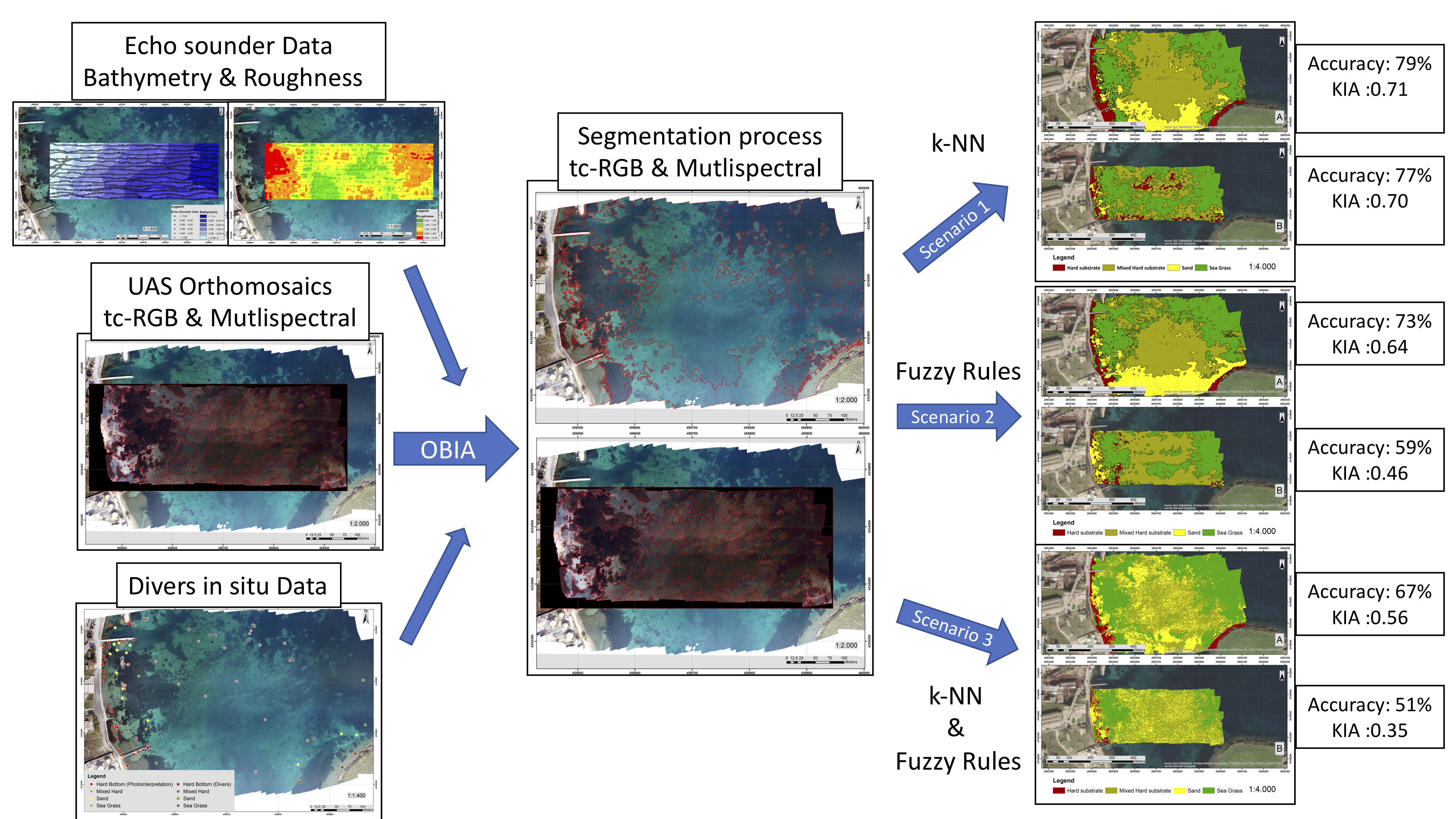
The area used in this study is located in the coastal zone of Pamfila Beach on Lesvos Island, Greece (Figure 1). Lesvos is the third-largest Greek island, having 320 km of coastline, located in the Northeastern Aegean Sea. Pamfila Beach lies in the eastern part of Lesvos Island (39° 9′30.17″ N, 26° 31′53.35″ E), and the islet called Pamfilo is in front of the beach. Furthermore, an olive press and a petroleum storage facility are located close to the beach. This combination creates a unique marine environment; thus, sea meadows mapping is in critical demand for this area. There are four main marine habitats: hard bottom, sand, seagrass, and mix hard substrate. The hard substrate appears in the intertidal and the very shallow zone (0 to 1.5 m). The sand class covers mainly the southern part of the study area, and the mixed hard substrate is mainly located in the center of the study area, at depths of about 2.5 to 6.5 m. The seagrass class (Posidonia Oceanica) is dominant in the area and is presented at a depth of about 1.5 to 3.5 m. and 6.5 to 7.9 m.

2.2. Classification Scheme

Four categories of the European Nature Information System (EUNIS, 2007) habitat classification list were selected for the classification process: (i) hard substrate, (ii) seagrass, (iii) sand, and (iv) mixed hard substrate. Due to the high resolution of orthomosaics (2 to 5 cm), we assume that each pixel is covered 100% by its class; i.e., a pixel is categorized as seagrass when it is covered 100%. The four classes selected as the predominant classes were previously known from local observations and studies. The seagrass class (code A5.535)—namely, Posidonia Oceanica beds—is characterized by the presence of the marine seagrass (phanerogam) Posidonia Oceanica. This habitat is an endemic Mediterranean species creating natural formations called Posidonia meadows. These meadows are found at depths of 1 to 50 m. The sand class (code A5.235) is encountered in very shallow water where the sea bottom is characterized by fine sand, usually with homogeneous granulometry and of terrigenous origin. The class of hard substrate (code A3.23) is characterized by the presence of many photophilic algae covering hard bottoms in moderately exposed areas. Finally, the mixed hard substrate class is considered as an assemblage of sand, seagrass, and dead seagrass leaves covering a hard substrate.

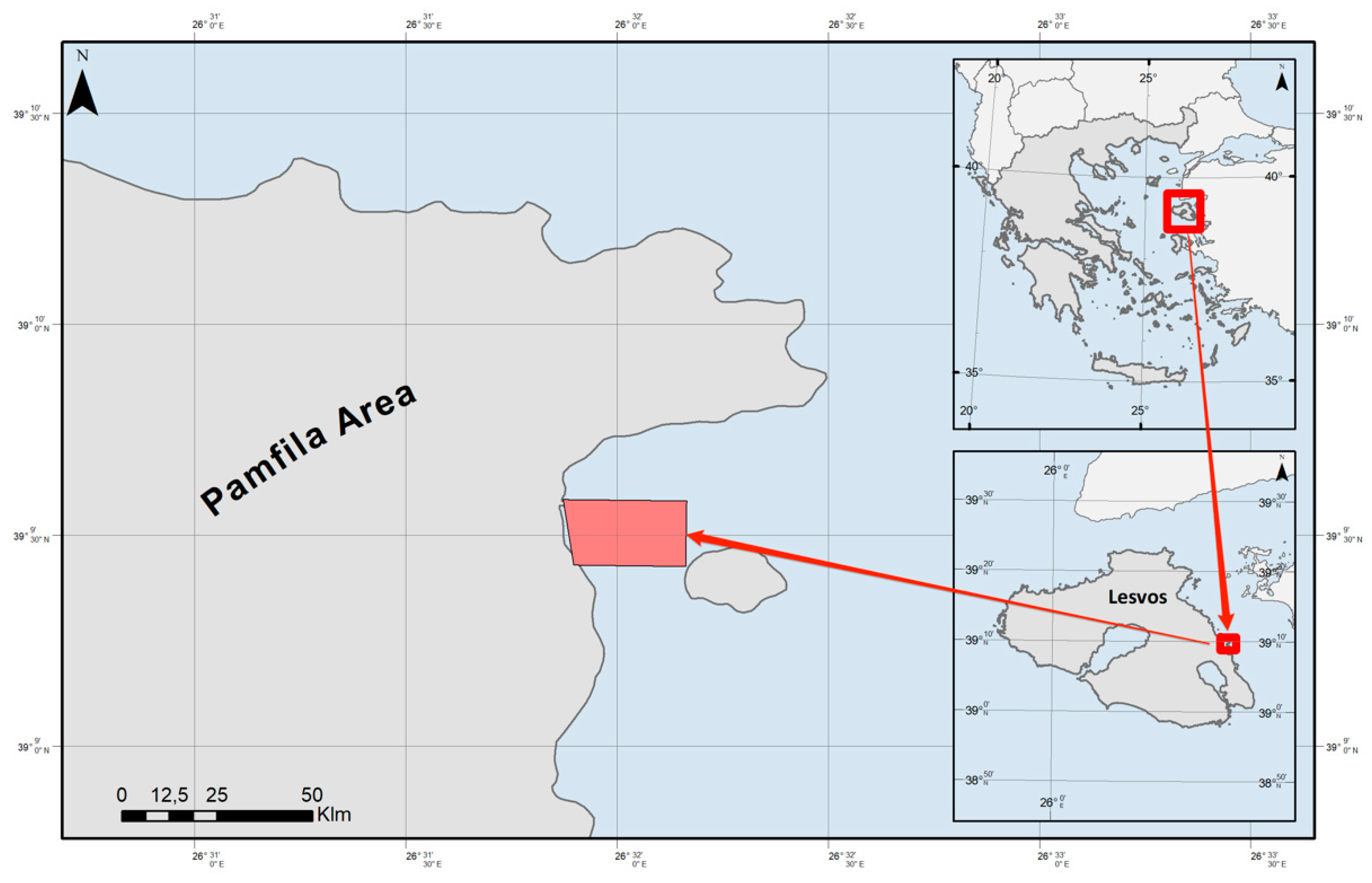
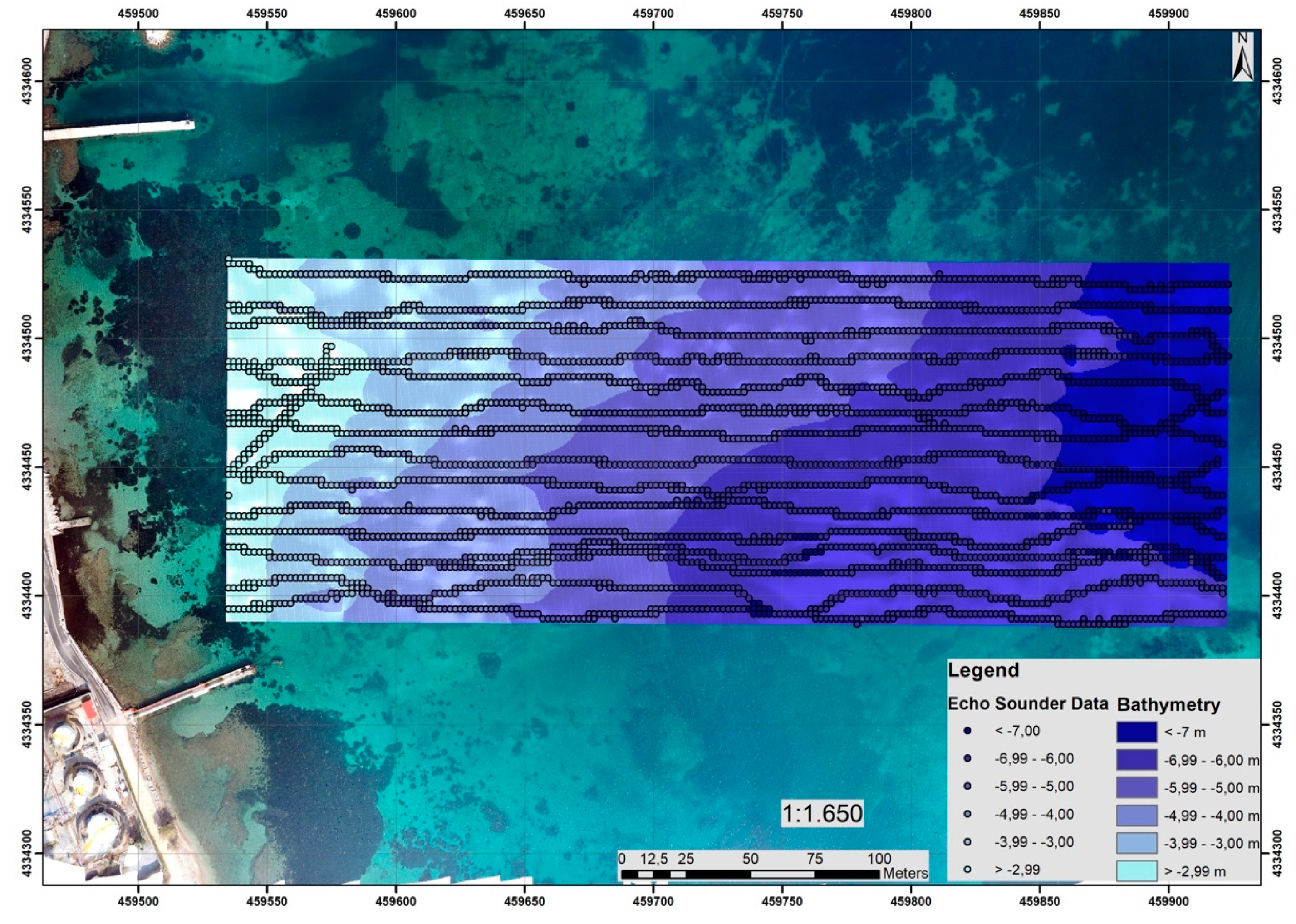
The depth in the study area was measured using a single-beam echo sounder and had a variation of 0 to 8 m. The depth zones accurately defined and proved very useful in the explanation of the results (Figure 2).

2.3. In Situ Data

In the present study, a combination of photographs taken while snorkeling and measurements derived from a single-beam echo sounder attached to a small inflatable boat were used as in situ data.

2.3.1. Divers’ Data Acquisition

The study area was initially investigated using an orthomosaic map from a previous demo flight to create sections and transects that divers would follow to capture underwater images. The selected transect orientation was designed to target all four selected classes equally. Furthermore, reference spots were selected using the abovementioned orthomosaic map to help the divers’ orientation during snorkeling. The divers’ equipment used for taking photos as in situ data was a GoPro 4 camera. The divers team followed the predetermined transects in the area and captured with an underwater image all the preselected spots having one of the four classes selected for classification. The in situ sampling took place on 06/07/2018, having a shape of a trapezium, and lasted one hour. In total, 125 underwater images were collected from the divers using a GoPro 4 Hero underwater camera. Each one of the underwater images was captured in a way to represent one training class. After quality control, 33 images were properly classified. The number of the images used for the classification was reduced by 92 due to the following reasons: (i) 18 images (14.4%) were not clearly focused on the sea bottom due to the depth; (ii) 21 images (16,8%) were not geolocated due to the repetitive sea bottom pattern (for example, sandy sea bottom); (iii) 25 images (20%) were duplicated, as they were captured in the same position by the divers to assure that the dominant class will be captured; and, finally, (iv) 28 images (23%) were blurry due to the sea state and the water quality. All images were interpreted to define the classes. Additionally, the position where these images were captured was identified by photointerpretation from the divers’ team using the tc-RGB orthomosaic.

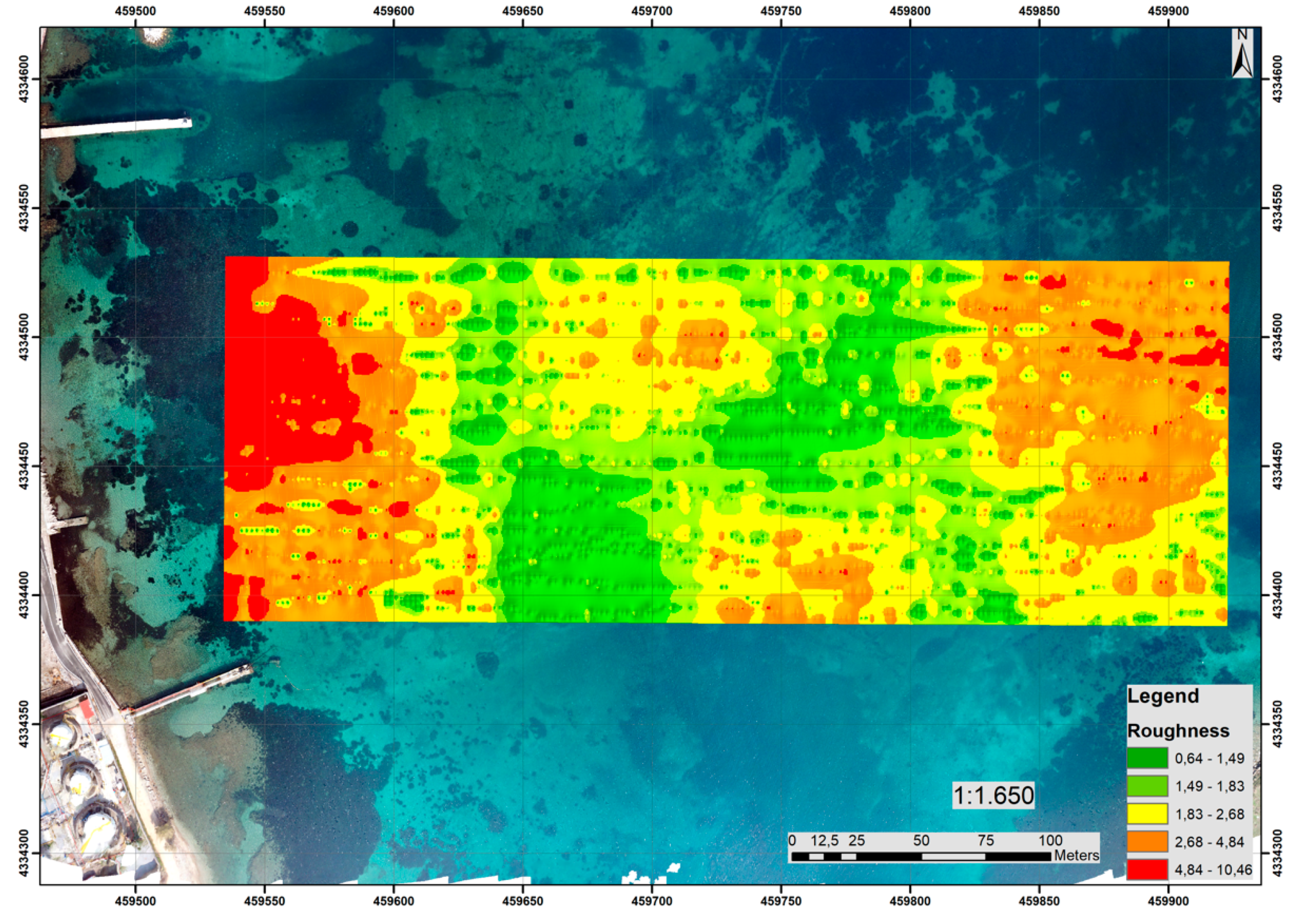
2.3.2. Echo Sounder Data Acquisition

Echo sounder data were collected by SEMANTIC TS personnel using a single-beam sound device attached to a small inflatable vessel on 06/07/2018. The measurements were based on the reflection of the acoustic pulse of the echo sounder device. SEMANTIC TS has developed a signal-processing algorithm based on discriminant analysis to scrutinize the response energy level of the sea bottom pulses [24]. The derived information includes the depth and the substrate roughness, while the precise geographical positions of the acquired data are also recorded. Roughness and bathymetry products of the study area are provided as a raster dataset (Figure 2 and Figure 3). ArcMap 10.3.1 software [25] was used to process the data, and the canvas was converted into a point vector shapefile. The point vector shapefile contained a total of 3.364 points with the roughness and bathymetry info.

2.4. UAS Data Acquisition

The UAS used for data acquisition was a vertical take-off and landing (VTOL) configuration capable of autonomous flights using preprogrammed flight paths. The configuration was a custom-made airborne system based on the S900 DJI hexacopter airframe, having a 25-min flight time with an attached payload of 1.5 Kg. The payload consisted of two sensors: a multispectral and a tc-RGB. The configuration lies in the Pixhawk autopilot system, which is an open-source UAS [26,27]. For the positioning of the UAS during the flight, a real-time kinematic (RTK) global positioning system was connected to the autopilot.

2.4.1. Air-Born Sensors Used

The true-color RGB sensor used in this study was a Sony A5100 24.3-megapixel camera with interchangeable Sigma ART 19 mm 1:2.8 DN0.2M/0.66Feet lens capable of precise autofocusing in 0.06 sec, capturing high-quality true-color RGB (tc-RGB) images. This sensor was selected because of the lightweight (0.224 kg), manual parameterization and auto-triggering capabilities, using an electronic pulse due to its autopilot. The multispectral camera was a Slantrange 3P (S3P) sensor equipped with an ambient illumination sensor for deriving spectral reflectance-based end-products, an integrated global positioning system, and an inertial measurement unit system. The S3P has a quad-core 2.26 GHz processor and an embedded 2GB RAM for onboard preprocessing. The S3P used is a modified multispectral sensor, having the wavebands adjusted to match the coastal, blue, green, and near-infrared (NIR) wavebands on the Sentinel-2 mission (

Table 1. Waveband information for the Slantrange 3P imager and Sentinel-2 missions. Coastal (C), blue (B), green (G), and near-infrared (NIR).

	Slantrange 3P		Sentinel-2A		Sentinel-2B
	Centre (nm)	Bandwidth (nm)	Centre (nm)	Bandwidth (nm)	Centre (nm)	Bandwidth (nm)
C	450	20	442.7	27	442.2	45
B	500	80	492.4	98	492.1	98
G	550	40	559.8	45	559.0	46
NIR	850	100	832.8	145	832.9	133

). The scope of the waveband modification to the S3P imager aimed at simulating Sentinel-2 data in finer geospatial resolution.

The open-access Mission Planner v1.25 software was used as a ground station for real-time monitoring of the UAS telemetry and for programming the survey missions [28].

2.4.2. Flight Parameters

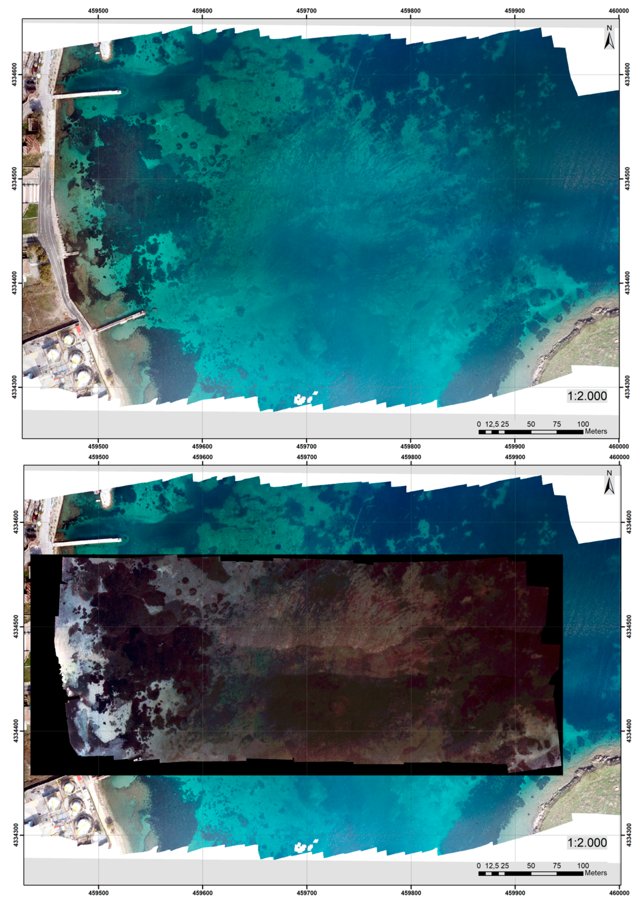
Data acquisition took place on the 8^th July 2018 in the Pamfila area. Before the data acquisition, the UAS toolbox was used to predict the optimal flight time [29]. The toolbox automates a protocol, which summarizes the parameters that affect the reliability and the quality of the data acquisition process over the marine environment using UAS. Each preprogrammed acquisition flight had the following flight parameters: 85% overlap in-track and 80% side-lap. The UAV was flying at a height of 120 m above sea level (absolute height), having a velocity of 5 m/s. Thus, the tc-RGB sensor was adjusted for capturing a photograph every 3.28 s in the nadir direction and the multispectral every 1 s. The obtained ground resolution of the tc-RGB images acquired from the UAS was 2.15 cm/pixel, and for the multispectral imager was 4.84 cm. Ground sampling resolution varied due to the focal length, pixel pitch, and sensor size of the sensors used. After a quality control inspection, the majority of the images were selected for further processing. The data acquisition information is depicted in the following table (

Table 2. The number of raw images and spatial resolution acquired using a suite of sensors attached to the unmanned aircraft system (UAS).

Name of Sensor	Number of Images	Sensor Resolution (Pixel)	Flight Height (m)	Ground Resolution (cm/Pixel)
SlantRange 3P	568	1216 × 991	120	4.84
Sony A5100	181	6000 × 4000	120	2.15

), followed by the final orthomosaics obtained from the UAV (Figure 4).

Prior to the survey missions, georeferenced targets, designed in a black and white pattern, were used as ground control points (GCP), having dimensions of 40 × 40 cm. In total, 18 targets were placed on the coastal zone of the study area. The GCP’s coordinates were measured in the Hellenic geodetic system using a real-time kinematic method yielding a total root mean square error (RMSE) of 0.244 cm.

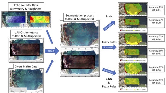
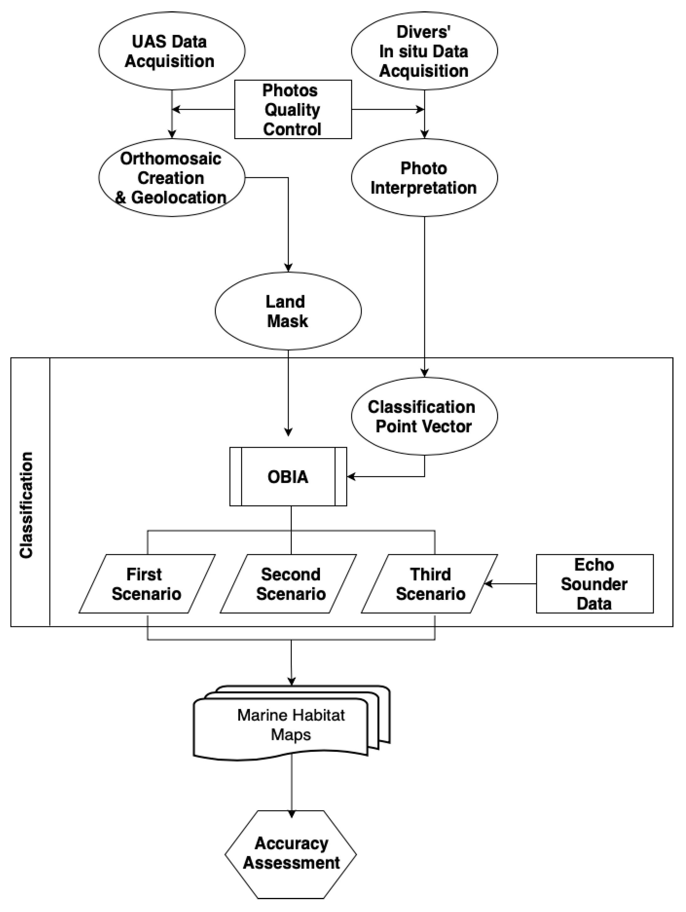
2.5. Methodological Workflow

An overview of the followed methodological workflow is given below (Figure 5). The methodology is organized into four steps: (i) data acquisition and creation of tc-RGB and multispectral orthomosaics using the UAS-SfM (structure-from-motion) framework [10,30], (ii) orthomosaics preprocessing, (iii) object-based image analysis, and (iv) accuracy assessment. After UAS and in situ data acquisition, the divers’ photos passed quality control and were interpreted to define the class that is depicted. Furthermore, in the preprocessing stage, a land mask was applied to both orthomosaics. Then, the OBIA analysis was performed, starting with the objects’ segmentation and then performing the classification of benthic substrates of the study area. The classification was implemented following three scenarios. In the first and second scenarios, the k-nearest neighbor and fuzzy rules were applied as classifiers, respectively. In the third scenario, both fuzzy rules and k-NN were applied. The in situ data collected were separated into two nonoverlapping datasets: one for training and one for accuracy assessment.

2.6. Orthomosaic Creation

Structure-from-motion (SfM) photogrammetry applied to images captured from UAS platforms is increasingly being used for a wide range of applications. SfM is a photogrammetric technique that creates two and three-dimensional visualizations from two-dimensional image sequences [31,32]. The methodology is one of the most effective methods in the computer vision field, consisting of a series of algorithms that detect common features in images and convert them into three-dimensional information. For the realization of this study, the Agisoft Photoscan 1.4.1 [33] was used, since it automates the SfM process in a user-friendly interface with a concrete workflow [32,34,35,36,37].

Georeferencing of the tc-RGB orthomosaic was achieved using 18 ground control points (GCPs). The use of GCPs for the geolocation of the tc-RGB orthomosaic had, as a result, an RMSE of 1.56 (cm). The achieved accuracy met the requirements of the authors for creating highly detailed maps. The S3P multispectral orthomosaic was georeferenced using the georeferenced tc-RGB orthomosaic as a base map [38]. An inter-comparison of the georeferenced orthomosaics was implemented to best match common characteristic reference points. Final end-products consisted of georeferenced (i) S3P—coastal (450 nm), blue (500 nm), green (550 nm), and NIR (850 nm) and (ii) Sony A5100 in true-color RGB orthomosaics. The size in pixels for the produced derivatives created from SfM is presented in the following table (

Table 3. Size in pixels of produced orthomosaics according to the used sensors: true-color RGB (Sony A5100) and multispectral (Slantrange).

Name of Sensor	Orthomosaic Size (Pixels)
SlantRange 3P	12,122 × 4103
Sony A5100	11,446 × 21,001

).

Orthomosaic Preprocessing

Before the preprocessing step, the divers’ in situ data were interpreted, and the two orthomosaics were initially checked for their geolocation accuracy. Then, the produced orthomosaics were land-masked for extracting information based solely on the pixels of the sea. The land mask was created by editing the coastline as a vector in a shapefile format using ArcMap 10.3.1 software [25].

2.7. Object-Based Image Analysis (OBIA)

For the OBIA, three necessary steps were required: (i) the segmentation procedure; (ii) the definition of the classes that will be later classified; and (iii) the delineation of the classifier, i.e., the classification algorithm defining the class where the segments will be classified.

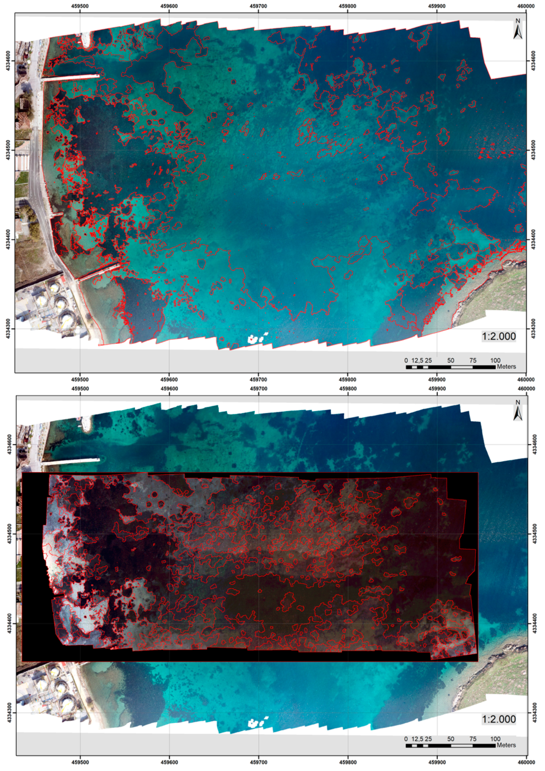
The first step of the OBIA analysis is to create objects from orthomosaics through the segmentation procedure. The orthomosaics are segmented by a multiresolution segmentation algorithm in eCognition software [39] (Figure 6). The initial outcome of the segmentation is meaningful objects defined from the scale parameters, image layer weights, and composition of the homogeneity criterion [40]. The thresholds used for these parameters were determined empirically, based on the expertise of the image interpreter. For the tc-RGB orthomosaic, the parameters of scale, shape, and compactness were set to 100, 0.1, and 0.9, respectively. For the multispectral orthomosaic, the parameters were set: 15 for the scale, 0.1 for the shape, and 0.9 for the compactness.

In the classification step, two algorithms were selected, the k-nearest neighbor (k-NN) and the fuzzy classification, using eCognition®. The k-nearest neighbor (k-NN) algorithm classifies image objects into a specific feature range and with given samples pertaining to preselected categories. Once a representative set of samples is declared, each object is classified on the resemblance of band values between the training object and the objects to be classified among the k-nearest neighbors. Thus, each segment in the image is denoted with a value equal to 1 or 0, expressing whether the object belongs to a class or not. In fuzzy classification, instead of binary decision-making, the probability of whether an object belongs to a class or not is calculated using membership functions. The limits of each class are no longer restricted using thresholds, but classification functions are used within the dataset, in which every single parameter value will have a chance of being assigned to a class [41,42]. Both classifiers are part of the eCognition® software. The k-NN algorithm was selected as a historical classification algorithm (fast deployment without the need of many samples), and fuzzy logic was selected to add specific knowledge into the classification derived from the training areas.

2.8. Classification Scenarios and Accuracy Assesment

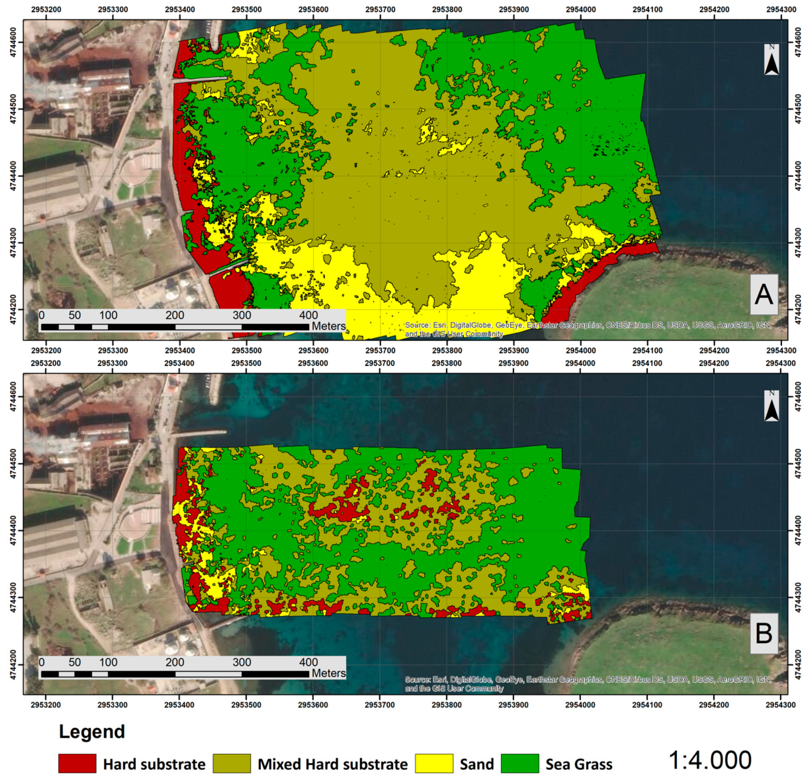
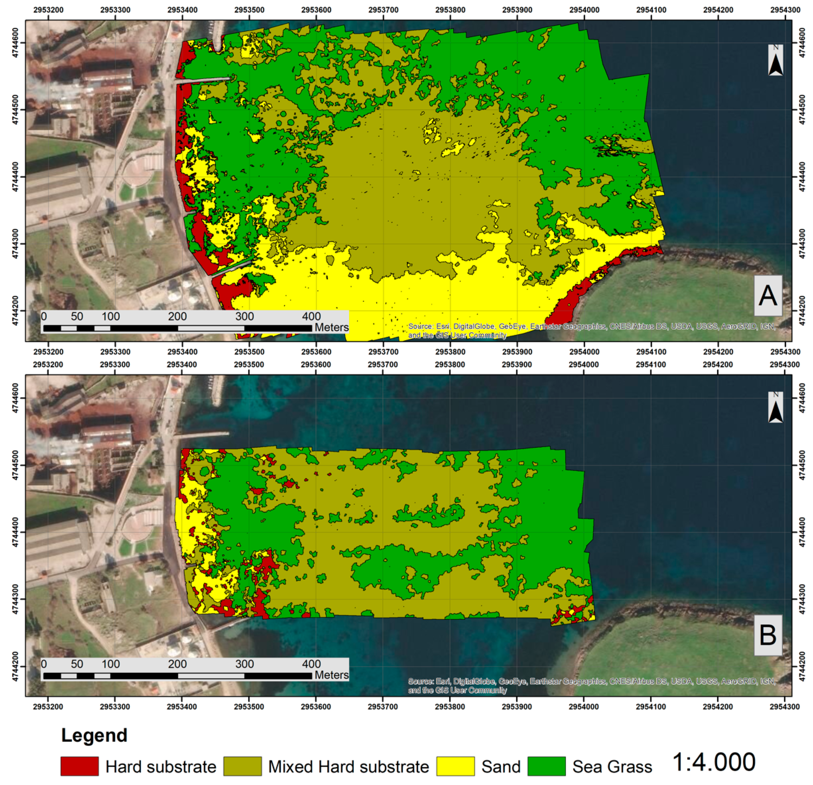
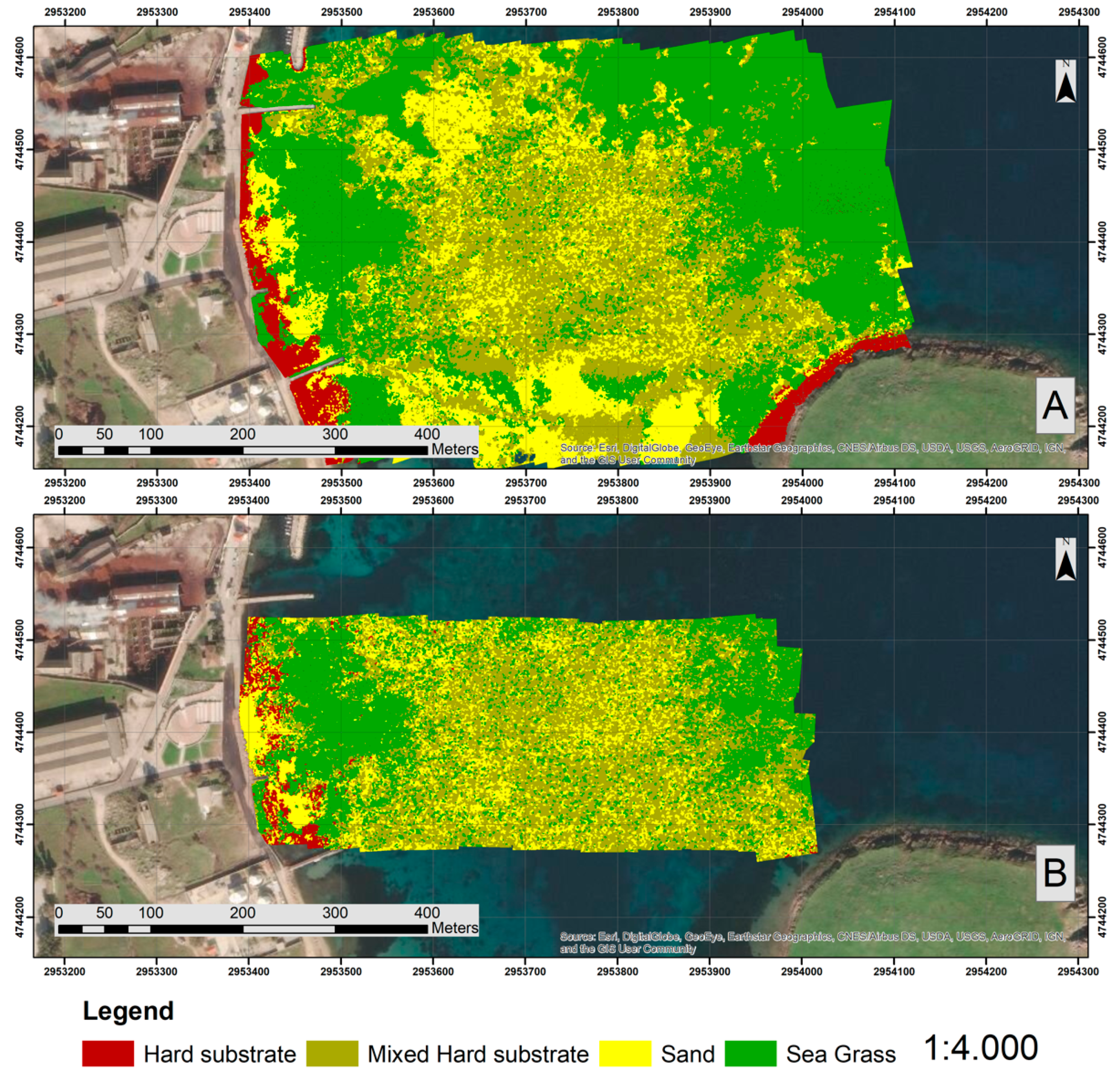
The classification step of the present study was performed in sub-decimeter UAS orthomosaics using three different scenarios for defining the best classifier for marine habitat mapping in complex coastal areas. In the first and second scenarios, the k-nearest neighbor and fuzzy rules were applied as classifiers, respectively. The third scenario was realized by applying fuzzy rules in the echo sounder data for sample creation, and the classification was performed using k-NN.

In the first scenario, in total, 60 segments were selected as training samples (15 samples per class) based on the divers’ underwater images. Each segment of the orthomosaic was classified into one of the four predefined classes using the k-NN algorithm as the classifier, and the segments of the same class were merged into one single object. The resulting classification was used for the creation of the final habitat map. This procedure was followed in both tc-RGB and multispectral orthomosaics for the first scenario.

In the second scenario, the same training sample as in the first scenario was used, and the fuzzy rules were defined and applied. The appropriate fuzzy expression for each class was created after examining the relationship between the classes for the mean segment value of the three image bands (tc-RGB). Then, the mean value of the three bands was selected as an input, and the logical rules “AND” and “OR” were used where necessary. The segments were classified using the fuzzy expressions for all classes, and the objects in the same class were merged into one single object. Thus, the results were exported as one polygon vector shapefile. As in the first scenario, the above-presented process was applied to both the tc-RGB and multispectral orthomosaics.

Finally, for the third scenario, the analysis was designed based on the following objectives: (i) examination of usefulness of the roughness echo sounder info to the classification procedure and (ii) comparison of the roughness efficiency against the underwater images photo interpretation for the creation of training samples. More specifically, a new training dataset was created based on the echo sounder’s roughness information. In total, 3028 roughness points were derived from the echo sounder dataset, and fuzzy rules were applied to 90% of the points (2724) for the creation of training samples for the classification classes. In the produced segmentation results, the k-NN algorithm was applied as the classifier for the calculation of the final classification for each of the four classes. As the small research vessel was not able to access for safety reasons to depths less than 1.5 m, we manually added samples where necessary.

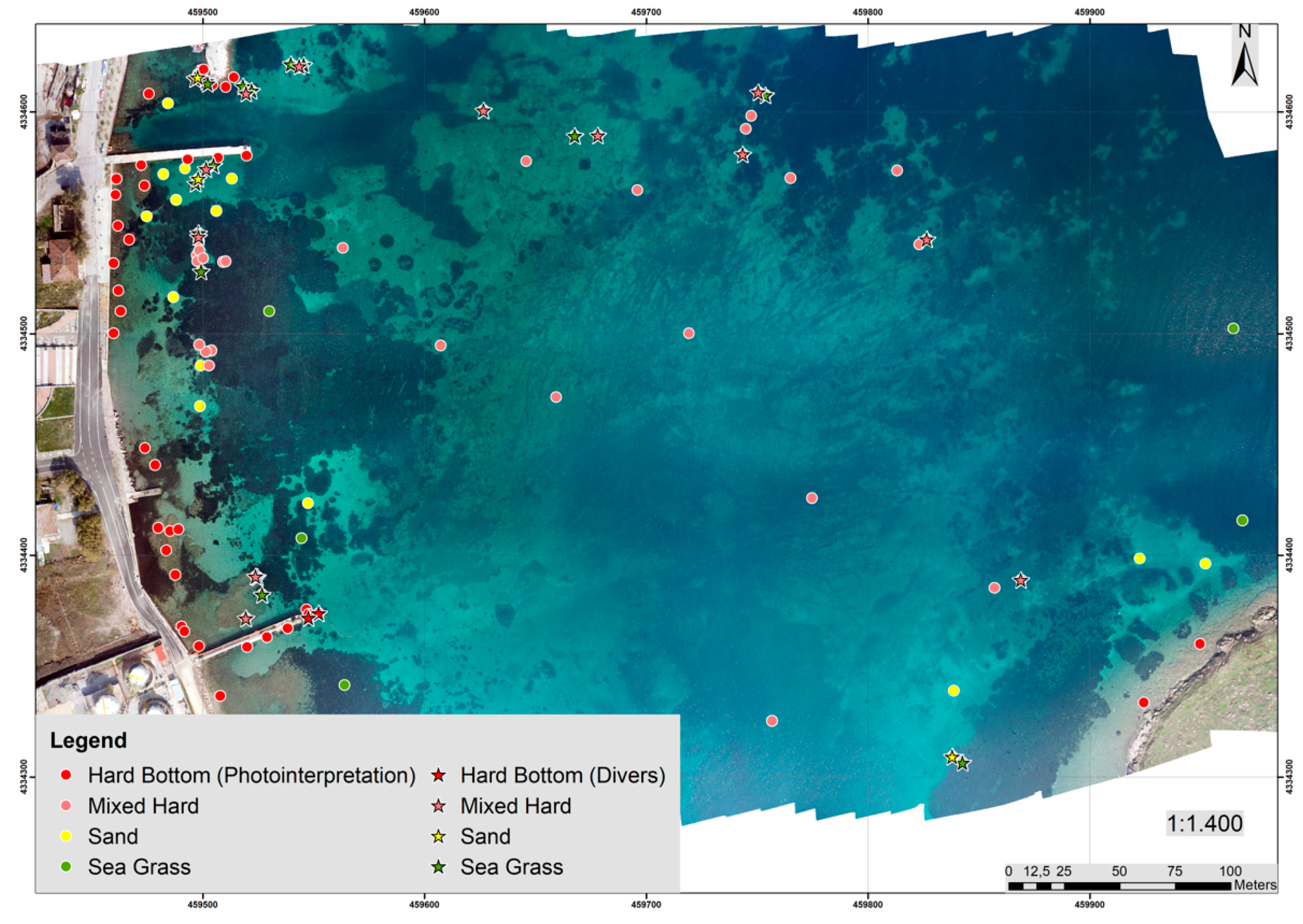
Accuracy assessment calculates the percentage of the produced map that approaches the actual field reality. In this study, we created a validation dataset that was not overlapped with the calibration dataset. In total, 120 points were generated using the geolocated underwater images (in situ divers’ data) and an expert’s photointerpretation. Initially, a point vector file was created by locating the 33 underwater images in the tc-RGM orthomosaic. Due to the small number of points produced from in situ data, the dataset was densified via photointerpretation by an expert using the high-resolution tc-RGB orthomosaic. In total, 87 points were added, and, therefore, the final point vector file ended with 120 points (30 per class). In Figure 7, all points are illustrated with colors according to their assigned taxon. In this figure, divers and photointerpretation points are depicted in round and star shapes, respectively. The 120 accuracy assessment points were firstly assigned to their relevant segments (i.e., forming 120 segments) and the total number of pixels forming the segments was used as the accuracy assessment dataset for all classifications. Furthermore, in the third scenario, 10% of the roughness points (304 points) equally distributed to all four classes were used also as accuracy assessment data. The accuracy matrices created for all scenarios provided information regarding the user and producer accuracy, overall accuracy, and the Kappa index coefficient (

Table 4. Accuracy matrix for the true-color RGB (tc-RGB) orthomosaic, with k-nearest neighbor as the classifier. KIA: Kappa index of agreement.

		Reference Data
		Sea Grass (Pixels)	Mixed Hard Substrate (Pixels)	Sand (Pixels)	Hard Bottom Substrate (Pixels)	Sum (Pixels)
Training Data	Sea Grass	37,2384	0	0	4053	37,6437
	Mixed Hard Substrate	18,174	52,3604	164,822	32,669	739,269
	Sand	25,776	85,351	172,498	4167	287,792
	Hard Bottom Substrate	6642	52,941	0	433,426	493,009
	Sum	422,976	661,896	337,320	474,315
	Producers’ accuracy	0.88	0.79	0.51	0.91
	Users’ accuracy	0.98	0.70	0.60	0.88
	KIA per class	0.85	0.66	0.42	0.88
		Total accuracy		0.79
		KIA		0.71

,

Table 5. Accuracy matrix for the multispectral orthomosaic with k-nearest neighbor as the classifier.

		Reference Data
		Sea Grass (Pixels)	Mixed Hard Substrate (Pixels)	Sand (Pixels)	Hard Bottom Substrate (Pixels)	Sum (Pixels)
Training Data	Seagrass	13,677	9800	0	2333	25,810
	Mixed Hard Substrate	0	19,428	0	2038	21,466
	Sand	0	0	14,585	1294	15,879
	Hard Bottom Substrate	0	3752	1311	22,312	27,375
	Sum	13,677	32,980	15,896	27,977
	Producers accuracy	1	0.59	0.92	0.8
	Users accuracy	0.53	0.91	0.92	0.82
	KIA per class	1	0.46	0.9	0.71
		Total accuracy		0.77
		KIA		0.7

,

Table 6. Accuracy matrix for the tc-RGB orthomosaic applying the fuzzy rules.

		Reference Data
	Classes	Sea Grass (Pixels)	Mixed Hard Substrate (Pixels)	Sand (Pixels)	Hard Bottom Substrate (Pixels)	Sum (Pixels)
Training Data	Sea Grass	320,025	75,491	21,987	10,838	428,341
	Mixed Hard Substrate	1807	404,691	43,224	4062	453,784
	Sand	101,144	135,194	272,109	73,351	581,798
	Hard Bottom Substrate	0	46,520	0	386,064	432,584
	Sum	422,976	661,896	337,320	474,315
	Producers accuracy	0.76	0.61	0.81	0.81
	Users accuracy	0.75	0.89	0.47	0.89
	KIA per class	0.69	0.49	0.72	0.76
		Total accuracy		0.73
		KIA		0.64

,

Table 7. Accuracy matrix for the multispectral orthomosaic applying the fuzzy rules.

		Reference Data
	Classes	Sea Grass (Pixels)	Mixed Hard Substrate (Pixels)	Sand (Pixels)	Hard Bottom Substrate (Pixels)	Sum (Pixels)
Training Data	Sea Grass	13,677	5761	3333	0	22,771
	Mixed Hard Substrate	0	19,998	0	4371	24,369
	Sand	0	2786	12,563	16,633	31,982
	Hard Bottom Substrate	0	4435	0	6973	11,408
	Sum	13,677	32,980	15,896	27,977
	Producers accuracy	1	0.6	0.79	0.25
	Users accuracy	0.6	0.82	0.39	0.61
	KIA per class	1	0.46	0.68	0.14
		Total accuracy		0.59
		KIA		0.46

,

Table 8. The tc-RGB data classification accuracy matrix for the multispectral orthomosaic.

		Reference Data
	Classes	Sea Grass (Pixels)	Mixed Hard Substrate (Pixels)	Sand (Pixels)	Hard Bottom Substrate (Pixels)	Sum (Pixels)
Training Data	Sea Grass	379,034	84,089	14,876	28,568	506,567
	Mixed Hard Substrate	40,103	276,346	108,280	8800	433,529
	Sand	3442	259,310	214,157	36,108	513,017
	Hard Bottom Substrate	394	42,069	7	400,810	443,280
	Unclassified	3	82	0	29	114
	Sum	422,976	661,896	337,320	474,315
	Producers accuracy	0.9	0.42	0.63	0.85
	Users accuracy	0.75	0.64	0.42	0.9
	KIA per class	0.86	0.24	0.5	0.8
		Total accuracy		0.67
		KIA		0.56

, and

Table 9. Echo sounder data classification accuracy matrix for the multispectral orthomosaic.

		Reference Data
	Classes	Sea Grass (Pixels)	Mixed Hard Substrate (Pixels)	Sand (Pixels)	Hard Bottom Substrate (Pixels)	Sum (Pixels)
Training Data	Sea Grass	11,858	7811	4530	1987	26,186
	Mixed Hard Substrate	1681	13,615	2156	2936	20,388
	Sand	133	7042	4747	6685	18,607
	Hard Bottom Substrate	2	4504	4457	16,357	25,320
	Unclassified	3	8	6	12	29
	Sum	13,677	32,980	15,896	27,977
	Producers accuracy	0.87	0.41	0.3	0.58
	Users accuracy	0.45	0.67	0.26	0.65
	KIA per class	0.81	0.24	0.12	0.42
		Total accuracy		0.51
		KIA		0.35

).

3. Results

In this section, the classification results of the three scenarios are presented for both the tc-RGB and multispectral data. The classification was performed using four habitat classes: (i) hard substrate, (ii) seagrass, (iii) sand, and (iv) mixed hard substrate.

3.1. Scenario 1: k-Nearest Neighbor as Classifier

In the first scenario, k-nearest neighbor (k-NN) was used as the classifier and, when it was applied to the tc-RGB orthomosaic, it resulted in the classification map depicted in Figure 8A. According to the bathymetry, the hard substrate appears in the intertidal and the very shallow zone at depths of 0 to 1.5 m. The sand class covers mainly the southern part of the study area, and the mixed hard substrate is located mainly in the middle of the study area, at depths of 2.5 to 6.5 m. The seagrass (Posidonia Oceanica) class is divided into two parts: one on the west side of the beach (right next to the hard substrate) at a depth of about 1.5 to 3.5 m and one on the eastern part of the beach where the depths vary approximately 6.5 to 7.9 m. The percentage of the segments that belong to each of the classes is 28.9%, 11.5%, 34.9%, and 24.8% for hard substrate, sand, mixed hard substrate, and seagrass, respectively. Additionally, the percent areal coverages in square meters for each class were calculated for this scenario. The area covered from the tc-RGB is 178,386 square meters, and the sand class is presented as occupying 16.29% of the total area mapped. The other classes’ percentage areal coverage are 33.04% for seagrass, 44.50% for mixed hard substrate, and 6.17% for the hard bottom.

The overall accuracy of the classification was 79%, and the Kappa index of agreement (KIA) was 0.71 (Table 4). The sand class presented a lower accuracy compared to the other classes. Several objects in this class have been incorrectly classified as mixed hard substrate.

The classification results of the multispectral orthomosaic are illustrated in Figure 8B. It can be noted that the hard substrate appears mainly in the intertidal and the shallow zone at depths of 0 to 3.5 m, having been assigned 31.9% of the total objects. The sand class covers small areas of the western part of the study area, and the mixed hard substrate is located mainly in the middle of the study area, at depths of about 2.5 to 9.9 m. The seagrass is scattered almost throughout the study area, covering a wide depth range of about 0 to 9.9 m. The classified object percentages for the sand, mixed hard substrate, and seagrass classes are 20.8%, 27.8%, and 19.5%, respectively. In an area of 90,857 square meters covered by multispectral orthomosaic, the percent areal coverages by class are 3.78%, 51.55%, 36.54%, and 8.13% for sand, sea grass, mixed hard substrate, and hard substrate, respectively.

The achieved overall classification accuracy was 77%, and the KIA coefficient was equal to 0.70 (Table 5). In this case, the mixed hard substrate class presented lower accuracy in comparison with the rest of the classes, since several objects have been incorrectly classified as seagrass and mixed hard substrate.

3.2. Scenario 2: Fuzzy Rules as Classifier

In the second scenario, fuzzy rules were used as the classifier, and the four classes created from the tc-RGB and multispectral orthomosaics are illustrated in Figure 9A,B, respectively. According to the classification results for the tc-RGB orthomosaic, the percentage of the assigned objects for the hard substrate, sand, mixed hard substrate, and seagrass classes are 27.9%, 20%, 29.9%, and 23.1%, respectively. For this scenario, the percentage areal coverage was calculated to be 23.35% sand, 35.35% seagrass, 37.27% mixed hard substrate, and 4.02% hard substrate.

When fuzzy rules were used as the classifier, the overall accuracy was 73%, and the coefficient KIA was 0.64 (Table 6). In this scenario, the mixed hard substrate class presented lower accuracy in comparison with the other three classes, since several objects of this class have been incorrectly classified as hard substrate, sand, and seagrass.

From the classification results of the multispectral orthomosaic (Figure 9B), the seagrass class comes into sight, divided into two parts. The first part is on the west side of the beach (right next to the sand class) at depths of about 1.5 to 3.5 m and the second on the eastern part of the beach. In this part, the depths vary approximately from 6.5 to 7.9 m. The percentage of each class object is 13.1%, 23.6%, 37.6%, and 25.7% for hard substrate, sand, mixed hard substrate, and seagrass, respectively. Furthermore, the percentage of areal calculations saw that the sand class covers 4.99%, while the seagrass, mixed hard substrate, and hard bottom are covering 40.25%, 51.50%, and 3.27% of the total classified area, respectively. The overall classification accuracy obtained by the fuzzy rules is 59%, and the coefficient K is equal to 0.46 (Table 7). In this classification scenario, the hard substrate and mixed hard substrate classes present lower accuracy, since several objects in these classes have been incorrectly classified.

3.3. Scenario 3: k-NN and Fuzzy Rules as Classifiers

In the scenario where a combination of the fuzzy rules and k-NN are used as the classifiers, the four classes created from the classification of the tc-RGB orthomosaic are represented in Figure 10A. The percentage of the assigned objects for the four classes is 31.6%, 16.9%, 21.6%, and 29.8% for hard substrate, sand, mixed hard substrate, and seagrass, respectively. The classes created from the tc-RGB orthomosaic present the following results in percent areal coverage. The class sand has 21.66%. The overall classification accuracy is 67%, and the KIA coefficient is equal to 0.56 (Table 8). The mixed hard substrate and sand classes presented lower accuracy compared to the rest of the classes, regarding the tc-RGB orthomosaic in this scenario. Several objects of the mixed hard substrate and sand classes were incorrectly classified into other classes.

The multispectral orthomosaic classification results derived from scenario 3 are illustrated in Figure 10B. For each class, the percentage of the assigned objects was 35.1%, 10.2%, 29.3%, and 25.5% for hard substrate, sand, mixed hard substrate, and seagrass, respectively. The areal percentage coverage calculation results for the multispectral orthomosaic in scenario 3 were 21.72% coverage for sand, 33.62% for seagrass, 42.94% for mixed hard substrate, and, finally, 2.72% for hard substrate. In this scenario, the overall classification accuracy was relatively low (51%), and the coefficient KIA was very low (0.35) (Table 9). The hard substrate, mixed hard substrate, and sand classes presented lower accuracy compared to the seagrass class using the k-NN and fuzzy rules as classifiers. Several objects in the above-mentioned classes have been incorrectly classified.

The third scenario presents scattered areas of mixed hard substrate, in contrast to scenarios 1 and 2. The main difference is located in the center of the scene where the mixed classes are. On the contrary, all scenarios depict nicely the seagrass class in both shallow and deep waters. Hard bottom is well-defined in all scenarios. The multispectral dataset seems not to classify correctly the mix hard substrate and the sand classes.

Table 10. Brief table of total accuracies for the tc-RGB and multispectral orthomosaics of the three scenarios of the study.

Scenario No.	Classifier	Training Data	Orthomosaic	Total Accuracy	Kappa Index
Scenario 1	k-Nearest Neighbor	Underwater images	tc-RGB	79%	0.71
		Underwater images	Multispectral	77%	0.7
Scenario 2	Fuzzy Rules	Underwater images	tc-RGB	73%	0.64
		Underwater images	Multispectral	59%	0.46
Scenario 3	k-Nearest Neighbor & Fuzzy Rules	Echo Sounder roughness	tc-RGB	67%	0.56
			Multispectral	51%	0.35

summarizes the overall accuracy of the three scenarios. In all scenarios, the tc-RGB orthomosaic responded better than the multispectral orthomosaic. The best performance (79%) was given in the first scenario for the k-NN classifier applied to the tc-RGB orthomosaic. The use of echo sounder data as training data did not increase the quality of the final classification maps, as the authors expected. On the contrary, the accuracy was worse when echo sounder data were used as training data, compared to those where solely underwater images were applied.

4. Discussion and Conclusions

In this work, we have shown that the utilization of UAS high in resolution and accuracy aerial photographs, in conjunction with the OBIA, can create quality habitat mapping. We demonstrated that habitat mapping information could be automatically extracted from sub-decimeter spatial true-color RGB images acquired from UAS. High-resolution classification maps produced from UAS orthomosaic using the OBIA approach enables the identification and measurement of habitat classifications (sand, hard bottom, seagrass, and mixed hard substrate) in the coastal zone over the total extent of the mapped area. The detailed geoinformation produced provides scientists with valuable information regarding the current state of the habitat species, i.e., the environmental state of sensitive coastal areas. Moreover, the derived data products enable in-depth analysis and, therefore, the identification of change detections caused by anthropogenic interventions and other factors.

The purpose of this paper was twofold: (a) to compare two types of orthomosaics, the tc-RGB and the multispectral, captured over a coastal area using OBIA with different classifiers to map the selected classes and (b) to examine the usefulness of the bathymetry and the roughness information derived from the echo sounder as training data to the UAS-OBIA methodology for marine habitat mapping.

From the comparison of the classification results, it can be concluded that the tc-RGB orthomosaic produces more valuable and robust results than the multispectral one. This is caused due to the multispectral imager specifications. More specifically, the multispectral sensor receives data from four discrete bands, and a global shutter is used. As a result, the sensor captures photos in a shorter time compared to the tc-RGB camera. Thus, the exposure time is shorter in the multispectral (SlantRange modified imager) than in the true-color RGB (Sony A5100) sensor, causing less light energy. In addition, during the process of the multispectral orthomosaic creation due to the data quality of the initial images, the final derivative was not uniform, thus presenting discrete irregularities. These anomalies appeared due to different illumination conditions and the sun glint; therefore, the multispectral orthomosaic classification presents lower accuracy values. It is crucial to follow a specific UAS flight protocol before each data acquisition, as presented by Doukari et al. in [29,43], for eliminating these anomalies. It should be mentioned that the UAS data acquisition procedure works fine over land, presenting a high accuracy level. However, it is not performed adequately over moving water bodies, especially when having a large extent; thus, no land is presented in the data.

Three scenarios were examined for the classification of the marine habitats using different classifiers. The k-nearest neighbor and fuzzy rules were applied in the first and second scenarios, respectively, and a combination of the fuzzy rules and k-NN algorithm in the third scenario. From the evaluation of the three scenarios’ classification results, it can be concluded that the use of the tc-RGB instead of the multispectral data provides better accuracy in detecting and classifying marine habitats by applying the k-NN as the classifier. The overall accuracy using the K-NN classifier was 79%, and the Kappa index (KIA) was equal to 0.71. The results illustrate the effectiveness of the proposed approach when applied to sub-decimeter resolution UAS data for marine habitat mapping in complex coastal areas.

Furthermore, this study demonstrated that the roughness information derived from the echo sounder did not increase the final classification accuracy. Although the echo sounder roughness can be used to discriminate classes and produce maps of the substrates, it cannot be used directly as training data for classifying UAS aerial data. Based on the echo sounder signal, a proper roughness analysis should be initially performed to produce habitat maps, which in later stages could be used as training and validation data for the UAS data.

The results showed that UAS data revealed the sub-bottom complexity to a large extent in relatively shallow areas, providing accurate information and high spatial resolution, which permits habitat mapping with extreme detail. The produced habitat vectors are ideal as reference data for studies with satellite data of lower spatial resolution. Since UAS sub-decimeter spatial resolution imagery will be increasingly available in the future, it could play an important role in habitat mapping, as it serves the needs of various studies in the coastal environment. Finally, the combination of OBIA classification with UAS sub-decimeter orthomosaics implements a very accurate methodology for ecological applications. This approach is capable of recording the high spatiotemporal variability needed for habitat mapping, which has turned into a prime necessity for environmental planning and management.

UAS are increasingly used in habitat mapping [7,12,16,17,18,44], since they provide high-resolution data to inaccessible areas at a low cost and with high temporal repeatability [10,45,46]. The use of a multispectral camera with similar wavelengths to the Sentinel-2 satellite wavelengths was examined for the first time in the present study. Results indicated that the tc-RGB and multispectral orthomosaic perform similarly, and there is no significant advantage of the multispectral camera. This can be explained twofold: (a) due to the fact that the multispectral camera is designed for land measurements and due to the inherited optical properties that cannot distinguish small radiometric differences in water, and (b) the multispectral orthomosaic was problematic due to the large differences in actual multispectral images as a result of large overlaps between them. The multispectral imager over sea areas should contain small overlaps and should gain data in short shutter speeds, i.e., with larger acquisition times. Additionally, results show that echo sounder roughness should not be used for training classification algorithms. The total accuracy of the third scenario in both orthomosaics clearly indicates the inadequacy of bottom roughness for training datasets.

Moving forward, the authors believe that the rapidly developing field of lightweight drones and the miniaturization and the rapid advance of true-color RGB, multispectral, and hyperspectral sensors for close remote sensing will soon allow a more detailed mapping of marine habitats based on spectral signatures.