Evapotranspiration in the Tono Reservoir Catchment in Upper East Region of Ghana Estimated by a Novel TSEB Approach from ASTER Imagery


1
State Key Laboratory of Biogeology and Environmental Geology, China University of Geosciences, Wuhan 430078, China
2
School of Environmental Studies, China University of Geosciences, Wuhan 430078, China
*
Author to whom correspondence should be addressed.
Remote Sens. 2020, 12(3), 569; https://0-doi-org.brum.beds.ac.uk/10.3390/rs12030569
Submission received: 3 January 2020
/
Revised: 6 February 2020
/
Accepted: 6 February 2020
/
Published: 8 February 2020
(This article belongs to the Section Biogeosciences Remote Sensing)
Abstract
:Evapotranspiration (ET) is dynamic and influences water resource distribution. Sustainable management of water resources requires accurate estimations of the individual components that result in evapotranspiration, including the daily net radiation (DNR). Daily ET is more useful than the evaporative fraction (EF) provided by remote sensing ET models, and to account for daily variations, EF is usually combined with the DNR. DNR exhibits diurnal and spatiotemporal variations due to landscape heterogeneity. In the modified Two-Source Energy Balance (TSEB) approach by Zhuang and Wu, 2015, ecophysiological constraint functions of temperature and moisture of plants based on atmospheric moisture and vegetation indices were introduced, but the DNR was not spatially accounted for in the estimation of the daily ET. This research adopted a novel approach that accounts for spatiotemporal variations in estimated daily ET by incorporating the Bisht and Bras DNR model in the modified version of the TSEB model. Advanced Spaceborne Thermal Emission and Reflection Radiometer (ASTER) satellite imagery over the Tono irrigation watershed within the Upper East Region of Ghana and Southern Burkina Faso were used. We estimated the energy fluxes of latent and sensible heat as well as the net radiation and soil heat fluxes from the satellite images and compared our results with ground-based measurements from an eddy covariance (EC) station established by the West African Science Service Center on Climate Change and Adapted Land Use (WASCAL) within the watershed area. We noticed a similarity between our model estimated fluxes and ET with the ground-based EC station measurements. Eight different land use/cover types were identified in the study area, and each of these contributed significantly to the overall ET variations between the two study periods: December 2009 and December 2017. For instance, due to a higher leaf area index (LAI) for all vegetation types in December 2009 than in December 2017, the ET for December 2017 was higher than that for December 2009. We also noticed that the land use/cover types within the footprint area of the EC station were only six out of the eight. Generally, all the surface energy fluxes increased from December 2009 to December 2017. Mean ET varied from 3.576 to 4.486 (mm/d) for December 2009 while from 4.502 to 5.280 (mm/d) for December 2017 across the different land use/cover classes. Knowledge of the dynamics of evapotranspiration and adoption of cost-effective methods to estimate its individual components in an effective and efficient way is critical to water resources management. Our findings provide a tool for all water stakeholders within watersheds to manage water resources in an engaging and cost-effective way.

1. Introduction
Surface evapotranspiration (ET) or latent heat flux plays a pivotal role in the energy, water as well as carbon cycles, and is common to all three. It provides the link between energy and water budgets at the land surface; between terrestrial water as well as carbon cycle by way of transpiration of vegetation, plays a significant role in coupling the ocean and land surfaces to the atmosphere, and operates over daily and seasonal time scales. It plays a significant role in water yield predictions, drought analysis, designing of irrigation and water supply projects, management of water quantity and quality, and environmental concerns. On account of these, practical theories of ET and their influence on catchment hydrology are still elusive [1,2,3].
Since direct measurements of vapor flux in the atmosphere is difficult, [4,5] most of the methods only monitor the system changes. ET can be estimated by direct methods (e.g., using lysimeters), micrometeorological methods (e.g., energy balance), and hydrological methods (e.g., water balance). These methods mostly give point-based estimations of ET with the deficiency of not being able to represent ET assessments at large scales [6,7]. Remote sensing alternatives provide substantial inputs at varying spatiotemporal resolutions to overcome the challenges associated with the point-based estimation methods. Remotely sensed data cover large areas while ensuring consistency in quality and frequency of revisit time of the same location to provide updates [8,9,10,11]. Remote sensing offers several parameters necessary for surface energy balance (SEB) models, such as the land surface temperature, surface albedo, and vegetation index to compute ET for individual pixels to the entire raster image.
Several satellite sensors provide remotely sensed data at varying spatiotemporal resolutions such as the Landsat 8 with 30 m spatial resolution for its red and near-infrared bands and 100 m spatial resolution for its thermal infrared bands. ASTER, on the other hand, offers satellite imagery at 15 m spatial resolution for its visible near-infrared bands and 90 m spatial resolutions for its thermal infrared bands. ASTER data was therefore used in our analysis owing to better spatial resolution. ASTER satellite imagery has provided several parameters for SEB models for the retrieval of reliable estimates for ET at both local and regional scales [12,13,14,15,16]. Land use and land cover derived from satellite imagery provide tools for predicting the spatial variation of vegetation and the effect of land use practices that control ET and soil moisture [17,18,19].
Surface Energy Balance (SEB) algorithms have been developed for the estimation of evapotranspiration. These SEB algorithms may be categorized into either one-source (1S) or dual-source (2S) depending on whether the energy budget due to the soil and vegetation are analyzed separately or by combining them. The soil and vegetation are assumed to be a “big leaf” with uniform aerodynamic resistance and temperature for the transfer of heat at equal height for the 1S models, thereby allowing for a combined analysis of the energy budget. The 1S-SEB models include: Operational Simplified Surface Energy Balance (SSEBop) [20,21]; Mapping Evapotranspiration at High Resolution with Internalized Calibration (METRIC) [22]; Surface Energy Balance System (SEBS) [23]; Simplified Surface Energy Balance Index (S-SEBI) [24]; and Surface Energy Balance Algorithm for Land (SEBAL) [25]. Studies indicate that one-source models perform poorly in sparsely vegetated areas, while they give satisfactory results in areas of dense canopy cover [26,27]. The 2S alternative treats the soil and vegetation as different sources or sinks for heat fluxes, resulting in separate analysis of their energy budget. The 2S-SEB models include Enhanced Two-Source Evapotranspiration Model for Land (ETEML) [28]; Dual Temperature Difference (DTD) [29]; Atmosphere–Land Exchange Inverse (ALEXI) [30]; Two-Source Time Integrated Model (TSTIM) [31]; and Two-Source Energy Balance (TSEB) model [32]. The 2S approach to modeling of energy fluxes is appropriate for areas that are partially covered by vegetation since such areas experience a net flux characterized by plant and soil in addition to the signals sensed remotely.
The TSEB model operates the ET partitioning by using the land surface temperature (LST), fractional vegetation cover (fc), and the Priestley–Taylor (PT) assumption that relates transpiration to net radiation via a fixed PT coefficient (). The patch and layer approach is used to describe the TSEB model. The patch model considers each patch separately with the total flux of the individual pieces calculated from the average of the different fluxes (canopy and soil) and weighted according to their area in relative terms (fractional vegetation cover, fc) [33]. The layered approach, on the other hand, uses two sources (a substrate and an upper canopy) that are different to represent vegetation that exchanges latent and sensible heat with the atmosphere [32]. Fluxes from each layer are then summed up as the total flux for the entire canopy [33].
The required inputs while adopting the TSEB patch and layer approaches are the canopy and soil temperatures. The temperature can be obtained by measurement of radiometric temperatures at two view angles. However, it is not possible to get the measure of radiometric temperature (Trad) at two view angles from satellites (e.g., ASTER, Landsat 8, FY3A, HJ-1B, and MODIS) because they are only available at single-view angles. Researchers adopted several approaches to overcome these challenges, including the use of data observed from the field to test the component temperatures for TSEB patch modeling, the adoption of thermal remote sensing inputs for the light use efficiency model of the TSEB scheme, the use of a sketch from fc-Trad feature space of a trapezoid to derive the temperature components from the TIME patch model, and finally, the use of the iterative approach of Priestley–Taylor to derive the component temperatures [34,35,36,37,38]. The iterative approach of Priestley–Taylor avoids the estimation of vapor pressure deficit and provides for the derivation of the component temperatures by using an estimated value of the canopy ET at the initial stage. It then builds on the derived temperatures based on this initial canopy ET to provide realistic values used for deriving the sensible and latent heat fluxes.
The derived components of the TSEB model include latent and sensible heat fluxes. At regional applications of the TSEB model, uncertainties are introduced in the derivation of these components. This is a result of adopting the iterative approach of the Priestley–Taylor scheme in the TSEB model. The Priestley–Taylor iterative approach overestimates the canopy ET. ET by the energy balance approach includes components from the latent and sensible heat fluxes. The iterative approach of the Priestley–Taylor underestimates the total sensible heat flux and overestimates the total latent heat flux. This results in lower soil wetness, high air drying power, and sparse vegetation cover [36,37,39,40]. The iteration approach proposed by [32] in the Priestley–Taylor formulation does not make provision for a reasonable reduction to the initial canopy ET. This deficiency prompted a modification of the original TSEB model to offset the uncertainties and thereby provide canopy latent heat fluxes accurate enough for solving the model [15]. In the modification, ecophysiological constraint functions of temperature and moisture of plants based on atmospheric moisture and vegetation indices were introduced by using formulations from the Priestley–Taylor Jet Propulsion Laboratory (PT-JPL) algorithm [15,41]. The modified TSEB model [15] was later validated for the temperate/humid continental climatic regions in China [42,43].
However, in their approach to estimating the daily evapotranspiration (ET24, mm), [15] used the point value of the daily net radiation (Rn,24). The radiation components are variedly influenced by the surface heterogeneity and by the presence, type, and diurnal distribution of clouds. As a result, the net surface radiation varies spatially as well as temporally. Daily net radiation essentially follows the shape of the diurnal variation of the land surface temperature during day-time. As these measurements are strongly influenced by surface heterogeneity, it is difficult either to extend measurements made at a specific location to other sites [44] or to extrapolate them to regional scales.
This paper explores the usefulness of the modified TSEB model [15] for surface flux estimation across different land use types for two study periods in the tropical savanna climatic region [43,45] of the Tono Catchment within Ghana and Burkina Faso using satellite ASTER imagery by adopting a novel approach of estimating the daily net radiation from satellite imagery using the daily net radiation method proposed by [46]. The estimations from satellites were validated using measurements from the eddy covariance system from one station over the catchment area established by the West African Science Service Center on Climate Change and Adapted Land Use (WASCAL).
2. Materials and Methods
2.1. Site of Study, Data, and Instrumentation
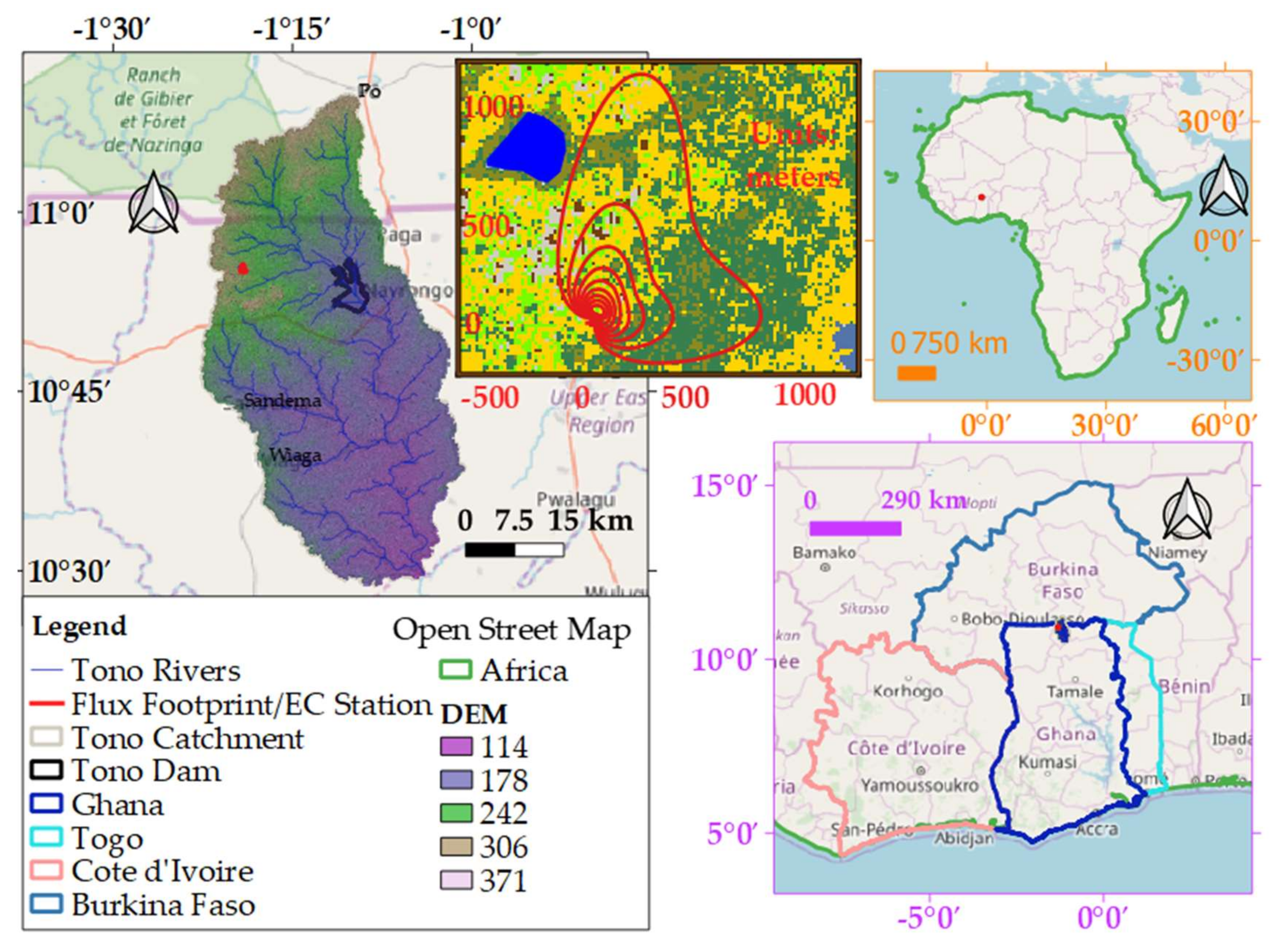
The watershed of the study area (Tono catchment) is about 1873 sq. km and spans two countries; Ghana and Burkina Faso within the Western part of Africa (Figure 1). About 85% of the watershed area is in Ghana. Ghana is bordered to the East by Togo, to the West by Cote d’Ivoire (the land of ivory), to the North by Burkina Faso, and to the South by the Gulf of Guinea and the Atlantic Ocean. Topography of the Tono catchment is generally undulating with elevations within the range of 114 and 371 m above the mean sea level. It is bounded between 11.1132 and 10.4796 N and 1.3644 and 0.9972 W (Figure 1) with climate partitioned into rainy (July–September), dry (December–February) and two transitional periods [47]. The mean annual precipitation varies between 700 and 1100 mm while temperature varies between 22 and 34 °C. The agrarian society of the study area had before the 1970s depended on rainfed farming for economic sustenance. However, within the 1970s and 1980s, drought conditions became prevalent, and a new outlook on farming activities for economic sustenance needed immediate attention. In response to the drought conditions, a series of small earth dams and dugouts were constructed. It is within this scheme of dams and dugouts construction that the Tono irrigation dam with 93 million cubic meters storage capacity and a surface area of about 19.6 square kilometers was constructed [48,49,50,51,52].
We used field measured flux data from an eddy covariance system established at Kayoro Dakorenia (10.918100 N, −1.320900 W, 292 m a.s.l.) (Figure 1) by the WASCAL to validate flux measurements estimated from the ASTER L1T satellite imagery. The sampling frequency for the EC data was 20 Hz. Details of instrumentation and measurement campaigns implemented at the EC station are available at [48,52,53].
We performed a land cover classification of the watershed area to facilitate partitioning of the flux estimates from the satellite images into the various land cover types and to determine the overall contribution of each land cover type to the dynamics of evapotranspiration over the two study periods of December 2009 and December 2017. The classification was accomplished using training and validation data sets from an amalgamation of data surveyed from the field and from high-resolution imagery commensurate with December 2017 from Google Earth.
2.2. EC Data Processing
Postprocessing of EC data was done with the TK3 software, the reference standard software against which other EC software capabilities were compared internationally [54,55,56]. TK3 implements a robust state of the art algorithms (such as the spike detection and the spectral loss correction algorithms) to effect necessary corrections to ensure turbulent fluxes are representative of the measured ecosystem [57,58]. All corrections applied in TK3 follow the guidelines stipulated by [58]. TK3 implements a quality flag scheme that combines [59] steady-state test and integral turbulence test leading to a classification scheme of 9 classes that are eventually reduced to 3 classes of 0 to 2 based on the Spoleto agreement [55]. A comparison of covariance of a 30-min averaging period to its 5 min subperiod is done during the steady-state analysis. The time series compared in this fashion is said to be in steady-state if the difference in their covariance is less than 30%. This research used only data flagged as 0, as they represent high-quality data, to be used in fundamental research, while data flagged as 1 and 2 are moderate and low-quality data, respectively [55]. While the data flagged 1 are ideal for observations with a long-term duration, data flagged 2 require gap-filling and may not be ideal for any qualitative research.
2.3. Footprint and Representativeness of EC Data
We calculated the source area of our EC measurements from footprint modeling. We used as input to the FFPonline tool (available at http://footprint.kljun.net/), a time-stamped data of the EC flux tower measurement, including the measurement height above ground, the displacement height, the roughness length, the mean wind speed, the Obukhov length, the standard deviation of lateral velocity fluctuations after rotation, the friction velocity, and the wind direction. The model provided a footprint climatology covering the extent, width, and shape of the footprint estimates.
Since the objective of this research was not to scale the EC flux data to cover the entire study area, performance evaluation of our predicted fluxes from the satellite imagery to observed fluxes from the EC system was limited to the footprint coverage area of the EC measurements. We performed the evaluation using the half-hourly averaged Rn, G, LE, and H. Generally, all measurements yielded an R-squared value of 0.8624, based on the regression fit of (Rn-G) and (LE+H).
2.4. Soil Classification of the Study Area
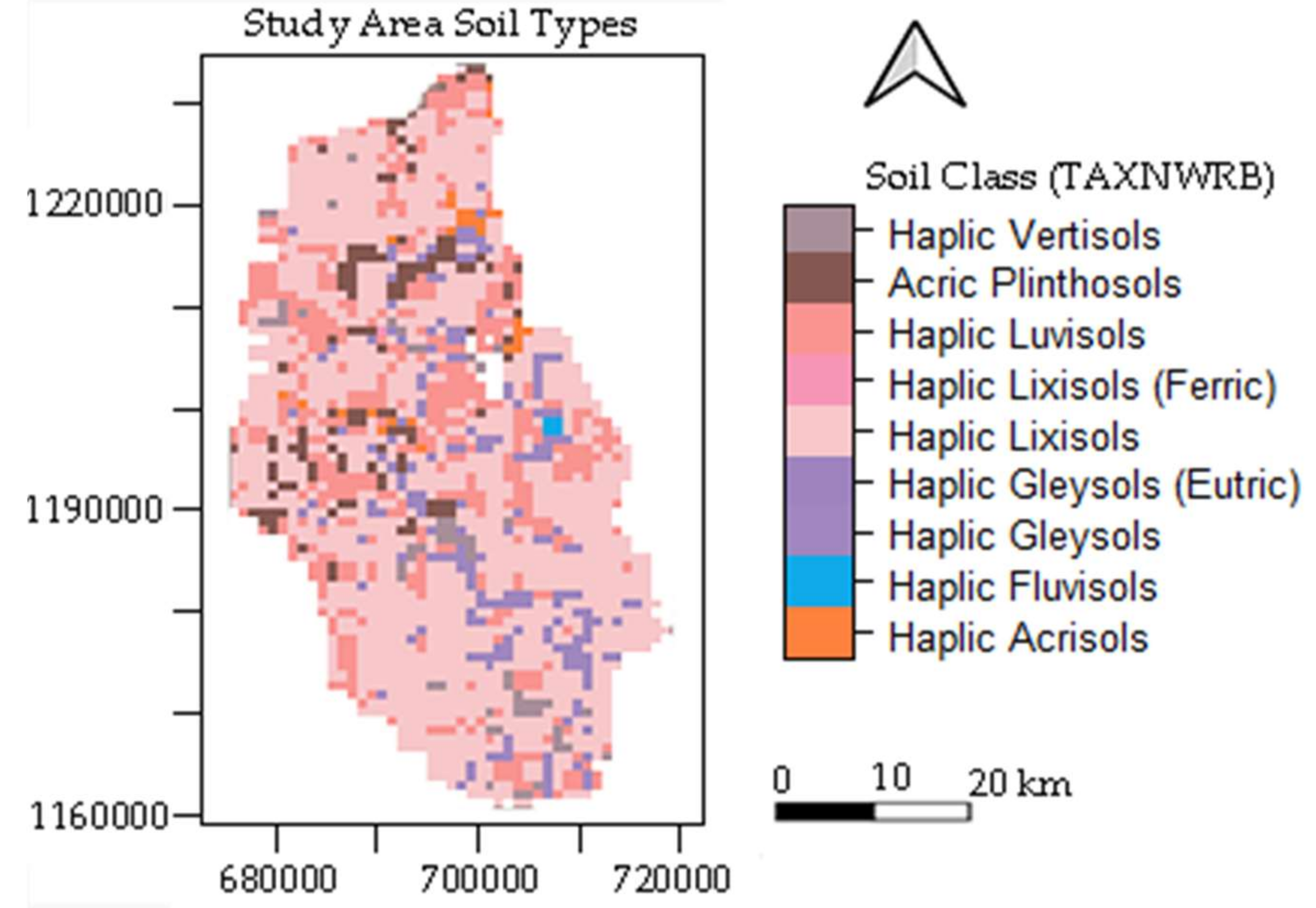
The study area is characterized by about 7 different classes of soils with 9 different soil names (Figure 2). The dominant soil class is Lixisols with the Haplic Lixisols type spanning about 61% of the total study area. Lixisols are characterized by the movement and accumulation of low-activity clays (cation-exchange capacity < 24 cmolc kg−1 clay) and high base saturation (>50%). The dominant soil processes involved in Lixisol formation include argilluviation and biological enrichment of base cations. These soils are often polygenetic and have strong textural differentiation and advanced weathering but with abundant base cycling [60].
2.5. Data from Remote Sensing
ASTER comprises spectral bands, five of which are thermal infrared (TIR), six short-wave-infrared (SWIR), and finally three visible-near-infrared (VNIR) with a ground resolution of 90, 30, as well as 15 m, respectively [61]. ASTER Level 1-T images of the Tono catchment were obtained for two different dates, 20th and 27th of December 2009, and also 17th and 26th December, 2017 and geo-rectified to Zone 30N of the Universal Transverse Mercator projection system (UTM) employing packages in R [62]. Due to the vastness of the research area, images acquired for the two dates of each year were mosaiced into one to cover the entire study area for analysis. The ASTER VNIR radiance was converted to reflectance using scripts written by [63] with modifications by this research to incorporate the TIR bands based on the digital numbers () of the individual ASTER L1 TIR bands, the associated unit conversion coefficients () from the [61], and inversion of the Planck’s radiance function for wavelength based on Equations (1) and (2):
where represents ASTER measured intensity of the spectral radiance (W/m2/sr/µm) obtained from the () values, is the at-sensor brightness temperature of the landcover type in Kelvins, is the Planck’s constant and is given as , is the Boltzmann’s constant and is given as , and is the speed of light in vacuum and is given as . After calculation of the radiance values, reflectance at the top of the atmosphere was calculated for the VNIR bands while at-sensor brightness temperature was computed for the TIR bands based on our modification of the script [63]. Surface reflectance of ASTER bands 2 and 3N was used for the computation of Normalized Difference Vegetation Index (NDVI) using the equation below [64,65,66,67];
where Band 3N is near-infrared and Band 2 is visible red reflectance.
An equation relating the NDVI to the leaf area index (LAI) played a role, and the equation is as follows [68]:
A key input parameter to the modeling process by the TSEB approach is the surface radiometric temperature (. was retrieved using the two-channel algorithms [69] for ASTER TIR bands. The two-channel algorithms [69] implements a linear method for combining the TIR bands of a satellite for the retrieval of surface radiometric temperature. The was then disaggregated to a spatial resolution of 15m to conform to the spatial resolution of the ASTER VNIR using the disaggregate radiometric temperature (Dis) [70] approach and regression kriging. The Dis approach has given satisfactory performance in agricultural setups [71].
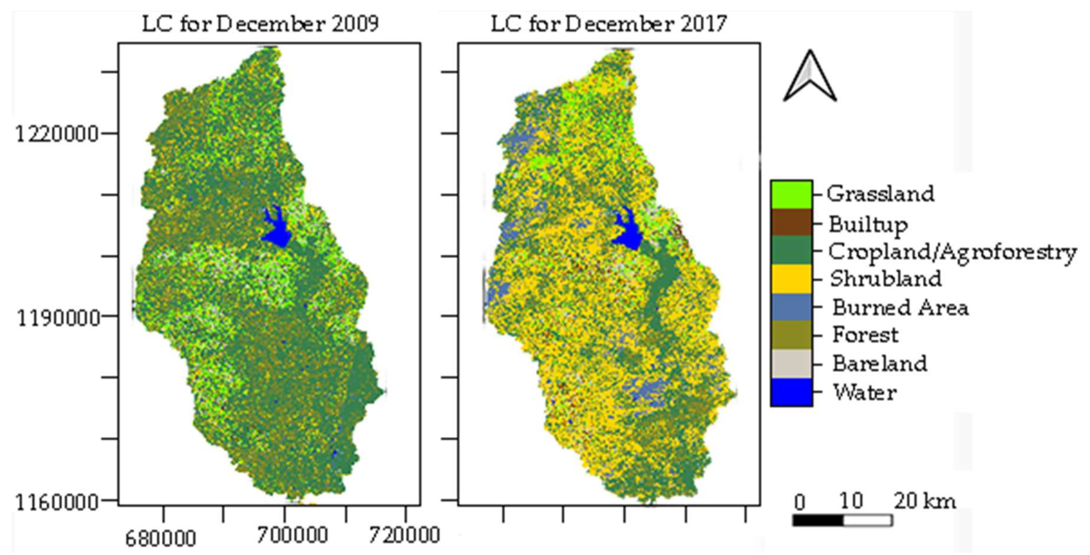
Land use land cover (LULC) maps for the two study periods were generated through a classification of the ASTER L1 T satellite images. Prior to the classification, training, and validation data were obtained by a combination of field survey and digitizing of unique land cover types from Google Earth imagery of December 2017. The digitizing was done by identifying unique pixels using a combination of procedures that hones on the capabilities of Open Foris suites of software collections (Collect and Collect Earth) to identify unique features of the landscape from the December 2017 high-resolution images on Google earth. These sets of data culminated in training sets of eight unique land classes identifiable within the subcategories of the six-land cover classification scheme of the Intergovernmental Panel on Climate Change (IPCC).
2.6. Methods
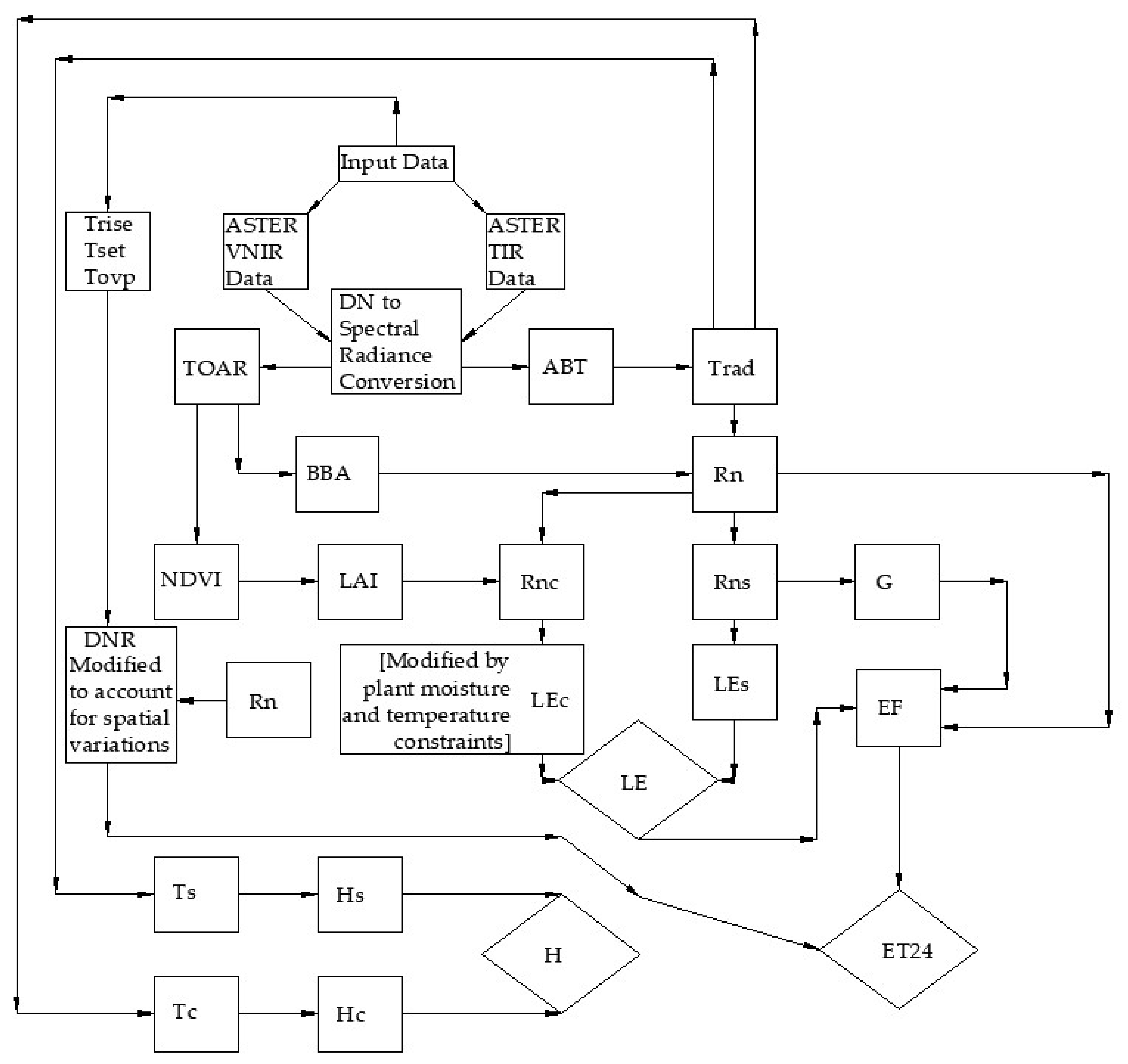
A series of complementary parameters defines the equations that culminate in the novel TSEB algorithm. Some of them are: soil heat flux (G), sensible heat flux (H), latent heat flux (LE), and net radiation (). These parameters are related to each other and to other subsequent parameters in a series of equations that culminates in estimating the daily evapotranspiration from satellite imagery and these equations are detailed in the literature [15,29,32,34,36,37,40,41,71,72,73,74,75,76,77,78,79,80,81,82]. The fundamental equation that forms the basis for the estimation of evapotranspiration from satellite imagery is Equation (5).
Remote sensing images only provide estimated values of the evaporative fraction which has reduced application especially to water resource management, which usually will require daily values of evapotranspiration to allow sufficient and efficient forecasting or irrigation scheduling and other water use metrics. To obtain the daily ET (ET24, mm), this research adopted the extrapolative method of combining the instantaneous evaporative fraction from the ASTER images with the daily radiation, (Rn,24). We integrated the latent heat flux, , over the whole day, using the latent heat of vaporization, L (). We introduced a novel approach to estimate the daily net radiation (Rn,24) component of the modified TSEB algorithm proposed by [15], by estimating the daily net radiation from the ASTER satellite imagery using Equation (6) [46]:
where is the ASTER satellite overpass time over the study area at local time and and are the time of sunrise and sunset, respectively, on the day of the satellite overpass at the study area. Equation (7) was then used to compute the daily ET, (ET24, mm), for the study area:
A flow chart summarizing the major steps toward the novel ET model implementation is shown in Figure 3.
2.7. Supervised LULC Classification of the Satellite Images Using the Random Forest Classifier
The training and validation data gleaned from the field survey and aerial maps were used to conduct a supervised classification, using the algorithm of the Random Forest classifier. The algorithm dips into a set of decision trees to conduct supervised learning. The process involves training the decision trees using a bagging method, but overcomes the challenges of interpretability, a defect typical of the bagging or bootstrap aggregation technique to statistical learning.
The training data was divided into two portions consisting of 70% training data and 30% testing (validation) data. A validation approach for a test of accuracy of the classification was implemented by using the overall accuracy metric, producer and user accuracy, and the kappa coefficient. Overall accuracy is achieved by dividing pixels that were correctly classified by all of the pixels used in the validation [83]. In addition, we generated a confusion matrix and computed the kappa coefficient (κ). The confusion matrix provides for in-depth analysis of the individual accuracy of the different land use classes while the kappa coefficient reveals the accuracy compared to random classifications.
3. Results and Discussion
3.1. Flux Footprint, Footprint Climatology, and Spatial Representativeness of Flux Data
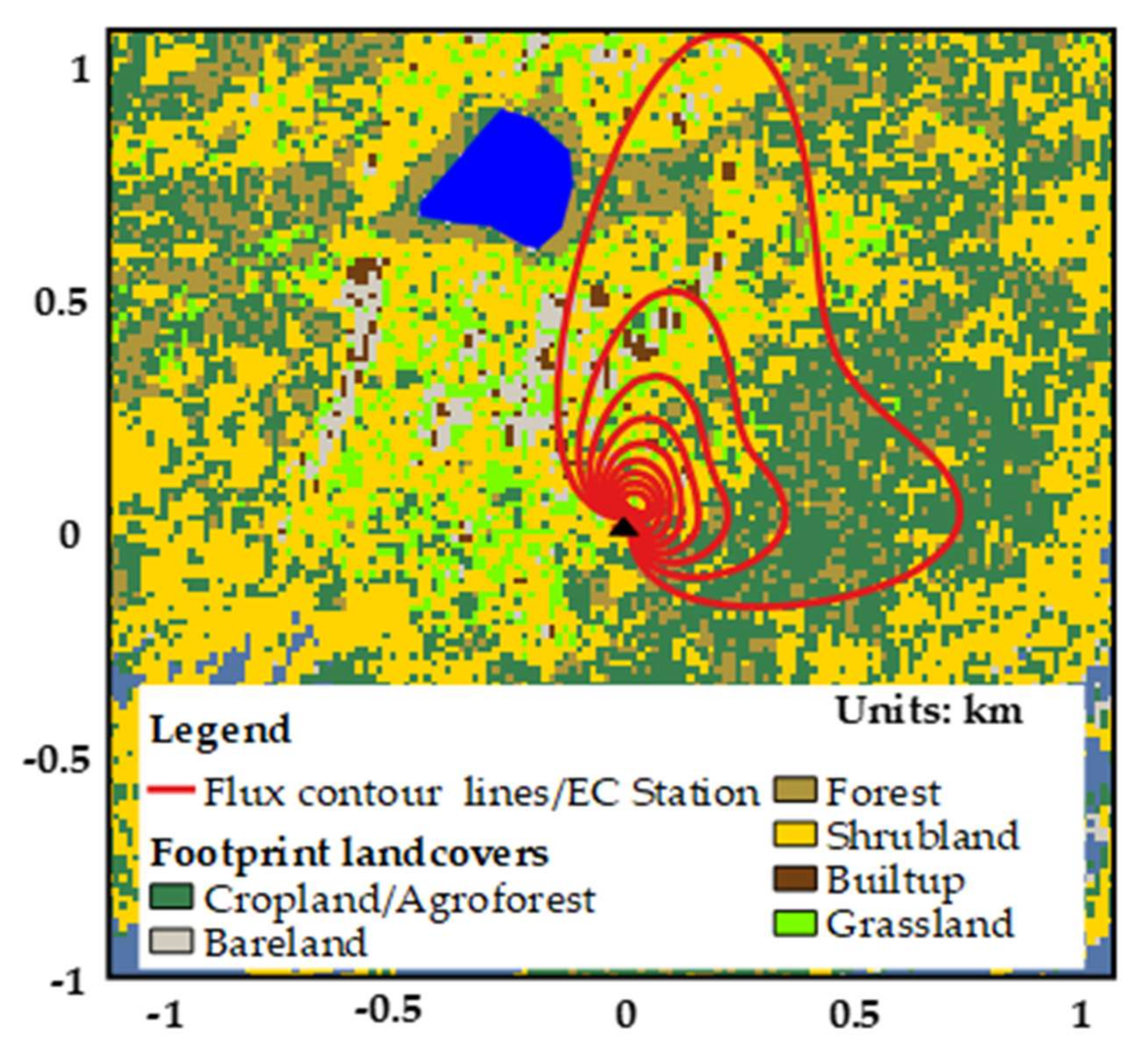
Figure 4 depicts the footprint climatology for the EC station within the catchment of the study area. The black triangle depicts the tower location and measurements taken at a measurement height () of 3.15 m and roughness length () of 0.045 m [84]. Footprint contour lines (red isolines) are shown in steps of 10% from 10% to 90%. In these two-dimensional visualizations, the red contours indicate the three-dimensional topography of the footprint climatologies, with the most influential terrain areas located in the center of the concentric rings. The flux footprint was obtained through a model run online using the [85] FFP tool and superimposed on the landcover map over the study area as shown in the background map.
3.2. Surface Radiometric Temperature
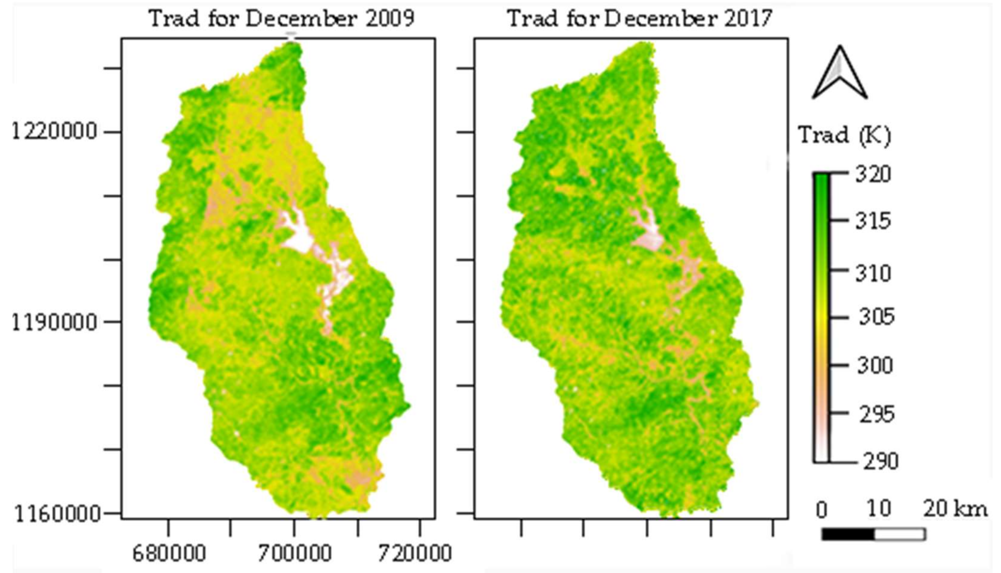
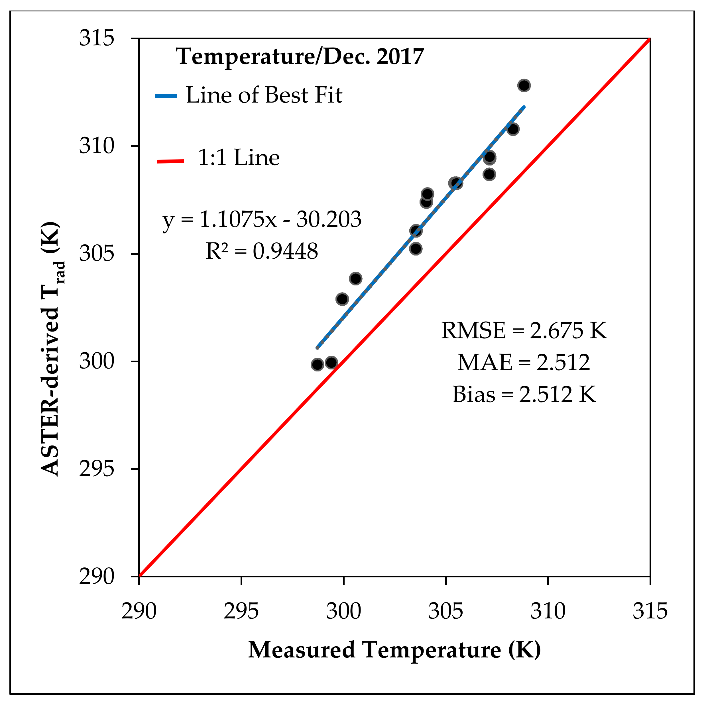
There is no ground-based thermal radiometer device to measure ground-based surface radiometric temperature to compare with the satellite-derived. However, the EC station of the study area is equipped with an open-path infrared gas analyzer (7500A, Li-COR) and a three-dimensional ultrasonic anemometer (CSAT3, Campbell) [48]. These devices measure atmospheric water vapor content, which is a major component in correcting for sonic temperature measured to actual temperature using [86] algorithms and implemented in the TK3 software. Figure 5 presents a spatial distribution of the surface radiometric temperature derived from the ASTER satellite imagery for both December 2017 (Trad for 2017) and December 2009 (Trad for 2009). To investigate the relationship between temperatures, this research compared the surface radiometric temperatures derived from the ASTER satellite imagery for December 2017 with the actual temperatures measured using the ultrasonic anemometer (Figure 6).
Overall, a bias of 2.512 K, root mean squared error (RMSE) of 2.675 K, mean absolute error (MAE) of 2.512, and a determination coefficient of 0.9448 reflects the variations in satellite-derived and ground-based measured temperatures for the study area (Figure 6). was then computed.
3.3. Catchment Evaporation and Potential Evapotranspiration
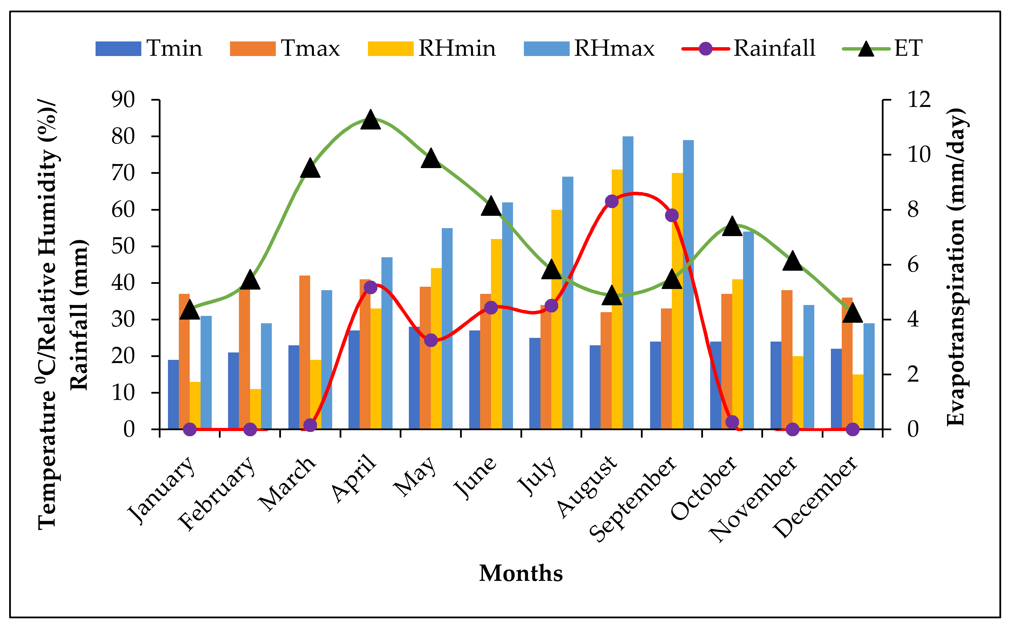
A cloud layer of any magnitude over pixels gives the impression of colder regions, resulting in ET underestimation on account of LST underestimation. Clouds lower the radiative, sensible, and latent energy fluxes. Given these limitations, only clear-sky ASTER L1 T images were acquired for this research to reduce the uncertainty in the estimated ET. We used images for 20th and 27th December 2009 and 17th and 26th December 2017. Images for each corresponding year were mosaiced and clipped to the study area boundary for analysis. Because we desired to compare the results of our satellite base estimated ET with field measured ET from the EC system and EC measurements are unreliable during rainy events and to avoid messy validation results, we only restricted our study to the dry season conditions. On account of this, there was no satellite analysis for ET estimation for the wet season across the different land use types. However, the meteorological data gleaned from the world weather online portal (available at https://www.worldweatheronline.com/) for 2017 helped in estimating mean daily evapotranspiration by the Priestley–Taylor evapotranspiration estimation scheme. The lowest daily ET was recorded in the 12th month (December) at 4.253 mm/d while the highest value occurred in the fourth month (April) at 11.289 mm/d (Figure 7).
3.4. Land Cover Classification
The classification yielded an overall accuracy of 89.49% and a kappa of 84.03% for the 2017 image and an overall accuracy of 82.70% and a kappa of 72.85% for the 2009 satellite image. Table 1 shows the producer and user accuracy for both study periods and Figure 8 shows the corresponding land use map.
3.5. Spatial Variation of Surface Energy Fluxes
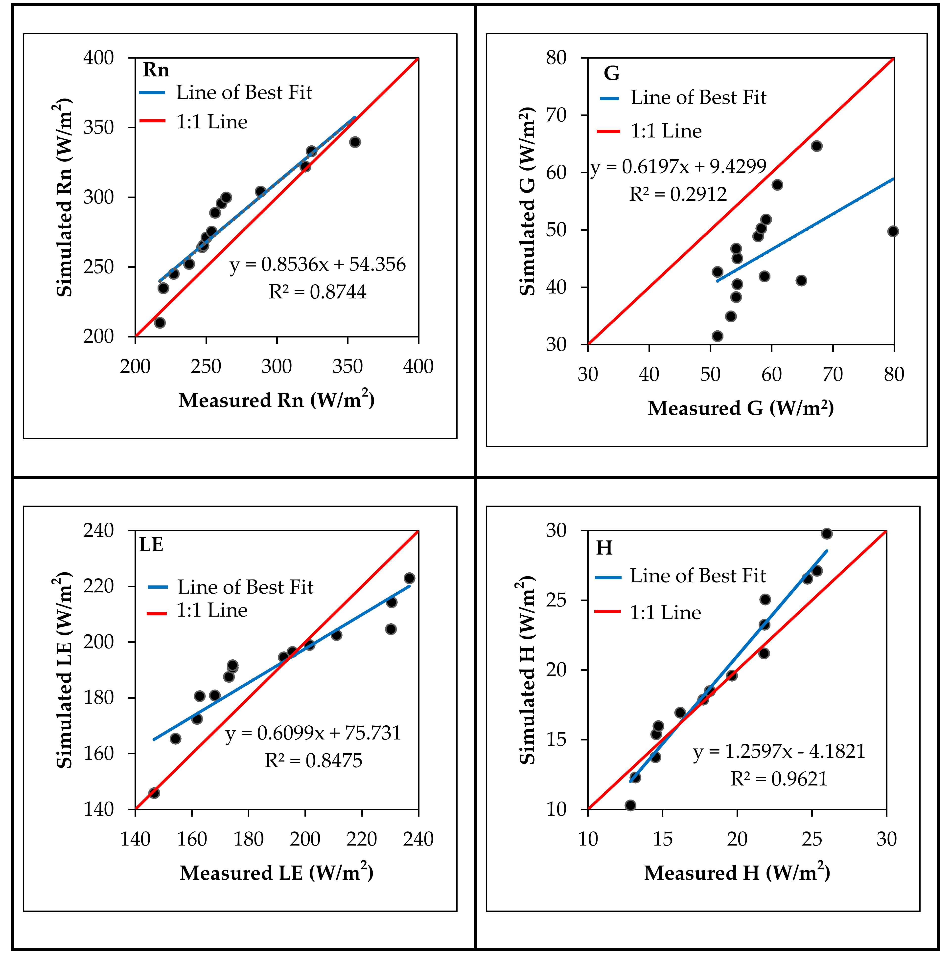
The only direct way by which turbulent heat fluxes are measured is by eddy covariance [55]. Eddy covariance measurements of turbulent fluxes of sensible heat and latent heat in addition to net radiation measurements and soil heat fluxes were conducted on 17th and 26th December 2017, corresponding to the time of clear sky view over the study area for which ASTER satellite imagery was acquired. A statistical analysis to compare the strength of the relationship between measured variables from the eddy covariance system and the simulated are detailed in Table 2 and Figure 9. Of a measured average of 187.5 W/m2, this research simulated an average of 190.1 W/m2 yielding a bias of 2.6 W/m2, root mean squared error (RMSE) of 13.5 W/m2, and mean absolute error (MAE) of 11.5 W/m2 (Table 2) with a coefficient of determination, R2, of approximately 0.85 (Figure 8) for LE. The results indicate that, generally, the satellite estimation of the variables,, , , and and are within the limits of experimental errors, agreeable to direct measurements from the EC tower.
Agreement between ground-based measurements and satellite-derived quantities for , , and offered an opportunity to use the spatially derived satellite estimates of these variables in Equation (7) for deriving spatial variations in over the study area.
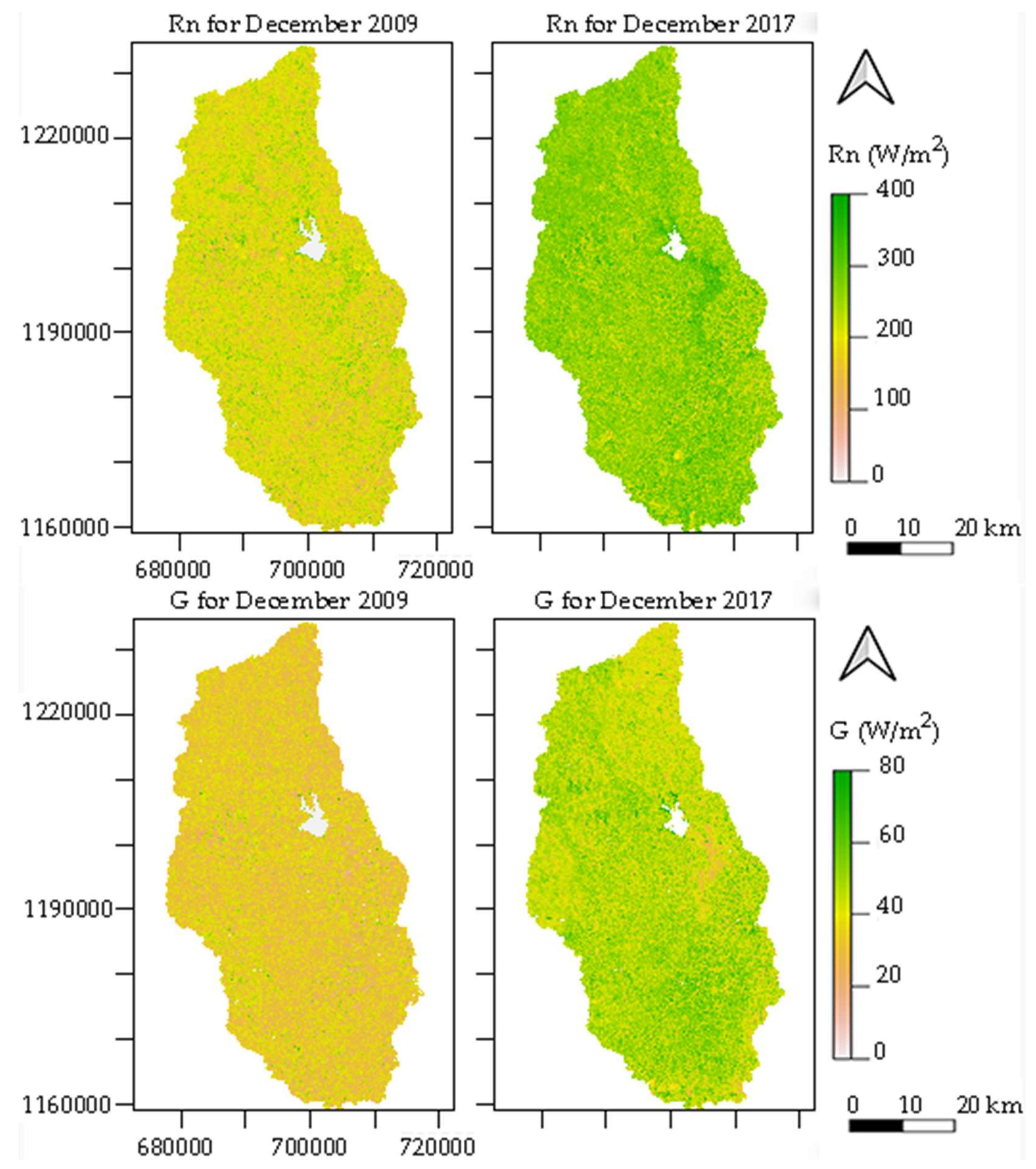
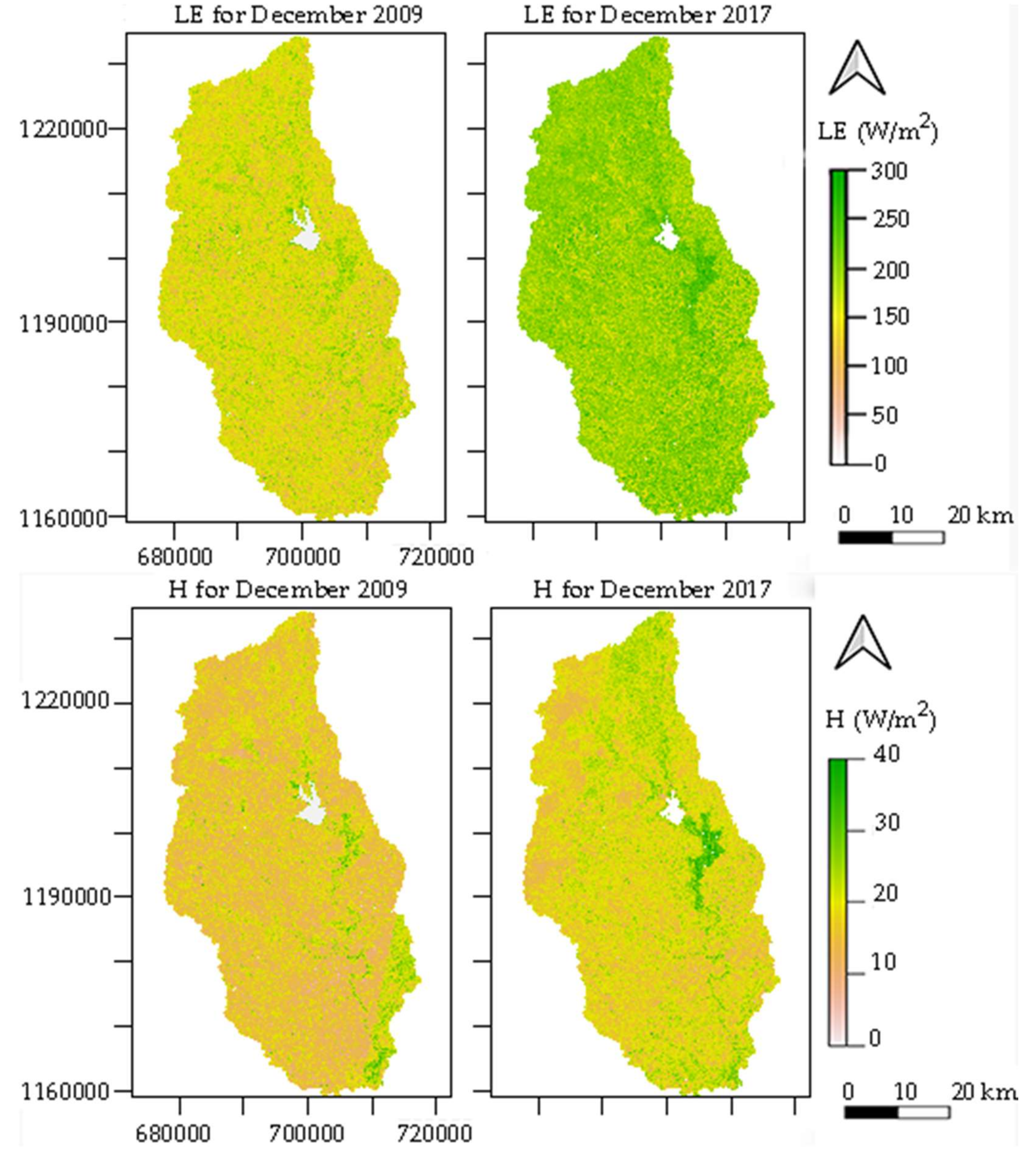
Figure 10 and Figure 11 show the spatiotemporal variation in derived components of the energy balance: , , , and in December 2009 and December 2017. Across the years, the land use types (Figure 8) exhibit a remarkable variation in the energy balance components. Generally, all the surface energy fluxes increased from December 2009 to December 2017. For instance, Rn increased from 210.542 W/m2 in December 2009 to 270.793 W/m2 in December 2017 for the Cropland/Agroforestry land use type (Table 3). LE and H increased from 149.021 W/m2 and 15.375 W/m2 in 2009 to 192.436 W/m2 and 18.712 W/m2 in 2017, respectively, for the Shrubland land use type.
3.6. Partitioning of the Net Radiation (Rn) to LE, H and G Across the Different Land Use Types
The LAI for Cropland/Agroforest land use type was the highest in December 2009 but reduced in December 2017 (Table 4). The Cropland/Agroforest exhibited a higher percentage of Rn converted into LE(LE/Rn), and H(H/Rn) in both 2009 and 2017 than all the other land use types. Except for the Forest landcover type, the LAI and percent of Rn converted to LE(LE/Rn) and H(H/Rn) for Shrubland, Cropland/Agroforestry, and Grassland was higher in December 2009 than in December 2017. The percent of Rn converted to LE(LE/Rn) for the Forest land cover type and the percent of Rn converted to G(G/Rn) for Forest, Shrubland, Cropland/Agroforestry, and Grassland was lower in December 2009 than in December 2017 (Table 4).
The LAI for Cropland/Agroforest decreased from 0.510 cm2cm−2 in December 2009 to 0.410 cm2cm−2 in December 2017 with its percentage of Rn converted to LE (LE/Rn) and H (H/Rn) dropping from 74.714% and 8.217% in December 2009 to 74.509% and 7.945% in December 2017, respectively. These decreases in the LAI, LE/Rn, and H/Rn for Cropland/Agroforest from December 2009 to December 2017 occurred perhaps due to plant senescence and other factors such as water unavailability in the root zone. According to [87], high LAI primarily increases transpiration, contributing then for higher LE/Rn values and vice versa.
Generally, in 2009, the LE/Rn values were in increasing order for the landcover types Shrubland, Forest, Grassland and Cropland/Agroforestry with their corresponding values as 74.098%, 74.316%, 74.656%, and 74.714%. In 2017, the order was Shrubland, Grassland, Forest, Cropland/Agroforestry with corresponding values in increasing order as 73.678%, 74.402%, 74.462%, and 74.509%. The largest value of LE/Rn observed in Cropland/Agroforestry land cover areas is expected because crop reaches higher foliar area providing full soil cover with much higher LAI than the other landcover classes.
Within a class, the percentage of Rn converted into G(G/Rn) and H(H/Rn) varies inversely with LAI and LE/Rn [88]. Physically, this trend is always expected because LE and H fluxes are controlled by soil water availability [89]. On the other hand, G values are controlled by soil water availability and ground cover.
3.7. Daily ET
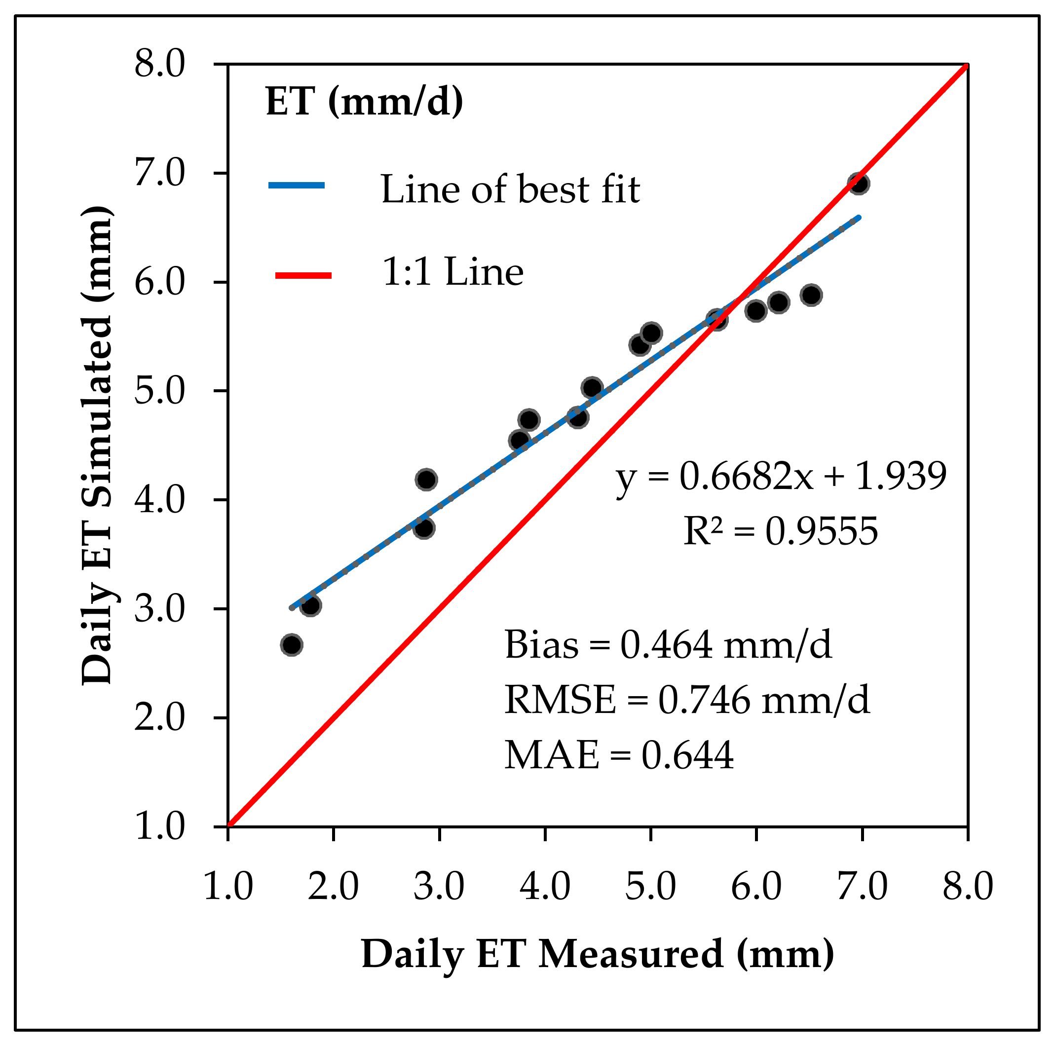
Figure 12 shows a comparison of the simulated ET with the EC tower-based ET measurements. R2 = 0.9555, MAE = 0.644, RMSE = 0.746 mm/d, and bias = 0.966 mm/d. Generally, there is an agreement between simulated and EC tower-based measurements for the study area. The predicted evapotranspiration closely matched the observations in terms of a high degree of fit and low bias, although there was a slight overestimation of daily ET. We present below possible causes.
Simulated ET in most cases was higher than ET measured at the EC station (Figure 11). Apart from the Tono reservoir, a series of other small earth dams and dugouts (containing standing water) are dotted around, within the catchment. Standing water affects landscape moisture which in turn affects ET. The activity of ET is also affected by insolation. ET is a conglomerate of multiple environmental factors including the landcover, ambient conditions of the environment, phenological stage, life history, and vegetation condition. An interplay contributed in part by the magnitude of each of these factors, determines how high or low the ET of a segment of a landscape would be revealed. Simulated ET in most cases was higher than ET measured at the EC station (Figure 11). A reference to Figure 3 indicates that the landcover types within the footprint area of the EC station were Cropland/Agroforestry, Bareland, Forest, Shrubland, Builtup, and Grassland. Apart from the reduced percentage by area of these flux tower footprint landcovers, they also constitute only six out of the eight landcover types (Figure 7) identified by this study. The reason most of the measured ET is lower than the simulated ET is attributable to the unaccounted ET contribution of water areas by the footprint of the EC tower due to reduced moisture in the landscape within the footprint area.
3.8. Spatial Distribution of Daily ET
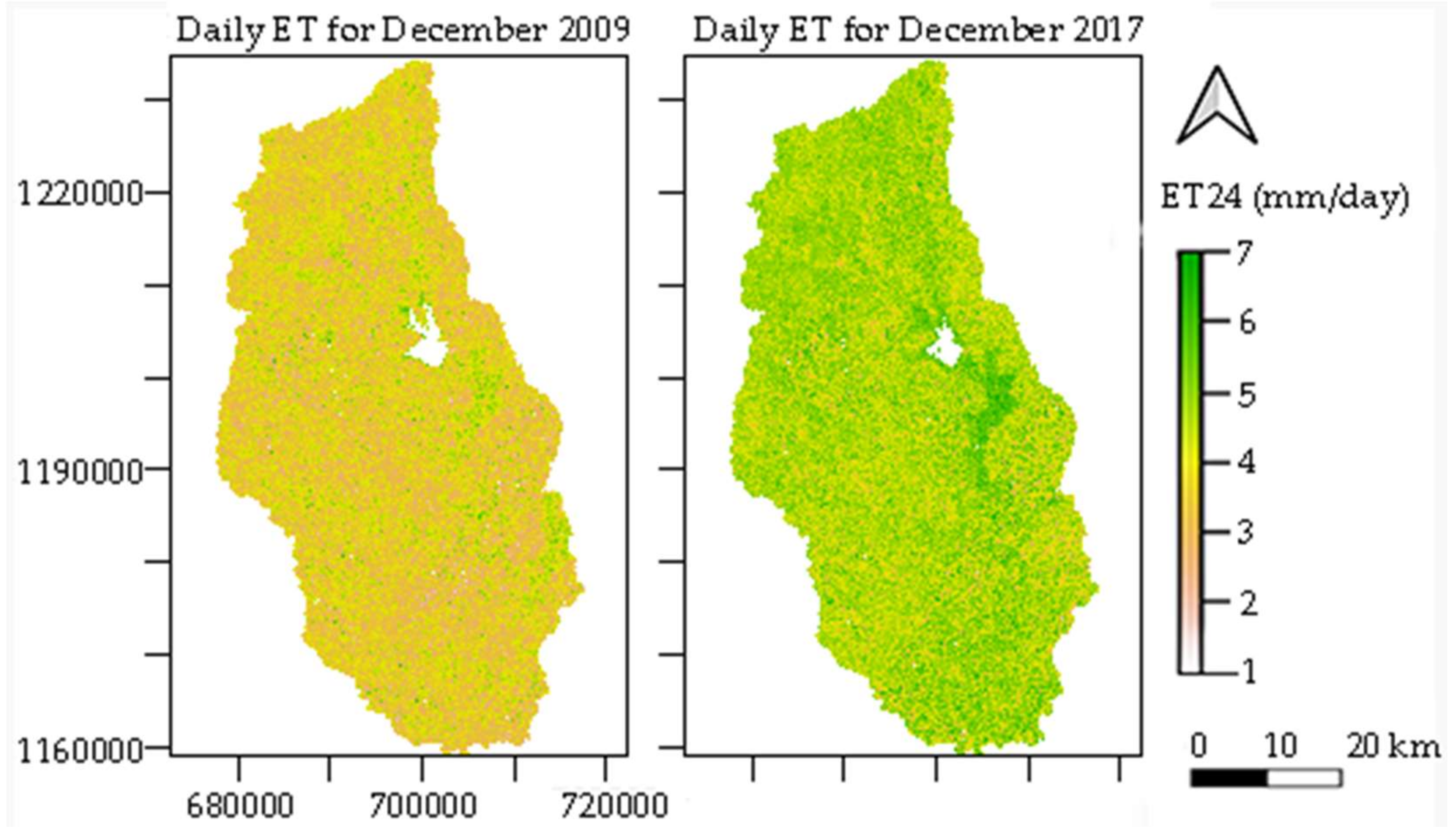
Figure 13 shows maps of the daily ET for the two scenario dates, December 2017 and December 2009. The ET maps for the two days indicate both temporal and spatial variations. Generally, ET for December 2017 was higher than that for December 2009. ET is characteristically multivariate, influenced by a plethora of factors that are inter-connected, including landcover type, available energy, humidity gradient, wind speed, available water, soil characteristics, and vegetation architecture. We identified eight landcover types (Figure 8) in the Tono watershed and each of these landcover types have a distinct contribution to the catchment ET. With a 0.063% increase in water areas in December 2017 (Table 1), there will be more moisture in the landscape to enhance ET. The vegetations identified are Forest and Shrubland, Cropland/Agroforest and Grassland. There was about a 34% increase in the Shrubland area in December 2017 (Table 1). A strong relationship exists between microclimate and vegetation structure [90]. First, plant-canopies intercept incoming solar radiation, thereby limiting energy transmission to the soil below the plants. The amount of the intercepted solar radiation the plant canopy can absorb depends on the leaf area index (LAI) (Table 4). Secondly, plant-canopies absorb some amount of momentum from the surrounding air and so wind speed reduces with depth within the plant canopy [90]. The canopy structure of the catchment is sparse in both December 2009 and 2017, since in both years, the LAI is less than one (Table 4). This results in an increase in air temperature near the ground as the turbulent mixing conducts the hot air formed at the top of the canopy to the ground below. However, comparatively, the LAI for all the vegetation types was higher in December 2009 than in December 2017, implying that, more hot air was conducted to the ground below in December 2017 than in December 2009. This state results in a slight increase in air temperature in December 2017 than in December 2009. Air temperature is known to have a direct link with evapotranspiration. Finally, the water vapor holding capacity of air is influenced by air temperature. Low LAI canopies offer higher air temperatures, resulting in larger vapor pressure deficit (VPD) and lower relative humidity. VPD has a direct link with ET. Therefore, given the sparser canopy structure of the December 2017 vegetation as evidenced by the LAI, it is not surprising that the ET is higher in December 2017 than December 2009.
3.9. ET Variations per Land Use Type
Water areas exhibited the highest ET value for both study periods, with ET values in the same range (Table 5). However, the ET for water areas in December 2017 was higher (5.28 mm/d) than that of December 2009 (4.486 mm/d). The lowest ET in December 2009 was obtained from Shrubland areas (3.576 mm/d) while for December 2017, it was in Burned areas (4.502 mm/d). This trend of values is similar to the findings of [91,92]. The mean ET across the different land use/cover types was 4.271 mm/d with a coefficient of variation (CV) of 14.807%. The range of CV for ET across the different land use/cover types is 10.415–24.478%, falling within the ranges reported by [92] (5−47%), [22] (18−77%), and [91] (6−59%). Areas with water have the highest CV (24.478%) for December 2009 while Cropland/Agroforest areas have the highest CV (12.365%) in December 2017. Our simulated CV (11.762–24.478%) for water areas is within the range reported by [91] (6–30%) for water bodies. Overall, the novel TSEB as applied on the ASTER Level 1-T satellite imagery facilitated in providing spatial variations in turbulent heat fluxes across different land use types over the tropical savanna climate of the Northern Ghana and Southern Burkina Faso.
4. Conclusions
The study estimated surface energy fluxes across different land use types using the novel TSEB model and ASTER satellite imagery over a tropical savanna climatic region for the first time. The ASTER images which provided input data for the novel TSEB model were collected over the catchment area of the Tono Reservoir which lies within the Upper East Region of Ghana and Southern Burkina Faso. Due to the negative influence that a cloud cover has on the quality of estimated variables, the study only used satellite images with no cloud cover for analysis. Variables estimated from the satellite images based on the novel TSEB algorithm were validated agreeable with their corresponding field measured data from the eddy covariance systems within the study area established by the WASCAL. Based on the agreeableness between simulated and observed , was simulated and consequently , , and , which eventually provided ample basis for predicting the spatial variations in . is a significant component in water resources management within watersheds.
Mean ET varied from 3.576 to 4.486 (mm/d) for December 2009 while from 4.502 to 5.280 (mm/d) for December 2017 across the different land use/cover classes. Water areas exhibited the highest mean ET value in both 2009 and 2017, though with an increasing trend from 4.486 to 5.280 (mm/d), respectively. The range of CVs for ET was within 10.415–24.478% across the different land use/cover types for the catchment. The ET for December 2017 was generally higher than that for December 2009. This research paves an outlet to reliably apply the novel TSEB algorithm on satellite imagery for the estimation of turbulent heat fluxes across different land use types in tropical savanna climatic regions where it may be a challenge to carry out rigorous costly field measurements.
Author Contributions
Conceptualization, A.A. and M.J.; Funding acquisition, M.J.; Supervision, M.J.; Writing—Original draft preparation, A.A.; Writing—Review and editing, A.A. All authors have read and agreed to the published version of the manuscript.
Funding
This study was supported by the National Natural Science Foundation of China (Nos. U1403282, and 41672246).
Acknowledgments
The micrometeorological flux data was provided by the West African Science Service Center on Climate Change and Adapted Land Use (WASCAL) at Ghana/Burkina Faso (https://www.wascal.org/). We are thankful to Samuel Guug for providing the shapefiles of the study area boundary. We are grateful to the academic editor and all the anonymous reviewers for their valuable comments and critical feedbacks.
Conflicts of Interest
The authors declare that no conflicts of interest exist.
Acronyms
| 1S | One-source |
| 2S | Dual-source |
| ABT | At-sensor brightness temperature |
| BBA | Broad-band albedo |
| DNR | Daily net radiation |
| EC | Eddy covariance |
| EF | Evaporative fraction |
| ET | Evapotranspiration |
| ET24 | Daily evapotranspiration |
| FAPAR | Fraction of Absorbed Photosynthetically Active Radiation |
| fg | Fraction of green canopy |
| FIPAR | Fraction of Intercepted Photosynthetically Active Radiation |
| fM | Plant moisture constraints |
| G | Soil heat flux |
| H | Sensible heat flux |
| Hc | Canopy sensible heat flux |
| Hs | Soil sensible heat flux |
| LAI | Leaf area index |
| LE | Latent heat flux |
| LEc | Canopy latent heat flux |
| LEs | Soil latent heat flux |
| LSE | Land surface emissivity |
| NDVI | Normalized difference vegetation index |
| Rn | Net radiation |
| Rnc | Canopy net radiation |
| Rns | Soil net radiation |
| Tc | Canopy temperature |
| TOAR | Top of atmosphere reflectance |
| Tovp | Time of satellite overpass |
| Trad | Land surface radiometric temperature |
| Trise | Time of sunrise |
| Ts | Soil temperature |
| TSEB | Two-source energy balance |
| Tset | Time of sunset |
| WASCAL | West African Science Service Center on Climate Change and Adapted Land Use |
References
- Ahmadi, B.; Ahmadalipour, A.; Tootle, G.; Hamid, M. Remote Sensing of Water Use Efficiency and Terrestrial Drought Recovery across the Contiguous United States. Remote Sens. 2019, 11, 731. [Google Scholar] [CrossRef] [Green Version]
- Yu, Z.; Wang, J.; Liu, S.; Rentch, J.S.; Sun, P.; Lu, C. Global gross primary productivity and water use efficiency changes under drought stress. Environ. Res. Lett. 2017, 12, 014016. [Google Scholar] [CrossRef] [Green Version]
- Hasenmueller, E.A.; Criss, R.E. Water Balance Estimates of Evapotranspiration Rates in Areas with Varying Land Use. In Evapotranspiration—An Overview; Alexandris, S.G., Ed.; IntechOpen: London, UK, 2013; p. 22. [Google Scholar] [CrossRef] [Green Version]
- Katul, G.; Novick, K. Evapotranspiration. In Encyclopedia of Inland Waters; Likens, G.E., Ed.; Academic Press: Oxford, UK, 2009; pp. 661–667. [Google Scholar] [CrossRef]
- Merlin, O.; Chirouze, J.; Olioso, A.; Jarlan, L.; Chehbouni, G.; Boulet, G. An image-based four-source surface energy balance model to estimate crop evapotranspiration from solar reflectance/thermal emission data (SEB-4S). Agric. For. Meteorol. 2014, 184, 188–203. [Google Scholar] [CrossRef] [Green Version]
- Nouri, H.; Beecham, S.; Kazemi, F.; Hassanli, A.M.; Anderson, S. Remote sensing techniques for predicting evapotranspiration from mixed vegetated surfaces. Hydrol. Earth Syst. Sci. Discuss. 2013, 10, 3897–3925. [Google Scholar] [CrossRef]
- Verstraeten, W.; Veroustraete, F.; Feyen, J. Assessment of Evapotranspiration and Soil Moisture Content Across Different Scales of Observation. Sensors 2008, 8, 70–117. [Google Scholar] [CrossRef] [Green Version]
- Bastiaanssen, W.G.M. SEBAL-based sensible and latent heat fluxes in the irrigated Gediz Basin, Turkey. J. Hydrol. 2000, 229, 87–100. [Google Scholar] [CrossRef]
- Kustas, W.P.; Norman, J.M. Use of remote sensing for evapotranspiration monitoring over land surfaces. Hydrol. Sci. J. 1996, 41, 495–516. [Google Scholar] [CrossRef]
- Mu, Q.; Heinsch, F.A.; Zhao, M.; Running, S.W. Development of a global evapotranspiration algorithm based on MODIS and global meteorology data. Remote Sens. Environ. 2007, 111, 519–536. [Google Scholar] [CrossRef]
- Wang, K.; Wang, P.; Li, Z.; Cribb, M.; Sparrow, M. A Simple Method to Estimate Actual Evapotranspiration from A Combination of Net Radiation, Vegetation Index, and Temperature. J. Geophys. Res. 2007, 112, D15107. [Google Scholar] [CrossRef]
- Bahir, M.; Boulet, G.; Olioso, A.; Rivalland, V.; Gallego-Elvira, B.; Mira, M.; Rodriguez, J.-C.; Jarlan, L.; Merlin, O. Evaluation and Aggregation Properties of Thermal Infra-Red-Based Evapotranspiration Algorithms from 100 m to the km Scale over a Semi-Arid Irrigated Agricultural Area. Remote Sens. 2017, 9, 1178. [Google Scholar] [CrossRef] [Green Version]
- Cheng, J.; Kustas, W.P. Using Very High Resolution Thermal Infrared Imagery for More Accurate Determination of the Impact of Land Cover Differences on Evapotranspiration in an Irrigated Agricultural Area. Remote Sens. 2019, 11, 613. [Google Scholar] [CrossRef] [Green Version]
- Ma, W.; Hafeez, M.; Ishikawa, H.; Ma, Y. Evaluation of SEBS for estimation of actual evapotranspiration using ASTER satellite data for irrigation areas of Australia. Theor. Appl. Climatol. 2013, 112, 609–616. [Google Scholar] [CrossRef]
- Zhuang, Q.; Wu, B. Estimating Evapotranspiration from an Improved Two-Source Energy Balance Model Using ASTER Satellite Imagery. Water 2015, 7, 6673–6688. [Google Scholar] [CrossRef] [Green Version]
- Bawazir, A.S.; Samani, Z.; Bleiweiss, M.; Skaggs, R.; Schmugge, T. Using ASTER satellite data to calculate riparian evapotranspiration in the Middle Rio Grande, New Mexico. Int. J. Remote Sens. 2009, 30, 5593–5603. [Google Scholar] [CrossRef]
- Zhang, Y.-K.; Schilling, K. Effects of Land Cover on Water Table, Soil Moisture, Evapotranspiration, and Groundwater Recharge: A Field Observation and Analysis. J. Hydrol. 2006, 319, 328–338. [Google Scholar] [CrossRef]
- Dunn, S.M.; Mackay, R. Spatial variation in evapotranspiration and the influence of land use on catchment hydrology. J. Hydrol. 1995, 171, 49–73. [Google Scholar] [CrossRef]
- Gerten, D.; Schaphoff, S.; Haberlandt, U.; Lucht, W.; Sitch, S. Terrestrial vegetation and water balance—Hydrological evaluation of a dynamic global vegetation model. J. Hydrol. 2004, 286, 249–270. [Google Scholar] [CrossRef]
- Senay, G.B.; Bohms, S.; Singh, R.K.; Gowda, P.H.; Velpuri, N.M.; Alemu, H.; Verdin, J.P. Operational Evapotranspiration Mapping Using Remote Sensing and Weather Datasets: A New Parameterization for the SSEB Approach. JAWRA J. Am. Water Resour. Assoc. 2013, 49, 577–591. [Google Scholar] [CrossRef] [Green Version]
- Senay, G.B.; Budde, M.; Verdin, J.P.; Melesse, A.M. A Coupled Remote Sensing and Simplified Surface Energy Balance Approach to Estimate Actual Evapotranspiration from Irrigated Fields. Sensors 2007, 7, 979–1000. [Google Scholar] [CrossRef] [Green Version]
- Allen, R.G.; Tasumi, M.; Trezza, R. Satellite-Based Energy Balance for Mapping Evapotranspiration with Internalized Calibration (METRIC)-Model. J. Irrig. Drain. Eng. 2007, 133, 380–394. [Google Scholar] [CrossRef]
- Su, Z. The Surface Energy Balance System (SEBS) for estimation of turbulent heat fluxes. Hydrol. Earth Syst. Sci. 2002, 6, 85–100. [Google Scholar] [CrossRef]
- Roerink, G.J.; Su, Z.; Menenti, M. S-SEBI: A simple remote sensing algorithm to estimate the surface energy balance. Phys. Chem. Earth Part B Hydrol. Ocean. Atmos. 2000, 25, 147–157. [Google Scholar] [CrossRef]
- Bastiaanssen, W.G.M.; Menenti, M.; Feddes, R.A.; Holtslag, A.A.M. A remote sensing surface energy balance algorithm for land (SEBAL). 1. Formulation. J. Hydrol. 1998, 212–213, 198–212. [Google Scholar] [CrossRef]
- Paul, G.; Gowda, P.H.; Vara Prasad, P.V.; Howell, T.A.; Aiken, R.M.; Neale, C.M.U. Investigating the influence of roughness length for heat transport (zoh) on the performance of SEBAL in semi-arid irrigated and dryland agricultural systems. J. Hydrol. 2014, 509, 231–244. [Google Scholar] [CrossRef]
- Gokmen, M.; Vekerdy, Z.; Verhoef, A.; Verhoef, W.; Batelaan, O.; van der Tol, C. Integration of soil moisture in SEBS for improving evapotranspiration estimation under water stress conditions. Remote Sens. Environ. 2012, 121, 261–274. [Google Scholar] [CrossRef]
- Yang, Y.; Su, H.; Zhang, R.; Tian, J.; Li, L. An enhanced two-source evapotranspiration model for land (ETEML): Algorithm and evaluation. Remote Sens. Environ. 2015, 168, 54–65. [Google Scholar] [CrossRef]
- Norman, J.M.; Kustas, W.P.; Prueger, J.H.; Diak, G.R. Surface flux estimation using radiometric temperature: A dual-temperature-difference method to minimize measurement errors. Water Resour. Res. 2000, 36, 2263–2274. [Google Scholar] [CrossRef] [Green Version]
- Mecikalski, J.R.; Diak, G.R.; Anderson, M.C.; Norman, J.M. Estimating Fluxes on Continental Scales Using Remotely Sensed Data in an Atmospheric–Land Exchange Model. J. Appl. Meteorol. 1999, 38, 1352–1369. [Google Scholar] [CrossRef]
- Anderson, M.C.; Norman, J.M.; Diak, G.R.; Kustas, W.P.; Mecikalski, J.R. A two-source time-integrated model for estimating surface fluxes using thermal infrared remote sensing. Remote Sens. Environ. 1997, 60, 195–216. [Google Scholar] [CrossRef]
- Norman, J.M.; Kustas, W.P.; Humes, K.S. Source approach for estimating soil and vegetation energy fluxes in observations of directional radiometric surface temperature. Agric. For. Meteorol. 1995, 77, 263–293. [Google Scholar] [CrossRef]
- Lhomme, J.P.; Chehbouni, A. Comments on dual-source vegetation–atmosphere transfer models. Agric. For. Meteorol. 1999, 94, 269–273. [Google Scholar] [CrossRef]
- Sánchez, J.M.; Kustas, W.P.; Caselles, V.; Anderson, M.C. Modelling surface energy fluxes over maize using a two-source patch model and radiometric soil and canopy temperature observations. Remote Sens. Environ. 2008, 112, 1130–1143. [Google Scholar] [CrossRef]
- Anderson, M.; Norman, J.; Kustas, W.; Houborg, R.; Starks, P.; Agam, N. A thermal-based remote sensing technique for routine mapping of land-surface carbon, water and energy fluxes from field to regional scales. Remote Sens. Environ. 2008, 112, 4227–4241. [Google Scholar] [CrossRef]
- Long, D.; Singh, V.P. A Two-source Trapezoid Model for Evapotranspiration (TTME) from satellite imagery. Remote Sens. Environ. 2012, 121, 370–388. [Google Scholar] [CrossRef]
- Morillas, L.; Villagarcía, L.; Domingo, F.; Nieto, H.; Uclés, O.; García, M. Environmental factors affecting the accuracy of surface fluxes from a two-source model in Mediterranean drylands: Upscaling instantaneous to daytime estimates. Agric. For. Meteorol. 2014, 189–190, 140–158. [Google Scholar] [CrossRef]
- Kustas, W.P.; Norman, J.M. A two-source approach for estimating turbulent fluxes using multiple angle thermal infrared observations. Water Resour. Res. 1997, 33, 1495–1508. [Google Scholar] [CrossRef]
- Gonzalez-Dugo, M.P. A comparison of operational remote sensing-based models for estimating crop evapotranspiration. Agric. For. Meteorol. 2009, 149, 1843–1853. [Google Scholar] [CrossRef]
- Li, F.; Kustas, W.P.; Prueger, J.H.; Neale, C.M.U.; Jackson, T.J. Utility of Remote Sensing–Based Two-Source Energy Balance Model under Low- and High-Vegetation Cover Conditions. J. Hydrometeorol. 2005, 6, 878–891. [Google Scholar] [CrossRef]
- Fisher, J.B.; Tu, K.P.; Baldocchi, D.D. Global estimates of the land–atmosphere water flux based on monthly AVHRR and ISLSCP-II data, validated at 16 FLUXNET sites. Remote Sens. Environ. 2008, 112, 901–919. [Google Scholar] [CrossRef]
- WikimediaCommonsContributors. China Map of Köppen Climate Classification; 14 February 2018 ed.. Wikimedia Commons—The Free Media Repository, 2018. Available online: https://commons.wikimedia.org/w/index.php?title=File:China_map_of_K%C3%B6ppen_climate_classification.svg&oldid=287152692 (accessed on 7 February 2020).
- Beck, H.E.; Zimmermann, N.E.; McVicar, T.R.; Vergopolan, N.; Berg, A.; Wood, E.F. Present and future Köppen-Geiger climate classification maps at 1-km resolution. Sci. Data 2018, 5, 180214. [Google Scholar] [CrossRef] [Green Version]
- Krishna, S.; Manavalan, P.; Rao, P. Estimation of Net Radiation using satellite based data inputs. ISPRS Int. Arch. Photogramm. Remote Sens. Spat. Inf. Sci. 2014, XL-8, 307–313. [Google Scholar] [CrossRef] [Green Version]
- WikimediaCommonsContributors. Ghana Map of Köppen Climate Classification. Available online: https://commons.wikimedia.org/w/index.php?title=File:Ghana_map_of_K%C3%B6ppen_climate_classification.svg&oldid=287173920 (accessed on 7 February 2020).
- Bisht, G.; Bras, R.L. Estimation of Net Radiation From the Moderate Resolution Imaging Spectroradiometer Over the Continental United States. IEEE Trans. Geosci. Remote Sens. 2011, 49, 2448–2462. [Google Scholar] [CrossRef]
- Nicholson, S.E. The West African Sahel: A Review of Recent Studies on the Rainfall Regime and Its Interannual Variability. ISRN Meteorol. 2013, 2013, 32. [Google Scholar] [CrossRef]
- Bliefernicht, J.; Berger, S.; Salack, S.; Guug, S.; Hingerl, L.; Heinzeller, D.; Mauder, M.; Steinbrecher, R.; Steup, G.; Bossa, A.Y.; et al. The WASCAL Hydrometeorological Observatory in the Sudan Savanna of Burkina Faso and Ghana. Vadose Zone J. 2018, 17. [Google Scholar] [CrossRef] [Green Version]
- Alhassan, A.; Agyare, W.A.; Asante, C.Y. Impact of Landuse Changes on Soil Erosion and Sedimentation in the Tono Reservoir Watershed Using GeoWEPP Model. Int. J. Irrig. Agric. Dev. 2018, 1, 106–119. [Google Scholar]
- Forkuor, G.; Conrad, C.; Thiel, M.; Zoungrana, B.; Tondoh, J. Multiscale Remote Sensing to Map the Spatial Distribution and Extent of Cropland in the Sudanian Savanna of West Africa. Remote Sens. 2017, 9, 839. [Google Scholar] [CrossRef] [Green Version]
- Ouedraogo, I.; Savadogo, P.; Tigabu, M.; Cole, R.; Odén, P.C.; Ouadba, J.-M. Is rural migration a threat to environmental sustainability in Southern Burkina Faso? Land Degrad. Dev. 2009, 20, 217–230. [Google Scholar] [CrossRef]
- Quansah, E.; Mauder, M.; Balogun, A.A.; Amekudzi, L.K.; Hingerl, L.; Bliefernicht, J.; Kunstmann, H. Carbon dioxide fluxes from contrasting ecosystems in the Sudanian Savanna in West Africa. Carbon Balance Manag. 2015, 10, 1. [Google Scholar] [CrossRef] [Green Version]
- Bliefernicht, J.; Kunstmann, H.; Hingerl, L.; Rummler, T.; Andresen, S.; Mauder, M.; Steinbrecher, R.; Frieß, R.; Gochis, D.; Gessner, U.; et al. Field and Simulation Experiments for Investigating Regional Land-Atmosphere Interactions in West Africa: Experimental Set-up and First Results; IAHS Publ.: Gothenburg, Sweden, 2013. [Google Scholar]
- Fratini, G.; Mauder, M. Towards a consistent eddy-covariance processing: An intercomparison of EddyPro and TK3. Atmos. Meas. Tech. 2014, 7, 2273–2281. [Google Scholar] [CrossRef] [Green Version]
- Mauder, M.; Foken, T. Documentation and Instruction Manual of the Eddy-Covariance Software Package TK3; Universität Bayreuth, Abteilung Mikrometeorologie: Bayreuth, Germany, 2011. [Google Scholar]
- Mauder, M.; Foken, T.; Clement, R.; Elbers, J.A.; Eugster, W.; Grünwald, T.; Heusinkveld, B.; Kolle, O. Quality control of CarboEurope flux data? Part 2: Inter-comparison of eddy-covariance software. Biogeosciences 2008, 5, 451–462. [Google Scholar] [CrossRef] [Green Version]
- Kaimal, J.C.; Finnigan, J.J. Atmospheric Boundary Layer Flows: Their Structure and Measurement; Oxford University Press: New York, NY, USA, 1994. [Google Scholar]
- Foken, T.; Leuning, R.; Oncley, S.R.; Mauder, M.; Aubinet, M. Corrections and Data Quality Control. In Eddy Covariance: A Practical Guide to Measurement and Data Analysis; Aubinet, M., Vesala, T., Papale, D., Eds.; Springer: Dordrecht, The Netherlands, 2012; pp. 85–131. [Google Scholar] [CrossRef]
- Foken, T.; Wichura, B. Tools for quality assessment of surface-based flux measurements. Agric. Forest Meteorol. 1996, 78, 83–105. [Google Scholar] [CrossRef]
- FAO; ITPS. Status of the World’s Soil Resources (SWSR)—Main Report; Food and Agriculture Organization of the United Nations and Intergovernmental Technical Panel on Soils: Rome, Italy, 2015. [Google Scholar]
- Michael, A.; Simon, H.; Bhaskar, R. ASTER Users Handbook Version 2; Jet Propulsion Laboratory/California Institute of Technology: Pasadena, CA, USA, 1998. [Google Scholar]
- R-Core-Team. R: A Language and Environment for Statistical Computing; R Foundation for Statistical Computing: Vienna, Austria, 2013. [Google Scholar]
- Krehbiel, C. Working with ASTER L1T Visible and Near Infrared (VNIR) Data in R; Innovate!, Inc., Contractor to the U.S. Geological Survey, Earth Resources Observation and Science (EROS) Center: Sioux Falls, SD, USA, 2017. [Google Scholar]
- Rouse, J.W. Monitoring vegetation system in the Great Plains with ERTS. In Proceedings of the Third ERTS Symposium, Goddard Space Flight Center, Washington, DC, USA, 14 December 1973; pp. 309–317. [Google Scholar]
- Deering, D.W. Measuring forage production of grazing units from Landsat MSS data. In Proceedings of the 10th International Symposium on Remote Sensing of Environment, Ann Arbor, MI, USA, 6 October 1975; pp. 1169–1178. [Google Scholar]
- Huete, A.; Didan, K.; Miura, T.; Rodriguez, E.P.; Gao, X.; Ferreira, L.G. Overview of the radiometric and biophysical performance of the MODIS vegetation indices. Remote Sens. Environ. 2002, 83, 195–213. [Google Scholar] [CrossRef]
- Schlerf, M.; Atzberger, C.; Hill, J. Remote sensing of forest biophysical variables using HyMap imaging spectrometer data. Remote Sens. Environ. 2005, 95, 177–194. [Google Scholar] [CrossRef] [Green Version]
- Wang, Y.; Li, X.; Tang, S. Validation of the SEBS-derived sensible heat for FY3A/VIRR and TERRA/MODIS over an alpine grass region using LAS measurements. Int. J. Appl. Earth Obs. Geoinf. 2013, 23, 226–233. [Google Scholar] [CrossRef]
- Jimenez-Munoz, J.C.; Sobrino, J.A. Feasibility of Retrieving Land-Surface Temperature From ASTER TIR Bands Using Two-Channel Algorithms: A Case Study of Agricultural Areas. IEEE Geosci. Remote Sens. Lett. 2007, 4, 60–64. [Google Scholar] [CrossRef]
- Kustas, W.P.; Norman, J.M.; Anderson, M.C.; French, A.N. Estimating subpixel surface temperatures and energy fluxes from the vegetation index–radiometric temperature relationship. Remote Sens. Environ. 2003, 85, 429–440. [Google Scholar] [CrossRef]
- Consoli, S.; Vanella, D. Comparisons of satellite-based models for estimating evapotranspiration fluxes. J. Hydrol. 2014, 513, 475–489. [Google Scholar] [CrossRef]
- Li, Z.L.; Tang, R.; Wan, Z.; Bi, Y.; Zhou, C.; Tang, B.; Yan, G.; Zhang, X. A review of current methodologies for regional evapotranspiration estimation from remotely sensed data. Sensors 2009, 9, 3801–3853. [Google Scholar] [CrossRef] [Green Version]
- Kalma, J.D.; McVicar, T.R.; McCabe, M.F. Estimating Land Surface Evaporation: A Review of Methods Using Remotely Sensed Surface Temperature Data. Surv. Geophys. 2008, 29, 421–469. [Google Scholar] [CrossRef]
- Sánchez, J.M.; Scavone, G.; Caselles, V.; Valor, E.; Copertino, V.A.; Telesca, V. Monitoring daily evapotranspiration at a regional scale from Landsat-TM and ETM+ data: Application to the Basilicata region. J. Hydrol. 2008, 351, 58–70. [Google Scholar] [CrossRef]
- Wang, K.; Dickinson, R.E. A review of global terrestrial evapotranspiration: Observation, modeling, climatology, and climatic variability. Rev. Geophys. 2012, 50. [Google Scholar] [CrossRef]
- Mira, M.; Valor, E.; Boluda, R.; Caselles, V.; Coll, C. Influence of soil water content on the thermal infrared emissivity of bare soils: Implication for land surface temperature determination. J. Geophys. Res. 2007, 112. [Google Scholar] [CrossRef] [Green Version]
- Rubio, E.; Caselles, V.; Coll, C.; Valour, E.; Sospedra, F. Thermal–infrared emissivities of natural surfaces: Improvements on the experimental set-up and new measurements. Int. J. Remote Sens. 2003, 24, 5379–5390. [Google Scholar] [CrossRef]
- Colaizzi, P.D.; Kustas, W.P.; Anderson, M.C.; Agam, N.; Tolk, J.A.; Evett, S.R.; Howell, T.A.; Gowda, P.H.; O’Shaughnessy, S.A. Two-source energy balance model estimates of evapotranspiration using component and composite surface temperatures. Adv. Water Resour. 2012, 50, 134–151. [Google Scholar] [CrossRef] [Green Version]
- Morillas, L.; García, M.; Nieto, H.; Villagarcia, L.; Sandholt, I.; Gonzalez-Dugo, M.P.; Zarco-Tejada, P.J.; Domingo, F. Using radiometric surface temperature for surface energy flux estimation in Mediterranean drylands from a two-source perspective. Remote Sens. Environ. 2013, 136, 234–246. [Google Scholar] [CrossRef] [Green Version]
- García, M.; Sandholt, I.; Ceccato, P.; Ridler, M.; Mougin, E.; Kergoat, L.; Morillas, L.; Timouk, F.; Fensholt, R.; Domingo, F. Actual evapotranspiration in drylands derived from in-situ and satellite data: Assessing biophysical constraints. Remote Sens. Environ. 2013, 131, 103–118. [Google Scholar] [CrossRef]
- Myneni, R.B.; Williams, D.L. On the relationship between FAPAR and NDVI. Remote Sens. Environ. 1994, 49, 200–211. [Google Scholar] [CrossRef]
- Yuan, W.; Liu, S.; Yu, G.; Bonnefond, J.-M.; Chen, J.; Davis, K.; Desai, A.R.; Goldstein, A.H.; Gianelle, D.; Rossi, F.; et al. Global estimates of evapotranspiration and gross primary production based on MODIS and global meteorology data. Remote Sens. Environ. 2010, 114, 1416–1431. [Google Scholar] [CrossRef] [Green Version]
- Congalton, R.G. A review of assessing the accuracy of classifications of remotely sensed data. Remote Sens. Environ. 1991, 37, 35–46. [Google Scholar] [CrossRef]
- Davenport, A.G.; Grimmond, C.; Oke, T.; Wieringa, J. Estimating the roughness of cities and sheltered country. In Proceedings of the 15th Conference on Probability and Statistics in the Atmospheric Sciences/12th Conference on Applied Climatology, Ashville, NC, USA, 8–12 May 2000; pp. 96–99. [Google Scholar]
- Kljun, N.; Calanca, P.; Rotach, M.W.; Schmid, H.P. A simple two-dimensional parameterisation for Flux Footprint Prediction (FFP). Geosci. Model Dev. 2015, 8, 3695–3713. [Google Scholar] [CrossRef] [Green Version]
- Schotanus, P.; Nieuwstadt, F.T.M.; Bruin, H.A.R. Temperature measurement with a sonic anemometer and its application to heat and moisture fluxes. Bound. Layer Meteorol. 1983, 26, 81–93. [Google Scholar] [CrossRef]
- Zhou, S.; Wang, J.; Liu, J.; Yang, J.; Xu, Y.; Li, J. Evapotranspiration of a drip-irrigated, film-mulched cotton field in northern Xinjiang, China. Hydrol. Process. 2012, 26, 1169–1178. [Google Scholar] [CrossRef]
- Bezerra, B.G.; Bezerra, J.R.C.; Silva, B.B.D.; Santos, C.A.C.D. Surface energy exchange and evapotranspiration from cotton crop under full irrigation conditions in the Rio Grande do Norte State, Brazilian Semi-Arid. Bragantia 2015, 74, 120–128. [Google Scholar] [CrossRef] [Green Version]
- Shen, Y.; Zhang, Y.; Kondoh, A.; Tang, C.; Chen, J.; Xiao, J.; Sakura, Y.; Liu, C.; Sun, H. Seasonal Variation of Energy Partitioning in Irrigated Lands. Hydrol. Process. 2004, 18, 2223–2234. [Google Scholar] [CrossRef]
- Hardwick, S.R.; Toumi, R.; Pfeifer, M.; Turner, E.C.; Nilus, R.; Ewers, R.M. The relationship between leaf area index and microclimate in tropical forest and oil palm plantation: Forest disturbance drives changes in microclimate. Agric. For. Meteorol. 2015, 201, 187–195. [Google Scholar] [CrossRef] [Green Version]
- Compaoré, H. The Impact of Savannah Vegetation on the Spatial and Temporal Variation of Actual Evapotranspiration in the Volta Basin. Ph.D. Thesis, Cuvillier, Bonn, Germany, 2005. [Google Scholar]
- Ahmad, M.D.; Biggs, T.; Turral, H.; Scott, C.A. Application of SEBAL approach and MODIS time-series to map vegetation water use patterns in the data scarce Krishna river basin of India. Water Sci. Technol. A J. Int. Assoc. Water Pollut. Res. 2006, 53, 83–90. [Google Scholar] [CrossRef]
Figure 1.
Map of Africa showing neighboring countries and contour lines of flux footprint from the Kayoro eddy covariance (EC) station within the study location of the Tono Catchment in Ghana and Burkina Faso.
Figure 1.
Map of Africa showing neighboring countries and contour lines of flux footprint from the Kayoro eddy covariance (EC) station within the study location of the Tono Catchment in Ghana and Burkina Faso.

Figure 2.
Map of soil classification of the study area (Source: ISRIC World Soil Information, 2017 available at https://soilgrids.org/).
Figure 2.
Map of soil classification of the study area (Source: ISRIC World Soil Information, 2017 available at https://soilgrids.org/).

Figure 3.
Flow chart of the novel Two-Source Energy Balance (TSEB) approach to estimation of daily evapotranspiration from Advanced Spaceborne Thermal Emission and Reflection Radiometer (ASTER) L1 T satellite imagery.
Figure 3.
Flow chart of the novel Two-Source Energy Balance (TSEB) approach to estimation of daily evapotranspiration from Advanced Spaceborne Thermal Emission and Reflection Radiometer (ASTER) L1 T satellite imagery.

Figure 4.
Footprint climatology for the Kayoro flux tower, Tono catchment, Navrongo, Ghana, 17–26 December 2017.
Figure 4.
Footprint climatology for the Kayoro flux tower, Tono catchment, Navrongo, Ghana, 17–26 December 2017.

Figure 5.
ASTER-derived surface radiometric temperatures (Trad) at the study field.

Figure 6.
Scatterplot of the ASTER-derived Trad versus actual temperatures from sonic anemometer at study field for December 2017.
Figure 6.
Scatterplot of the ASTER-derived Trad versus actual temperatures from sonic anemometer at study field for December 2017.

Figure 7.
Variation in meteorological variables of temperature, precipitation, and evapotranspiration for the year, 2017, extracted from https://www.worldweatheronline.com/.
Figure 7.
Variation in meteorological variables of temperature, precipitation, and evapotranspiration for the year, 2017, extracted from https://www.worldweatheronline.com/.

Figure 8.
Land use map of Tono reservoir watershed based on multispectral satellite remote sensing data from ASTER L1T with 15 m spatial resolution.
Figure 8.
Land use map of Tono reservoir watershed based on multispectral satellite remote sensing data from ASTER L1T with 15 m spatial resolution.

Figure 9.
Scatterplots of the novel TSEB-derived energy fluxes versus EC tower-based measurements.

Figure 10.
Net radiation (Rn) and soil heat flux (G) for December 2017 and 2009.

Figure 11.
Latent heat flux (LE) and sensible heat flux (H) for December 2017 and 2009.

Figure 12.
Comparison of the daily evapotranspiration (ET) derived from the novel TSEB with EC tower-based measurements.
Figure 12.
Comparison of the daily evapotranspiration (ET) derived from the novel TSEB with EC tower-based measurements.

Figure 13.
Maps of the daily evapotranspiration (ET) from ASTER images for December 2017 and December 2009 (WGS 84 UTM Zone 30N).
Figure 13.
Maps of the daily evapotranspiration (ET) from ASTER images for December 2017 and December 2009 (WGS 84 UTM Zone 30N).


Table 1.
Percent area, producer, and user accuracies for the individual classes of land use for December 2017 and December 2009 of the ASTER satellite imagery.
Table 1.
Percent area, producer, and user accuracies for the individual classes of land use for December 2017 and December 2009 of the ASTER satellite imagery.
| Land Cover Type | Percent Contribution of Each Land Cover Type to the 1873.113 sq. km of Watershed Area | Dec-17 | Dec-09 | ||||
|---|---|---|---|---|---|---|---|
| Dec-17 | Dec-09 | ± Change | Producer Accuracy | User Accuracy | Producer Accuracy | User Accuracy | |
| Water | 0.985 | 0.922 | 0.063 | 1.0000 | 1.0000 | 1.0000 | 0.9994 |
| Bareland | 3.109 | 3.067 | 0.042 | 0.7869 | 0.8421 | 0.6769 | 0.7586 |
| Forest | 10.434 | 20.398 | −9.964 | 0.6234 | 0.6107 | 0.6149 | 0.5997 |
| Burned area | 5.814 | 0.917 | 4.898 | 1.0000 | 1.0000 | 0.9976 | 0.9826 |
| Shrubland | 41.603 | 7.534 | 34.069 | 0.7887 | 0.6667 | 0.6717 | 0.5497 |
| Cropland/Agroforestry | 29.905 | 55.159 | −25.254 | 0.9157 | 0.9185 | 0.9302 | 0.8104 |
| Builtup | 2.407 | 1.469 | 0.939 | 0.7727 | 0.7083 | 0.6765 | 0.6564 |
| Grassland | 5.743 | 10.536 | −4.793 | 0.5427 | 0.7347 | 0.5190 | 0.6416 |
| Overall Accuracy | 89.49% | 82.70% | |||||
| Kappa | 84.03% | 72.85% | |||||
Table 2.
Statistics of the novel TSEB model-derived surface energy fluxes with measured.
| Flux | Measured Average (W/m2) | Simulated Average (W/m2) | Bias (W/m2) | RMSE (W/m2) | MAE |
|---|---|---|---|---|---|
| Rn | 264.64 | 280.24 | 15.60 | 20.85 | 18.62 |
| G | 58.63 | 45.76 | −12.87 | 14.91 | 12.87 |
| LE | 187.47 | 190.07 | 2.60 | 13.45 | 11.48 |
| H | 18.87 | 19.59 | 0.72 | 1.73 | 1.36 |
Table 3.
Mean flux (W/m2) distribution across the land use types.
| Land Use | Dec-09 | Dec-17 | ||||||
|---|---|---|---|---|---|---|---|---|
| Rn | G | LE | H | Rn | G | LE | H | |
| Water | 33.849 | 8.489 | 23.822 | 1.508 | 305.128 | 66.458 | 220.360 | 18.036 |
| Bareland | 208.772 | 38.424 | 154.700 | 15.793 | 262.921 | 49.438 | 194.086 | 19.083 |
| Forest | 202.602 | 34.924 | 150.566 | 16.093 | 271.329 | 47.042 | 202.036 | 21.417 |
| Burned area | 208.191 | 38.952 | 153.282 | 15.193 | 259.701 | 55.649 | 187.921 | 15.808 |
| Shrubland | 201.112 | 36.499 | 149.021 | 15.375 | 261.185 | 49.655 | 192.436 | 18.712 |
| Cropland/Agroforestry | 210.542 | 35.146 | 157.304 | 17.301 | 270.793 | 46.619 | 201.766 | 21.515 |
| Builtup | 208.304 | 38.541 | 154.014 | 15.567 | 263.023 | 49.680 | 194.182 | 19.001 |
| Grassland | 205.386 | 35.532 | 153.334 | 16.479 | 266.238 | 46.085 | 198.087 | 21.019 |
Table 4.
Partitioning of net radiation to energy balance components.
| Land Use | Dec-09 | Dec-17 | ||||||
|---|---|---|---|---|---|---|---|---|
| G/Rn (%) | LE/Rn (%) | H/Rn (%) | LAI | G/Rn (%) | LE/Rn (%) | H/Rn (%) | LAI | |
| Forest | 17.238 | 74.316 | 7.943 | 0.4793 | 17.338 | 74.462 | 7.893 | 0.3925 |
| Shrubland | 18.148 | 74.098 | 7.645 | 0.4512 | 19.011 | 73.678 | 7.164 | 0.3709 |
| Cropland/Agroforestry | 16.693 | 74.714 | 8.217 | 0.5104 | 17.216 | 74.509 | 7.945 | 0.4091 |
| Grassland | 17.300 | 74.656 | 8.024 | 0.4839 | 17.310 | 74.402 | 7.895 | 0.4256 |
Table 5.
Mean actual evapotranspiration (ET), range, and coefficient of variation (CV) by land use/cover types at Tono catchment.
Table 5.
Mean actual evapotranspiration (ET), range, and coefficient of variation (CV) by land use/cover types at Tono catchment.
| Land Use | 9-Dec | 17-Dec | ||||
|---|---|---|---|---|---|---|
| Mean (mm/d) | Range (mm/d) | CV | Mean (mm/d) | Range (mm/d) | CV | |
| Water | 4.486 | 1–7 | 24.478 | 5.28 | 1–7 | 11.762 |
| Bareland | 3.713 | 2–5.5 | 15.95 | 4.65 | 3–7 | 11.815 |
| Forest | 3.614 | 1.5–5.5 | 18.579 | 4.841 | 3–7 | 11.479 |
| Burned area | 3.679 | 1.5–5.5 | 19.738 | 4.502 | 2–7 | 11.891 |
| Shrubland | 3.576 | 1.5–5.5 | 15.581 | 4.611 | 2.5–7 | 11.923 |
| Cropland/Agroforestry | 3.775 | 1.5–6.5 | 20.954 | 4.834 | 3–7 | 12.365 |
| Builtup | 3.698 | 2–4.5 | 14.208 | 4.652 | 3–6.5 | 11.181 |
| Grassland | 3.68 | 2–5 | 14.593 | 4.746 | 3–6.5 | 10.415 |
© 2020 by the authors. Licensee MDPI, Basel, Switzerland. This article is an open access article distributed under the terms and conditions of the Creative Commons Attribution (CC BY) license (http://creativecommons.org/licenses/by/4.0/).
Share and Cite
MDPI and ACS Style
Alhassan, A.; Jin, M. Evapotranspiration in the Tono Reservoir Catchment in Upper East Region of Ghana Estimated by a Novel TSEB Approach from ASTER Imagery. Remote Sens. 2020, 12, 569. https://0-doi-org.brum.beds.ac.uk/10.3390/rs12030569
AMA Style
Alhassan A, Jin M. Evapotranspiration in the Tono Reservoir Catchment in Upper East Region of Ghana Estimated by a Novel TSEB Approach from ASTER Imagery. Remote Sensing. 2020; 12(3):569. https://0-doi-org.brum.beds.ac.uk/10.3390/rs12030569
Chicago/Turabian StyleAlhassan, Abdullah, and Menggui Jin. 2020. "Evapotranspiration in the Tono Reservoir Catchment in Upper East Region of Ghana Estimated by a Novel TSEB Approach from ASTER Imagery" Remote Sensing 12, no. 3: 569. https://0-doi-org.brum.beds.ac.uk/10.3390/rs12030569
Note that from the first issue of 2016, this journal uses article numbers instead of page numbers. See further details here.