Assessment of Multi-Scale SMOS and SMAP Soil Moisture Products across the Iberian Peninsula

Abstract

In the last decade, technological advances led to the launch of two satellite missions dedicated to measure the Earth’s surface soil moisture (SSM): the ESA’s Soil Moisture and Ocean Salinity (SMOS) launched in 2009, and the NASA’s Soil Moisture Active Passive (SMAP) launched in 2015. The two satellites have an L-band microwave radiometer on-board to measure the Earth’s surface emission. These measurements (brightness temperatures T_B) are then used to generate global maps of SSM every three days with a spatial resolution of about 30–40 km and a target accuracy of 0.04 m³/m³. To meet local applications needs, different approaches have been proposed to spatially disaggregate SMOS and SMAP T_B or their SSM products. They rely on synergies between multi-sensor observations and are built upon different physical assumptions. In this study, temporal and spatial characteristics of six operational SSM products derived from SMOS and SMAP are assessed in order to diagnose their distinct features, and the rationale behind them. The study is focused on the Iberian Peninsula and covers the period from April 2015 to December 2017. A temporal inter-comparison analysis is carried out using in situ SSM data from the Soil Moisture Measurements Station Network of the University of Salamanca (REMEDHUS) to evaluate the impact of the spatial scale of the different products (1, 3, 9, 25, and 36 km), and their correspondence in terms of temporal dynamics. A spatial analysis is conducted for the whole Iberian Peninsula with emphasis on the added-value that the enhanced resolution products provide based on the microwave-optical (SMOS/ERA5/MODIS) or the active–passive microwave (SMAP/Sentinel-1) sensor fusion. Our results show overall agreement among time series of the products regardless their spatial scale when compared to in situ measurements. Still, higher spatial resolutions would be needed to capture local features such as small irrigated areas that are not dominant at the 1-km pixel scale. The degree to which spatial features are resolved by the enhanced resolution products depend on the multi-sensor synergies employed (at T_B or soil moisture level), and on the nature of the fine-scale information used. The largest disparities between these products occur in forested areas, which may be related to the reduced sensitivity of high-resolution active microwave and optical data to soil properties under dense vegetation.

1. Introduction

Soil moisture (SM) is an essential climate variable (ECV) which plays a crucial role in the interplay between the Earth’s land and atmospheric processes [1]. It is involved in the energy flux partition into latent and sensible heat from the land to the atmosphere. SM is closely linked to the soil evaporation, plant transpiration, and the allocation of precipitation into runoff, subsurface flow, and infiltration. Advancing our physical understanding of these land-atmosphere processes and interactions [2] is key for several climate and hydrological applications, such as drought and flood prediction, and weather and climate forecasting. Passive and active microwave sensors (radiometers and radars, respectively) are sensitive to the soil dielectric constant and allow estimation of surface soil moisture (SSM) [3]. Among microwave frequencies, measurements at L-band (1–2 GHz) have a higher soil penetration depth and are less affected by soil roughness, vegetation, and atmospheric effects than at higher frequencies (e.g., C- or X-bands) [4,5].

Currently, there are two L-band missions in orbit which were specifically devoted to measure SSM: (i) SMOS (Soil Moisture and Ocean Salinity) launched by the ESA (European Space Agency) in November 2009, and (ii) SMAP (Soil Moisture Active and Passive) launched by the NASA (National Aeronautics and Space Administration) in January 2015. Both systems have antennas with about a 6-meter aperture. The resulting brightness temperature measurements have about 40 km resolution using the half-power or −3 dB definition.

The spatial resolution of SMOS and SMAP brightness temperatures (T_B) and derived SSM maps are in the order of tens of kilometers. However, to fulfill the needs of a growing number of applications, such as monitoring the evolution of insect pests [6], the prevention of wild fires [7,8], and the early detection of forest decline [9], among others, a higher spatial detail (<1 km) is required. To bridge this gap and improve the spatial resolution of the SSM maps, a variety of spatial enhancement or spatial (sub-pixel) disaggregation approaches have been proposed [10]. They generally differ in the ancillary information they use and the physical assumptions they rely on [11]. Consequently, the performance of these disaggregation algorithms depends mainly on the multi-sensor synergies employed and on the nature of the fine-scale information used which, in turn, may also depend on the season, climate, and land cover. This makes a direct comparison very challenging, since their performance is intrinsically linked to the method and rationale, and can also be time and region dependent.

This paper focuses on the in-depth analysis of SMAP and SMOS radiometer-only based products (SMAP at 9 and 36 km, SMOS at 25 km) and on their enhanced products which are now operational. They are based on two well-known satellite-based downscaling techniques: the active/passive microwave data fusion (SMAP/Sentinel-1 at 1 km and 3 km) [12], and the optical/thermal and microwave data fusion (SMOS/ERA5/MODIS at 1 km) [13,14].

The active/passive microwave data combination aims at obtaining an optimal blend of the high accuracy of passive sensors and the high spatial resolution of active sensors. Microwave radiometers have a high radiometric sensitivity (leading to soil moisture accuracies on the order of 0.04 m³/m³) and a high revisit time (three days), but coarse spatial resolution, typically 30–40 km. Therefore, microwave radars, especially Synthetic Aperture Radars (SARs) step in, as their spatial resolution is significantly higher, in the range of some meters. However, the backscatter commonly has a low temporal resolution (around one week) and may be significantly affected by soil roughness and the soil-covering vegetation canopy, which complicates the active-only soil moisture retrieval.

High-resolution maps can be obtained by combining information from the active and passive sensors. For this reason, some studies carried out before and after the SMAP launch, analyzed the covariation between passive and active microwave observations. This covariation is mostly driven by soil moisture dynamics, but also depends on changes on vegetation cover and soil roughness conditions [15,16,17], as occurs with the backscatter. When the SMAP radar failed, about 4-months after its launch, a method to disaggregate the L-band radiometer T_B using the C-band Sentinel-1 radar backscatter was developed [12,18]. This approach, based on the active/passive covariation, is now the baseline to provide high-resolution SMAP SSM maps at 1 and 3 km [18]. However, the Sentinel-1 measurements are at C-band which have reduced sensitivity for moderate to dense vegetation coverage (up to ~3 kg/m²).

The optical/thermal and microwave fusion technique takes advantage of the high spatial resolution of optical and thermal remote sensing and on the inverse relationship between the land surface temperature (LST), and the vegetation status, which can be related to the soil moisture content [19]. Note that optical and thermal electromagnetic waves have the drawback of being masked by clouds, whereas microwaves can provide continuous monitoring regardless of atmospheric and illumination conditions. Here we use the latest version [13] of the optical/thermal and microwave algorithm firstly developed by Piles et al. [20,21]. It is an integrative model that holds at the coarse and fine spatial scales. Information of a vegetation index (Normalized Difference Vegetation Index, NDVI) from the optical and LST from the thermal bands of MODIS (moderate resolution imaging spectroradiometer instrument, MODIS) instrument, together with SMOS data, are used to obtain the model coefficients at low resolution. These coefficients are then applied to obtain the SSM fields at high resolution. Since the presence of clouds masking the MODIS LST information resulted in a loss of spatial coverage, a cloud free version of the algorithm [14] was developed in which MODIS LST was replaced with modelled ERA5 climate reanalysis skin temperature from the European Centre for Medium-Range Weather Forecast (ECMWF). Although the spatial resolution of the ERA5 LST is degraded with respect to MODIS LST (33 km vs. 1 km, respectively), the coverage increases dramatically; a comparison study carried out over Australia and Spain showed that the results were consistent for both versions of the algorithm [14]. This cloud-free version of the algorithm is now in operations at the Barcelona Expert Center (BEC) [22].

The aim of this paper is to analyze the temporal and the spatial characteristics of low-resolution (native) and high-resolution (disaggregated) SSM products provided by the SMAP and SMOS missions, with special emphasis on the most recently developed high-resolution ones. The temporal analysis has been carried out in the central part of the Duero basin, Spain, where the dynamics of SMAP and SMOS products at different spatial scales are compared against the data provided by the REMEDHUS in situ network, and their spatial representativeness as well as their correspondence is assessed. A comparison of spatial patterns has been conducted for the whole Iberian Peninsula, with focus on the analysis of their differences and distinct features, as well as on understanding the possible impact of the physical assumptions and multi-sensor synergies in the fine-scale estimates.

The SMAP and SMOS-derived SSM data products as well as the hydrological and climatic variables used in this study are presented in Section 2. Section 3 explains briefly the methodology followed to conduct the temporal and spatial analyses on the different products. The results of these comparisons are shown in Section 4. Section 5 discusses the possible reasons for the mismatch found among the different SSM products. Finally, Section 6 provides main conclusions and perspectives from this study.

2. Data Description

This section introduces four SSM products derived from SMAP, two SSM products derived from SMOS, the in situ SSM measured by REMEDHUS network, and other ancillary information that has been used in this work. The data products used are summarized in

Table 1. Summary of the data products used in this study.

Data	Acronym	Grid	Availability
BEC
SMOS L3	SMOSL3	25 km	3-day
SMOS/ERA5	SMOSL4	1 km	3-day
NASA
SMAP L2 Radiometer	SMAPL2	36 km	3-day
SMAP Enhanced L2 Radiometer	SMAPL2_E	9 km	3-day
SMAP/Sentinel-1 L2 Radiometer/Radar	SMAP_AP3	3 km	12-day
SMAP/Sentinel-1 L2 Radiometer/Radar	SMAP_AP1	1 km	12-day
REMEDHUS
In situ SSM		Point	Hourly
Ancillary Data
Land Cover	LC	300 m	1-year

and described in the following subsections.

2.1. Soil Moisture Data

2.1.1. NASA SMAP Products

SMAP is a NASA mission within the Earth System Science Pathfinder (ESSP) program. The mission was launched in January 2015 with the main goal of measuring the SSM and the freeze/thaw state of the soil with high spatio-temporal resolution and global coverage [2]. The data products of this mission serve applications in many disciplines, including hydrology, weather and climate, meteorology, environmental sciences, agriculture, human health, and security [2,23]. Its scientific requirements are to provide estimates of soil moisture of the soil top 5 cm with a target accuracy of 0.04 m³/m³ and a spatial resolution of 10 km every 3 days over continental land, excluding areas with standing water, high vegetation content (>5 kg/m²) or frozen ground as well as urban or mountainous areas.

Three SMAP SSM products were investigated in this study: the SMAP L2 Radiometer (SMAPL2) with a spatial resolution of 36 km [24], the SMAP Enhanced L2 Radiometer (SMAPL2_E) with a gridding of 9 km [25] but still at the radiometer resolution (~40 km) and the SMAP/Sentinel-1 L2 Radiometer/Radar (SMAP_AP) with a spatial resolution of 3 km (SMAP_AP3) and also at 1 km (SMAP_AP1) [26].

The SMAPL2 is a radiometer-only based SSM product derived directly from the SMAP Level-1C T_B (L1CTB) product in a 36 km Equal-Area Scalable Earth Grid 2.0 (EASEv2) grid. To obtain the SMAPL2 from the L1CTB, the Single Channel Algorithm at vertical polarization (SCA-V) is used [27]. In addition to SSM and T_B observations, the ancillary data required to apply the retrieval algorithm is included in the product, namely surface temperature, vegetation opacity, vegetation single scattering albedo, surface roughness, land cover information, soil texture, together with data flags for identification of land, water, precipitation, radio frequency interference, urban areas, mountainous terrain, permanent ice, snow, and dense vegetation [27,28,29].

The SMAPL2_E is derived from the SMAP Level-1C T_B Enhanced (L1CTB_E) product and contains SSM and T_B data, which are previously interpolated using Backus-Gilbert at T_B level. This optimal interpolation technique takes advantage of the SMAP radiometer oversampling to generate an enhanced version of the T_B that is posted on a 9 km grid. The SCA-V is applied to these T_B data to obtain the SSM retrievals [30].

The SMAP_AP is generated by merging the SMAP radiometer with Sentinel 1A/1B data through a recently developed active/passive downscaling Algorithm [12] (1). It allows to disaggregate the SMAP T_B from a resolution of 36 km to 3 km or 1 km (depending on filtering speckle noise) [31].

$$T_{B_p}\left(M_j\right)=\left[\frac{T_{B_p}\left(C\right)}{T_S}+{\beta }^{\prime }\left(C\right)·\left\{\left[{\mathsf{\sigma }}_{pp}\left(M_j\right)-{\mathsf{\sigma }}_{pp}\left(C\right)\right]+\mathsf{\Gamma }·\left[{\mathsf{\sigma }}_{pq}\left(\mathrm{C}\right)-{\mathsf{\sigma }}_{pq}\left(M_j\right)\right]\right\}\right]·T_s$$

(1)

where M (medium) and C (coarse) are the different spatial resolutions at which the variables are used, $T_s$ is the land surface temperature, ${\beta }^{\prime }$ is the active-passive microwave covariation parameter [12], ${\mathsf{\sigma }}_{pp}$ and ${\mathsf{\sigma }}_{pq}$ are the radar backscatter with co-pol and cross-pol, respectively, and $\mathsf{\Gamma }$ represents the vegetation heterogeneity within a pixel with C resolution. The SSM at 3 km (or 1 km) is retrieved after applying the SCA-V to the disaggregated T_B.

Descending orbits (06:00 am) of all the SMAP products were used in this study, since they have the same local time of ascending orbits of the SMOS products.

2.1.2. BEC SMOS Products

The SMOS satellite was launched in November 2009, and it is the second Earth observation mission of ESA’s Living Planet program [32,33]. After 10 years in orbit, many studies have contributed to understand and improve the quality of SMOS soil moisture products. This mission was designed to observe both soil moisture and ocean salinity, as required by climatological, meteorological, hydrological, and oceanographic applications. The SMOS instrument, the Microwave Imaging Radiometer with Aperture Synthesis (MIRAS), is the first L-band (1.4 GHz) interferometric radiometer on space. It provides global views of the Earth at multiple incidence angles (from 0° to 65°) with a spatial resolution of 35–40 km and a temporal resolution of 3 days [34].

The SMOS Level 3 (L3) and 4 (L4) SSM products used in this study are provided by the BEC [35], an ESA Expert Support Laboratory (ESL) of SMOS L1 and L2 ocean salinity. The BEC SMOS L3 SSM product (SMOSL3) is generated directly from the L2 SSM after discarding invalid retrievals by means of applying quality filters to each grid point. Later, a weighted average based on a data quality index is used to bin the data from the Icosahedral Snyder Equal Area (ISEA) to the 25 km EASEv2 grid [22].

The BEC SMOS L4 SSM (SMOSL4) product is derived from the SMOSL3 using a semi-empirical downscaling algorithm (2) which links the SSM with the T_B, a vegetation index, and the LST [20,21]

$$SSM=b_0+b_1·LST+b_2·NDVI+\frac{b_3}{3}·{\displaystyle \sum }_{i=1}^3{T}_{BH{\theta }_i}+\frac{b_4}{3}·{\displaystyle \sum }_{i=1}^3{T}_{BV{\theta }_i}$$

(2)

where $T_{BH}$ and $T_{BV}$ are the T_B at horizontal and vertical polarizations, respectively, at three different incidence angles (32.5°, 42.5°, and 52.5°). The $b$ parameters represent the downscaling factors associated to each variable. The downscaling is applied daily and the resulting L4 SSM maps are posted on the MODIS 1 km grid.

Ascending orbits (06:00 am) were selected for all the SMOS products used in this study.

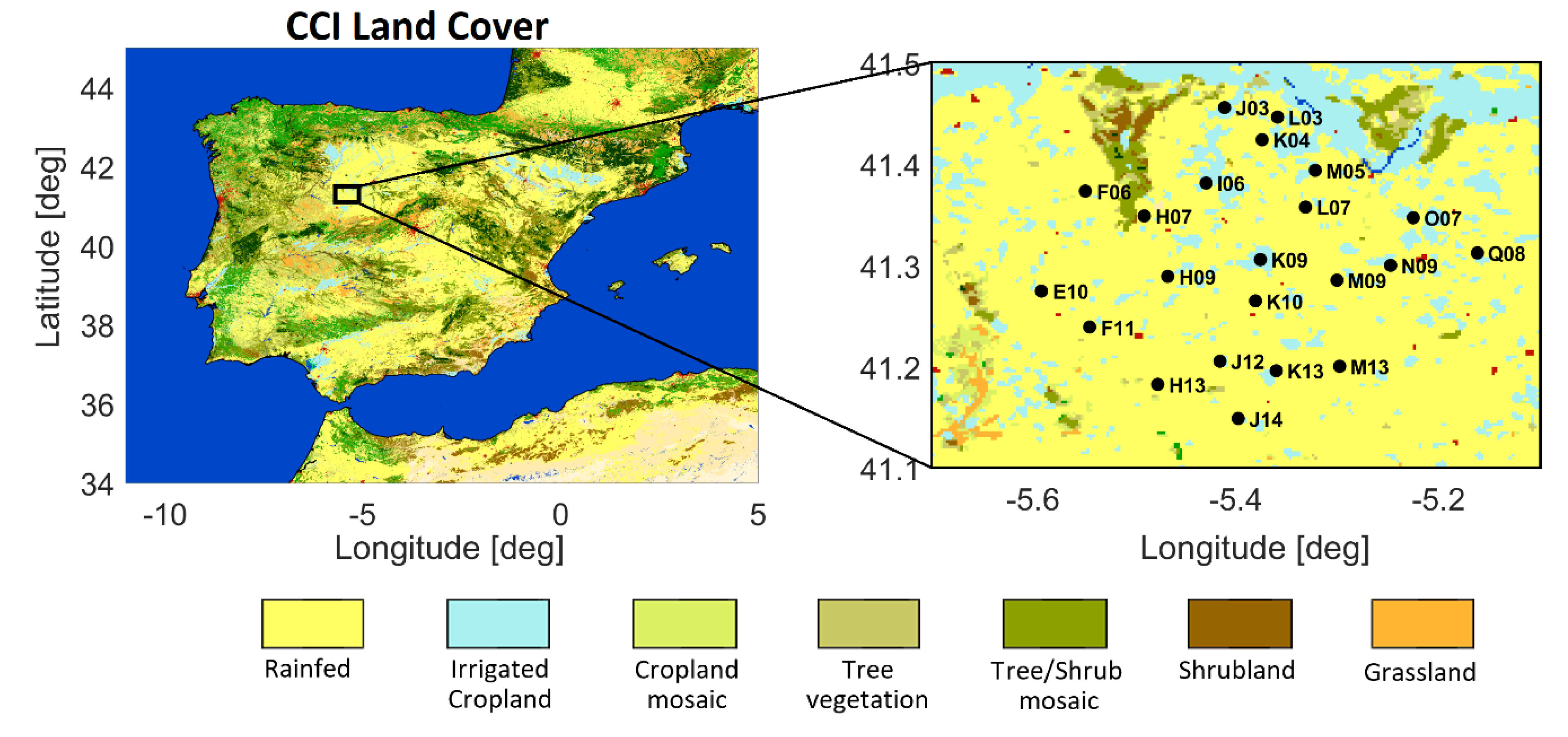
2.1.3. REMEDHUS Network

The Soil Moisture Measurements Station Network of the University of Salamanca (REMEDHUS) is an in situ network located in the central part of the Duero basin (41.1° to 41.5°N; 5.1° to 5.7°W). It contains 20 soil moisture monitoring stations that provide information at different depths (here we are using exclusively the topsoil data at 5 cm depth), and four automatic weather stations that measure precipitation, air temperature, relative humidity, wind speed, and solar radiation [36]. These stations are located within a nearly flat area of 1300 km² in a semi-arid Continental-Mediterranean agricultural region. This area receives an average annual precipitation of 385 mm, and it has a mean temperature of 12 °C [37]. Most of the region is dedicated to grow rainfed cereals, as shown in Figure 1. Other land uses within this area: irrigated crops, fallow, vineyards, or forest-pasture. The stations record the SSM data every hour, aggregated to a daily average [38] for this study.

2.2. Ancillary Data

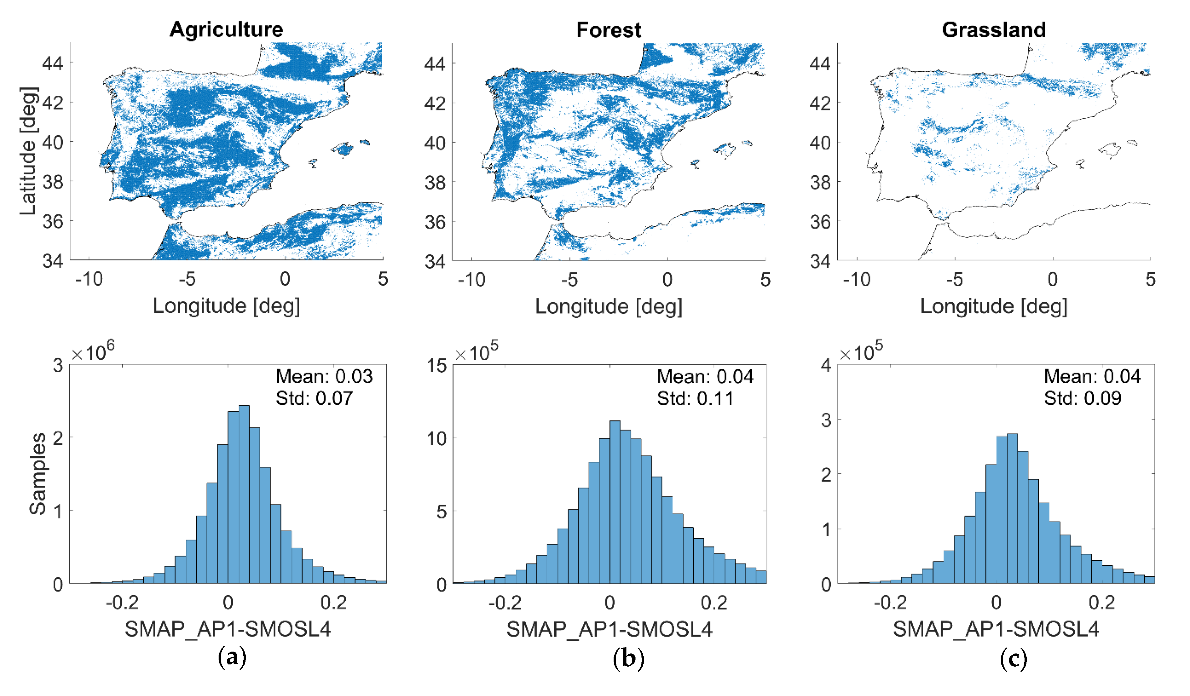
Climate Change Initiative: Land Cover

The ESA Climate Change Initiative (CCI) program includes a variety of biological, physical, and chemical variables known as ECV. Here the CCI land cover (LC) is used, which provides information of the geographical distribution of global land cover at a resolution of 300 m [39,40]. The CCI LC from year 2015 will be used in this study to characterize the dominant land cover within each SMOS/SMAP pixel. Minimal differences were observed on the CCI LC over the study region during the period 2013–2017.

3. Methodology

3.1. Statistical Analysis of SSM Time Series at the Network Scale

Ground-based SSM measurements from REMEDHUS have been selected as a benchmark for a cross-validation of the multi-scale remotely sensed SSM products. REMEDHUS stations were placed by the Water Resources Research group of the University of Salamanca (responsible for the maintenance of the network) in areas in which the land use, during the years from 2015 to 2017, were the following: fallow, rainfed, forest-pasture, vineyard and irrigated. A thorough analysis of the 20 operational in situ stations available during the study period and their comparison to satellite data was performed. For the sake of clarity and simplicity, in this work we will focus on 11 of them (see

Table 2. Land use of the region where 11 in situ stations, of the REMEDHUS network, were located, Figure 2015. 2016, and 2017 (provided by the Water Resources Research group of the University of Salamanca). The land uses are: fallow (F), rainfed (R), forest-pasture (FP), vineyard (V), irrigated (I).

	H13	H9	J3	K13	N9	O7	F11	J12	J14	K10	M9
2015	F	FP	V	I	R	R	R	R	R	R	R
2016	F	FP	V	I	R	F	F	F	F	F	F
2017	F	FP	V	I	R	R	R	R	R	R	R

). They cover the five land uses -and therefore allow studying the impact of land use on the downscaling products- and also provide a good spatial representation when averaged at the network scale.

In this first step of the analysis, we used the data provided by six stations (H13, H9, J3, K13, N9, and O7) representative of the five different land uses over the REMEDHUS network. The SMAP and the SMOS time series of the pixels overlapping these stations have been statistically evaluated with the in situ SSM at two spatial levels, at low resolution (from 9 km up to ~40 km) and at high resolution (3 km and 1 km). Performance metrics, such as the Pearson’s correlation (R), the root mean square error (RMSE), the unbiased root mean square error (uRMSE) and the bias, together with the number of available samples (N), have been computed for each station-pixel pair. These performance metrics have been calculated exactly as described in [41].

Since rainfed is the most common land cover type within the REMEDHUS area (see Figure 1), the second step of the analysis consisted in reproducing the same statistical evaluation, but using only the dataset of the stations located over rainfed/fallow land uses (F11, H13, J12, J14, K10, M9, and O7). The average value of all these rainfed/fallow stations were compared to the average of the respective SMAP and SMOS pixels covering these stations.

Additionally, statistical scores have been obtained for all seasons (DJF: December, January, February; MAM: March, April, May; JJA: June, July, August; SON: September, October, November). This analysis is needed to evaluate whether the precision (R), accuracy (bias) and quadratic errors (RMSE/uRMSE) of the studied products/methodologies have any seasonal dependence.

3.2. Analysis of the SSM Spatial Patterns

To consistently analyze the spatial features of the SMAP and SMOS SSM maps at 1 km, their maps of daily differences were computed (SMAP_AP1 minus SMOSL4) along the entire study period and the histogram of these daily SSM difference maps has been obtained, together with its mean and standard deviation (std). In addition, daily SSM difference maps have been temporally averaged and compared to the spatial distribution of the most common land cover types over the Iberian Peninsula.

Besides, taking into account different ancillary data (e.g., soil roughness, vegetation indices, skin temperature, or albedo) [24], high-resolution SMAP and SMOS SSM maps are derived from their respective T_B, as described in Section 2.1.1 and Section 2.1.2. However, there are noteworthy differences related to T_B polarizations and incidence angles. While the SMAP disaggregation methodology in (1) uses one specific polarization (vertical) with a single incidence angle (40°), the SMOS downscaling algorithm in (2) employs two polarizations (horizontal and vertical), and the average of three incidence angles (32.5° ± 5°, 42.5° ± 5°, and 52.5° ± 5°) over the same target. To analyze the influence of T_B data on the high-resolution SSM maps, the vertical SMAP L1C T_B has been compared to the vertical SMOS L1C T_B at the Earth’s surface, using exclusively the central SMOS angle (42.5°). To do so, the SMOS T_B has been corrected by the geometry of the antenna, the ionospheric and atmospheric effects, linearly interpolated to the angles range 42.5 ± 5° and binned to a 25 km EASEv2 grid. The SMAP T_B has been interpolated from the initial 36 km EASEv2 to the same grid of SMOS, using the nearest neighbor. Then, daily differences (SMAP minus SMOS T_B) have been computed from April 2015 to December 2017. The coastal areas of the Iberian Peninsula were discarded to screen out the effect of sea-land contamination.

A low- vs. high-resolution study has also been performed to assess the variations, in volumetric units, between the original and the downscaled SSM maps of the same sensor. In this way, we assessed the impact of the different downscaling methods on spatial soil moisture patterns. To do this, coarse-resolution SMAP and SMOS maps were firstly interpolated to a 1 km grid using the nearest neighbor. The comparison was done by separately calculating the daily differences between the SMAP_AP1 and the SMAPL2 maps, as well as the daily differences between SMOSL4 and SMOSL3 maps along the entire study period.

4. Results

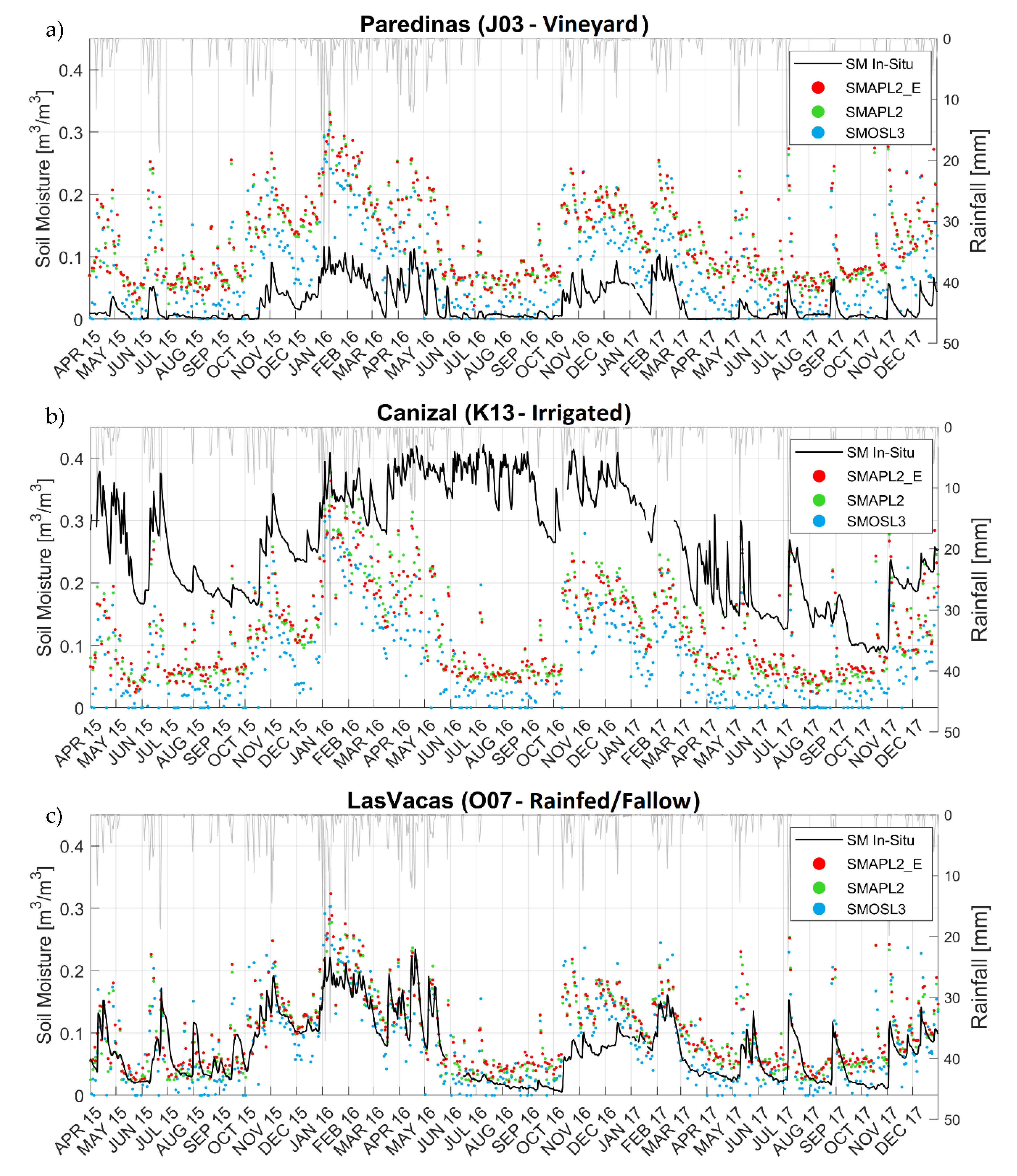
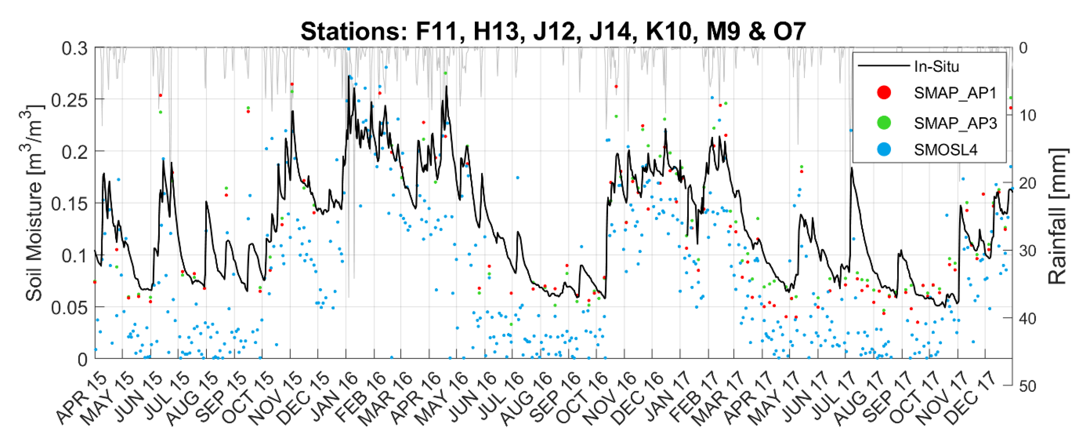
4.1. Statistical Analysis of SSM Time Series at the Network Scale

Interestingly, SMAP and SMOS satellite products agree reasonably well among them, capturing the marked wet up and dry down variations along time. Nevertheless, a strong dependence of results from comparison to in situ on land use is found. Both, SMAP and SMOS products are overestimating the in situ measurements in vineyards (Figure 2a). Instead, satellite data underestimate the in situ SSM for irrigated crops (Figure 2b), while they almost match up with in situ observations for fallow/rainfed crops (Figure 2c), which are the most common land uses in the REMEDHUS area.

The statistics derived from the temporal inter-comparison of low-resolution SSM products with in situ data using all the concurrent samples available for each dataset are summarized in

Table 3. Statistics obtained from the comparison of in situ SSM against the concurrent low-resolution (radiometer-only) pixels SSM time series: of SMAPL2_E (left), SMAPL2 (center) and SMOSL3 (right), from April 2015 to December 2017. The in situ stations used (and their respective land use) are: H13 (fallow), H9 (forest-pasture), J3 (vineyard), K13 (irrigated), N9 (rainfed) and O7 (rainfed/fallow).

	In situ vs. SMAPL2_E					In situ vs. SMAPL2					In situ vs. SMOSL3
	N [-]	R [-]	RMSE [m3m−3]	uRMSE [m3m−3]	Bias [m3m−3]	N [-]	R [-]	RMSE [m3m−3]	uRMSE [m3m−3]	Bias [m3m−3]	N [-]	R [-]	RMSE [m3m−3]	uRMSE [m3m−3]	Bias [m3m−3]
H13	540	0.83	0.052	0.044	−0.028	492	0.83	0.056	0.044	−0.035	497	0.80	0.086	0.052	−0.068
H09	524	0.64	0.136	0.075	−0.114	506	0.62	0.137	0.077	−0.113	504	0.58	0.167	0.081	−0.146
J03	550	0.85	0.115	0.046	0.106	537	0.85	0.112	0.045	0.103	516	0.73	0.075	0.048	0.057
K13	502	0.46	0.166	0.086	−0.142	483	0.48	0.167	0.086	−0.143	510	0.46	0.201	0.083	−0.183
N09	502	0.67	0.087	0.052	−0.069	536	0.65	0.076	0.055	−0.052	512	0.60	0.117	0.057	−0.102
O07	490	0.79	0.048	0.038	0.030	486	0.79	0.047	0.038	0.027	510	0.70	0.048	0.048	0.004

. Comparing the different instruments, results show that the two SMAP products have the same or a slightly higher correlation (∆R ≤ 0.12) and similar unbiased errors (∆uRMSE ≤ 0.01 m³/m³) than the SMOS product in all the study cases. There are no significant differences between the metrics obtained for the SMAP SSM (9 km vs. 36 km). Regarding the different land uses, the worst results were obtained for K13, an irrigated station, with a R (and a bias) of 0.46 (and −0.142 m³/m³) for SMAPL2_E, 0.48 (−0.143 m³/m³) for SMAPL2, and 0.46 (−0.183 m³/m³) for SMOSL3. Besides, the uRMSE of K13 is twice as high the objective accuracy of both space missions (SMOS and SMAP). This underperformance probably comes from the fact that irrigated land is not the most representative land use within the low-resolution SMAP/SMOS pixels, which is mostly covered by rainfed crops (see

Table 4. Percentage of rainfed and irrigated croplands (the two most common land covers over the REMEDHUS network) within the SMOS and SMAP pixels (36 km, 25 km, 9 km, 3 km and 1 km) enclosing the in situ stations J3 (vineyard), K13 (irrigated) and O7 (rainfed/fallow).

	J3 (Vineyard)		K13 (Irrigated)		O7 (Rainfed/Fallow)
	Rainfed (%)	Irrigated (%)	Rainfed (%)	Irrigated (%)	Rainfed (%)	Irrigated (%)
SMAPL2 (36 km)	67.81	20.83	80.27	17.26	67.97	24.68
SMOSL3 (25 km)	61.06	30.51	92.54	6.47	61.06	30.51
SMAPL2_E (9 km)	39.71	52.16	93.08	6.66	68.69	23.27
SMAP_AP3 (3 km)	43.80	42.98	79.55	20.45	66.94	33.06
SMOSL4 (1 km)	56.25	43.75	68.75	31.25	75.00	25.00

). On the contrary, the best results are obtained for the stations located over rainfed/fallow land cover (H13 and O07), with a R between 0.79 and 0.83 for both SMAP products (SMAPL2_E and SMAPL2), and between 0.70 and 0.80 for SMOS. Their bias is low, between 0.027 and 0.035 m³/m³ for SMAP, and between 0.004 and 0.068 m³/m³ for SMOS, in absolute values. The uRMSE of these two stations are around 0.04–0.05 m³/m³, meeting or almost meeting required accuracy of both missions. In the case of vineyards (J03), intermediate results are obtained. The highest R is obtained for two SMAP products (0.85), but a high R is also obtained for SMOSL3 (0.73). The uRMSE is very similar (from 0.045 to 0.048 m³/m³). However, the bias of J03 is similar for SMOSL3 (0.057 m³/m³), but the SMAP ones are up to two or three times higher (0.106 and 0.103 m³/m³) than the aforementioned ones for rainfed/fallow. At these spatial scales, the number of available samples of SMAP and SMOS with in situ samples are of the same order (around 500 days), ensuring a robust statistical analysis.

When analyzing the metrics derived from the validation of SMAP and SMOS at high resolution (see

Table 5. Statistics obtained from the comparison of in situ SSM against the concurrent high-resolution pixels SSM time series: of SMAP_AP1 at 1 km (left), SMAP_AP3 at 3 km (center) and SMOSL4 at 1 km (right), from April 2015 to December 2017. The in situ stations used (and their respective land use) are: H13 (fallow), H9 (forest-pasture), J3 (vineyard), K13 (irrigated), N9 (rainfed) and O7 (rainfed/fallow).

	In Situ vs. SMAP_AP1					In Situ vs. SMAP_AP3					In Situ vs. SMOSL4
	N [-]	R [-]	RMSE [m3m−3]	uRMSE [m3m−3]	Bias [m3m−3]	N [-]	R [-]	RMSE [m3m−3]	uRMSE [m3m−3]	Bias [m3m−3]	N [-]	R [-]	RMSE [m3m−3]	uRMSE [m3m−3]	Bias [m3m−3]
H13	100	0.81	0.062	0.040	−0.048	100	0.86	0.046	0.038	−0.025	489	0.80	0.089	0.045	−0.076
H09	96	0.56	0.164	0.086	−0.139	96	0.60	0.155	0.084	−0.131	443	0.59	0.175	0.079	−0.156
J03	98	0.70	0.093	0.046	0.081	98	0.83	0.121	0.043	0.114	513	0.72	0.085	0.054	0.066
K13	97	0.45	0.172	0.097	−0.142	97	0.51	0.156	0.088	−0.129	493	0.42	0.205	0.085	−0.186
N09	101	0.45	0.120	0.071	−0.097	101	0.57	0.101	0.058	−0.082	503	0.63	0.119	0.056	−0.105
O07	98	0.66	0.076	0.063	0.042	99	0.78	0.076	0.050	0.056	501	0.71	0.047	0.047	−0.001

), the irrigated station K13 keeps showing the worst results as in the low-resolution case: a R (and a bias) of 0.45 (−0.142 m³/m³) for SMAP_AP1, 0.51 (−0.129 m³/m³) for SMAP_AP3, and 0.42 (−0.186 m³/m³) for SMOSL4. This indicates that irrigated areas are not even spatially representative at the scales of 3 km to 1 km, which denotes the small extent of these areas within the satellite footprint (see Table 4).

Similarly, the best results are obtained for the stations H13 and O07, with R between 0.66 and 0.86 for SMAP_AP1 and SMAP_AP3, and between 0.71 and 0.80 for SMOSL4. The lowest bias is precisely observed in H13 and O07, ranging between 0.025 and 0.056 m³/m³ for SMAP, and from 0.001 to 0.076 m³/m³ for SMOS, in absolute values. Again, the reason for that is the predominance of rainfed crops and fallow regions over REMEDHUS (see Table 4). Therefore, both satellites mostly see the land cover types leading to a cover-characteristic signal at low- as well as at high-resolution. As previously observed in Table 3, the metrics for vineyard are in a well acceptable range. On the one hand, taking into account both SMAP and SMOS, R varies between 0.70 and 0.83, and the uRMSE is always around 0.04–0.05 m³/m³. On the other hand, the bias of J03 is doubled or even tripled (0.081 and 0.114 m³/m³) with respect to the stations H13 and O07. All the SMAP and SMOS products are overestimating the in situ measurements of J03. One reason could be that grapevines are settled on very fine sand, which causes the water not to be retained and it quickly percolates into deeper layers. Additionally, the vineyard areas of REMEDHUS are not spatially representative at scales of 1 km and beyond.

Due to the missing synchronization of SMAP and Sentinel-1 acquisition orbits, the number of samples is much lower in the SMAP_AP1 and SMAP_AP3 (96 to 101 days) than in the SMOSL4 time series (443 to 513).

Similar statistical scores are obtained for the SMOS products when the same number of samples is used at high and low resolution, in line with the results obtained in a previous study [13]. When the same analysis is conducted for the SMAP products, only slightly worst performances are obtained for the SMAP_AP1 product.

Table 6. Statistics obtained from the comparison of in situ SSM against the high-resolution pixel SSM of SMAP_AP1 at 1 km (left), SMAP_AP3 at 3 km (center) and SMOSL4 at 1 km (right) from April 2015 to December 2017 for the different seasons of the year and also for the entire study period (ESP). Statistics are obtained after averaging all-time series of rainfed/fallow stations (F11, H13, J12, J14, K10, M9 and O7) and the pixels that contain these stations.

	In situ vs. SMAP_AP1					In situ vs. SMAP_AP3					In situ vs. SMOSL4
	N [-]	R [-]	RMSE [m3m−3]	uRMSE [m3m−3]	Bias [m3m−3]	N [-]	R [-]	RMSE [m3m−3]	uRMSE [m3m−3]	Bias [m3m−3]	N [-]	R [-]	RMSE [m3m−3]	uRMSE [m3m−3]	Bias [m3m−3]
DJF	17	0.87	0.056	0.053	0.018	17	0.92	0.060	0.048	0.035	88	0.87	0.056	0.047	−0.031
MAM	22	0.91	0.037	0.033	−0.017	22	0.90	0.027	0.026	−0.008	119	0.72	0.071	0.041	−0.058
JJA	26	0.62	0.037	0.035	−0.012	27	0.64	0.035	0.035	−0.006	128	0.65	0.073	0.030	−0.067
SON	33	0.85	0.034	0.033	0.008	33	0.86	0.034	0.032	0.011	125	0.78	0.052	0.041	−0.032
ESP	98	0.86	0.040	0.040	−0.002	99	0.87	0.039	0.038	0.006	460	0.82	0.064	0.043	−0.048

shows the statistics obtained between the average SSM values of the stations located over a rainfed/fallow land use (F11, H13, J12, J14, K10, M9, and O7) and the average of the concurrent SMAP and SMOS products at high-resolution (see Figure 3). Lower correlations are obtained during summer season (0.62, 0.64 and 0.65, for SMAP_AP1, SMAP_AP3 and SMOSL4, respectively). This is consistent with the results of previous studies [13]. Slightly better results are obtained for SMAP in terms of R (and bias) 0.88 (0.014 m³/m³), against SMOS, 0.79 (0.04 m³/m³) calculated as an average of DJF, MAM, and SON.

4.2. Analysis of the SSM Spatial Patterns

The study carried out in the previous section shows a general agreement between the temporal dynamics of all the considered SSM products regardless of their spatial resolution (low resolution: ~40 km, 9 km vs. high resolution: 3 km, 1 km). However, as it can be seen from the maps shown in Figure 4, there are clearly visible differences in the spatial patterns attained by the downscaled SMAP and SMOS high-resolution products. In this section, we examine these differences and conduct specific analyses to test two hypothesis: (i) that they are due to differences in the multi-sensor synergies they are built upon (optical-microwave or active-passive) and (ii) that they are due to the rationale of the approach (e.g., whether the downscaling is conducted in brightness temperature- or in the soil moisture-space).

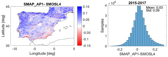
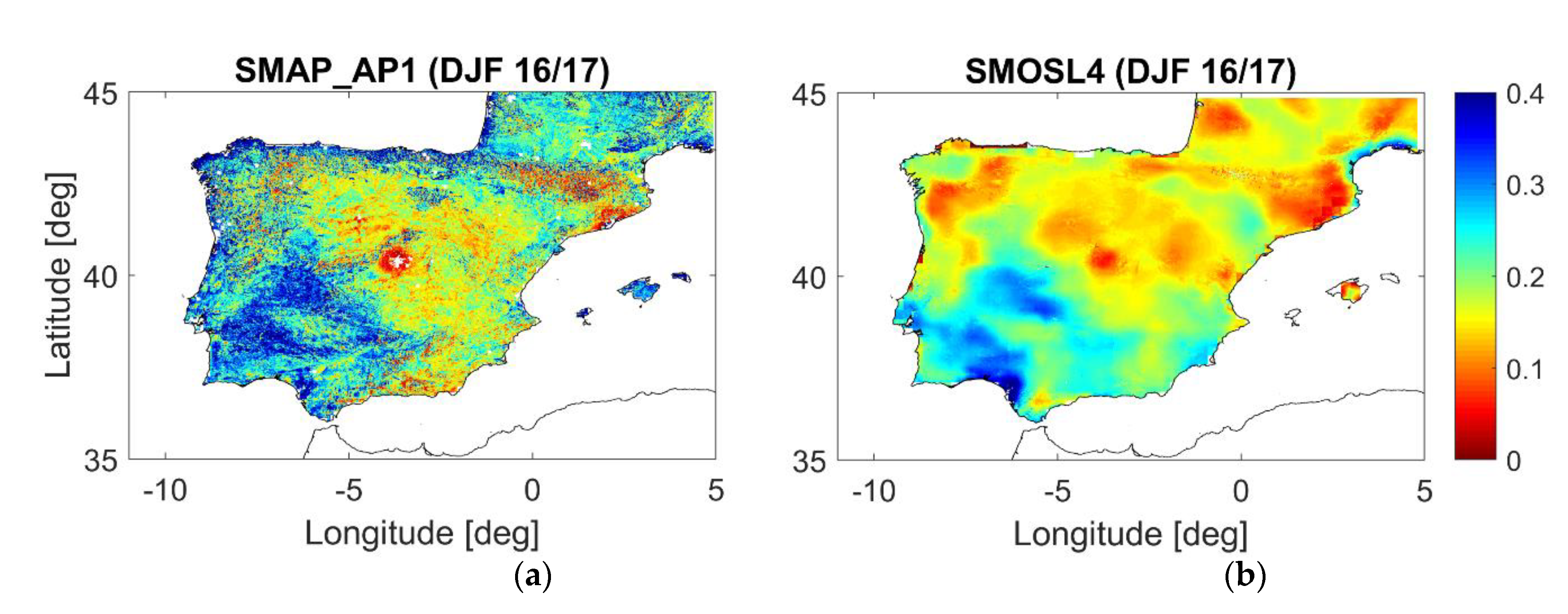
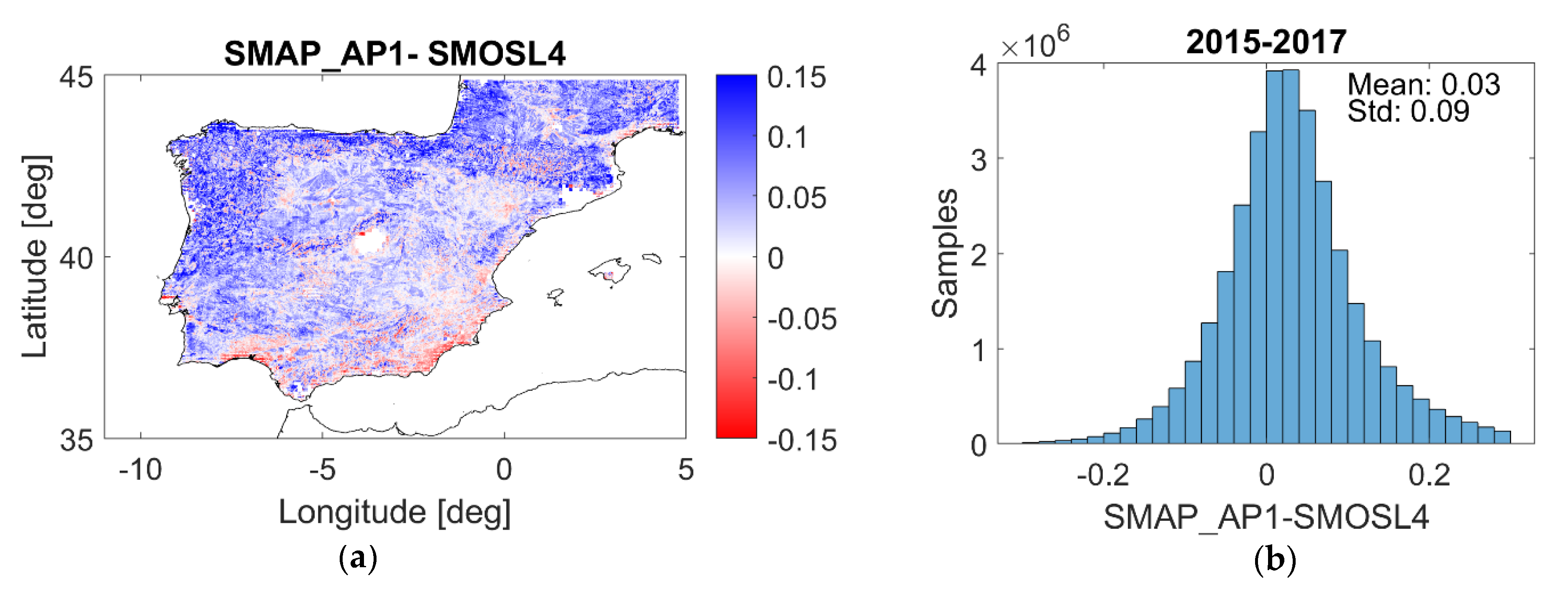
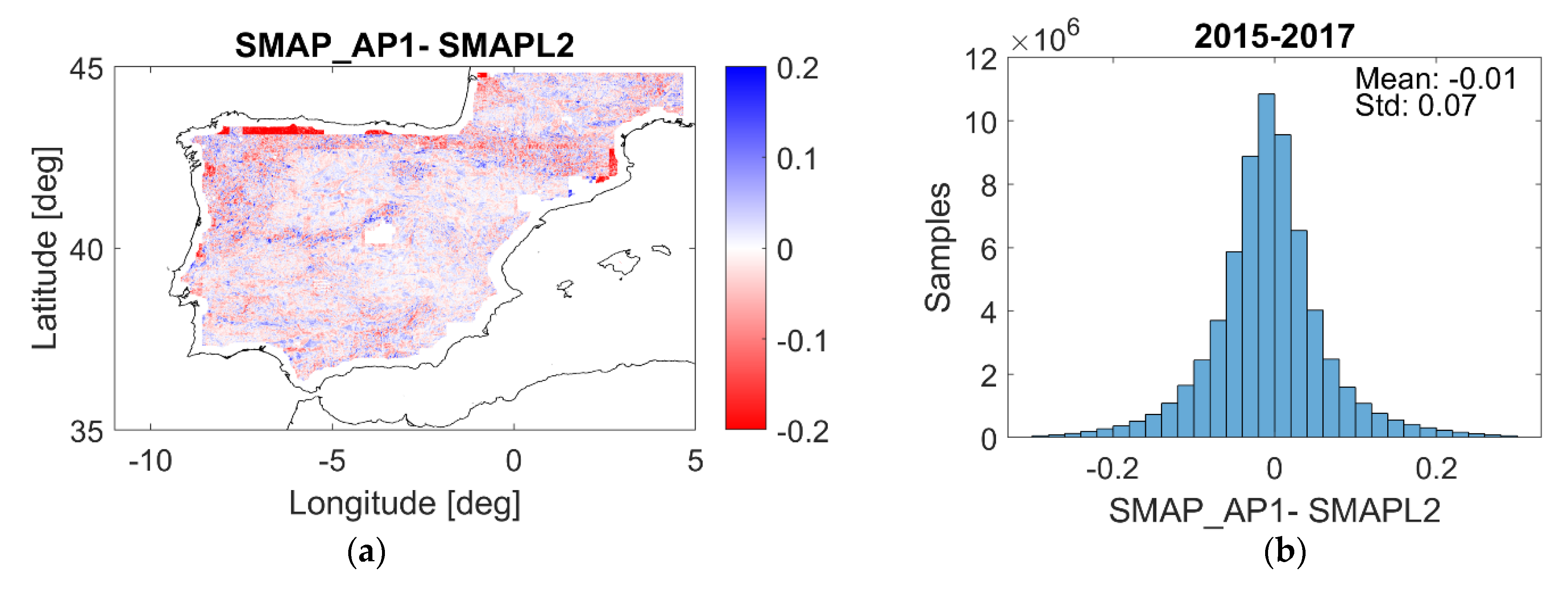
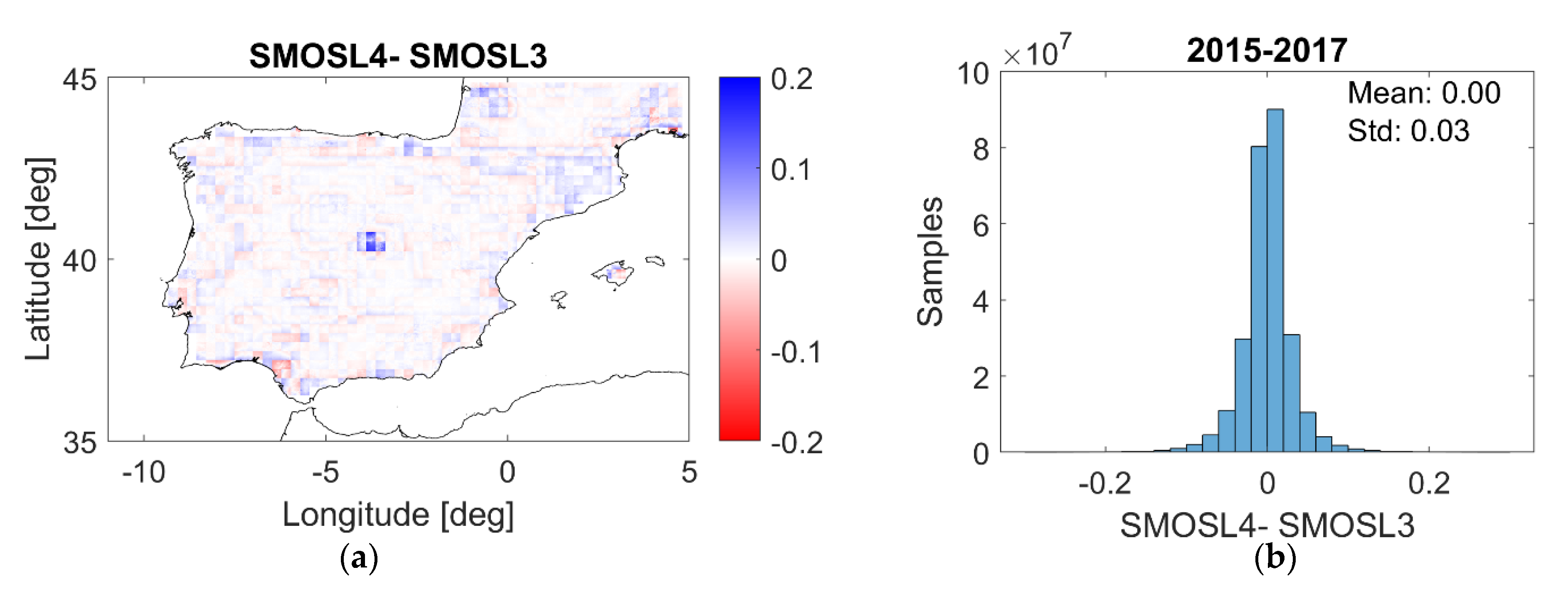
4.2.1. Comparison of SSM Enhanced Resolution Products

Figure 5 shows the daily differences (map and histogram) between the SMAP and SMOS products at 1 km (SMAP_AP1 minus SMOSL4) for the whole study period. The mean of these differences is minimal (of 0.03 m³/m³), less than their target accuracy, and their std is also low (of 0.09 m³/m³). The same behavior is observed when this study is performed on a year-to-year basis (not shown). In addition, we conducted the same analysis per season, and we obtained that daily differences ranged between 0.03 and 0.04 m³/m³ in mean and from 0.05 to 0.07 m³/m³ in std (not shown). These results affirm that the differences cannot be explained by seasonal or yearly differences (e.g., dry or wet year). Yet the temporally-averaged map of daily SSM differences (Figure 5a) reveals that there is a geographic spatial pattern that persists over time when comparing the two high-resolution products, with higher differences located in the north, northwest and west of the Iberian Peninsula, in close correspondence to forested areas (see land cover maps on Figure 6).

The possible dependence of the differences between the two downscaled products on the land cover was further examined. Pixels from the temporally-average map of SSM differences (Figure 5a) were grouped for the most common land cover classes (agriculture, forest and grassland) and their histograms were analyzed (see Figure 6). In general, pixels with SSM differences (SMAP minus SMOS) equal or above 0.1 m³/m³ are located within forests (66.71% of the pixels) or agriculture (22.47% of the pixels). The largest SSM differences are observed for forest land cover, with a mean of 0.04 m³/m³ and a std of 0.11 m³/m³.

Land cover only partially explains the SSM differences between the SMAP and SMOS products at 1 km. Results show that soil moisture values provided by SMAP over the Iberian Peninsula are systematically higher than the ones provided by SMOS (see Figure 5), although the absolute difference is minimal (mean difference of 0.03 m³/m³). The SSM values of SMOS exceed those of SMAP less often and with lower intensity, but this effect is mostly occurring in coastal areas. The same SSM difference pattern is found in the temporally-averaged map of daily T_B differences (SMAP minus SMOS T_B) shown on Figure 7. Since the spatial pattern is already present at T_B level, we can conclude it was not introduced by neither SMAP nor SMOS downscaling methodologies. Figure 7b shows the histogram of the daily T_B differences, with an absolute mean value of 2.92 K. In order to understand to what extent, the 2.92 K cold bias could affect SMAP or SMOS SM retrievals, we analyzed Davenport et al. in [42], who conducted a sensitivity analysis of soil moisture retrieval using the applied tau-omega microwave emission model. A bias of about 3° (K) T_B approximately corresponds to 3–4 (vol.%) error in estimating volumetric soil water content, which would fit to the bias ranges reported in our study.

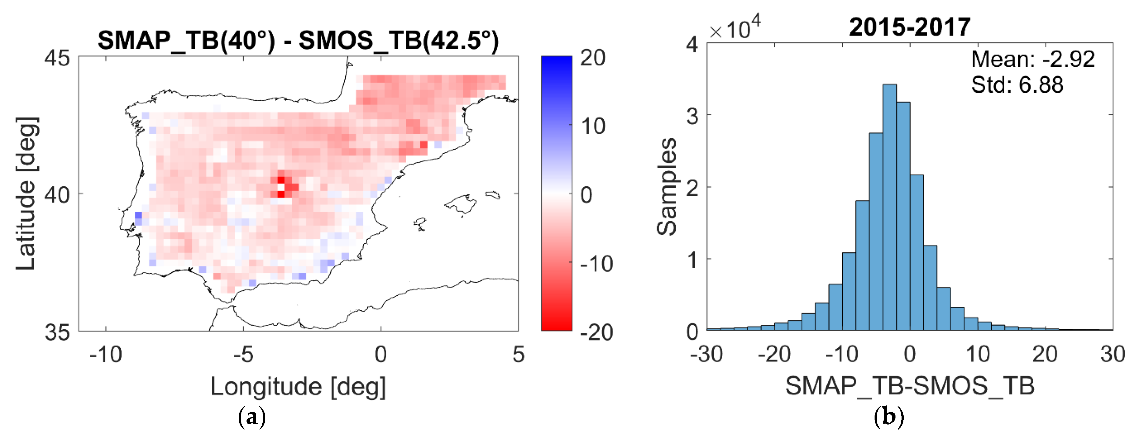
4.2.2. Downscaling Impact on SSM Differences

Figure 8 and Figure 9 show the maps and histograms of daily SSM differences between SMAP_AP1 and SMAPL2 (1 km vs. 36 km), and between SMOSL4 and SMOSL3 (1 km vs. 25 km), respectively. The mean (and std) obtained after calculating the differences along the complete study period are −0.01 m³/m³ (0.07 m³/m³) for SMAP, and of ~0 m³/m³ (0.03 m³/m³) for SMOS. Although mean differences are minimal over the whole domain for both sensors, the resulting average map of the SMAP SSM differences reveal some underlying spatial patterns. The highest positive differences obtained for SMAP are concentrated in the forested regions (see Figure 6) and the highest negative differences appear near the coast and in areas of complex topography. This is possibly due to the reduced sensitivity of the Sentinel 1 signal at C-band to soil moisture in presence of significant vegetation backscattering. According to [12], this leads to a decrease in T_B after downscaling and therefore to an increase in estimated soil moisture. Also, the temporally-averaged map of SMOS SSM differences exhibits an underlying boxing effect that can be explained by the use of SMOS SSM at low-resolution as a reference to obtain the downscaling parameters of (2), as previously observed in [13,21]. However, this effect is nonetheless negligible and does not have a significant impact in the enhanced resolution product.

5. Discussion

Validation and comparison of SSM satellite products using in situ networks data is a difficult task. Many confounding factors can intervene and must be taken into account when interpreting the obtained results. Importantly for this work, it is essential to understand that the representativeness of each satellite dataset plays a crucial role when validated. In the case of the SMAP and SMOS products presented in this study, the data is stored in maps with spatial grid cells of 36, 25, 9, 3, or 1 km. The information contained in these cells represents an areal-averaged value, while the in situ measurements represent an isolated data point. Measurements of the most representative (in terms of land cover within satellite cells) SSM in situ stations have been averaged (as can be seen in Figure 3 and Table 6) to validate the large scale SSM estimates provided by the satellites [37,43]. It is found that validating satellite-based estimates works best with in situ measurements in locations where the dominant land cover of the satellite footprint prevails.

Besides the representativeness error due to the comparison of point-scale vs. areal-averaged measurements, the mismatch between satellite observations and in situ measurements can also be originated by the penetration depth of microwave frequencies at L-band, which is of 5 cm on average but also depends on the soil moisture content itself (with greater penetration on drier soils) [3]. In contrast, measurements of the REMEDHUS network probes are placed at a depth of 5 cm. This could be one of the reasons explaining the low correlations obtained under water-limited conditions (see Table 6 for JJA), when the soil surface dries out and therefore in situ sensors might measure slightly wetter values than satellites. Moreover, the surface temperature used in SMAP and SMOS retrievals is derived from models. While the SMAP surface temperature is derived from the NASA GEOS-5 model, the SMOS surface temperature is obtained from the ECMWF model. An underestimation of the surface temperature leads to an overestimation of the soil emissivity and, as a result, to an underestimation of the SSM. This could explain the dry bias shown by the SMAP and the SMOS products with respect to the most representative in situ stations in REMEDHUS. Our results are in line with previous studies which have also reported this dry bias when comparing the SSM SMOS products (at high and low-resolution) against the in situ data provided by VAS (Spain), SMOSMANIA (France), and OzNet (Australia) networks [13,21,44]. In Figure 2 SMOS soil moisture estimates with a very low value close to zero can be found, mostly during the summer periods. These values have not been filtered in this study, as the product quality flags do not report they are measurement errors. However, we conducted specific tests and confirmed that they do not affect our overall conclusions (not shown).

Some differences between the SMAP and the SMOS products are intrinsic to the instrument they carry; while SMOS uses an interferometric radiometer with 69 receivers distributed on an Y-shaped antenna array and measurements at different incidence angles are obtained in each snapshot, SMAP uses a large rotating antenna and measurements are performed at a constant incidence angle of 40°. On the other hand, the SSM retrieval algorithms have been tailored to the SMAP and SMOS instrument characteristics, and they involve the use of dedicated techniques to reduce or correct disturbing factors (e.g., surface roughness, soil temperature and vegetation canopy). In a global study conducted by Mariko et al. [45] the SMAP SSM was compared against the one provided by SMOS, Aquarius, Advanced Scatterometer (ASCAT) and Advanced Microwave Scanning Radiometer 2 (AMSR2). Overall, they found that SMAP and SMOS appeared to be the most similar among the five SSM products, in terms of uRMSE and R, excluding forested areas where some discrepancies were found, with SMOS being generally slightly wetter than SMAP. For the particular case of the Iberian Peninsula, which is mostly covered by crops and forested areas, we showed that SMAP is generally wetter than SMOS. Although differences are minor, we showed they are already present at the T_B level (see Figure 7), and are also translated to the SMOS and SMAP derived products at enhanced spatial resolutions (see Figure 5). Mariko et al. [45], indicate that a highly potential cause of the mismatch between the SMAP and the SMOS products is the use of different ancillary data in the retrieval algorithm. Although both algorithms are based on the tau-omega model they use different land cover maps to select the albedo, roughness coefficient and the vegetation opacity; SMAP uses the International Geosphere Biosphere Program (IGBP) [46], and SMOS uses the ECOCLIMAP [47]. This could explain the differences observed between the original SMAP and the SMOS products (~40 km), but also between the satellite observations and the in situ measurements along the whole study.

Focusing on the enhanced resolution SSM products, they allow us to develop applications that will otherwise not be possible using exclusively SMAP and SMOS products in their original resolutions (~40 km). However, we showed that even the higher resolutions (3 and 1 km) of SSM maps may not be completely suitable for local or regional applications if the study area is small and the land cover is not representative of the SMAP or SMOS pixel to which it belongs (Figure 2a,b). In [48], Merlin et al. proposed a performance metric for soil moisture downscaling methods and it was applied to the 1 km disaggregation based on physical and theoretical scale change (DISPATCH) data in central Morocco. They showed that disaggregation applied to irrigated areas surrounded by drylands reduced the negative bias in SMOS observations at 1 km with respect to in situ data, but was not yet fully able to solve the sub-pixels variability in soil moisture. The scientific contribution of the downscaled SMAP and SMOS products is undeniable, adding value in a wide range of applications, such as the prevention management of insect pests [6], the prevention of forest fires [7,8] and the early detection of wild fires [9], but further improvements are needed to reduce the uncertainties when merging information from different sensors.

6. Summary and Conclusions

In this study, several space-borne SSM products (SMAP and SMOS), and their derived products at enhanced spatial resolution (SMAP/Sentinel-1 and SMOS/ERA5/MODIS) have been compared in space, and time.

For the temporal comparison, the in situ information of the REMEDHUS network has been used as a benchmark. In order to study the behavior of the remotely sensed data in different scenarios, we selected a variety of in situ SSM stations located in areas with different land uses (fallow, forest-pasture, vineyard, irrigated, and rainfed). We showed that, independently of the spatial resolution, all the SSM products were able to capture significant rainfall events (e.g., the rainfall event occurring in January 2016, see Figure 2), and seasonality pattern (summers with low and winters with high soil moisture values, see Figure 2 and Figure 3). However, even the highest-resolution product used in this study (1 km) is not fine enough to capture local differences which are not dominant at the pixel scale, like the small irrigated areas where station K13 is located (see Table 3 and Table 5). Consequently, when comparing the remotely sensed data with REMEDHUS measurements it is crucial to understand the representativeness of one in situ station within the satellite footprint. In situ SSM measurements are representative at the point scale and are highly sensitive to both the soil characteristics and the effects of precipitation. There are multiple strategies to upscale in situ soil moisture measurements for comparison with satellite-based estimates [49,50]. In this study, we have decided to average the SSM values of the most representative (in terms of prevailing land cover) in situ stations within the satellite footprint. One of the best results when comparing low-resolution as well as high-resolution SMAP/SMOS-based estimates against the in situ measurements, are obtained for the stations H13 and O07, which are located in regions with rainfed or fallow land use (the most common land uses in REMEDHUS). On the contrary, the worst results were obtained over stations J3 (vineyard) and K13 (irrigated), which represent only a minor land cover fraction within the footprints (see Table 4).

Statistically, the differences between the SMAP and SMOS products are considerably low, e.g., at low-resolution, for the station H13 the correlation (and the unbiased error) are 0.83 (0.044 m³/m³) for SMAP (SMAPL2_E), 0.8 (0.052 m³/m³) for SMOS (SMOSL3); at high-resolution these statistics are 0.81 (0.04 m³/m³) for SMAP, and 0.8 (0.045 m³/m³) for SMOS. From Figure 3 and Table 6 it can be seen that both SMOS and SMAP have a slightly worst performance in terms of correlation (~0.6) during the summer season. In addition, SMOS shows an important bias (−0.067 m³/m³) in this period.

Concerning the spatial analysis, the high-resolution (downscaled) SMAP (passive/active) and SMOS (passive/optical) products have been compared across the Iberian Peninsula. Overall, SMAP is slightly wetter than SMOS, especially in the north, northwest, and west of the Iberian Peninsula. These differences are more pronounced over forested areas, which may be due to the fact that the microwave (radar) signal at C-band used in the SMAP product is not able to penetrate through dense (forested) vegetation [12,51]. Moreover, the differences between the two products can also be seen at the brightness temperature level and therefore are not introduced by the downscaling methodology.

This satellite inter-comparison study has provided and confirmed insights into the SMOS and SMAP multi-scale SSM products that are currently operational. These products are required in a wide spectrum of application and research studies, generally at the best radiometric accuracy and spatial resolution possible. Over the Iberian Peninsula, we showed that all products generally agree in their temporal dynamics, with lowest performances in summer, and SMAP-derived products being wetter than SMOS ones. Yet some differences in spatial patterns are observed in the high-resolution products, linked to the fine-scale information they use and the multi-sensor synergies employed, especially in forested areas. In future studies, the presented analysis can be extended to other regions of the world that have a sufficiently dense soil moisture network to establish reliable estimates at multi-scale resolutions. Also, the proposed spatio-temporal analyses can be widened to global scales with the use of sparse in situ networks.

References

1. Lahoz, W.; Blyverket, J.; Hamer, P. Product Validation and Intercomparison Report (PVIR) Revision 3 2018. Available online: https://www.esa-soilmoisture-cci.org/sites/default/files/documents/ESA_CCI_Soil_Moisture_D4.1.2_PVIR_Revision3_v2.6.pdf (accessed on 20 December 2019).
2. Entekhabi, D.; Njoku, E.G.; O’Neill, P.E.; Kellogg, K.H.; Crow, W.T.; Edelstein, W.N.; Entin, J.K.; Goodman, S.D.; Jackson, T.J.; Johnson, J.; et al. The Soil Moisture Active Passive (SMAP) Mission. Proc. IEEE 2010, 98, 704–716. [Google Scholar] [CrossRef]
3. Ulaby, F.; Long, D. Microwave Radar and Radiometric Remote Sensing; University of Michigan Library: Lansing, MI, USA, 2014. [Google Scholar]
4. Konings, A.G.; Piles, M.; Das, N.; Entekhabi, D. L-band vegetation optical depth and effective scattering albedo estimation from SMAP. Remote Sens. Environ. 2017, 198, 460–470. [Google Scholar] [CrossRef]
5. Jackson, T.; Schmugge, T. Vegetation effects on the microwave emission of soils. Remote Sens. Environ. 1991, 36, 203–212. [Google Scholar] [CrossRef]
6. Escorihuela, M.J.; Merlin, O.; Stefan, V.; Moyano, G.; Eweys, O.A.; Zribi, M.; Kamara, S.; Benahi, A.S.; Ebbe, M.A.B.; Chihrane, J.; et al. SMOS based high resolution soil moisture estimates for desert locust preventive management. Remote Sens. Appl. Soc. Environ. 2018, 11, 140–150. [Google Scholar]
7. Chaparro, D. Surface moisture and temperature trends anticipate drought conditions linked to wildfire activity in the Iberian Peninsula. Eur. J. Remote Sens. 2016, 49, 955–971. [Google Scholar] [CrossRef] [Green Version]
8. Chaparro, D.; Vall-Llossera, M.; Piles, M.; Camps, A.; Rüdiger, C.; Riera-Tatché, R. Predicting the Extent of Wildfires Using Remotely Sensed Soil Moisture and Temperature Trends. IEEE J. Sel. Top. Appl. Earth Obs. Remote Sens. 2016, 9, 2818–2829. [Google Scholar] [CrossRef] [Green Version]
9. Chaparro, D.; Vayreda, J.; Vall-Llossera, M.; Banque, M.; Piles, M.; Camps, A.; Martinez-Vilalta, J. The Role of Climatic Anomalies and Soil Moisture in the Decline of Drought-Prone Forests. IEEE J. Sel. Top. Appl. Earth Obs. Remote Sens. 2017, 10, 503–514. [Google Scholar] [CrossRef]
10. Sabaghy, S.; Walker, J.P.; Renzullo, L.J.; Jackson, T.J. Spatially enhanced passive microwave derived soil moisture: Capabilities and opportunities. Remote Sens. Environ. 2018, 209, 551–580. [Google Scholar] [CrossRef]
11. Peng, J.; Loew, A.; Merlin, O.; Verhoest, N.E.C. A review of spatial downscaling of satellite remotely sensed soil moisture. Rev. Geophys. 2017, 55, 341–366. [Google Scholar] [CrossRef]
12. Jagdhuber, T.; Baur, M.; Akbar, R.; Das, N.N.; Link, M.; He, L.; Entekhabi, D. Estimation of active-passive microwave covariation using SMAP and Sentinel-1 data. Remote Sens. Environ. 2019, 225, 458–468. [Google Scholar] [CrossRef]
13. Portal, G.; Vall-Llossera, M.; Piles, M.; Camps, A.; Chaparro, D.; Pablos, M.; Rossato, L. A Spatially Consistent Downscaling Approach for SMOS Using an Adaptive Moving Window. IEEE J. Sel. Top. Appl. Earth Obs. Remote Sens. 2018, 11, 1883–1894. [Google Scholar] [CrossRef]
14. Portal, G.; Vall-Llosscra, M.; Piles, M.; Camps, A.; Chaparro, D.; Pablos, M.; Rossato, L.; Aabouch, K. Microwave and Optical Data Fusion for Global Mapping of Soil Moisture at High Resolution. IGARSS 2018 IEEE Int. Geosci. Remote Sens. Symp. 2018, 11, 341–344. [Google Scholar]
15. Piles, M.; Entekhabi, D.; Camps, A. A Change Detection Algorithm for Retrieving High-Resolution Soil Moisture From SMAP Radar and Radiometer Observations. IEEE Trans. Geosci. Remote Sens. 2009, 47, 4125–4131. [Google Scholar] [CrossRef]
16. Jagdhuber, T.; Konings, A.G.; McColl, K.A.; Alemohammad, S.H.; Das, N.N.; Montzka, C.; Link, M.; Akbar, R.; Entekhabi, D. Physics-Based Modeling of Active and Passive Microwave Covariations Over Vegetated Surfaces. IEEE Trans. Geosci. Remote Sens. 2019, 57, 788–802. [Google Scholar] [CrossRef]
17. Piles, M.; McColl, K.A.; Entekhabi, D.; Das, N.; Pablos, M. Sensitivity of Aquarius Active and Passive Measurements Temporal Covariability to Land Surface Characteristics. IEEE Trans. Geosci. Remote Sens. 2015, 53, 1–12. [Google Scholar] [CrossRef] [Green Version]
18. Das, N.N.; Entekhabi, D.; Dunbar, R.S.; Chaubell, M.J.; Colliander, A.; Yueh, S.; Jagdhuber, T.; Chen, F.; Crow, W.; O’Neill, P.E.; et al. The SMAP and Copernicus Sentinel 1A/B microwave active-passive high resolution surface soil moisture product. Remote Sens. Environ. 2019, 233, 111380. [Google Scholar] [CrossRef]
19. Carlson, T.N.; Gillies, R.R.; Perry, E.M. A method to make use of thermal infrared temperature and NDVI measurements to infer surface soil water content and fractional vegetation cover. Remote Sens. Rev. 1994, 9, 161–173. [Google Scholar] [CrossRef]
20. Piles, M.; Sánchez, N.; Vall-Llossera, M.; Camps, A.; Martínez-Fernández, J.; Martínez, J.; Gonzalez-Gambau, V. A Downscaling Approach for SMOS Land Observations: Evaluation of High-Resolution Soil Moisture Maps Over the Iberian Peninsula. IEEE J. Sel. Top. Appl. Earth Obs. Remote Sens. 2014, 7, 3845–3857. [Google Scholar] [CrossRef] [Green Version]
21. Piles, M.; Petropoulos, G.P.; Sánchez, N.; González-Zamora, Á.; Ireland, G. Towards improved spatio-temporal resolution soil moisture retrievals from the synergy of SMOS and MSG SEVIRI spaceborne observations. Remote Sens. Environ. 2016, 180, 403–417. [Google Scholar] [CrossRef] [Green Version]
22. Pablos, M.; Piles, M.; González-Haro, C. BEC SMOS Land Products Description. 2019. Available online: http://bec.icm.csic.es/doc/BEC-SMOS-0002-PD-Land.pdf (accessed on 20 December 2019).
23. Entekhabi, D.; Yueh, S.; O’Neill, P.E.; Kellogg, K.H.; Allen, A.; Bindlish, R.; Brown, M.; Chan, S.; Colliander, A.; Crow, W.T.; et al. SMAP Handbook Soil Moisture Active Passive Mapping Soil Moisture and Freeze/Thaw from Space; National Aeronautics and Space Administration: Pasadena, CA, USA, 2014.
24. SMAP L2 Radiometer Half-Orbit 36 km EASE-Grid Soil Moisture, Version 6|National Snow and Ice Data Center. Available online: https://nsidc.org/data/SPL2SMP/versions/6 (accessed on 13 October 2019).
25. SMAP Enhanced L2 Radiometer Half-Orbit 9 km EASE-Grid Soil Moisture, Version 3|National Snow and Ice Data Center. Available online: https://nsidc.org/data/SPL2SMP_E/versions/3 (accessed on 13 October 2019).
26. SMAP/Sentinel-1 L2 Radiometer/Radar 30-Second Scene 3 km EASE-Grid Soil Moisture, Version 2|National Snow and Ice Data Center. Available online: https://nsidc.org/data/SPL2SMAP_S/versions/2 (accessed on 13 October 2019).
27. Chan, S. Level 2 Passive Soil Moisture Product Specification Document. 2019. Available online: https://nsidc.org/sites/nsidc.org/files/technical-references/D72547%20SMAP%20L2_SM_P%20PSD%20Version%205.1.pdf (accessed on 20 December 2019).
28. Chan, S.; Njoku, E.; Colliander, A. Algorithm Theoretical Basis Document Level 1C Radiometer Data Product; 2014. Available online: https://smap.jpl.nasa.gov/system/internal_resources/details/original/279_L1C_TB_ATBD_RevA_web.pdf (accessed on 20 December 2019).
29. El Hajj, M.; Baghdadi, N.; Zribi, M.; Rodriguez-Fernandez, N.; Wigneron, J.P.; Al-Yaari, A.; Al Bitar, A.; Albergel, C.; Calvet, J.-C. Evaluation of SMOS, SMAP, ASCAT and Sentinel-1 Soil Moisture Products at Sites in Southwestern France. Remote Sens. 2018, 10, 569. [Google Scholar] [CrossRef] [Green Version]
30. Chan, S. Enhanced Level 2 Passive Soil Moisture Product Specification Document. 2019. Available online: https://nsidc.org/sites/nsidc.org/files/technical-references/D56291%20SMAP%20L2_SM_P_E%20PSD%20Version%202.1.pdf (accessed on 20 December 2019).
31. Jagdhuber, T.; Entekhabi, D.; Das, N.; Link, M.; Montzka, C.; Kim, S.; Yueh, S. Microwave covariation modeling and retrieval for the dual-frequency active-passive combination of sentinel-1 and SMAP. In Proceedings of the 2017 IEEE International Geoscience and Remote Sensing Symposium (IGARSS), Fort Worth, TX, USA, 23–28 July 2017; pp. 3996–3999. [Google Scholar]
32. Kerr, Y.H.; Waldteufel, P.; Wigneron, J.-P.; Delwart, S.; Cabot, F.; Boutin, J.; Escorihuela, M.-J.; Font, J.; Reul, N.; Gruhier, C.; et al. The SMOS Mission: New Tool for Monitoring Key Elements ofthe Global Water Cycle. Proc. IEEE 2010, 98, 666–687. [Google Scholar] [CrossRef] [Green Version]
33. Kerr, Y.; Al-Yaari, A.; Rodriguez-Fernandez, N.; Parrens, M.; Molero, B.; Leroux, D.; Bircher, S.; Mahmoodi, A.; Mialon, A.; Richaume, P.; et al. Overview of SMOS performance in terms of global soil moisture monitoring after six years in operation. Remote Sens. Environ. 2016, 180, 40–63. [Google Scholar] [CrossRef]
34. SMOS—eoPortal Directory—Satellite Missions. Available online: https://directory.eoportal.org/web/eoportal/satellite-missions/s/smos (accessed on 3 September 2019).
35. Barcelona Expert Center|Remote Sensing Research, Data Distribution and Visualization Services. Available online: http://bec.icm.csic.es/ (accessed on 19 January 2020).
36. International Soil Moisture Network. Available online: https://ismn.geo.tuwien.ac.at/en/data-access/ (accessed on 19 January 2020).
37. Sanchez, N.; Perez-Gutierrez, C.; Martinez-Fernandez, J.; Scaini, A. Validation of the SMOS L2 Soil Moisture Data in the REMEDHUS Network (Spain). IEEE Trans. Geosci. Remote Sens. 2012, 50, 1602–1611. [Google Scholar] [CrossRef]
38. Pablos, M.; Martínez-Fernández, J.; Piles, M.; Sánchez, N.; Vall-Llossera, M.; Camps, A. Multi-Temporal Evaluation of Soil Moisture and Land Surface Temperature Dynamics Using in Situ and Satellite Observations. Remote Sens. 2016, 8, 587. [Google Scholar] [CrossRef] [Green Version]
39. ESA/CCI Viewer. Available online: https://maps.elie.ucl.ac.be/CCI/viewer/ (accessed on 20 December 2019).
40. Objective|ESA Climate Change Initiative. Available online: http://cci.esa.int/objective (accessed on 20 December 2019).
41. Entekhabi, D.; Reichle, R.H.; Koster, R.D.; Crow, W.T. Performance Metrics for Soil Moisture Retrievals and Application Requirements. J. Hydrometeorol. 2010, 11, 832–840. [Google Scholar] [CrossRef]
42. Davenport, I.; Fernandez-Galvez, J.; Gurney, R. A sensitivity analysis of soil moisture retrieval from the tau-omega microwave emission model. IEEE Trans. Geosci. Remote Sens. 2005, 43, 1304–1316. [Google Scholar] [CrossRef]
43. Cosh, M.H.; Jackson, T.J.; Bindlish, R.; Prueger, J.H. Watershed scale temporal and spatial stability of soil moisture and its role in validating satellite estimates. Remote Sens. Environ. 2004, 92, 427–435. [Google Scholar] [CrossRef]
44. Chen, Y.; Yang, K.; Qin, J.; Cui, Q.; Lu, H.; La, Z.; Han, M.; Tang, W. Evaluation of SMAP, SMOS, and AMSR2 soil moisture retrievals against observations from two networks on the Tibetan Plateau. J. Geophys. Res. Atmos. 2017, 122, 5780–5792. [Google Scholar] [CrossRef]
45. Burgin, M.S.; Colliander, A.; Njoku, E.G.; Chan, S.K.; Cabot, F.; Kerr, Y.H.; Bindlish, R.; Jackson, T.J.; Entekhabi, D.; Yueh, S.H. A Comparative Study of the SMAP Passive Soil Moisture Product With Existing Satellite-Based Soil Moisture Products. IEEE Trans. Geosci. Remote Sens. 2017, 55, 2959–2971. [Google Scholar] [CrossRef]
46. Kim, S. Soil Moisture Active Passive (SMAP)—Ancillary Data Report (Landcover Classification); 2013. Available online: https://smap.jpl.nasa.gov/system/internal_resources/details/original/284_042_landcover.pdf (accessed on 20 December 2019).
47. Faroux, S.; Tchuenté, A.T.K.; Roujean, J.-L.; Masson, V.; Martin, E.; Le Moigne, P. ECOCLIMAP-II/Europe: A twofold database of ecosystems and surface parameters at 1 km resolution based on satellite information for use in land surface, meteorological and climate models. Geosci. Model. Dev. 2013, 6, 563–582. [Google Scholar] [CrossRef] [Green Version]
48. Merlin, O.; Malbéteau, Y.; Notfi, Y.; Bacon, S.; Khabba, S.E.-R.S.; Jarlan, L.; Er-Raki, S.; Khabba, S. Performance Metrics for Soil Moisture Downscaling Methods: Application to DISPATCH Data in Central Morocco. Remote Sens. 2015, 7, 3783–3807. [Google Scholar] [CrossRef] [Green Version]
49. Qin, J.; Yang, K.; Lu, N.; Chen, Y.; Zhao, L.; Han, M. Spatial upscaling of in-situ soil moisture measurements based on MODIS-derived apparent thermal inertia. Remote Sens. Environ. 2013, 138, 1–9. [Google Scholar] [CrossRef]
50. Crow, W.T.; Berg, A.A.; Cosh, M.H.; Loew, A.; Mohanty, B.P.; Panciera, R.; De Rosnay, P.; Ryu, D.; Walker, J.P. Upscaling sparse ground-based soil moisture observations for the validation of coarse-resolution satellite soil moisture products. Rev. Geophys. 2012, 50, 50. [Google Scholar] [CrossRef] [Green Version]
51. Baur, M.; Jagdhuber, T.; Link, M.; Piles, M.; Akbar, R.; Entekhabi, D. Multi-Frequency Estimation of Canopy Penetration Depths from SMAP/AMSR2 Radiometer and Icesat Lidar Data. IGARSS 2018 IEEE Int. Geosci. Remote Sens. Symp. 2018, 365–368. [Google Scholar]
Figure 1. CCI land cover map (at 300 m) over the Iberian Peninsula (left) and a close-up of the REMEDHUS area (right). Black dots depict the 20 in situ SSM stations of the REMEDHUS network available for the study period (from April 2015 to December 2017). The distribution of the land cover within the REMEDHUS area is: agriculture, 95.45% (cropland, 75.44%; irrigated, 16.11%; other, 3.90%); forest, 2.70%; grassland, 0.63%; wetland, 0%; settlement, 0.26%; and other, 0.95%.
Remotesensing 12 00570 g001
Figure 2. Daily evolution of the in situ SSM (black) and the three low-resolution (radiometer-only) SSM (SMAPL2_E, red; SMAPL2, green; and SMOSL3, blue) at three REMEDHUS stations with different land use: (a) J3 (vineyard), (b) K13 (irrigated), and (c) O7 (rainfed/fallow).
Remotesensing 12 00570 g002
Figure 3. Daily evolution of in situ SSM (black) and the three high-resolution SSM products (SMAP_AP1 at 1 km, red; SMAP_AP3 at 3 km, green; and SMOSL4 at 1 km, blue) after averaging time series of rainfed/fallow stations (F11, H13, J12, J14, K10, M09, and O07) and the pixel time series that contain these stations.
Remotesensing 12 00570 g003
Figure 4. Temporally-averaged map of daily SMAP (a) and SMOS (b) products at 1 km over the Iberian Peninsula for the period December 2016 to February 2017.
Remotesensing 12 00570 g004
Figure 5. (a) Temporally-averaged map of daily SSM differences between SMAP and SMOS at 1 km (SMAP_AP1 minus SMOSL4) and (b) histogram of daily SSM differences maps, for the period April 2015 to December 2017.
Remotesensing 12 00570 g005
Figure 6. (First row) The three most common land covers types over the Iberian Peninsula (a), agriculture; (b) forest; and (c), grassland) according to the CCI LC map. (Second row) Histograms of the daily SSM differences (SMAP_AP1 minus SMOSL4) for the respective land covers.
Remotesensing 12 00570 g006
Figure 7. (a) Temporally averaged map of daily TB differences between SMAP (40° incidence angle) and SMOS (42.5° incidence angle) at 25 km and (b) histogram of temporally-averaged daily TB differences, for the period April 2015 to December 2017.
Remotesensing 12 00570 g007
Figure 8. Temporally-averaged map (a) and histogram (b) of daily SMAP SSM differences (SMAP_AP1 at 1 km minus SMAPL2 at 36 km), for the period April 2015 to December 2017.
Remotesensing 12 00570 g008
Figure 9. Temporally averaged map (a) and histogram (b) of daily SMOS SSM differences (SMOSL4 at 1 km minus SMOSL3 at 25 km), for the period April 2015 to December 2017.
Remotesensing 12 00570 g009