Trend Evolution of Vegetation Phenology in China during the Period of 1981–2016
by
 ,
,
Fusheng Jiao
1,2,3,4, 
Huiyu Liu
1,2,3,4,*,
Xiaojuan Xu
1,2,3,4,
Haibo Gong
1,2,3,4 and
Zhenshan Lin
1,2,3,4 1
Jiangsu Center for Collaborative Innovation in Geographical Information Resource Development and Application, Nanjing Normal University, Nanjing 210023, China
2
State Key Laboratory Cultivation Base of Geographical Environment Evolution (Jiangsu Province), Nanjing Normal University, Nanjing 210023, China
3
Key Laboratory of Virtual Geographic Environment (Nanjing Normal University), Ministry of Education, Nanjing Normal University, Nanjing 210023, China
4
College of Geography Science, Nanjing Normal University, Nanjing 210023, China
*
Author to whom correspondence should be addressed.
Remote Sens. 2020, 12(3), 572; https://doi.org/10.3390/rs12030572
Submission received: 14 November 2019
/
Revised: 26 January 2020
/
Accepted: 6 February 2020
/
Published: 8 February 2020
(This article belongs to the Special Issue Monitoring Vegetation Phenology: Trends and Anomalies)
Abstract
:The trend of vegetation phenology dynamics is of crucial importance for understanding vegetation growth and its responses to climate change. However, it remains unclear how the trends of vegetation phenology changed over the past decades. By analyzing phenology data including start (SOS), end (EOS) and length (LOS) of growth season with the Ensemble empirical mode decomposition (EEMD), we revealed the trend evolution of vegetation phenology in China during 1981-2016. Our study suggests that: (1) On the national scale, with EEMD method, the change rates of SOS and LOS were increasing with time, while that of EOS was decreasing. Moreover, the EEMD rates of SOS and LOS exceeded the linear rates in the early-2000s, while that of EOS dropped below the linear rate in the mid-1980s. (2) For each phenological event, the shifted trends took up a large area (~30%), which was close to the sum of all monotonic trends, but more than any monotonic trend type. The shifted trends mainly occurred in the north-eastern China, eastern Qinghai-Tibetan Plateau, eastern Sichuan Basin, North China Plain and Loess Plateau. (3) For each phenological event, the areas in the high-latitude experienced the contrary trends to the other. The amplitude and frequencies of phenology variation in the mid-latitude were stronger than those in the high-latitude and low-latitude. Meanwhile, LOS in the high-latitude was induced by SOS. (4) For each phenological event, the trend evolution varying with longitudes can be divided into eastern region (east of 121°E), central region (92°E–121°E) and western region (west of 92°E) based on the evolution of trends varying with longitudes. The east experienced a delayed SOS and a shorten LOS, which was different from the other areas. The magnitude of delayed trends in EOS and the prolonged trends in LOS were stronger from east to west as longitudes changes. The variation characteristics of LOS with longitude were mainly caused by SOS in the eastern region and by SOS and EOS together in the western and central region. (5) Each land cover types, except Needleleaf Forests, experienced the same trends. For most land cover types, the advance of SOS, delay of EOS and extension of LOS began in the 1980s, the 1990s, and the 1990s, respectively and enhanced several times. Moreover, the magnitudes of Grasslands in SOS and Evergreen Broadleaf Forest in EOS were much greater than the others, while that of croplands was the smallest in each phenological event. Our results showed that the analysis of trend evolution with nonlinear method is very important to accurately reveal the variation characteristics of phenology trends and to extract the inherent trend shifts.
1. Introduction
Phenology refers to the study of annually or periodically recurring patterns of growth and development of plants and animal behavior [1,2]. Vegetation phenology can effectually reflect the complicated interactions among atmospheric, biospheric, and pedospheric biogeochemical properties, and thus the Intergovernmental Panel on Climate Change (IPCC) pointed out that phenology is one of the most direct and effective indicators of climate change [2,3]. Since the 20th century, especially in the past 20 years, the average surface temperature of the world has risen remarkably, and vegetation phenology has undergone tremendous changes as a response [4]. It may make a profound impact on all living creatures as plants are primary ecosystem producers [5]. Hence, monitoring variation of vegetation phenology is critical for understanding responses of ecosystems to climate change at different time scales [6,7,8].
Ground-based observation, a traditional method which can be dated back to 17th century, is widely used in phenology studies and can provide first-hand accurate data [9,10]. However, limited by the highly uneven spatial distribution of ground phenology observations and ambiguous seasonal and inter-annual variation in some regions, it is nearly impossible to detect phenology dynamics at regional or even global scale [2,5]. During the past several decades, the rapid improvement of satellite remote sensing technique makes it become an important tool to track vegetation phenology dynamics over large areas [11,12,13]. Satellite-derived phenology is defined as land surface phenology (LSP), which is commonly determined from vegetation indices (VI) such as normalized difference vegetation index (NDVI), the enhanced vegetation index (EVI) and two-band enhanced vegetation index (EVI2) [8,13,14,15,16]. There are three commonly used phenological events: the start (SOS), end (EOS), and length (LOS) of growing season [17,18,19]. Correctly characterizing vegetation phenology dynamics and the inherent shifts are the foundation for understanding the climate change impacts on vegetation and ecosystems [2]. Previous studies have studied phenology dynamics during different periods and in different regions. A significant advanced trend in SOS occurred at the Northern Hemisphere, including 7.9 days per decade SOS earlier in temperate China from 1982–1999 [15] and 2.75 days per decade SOS earlier in China by meta-analyses [20]. Meanwhile, a significant delayed trend in EOS occurred, including 0.2 days per decade EOS later in Europe from 1971-2000 [21], 2.6 days per decade EOS later in China from 1981–2011 [22] and 2.4–3.6 days per decade EOS later in USA from 1982–2008 [23]. These studies showed that the magnitude of delayed trends in EOS was much weaker than that in SOS. However, most analyses consider only linear trends by assuming that the vegetation phenology will keep its change rate unchanged throughout the study period. Accounting for the nonlinear response of vegetation to climate changes (i.e., temperature), phenology trends should thus show nonlinearity rather than linearity [24]. Therefore, linear methods can hardly monitor trend evolution (i.e., changes of trends with time) and reveal the inherent trend shifts. Though methods like piecewise linear regression models have been proposed to gain trend shifts of phenology [25,26], these methods are sensitive to short-term fluctuations, which makes it hard to identify trend shifts for long time series [27]. These methods have a predetermined assumption that the change rates may abruptly alter at the turning points, but do not change with time neither before nor after the turning points. It means that these methods may be able to reveal the trends shifts, but unable to reveal the trend evolution. This assumption is true in several ecosystems such as vegetation changes before and after disturbances [28]. However, gradual climate change and land degradation are more likely to induce continuous changes in vegetation growth [29]. Therefore, phenology trends should have gradual temporal variation rather than abrupt change.
A potentially effective approach for extracting a trend from phenology data is ensemble empirical mode decomposition (EEMD) [30]. EEMD is an empirical but clearly efficient and adaptive time-frequency analysis method suitable for processing nonlinear and nonstationary time series [31,32]. EEMD decomposes complex time series into a small and finite number of simple intrinsic mode functions (IMFs) with different frequencies and a residual (trend). This analysis method is quite different from curve fitting methods, in which the functions are predetermined. The trend, containing at most one extremum and varying with time, does not follow a predetermined functional form. Moreover, this trend does not contain shorter timescales and also has low sensitivity to the extension of time domain [33], which means that even if lengthening the time domain, the physical interpretations will not change significantly. These attributes ensure that EEMD trends can robustly uncover more reliable hidden information on the nonlinear and nonstationary time series. EEMD has been proved to be effective in analyzing the trend evolution in vegetation growth [34,35,36,37,38,39].
Previous studies paid much attention to the spatial distribution of phenology trends, but little is known about trend evolution. In this study, using EEMD and Mann-Kendall test, we comprehensively analyzed the spatiotemporal variation of phenology dynamics in China during the period of 1981–2016. We aimed to address the following questions: (1) trend evolution of SOS, EOS and LOS at the national scale;(2) the trends in SOS, EOS and LOS in China and their spatial patterns; and (3) how the trend evolution changed in different latitudes, longitudes and land cover types, and discuss the potential factors.
2. Materials and Methods
2.1. Data Resources
2.1.1. Phenology Data
In this study, we obtained the phenology data from Vegetation Index and Phenology Lab., The University of Arizona (VIP Lab.; https://vip.arizona.edu). It is extracted from EVI2 at a spatial resolution of 0.05° spanned from 1981–2016 by using TIMESAT [40,41]. The EVI2 dataset is composed of the following satellites: AVHRR (1981–1999), SPOT (1998–2002) and MODIS (2000–2016). A seamless continuous dataset is produced by applying the continuity equations derived from AVHRR, SPOT and MODIS data records from the overlap period, and hence Top-Down is used as the main method. Phenological indicators were extracted in TIMESAT software by Savitzky-Golay (S–G) filter. A relative threshold of 20% of the mean EVI2 amplitude was used for SOS and EOS. The phenology data includes three kinds of phenological events, namely start of growth season (SOS), end of growth season (EOS) and length of growth season (LOS). The value is the day of year (DOY) of each phenological event.
We interpolated the missing value by using cubic spline interpolation for the grids whose number of missing value was less than 7 (~20% of the length of time series) and excluded the grids whose number of missing value was more than 7 [42]. This is because that the EEMD method has low sensitivity to the addition (extension) of new data [33]. Moreover, we also excluded the grids which had the same value during the whole period because they were unable to be analyzed in EEMD.
2.1.2. Land Cover Data
In this study, we used the MODIS MCD12C1 product, a yearly dataset providing the dominant land cover class and the sub-grid frequency distribution of land cover classes of each grid at a spatial resolution of 0.05° from 2001–2016 [43].
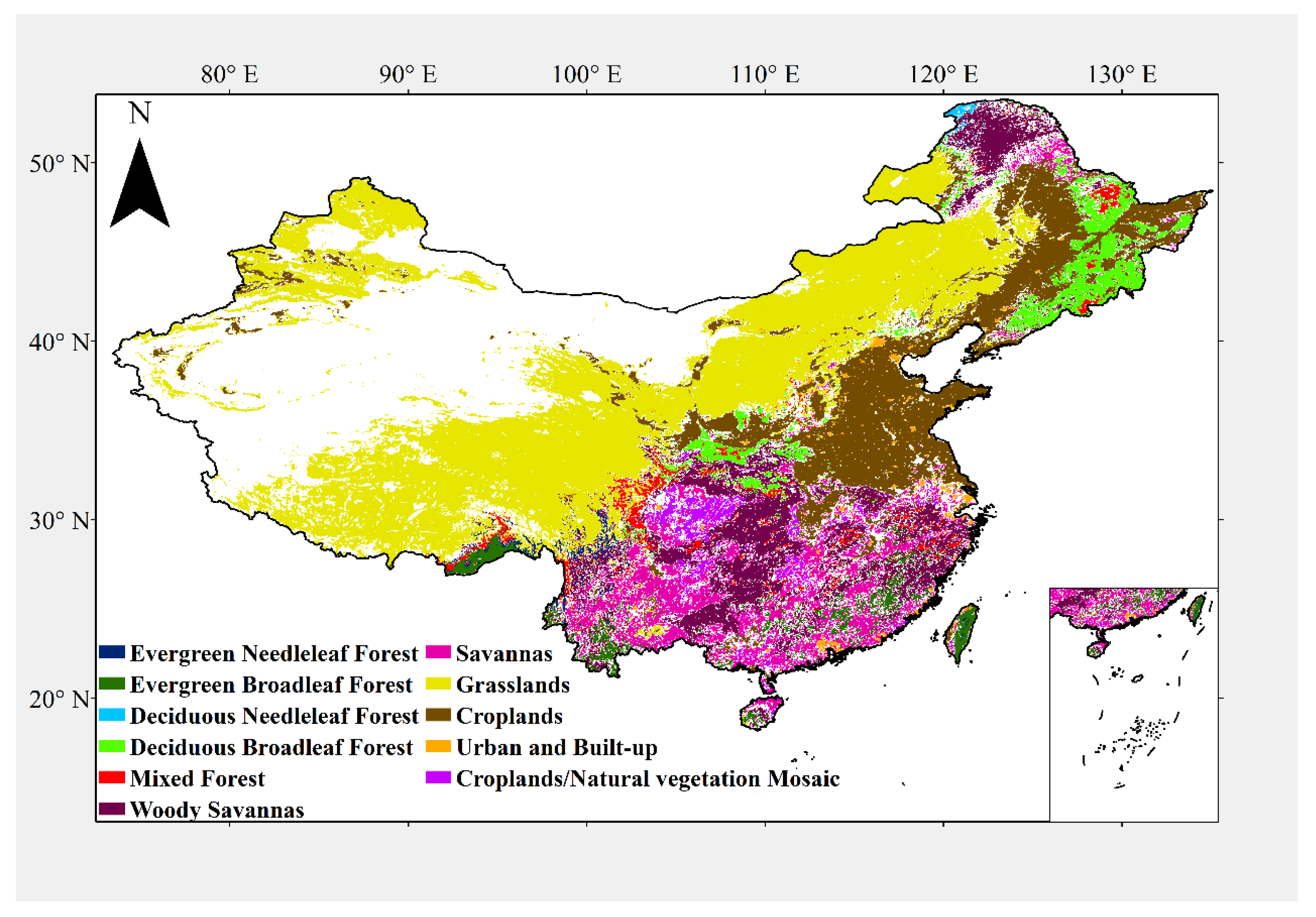
The 17-class International Geosphere-Biosphere Programme classification (IGBP) was adopted [44]. To reduce the possible influence of classification errors and land cover change, we also conducted land-cover-specific analyses [45]. In the land-cover-specific analyses, only the grids with the same dominant land cover class during 2001–2016 were kept back. The ‘closed shrublands’, ‘permanent wetlands’ and ‘open shrublands’ were excluded because they contained too few grids. The ‘water bodies’, ‘snow and ice’ and ‘barren or sparsely vegetated’ were also excluded because they had no or little vegetation cover. Finally, the land cover data used in this study contain eleven land cover classes (Figure 1), including Evergreen Needleleaf Forest (ENF), Evergreen Broadleaf Forest (EBF), Deciduous Needleleaf Forest (DNF), Deciduous Broadleaf Forest (DBF), Mixed Forest (MF), Woody Savannas (WS), Savannas (SAV), Grasslands (GRA), Croplands (CRO), Urban and Built-up (UB), Croplands/Natural vegetation Mosaic (CNM).
2.2. Methods of Analysis
All the analyses were performed using MATLAB (R2016b).
2.2.1. EEMD
The EEMD method decomposes nonlinear and nonstationary time series data into n intrinsic mode functions (IMF; imfi, i = 1, 2, …, n) and a secular trend. The decomposition process ‘sifting’ can be described as follows [30,31,32,33,34]:
Step 1: Add a Gaussian white noise series w1(t) to the original data x(t). The amplitude of the Gaussian white noise series was set to 0.2 times standard deviation of the original data.
Step 2: Form the upper and lower envelope curves of the time series data x1(t) by connecting local maxima and minima with cubic splines respectively; then the time series data x1(t) minus the mean value m1(t) of the upper and lower envelope curves.
Step 3: Determine whether f1(t) satisfies the given criterion (close enough to zero at anywhere). If yes, stop sifting. Otherwise, take f1(t) as a new time series data and repeat step 2. In this way, obtain the first IMF: imf1(t).
Step 4: Obtain the remainder R1(t) by subtracting imf1(t) from x1(t). If R1(t) still contains oscillatory component, repeat 2 and 3 but with R1(t) being the new time series data.
Thus, x1(t) is decomposed into n IMFs with decreasing frequencies and a residual trend that is monotonic or has at most one extremum.
Step 5: Repeat steps 1-4 for l times (l was set to 100 in this study) with different Gaussian white noise series added each time. Obtain the ensemble means of the corresponding IMFs and trends of the decompositions as the final results.
A MATLAB EEMD package with the stoppage criterion and end treatment is downloadable at http://rcada.ncu.edu.tw/research1.htm.
The EEMD trend of phenology series at a given time t is defined as the value increment of Rn from the beginning time 1981, that is:
For the trends that are time-varying, their changing rates are also temporally local quantities and can be calculated as:
Furthermore, we also conducted a significance test approach to test the EEMD trends. The detailed processes are as follows [34]: (1) generate 5000 white noise series with the same temporal length as the phenology series and implement EEMD to extract their secular trends; (2) divide the EEMD trends of that spatial location by the standard deviation of the corresponding phenology data; (3) find the 1.96 times standard deviation spread value of the trends of the white noise series as the 95% confidence interval; (4) judge whether the trend value is outside confidence interval.
The nonlinear trends interpreted by EEMD can be divided into five categories on the basis of their statistical significance [34].
Nonsignificant change: the trends were not significant at any year.
Monotonic Decrease/Monotonic Increase (the monotonic trends): the trend was monotonically increasing/decreasing and was statistical significant for at least one year. If a place displayed Monotonic Increase/Monotonic Decrease trend, it meant that SOS/EOS experienced delayed/advanced trend or LOS experienced prolonged/shortened trend.
Increase to Decrease/Decrease to Increase (the shifted trends): the trend contained one local maximum/minimum and was statistical significant for at least one year. If a place displayed Increase to Decrease trend, it meant that SOS/EOS delayed first and then turned to advance or LOS prolonged first and then turned to shortened. And if a place displayed Decrease to Increase trend, it meant that SOS/EOS advanced first and then turned to delay or LOS shortened first and then turned to prolonged.
We calculated the average of all pixels with the same latitude or longitude or land cover class to study the phenology trends from the angle of latitude, longitude and land cover class (Section 3.3, Figures 4–6). Moreover, a moving average over 0.5° in the latitudinal and longitudinal direction was used to eliminate possible noise. Function ‘contour’ in MATLAB was used to study phenology trends at different latitudes or longitudes and function ‘imagesc’ in MATLAB was used to study phenology trends at different land cover types.
2.2.2. Mann-Kendall Trend Test
In this study, Mann-Kendall trend test (M-K) was also used for trend analysis. Since this method does not require sample data to obey a certain distribution and is less affected by outliers, it can be used to effectively test the variation trend in time series [46].
The test statistic S is calculated by:
The standard normal variate Z is computed by:
Under the given significance level (P<0.05), there is a significant change if |Z| > Z1−α/2. When |Z| > 1.96, it means that the linear trend has passed the significance test of 0.05.
The linear trends interpreted by M–K were divided into three categories on the basis of their Z value.
Nonsignificant: Z value of the trend was between −1.96 and 1.96.
Significant Increase/ Significant Decrease: Z value of the trend was more than 1.96/less than −1.96. If a place displayed Significant Increase/ Significant Decrease trend, it meant that SOS/EOS experienced delayed/advanced trend or LOS experienced prolonged/shortened trend.
2.2.3. Linear Regression
We used the linear ordinary least squares regression method to calculate the average rate of phenology trends during the whole study period:
where t = 1, 2, 3, … , 36; y is value of phenology time series; α, β are the fitted intercept and slope, respectively; and ɛ refers to the error of the equation. A two-tailed t-test was used to verify the null hypothesis and examine the significance level of the trend.
3. Results
3.1. Vegetation Phenology Variation at the National Scale
As shown from Figure 2, the national average timing of SOS advanced at a rate of 0.22 d/yr (P < 0.01) during the period 1981–2016. The EEMD trend showed a significant advance (P < 0.05) during the whole period, while its rate gradually raised and exceeded the linear rate in the early-2000s. Meanwhile, the national average timing of EOS delayed at a rate of 0.20 d/yr (P < 0.01). The EEMD trends in EOS showed a significant delay (P < 0.05) during the whole period but its rate gradually shrank and dropped below the level of the linear rate in the later-1980s. Since LOS was determined by SOS and EOS together, the length of growing season prolonged for about 13 days at the end of our study period. The rate also displayed a significant increase trend and exceeded the linear rate in the early 21st century.
The linear trends in all phenological events showed the same tendency as the EEMD trends, which is an advanced SOS, a delayed EOS and a prolonged LOS. However, the rate of linear trends was stationary and that of EEMD trends was time-varying. The change rate of SOS became higher and higher than before, while that of EOS was just the opposite. Hence, it seemed that the increasing change rate of LOS might be mainly determined by SOS.
3.2. Spatial Pattern of Vegetation Phenology Trends
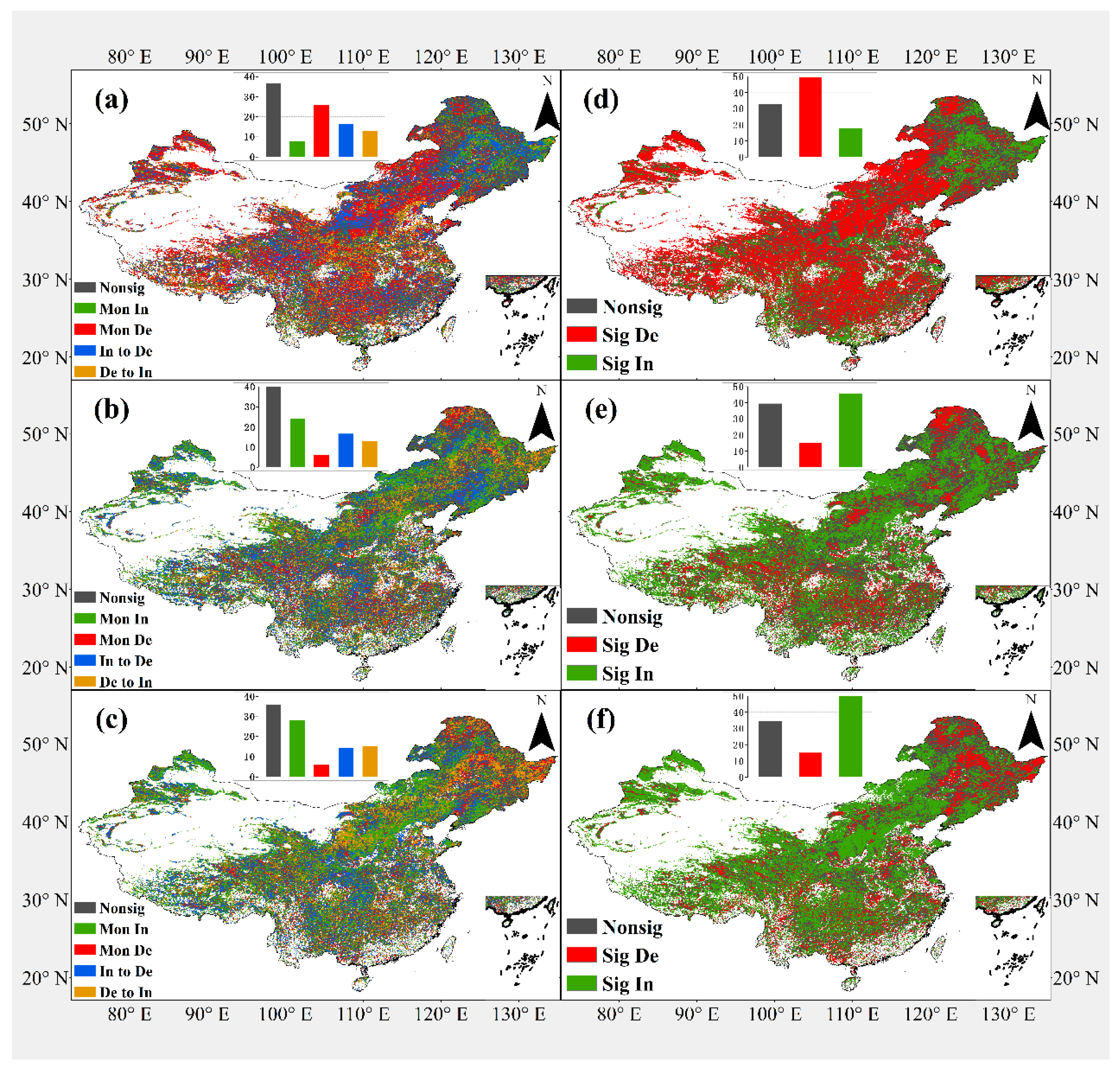
Figure 3 showed the spatial pattern of phenology trends, which was divided into five categories by EEMD (Nonsig, Monotonic Increase, Monotonic Decrease, Increase to Decrease and Decrease to Increase) and three by M–K (Nonsig, Significant Increase and Significant Decrease).
The EEMD and M–K outcome of each phenological event both suggested that the nonsignificant trends occupied the similar proportion of China (Table 1 and Table 2). For EEMD method, among the four significant trend types in SOS, monotonic decrease trends prevailed and occupied the largest area, while the regions that experienced monotonic increase trends were the smallest (Figure 3a). Moreover, there were two types of trend shifts (including Increase to Decrease and Decrease to Increase) in EEMD outcome which should not be ignored. Although their distribution was relatively scattered, roughly concentrated in the Loess Plateau, North China Plain and north-eastern China, each of their area percentages was more than monotonic decrease trends and less than monotonic increase trends, but their total percentages outnumbered that of monotonic increase trends (29.37% vs. 25.81%; Table 1). For EOS and LOS, monotonic increase trends occupied the largest area, while monotonic decrease trends occupied the smallest (Table 1 and Table 2). Moreover, the shifted trends in EOS and LOS were concentrated in the eastern Qinghai-Tibetan Plateau, eastern Sichuan Basin and north-eastern China, and eastern Sichuan Basin, Loess Plateau and north-eastern China, respectively (Figure 3b,c). Different from the EEMD outcome, as M–K method could not reveal the reversal of trends, there were only two significant trend types in the M–K outcome, without the two types of trend shifts. The area that experienced significant decrease trends in SOS was much larger than others (Figure 3d). The ratio of significant decrease trends was more than that of monotonic decrease trends from EEMD method. Meanwhile, the ratios of significant increase trends in EOS and LOS was much larger than others (Figure 3e,f). Considering the similar ratio of nonsignificant trends, it seems that a considerable part of shifted trends (i.e., Loess Plateau and north-eastern China) in EEMD was mistaken as significant decrease trends in M–K and thus the advance of SOS might be actually exaggerated. Similarly, there was also a considerable part of shifted trends in EOS (i.e., eastern Qinghai-Tibetan Plateau and eastern Sichuan Basin) and LOS (i.e., Loess Plateau and eastern Sichuan Basin) that was mistaken as significant increase trends, and thus the delay of EOS and the extension of LOS might be overstated.
It is clear that although considerable regions had the same phenology dynamics as the national overall trends (the advanced SOS, the delayed EOS and the prolonged LOS), the two methods agreed that the vegetation phenology trends in some regions of north-eastern China actually were the opposite (Figure 3). Furthermore, EEMD detected that the shifted trends mainly distributed in Loess Plateau, north-eastern China, eastern Qinghai-Tibetan Plateau and eastern Sichuan Basin. However, they were misunderstood in M–K as significant decrease/increase trends and thus the change rate of phenology might be enlarged.
3.3. Evolution of Vegetation Phenology Trends with Different Latitudes, Longitudes and Land Use Types
3.3.1. Evolution of Phenology Trends at Different Latitudes
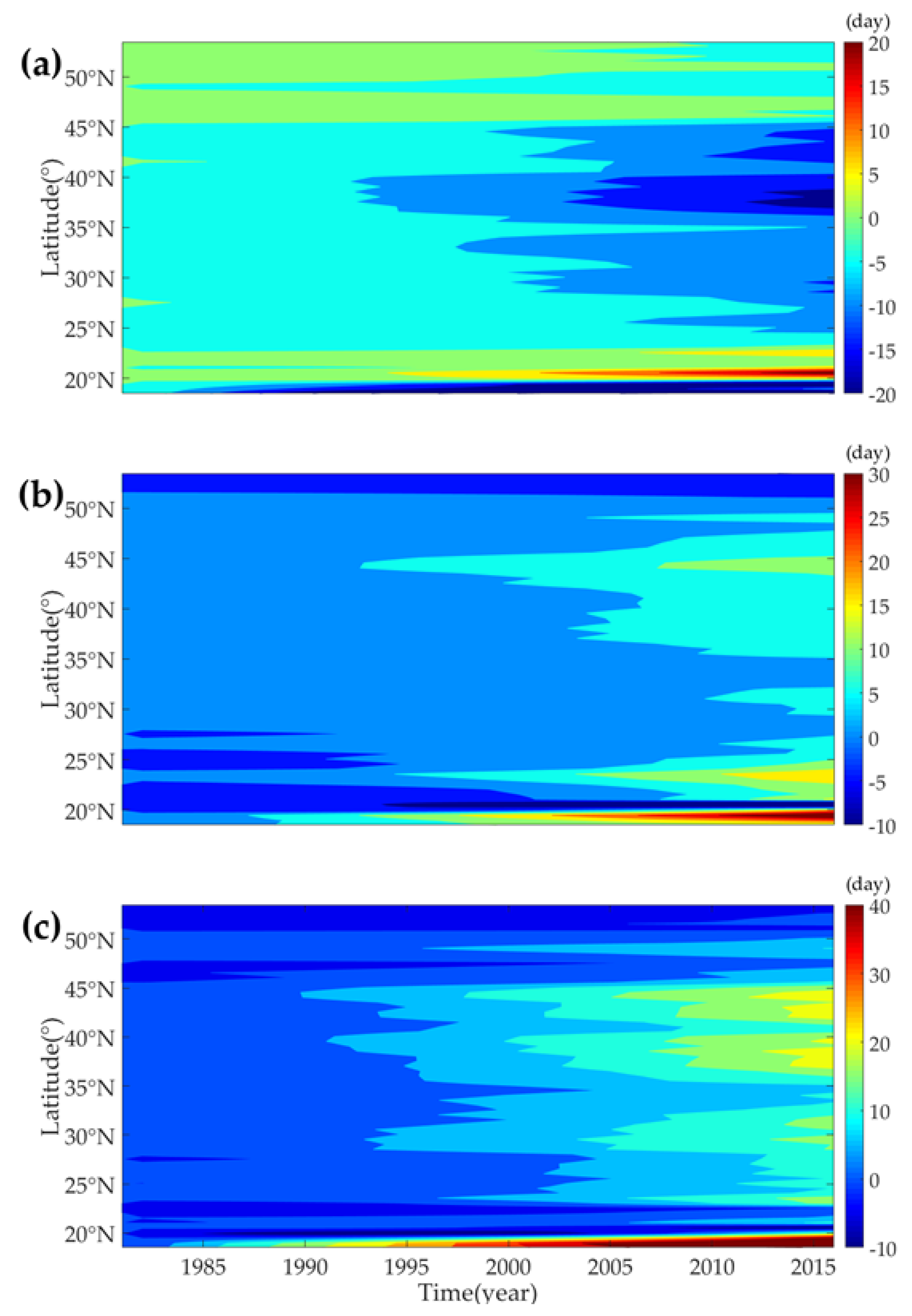
As seen from Figure 4, it was fairly clear that mid-latitude and low-latitude (south of the Tropic of Cancer) (between the Tropic of Cancer and 45°N) area experienced advanced SOS, delayed EOS and prolonged LOS. Nevertheless, the phenology dynamics in the high-latitude (north of 45°N) were just the opposite.
For SOS, the advance was starting at 40°N in the early-1990s and moving southward and northward, and the amplitude became greater after two or three times of advance. Meanwhile, the high-latitude area began to delay since the very beginning of the study period and the delayed amplitude was getting weaker, and even changed from delay to advance. However, there was a delayed trend occurring in a narrow band centered at 20°N and getting much stronger than before.
For EOS, considerable regions began to delay since the very beginning of the study period. But the evident delay appeared at 40°N in the early-1990s. The delayed amplitude became much stronger after two or three times of delay. Especially since the early-2000s, there was an enhancement in delay occurring in the southern low-latitude area. Meantime, there was a continuous advance occurring in the high-latitude, although its amplitude was extremely weak.
LOS has been prolonging in the mid-latitude since the early-1990s. By and large, the higher the latitude was, the earlier the extension of LOS appeared. Moreover, since the early 2000s, the extension has further increased. Meanwhile, the length of LOS in the high-latitude changed from decrease to increase. In the most area, there were about three or four time of extension of LOS. It was clearly that the change characteristics of LOS in the mid-latitude and low-latitude were closer to the sum of SOS and EOS, indicating that it may be mainly controlled by SOS and EOS in the mid-latitude and low-latitude. Meanwhile, LOS was mainly controlled by SOS in the high-latitude.
3.3.2. Evolution of Phenology Trends at Different Longitudes
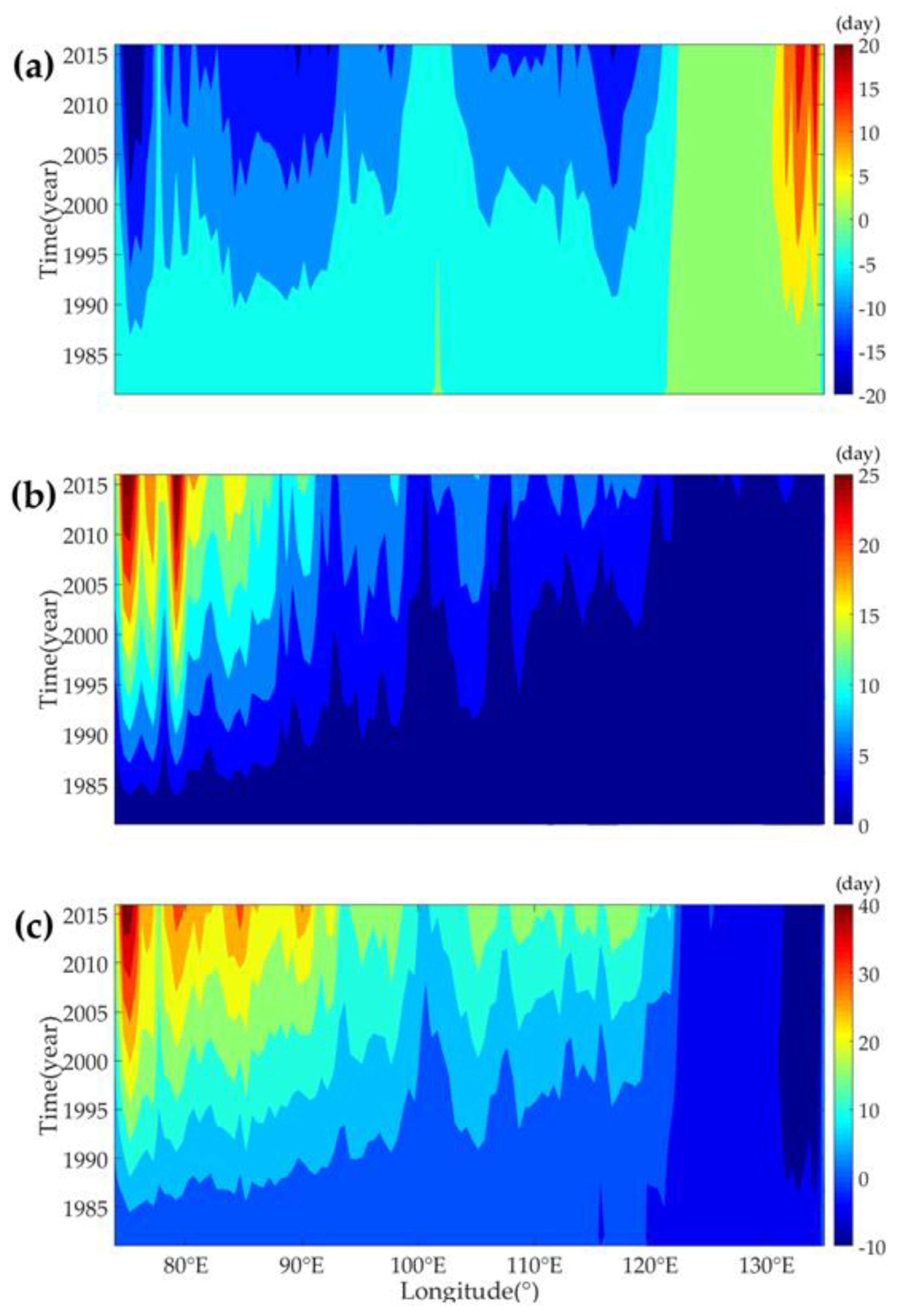
As can be seen from Figure 5, the amplitude of delay trends in EOS and prolonged trends in LOS increased with longitudes, while the beginning time of delay trends in EOS and prolonged trends in LOS decreased with longitudes. Meanwhile, it can be roughly divided into three regions, namely, eastern region (east of 121°E), central region (92°E–121°E) and western region (west of 92°E) based on the trends evolution of phenology varying with longitudes.
Although the eastern region experienced the same delayed EOS trends as the central and western regions, the trends in SOS and LOS were the opposite. That is that SOS delayed and LOS shortened in the eastern region, while SOS advanced and LOS prolonged in the central and western regions. Though the central and western regions experienced the same trends of phenology, their amplitudes and frequencies of trends variation with time were not the same. There were about two times of advance in SOS, four times of delay in EOS and five times of extension in LOS occurring in the western region. However, there were two times of advance in SOS, one time of delay in EOS and two times of extension in LOS occurring in the central region. The characteristics of the trends evolution of SOS and LOS in the eastern region were alike. The early characteristics of LOS in the central region was similar to those of SOS, while similar to those of EOS in the later. Meanwhile, the characteristics of LOS in the western region was similar to those of SOS and EOS. Hence, LOS was mainly induced by SOS in the east and by SOS and EOS in the west, respectively. Meanwhile, LOS in the central region was determined by SOS in the early stage and by EOS in the later stage.
3.3.3. Evolution of Phenology Trends at Different Land Cover Types
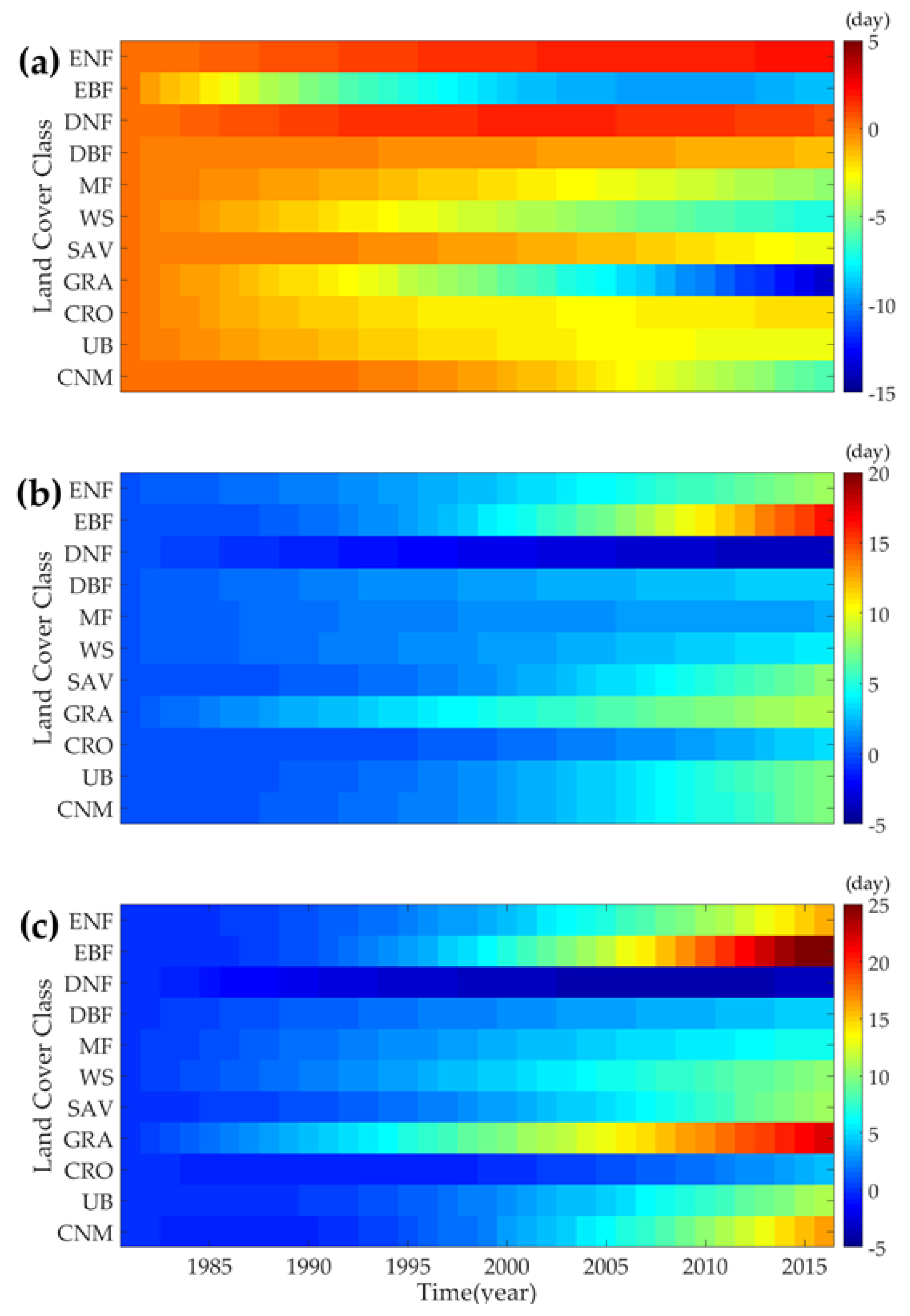
Figure 6 indicated that except Needleleaf forest (DNF and ENF), all other land cover types experienced the same trends as an advanced SOS, a delayed EOS and a prolonged LOS, though their evolution processes varied considerably. For SOS, most of the land cover types exhibited the advanced trends since mid-1990s and EBF was the earliest one. Moreover, except CRO, UB and ENF, other land cover types experienced several times of advance represented by different colors in Figure 6a. Meanwhile, GRA has the largest advanced amplitude. For EOS, GRA was the earliest one to exhibit obviously delayed trends, while EBF has the largest delayed days. Meanwhile, the delay of EOS began in 1990s for most land cover types, and experienced a continuously delayed trend, especially for GRA and EBF. Moreover, the ranges of other land cover types were all less than 10 days for both SOS and EOS, and mostly began to change since the late 1990s. Among them, the phenology trends of CRO was the most stable one, whose amplitude was always less than 5 days. The extension of LOS began in the later-1990s for most land cover types, except that GRA began in 1980s. For ENF, EBF, GRA and CNM, the extension of LOS was much larger than others, and experienced several times of variation.
4. Discussion
4.1. Evolution of the Vegetation Phenology Trends at the National Scale
Our study showed that over the whole China, the average vegetation phenology derived from EVI2 showed that SOS has advanced by 0.22 d/yr, EOS has delayed by 0.20 d/yr and thus LOS has lengthened by 0.42 d/yr during 1981–2016 (Figure 2). It is because that unprecedented global warming in the past several decades, especially in the past 20 years, may lead to earlier spring phenology and later autumn phenology, and thus further lengthened growing season [21]. The mean decrease rate of SOS estimated in our study was just a little smaller than Ma and Zhou (2.35 days per decade) and Ge et al. (2.75 days per decade) [20,22]. The spring phenology trend also generally agreed with that in Europe (2.5 days per decade) and in the Northern Hemisphere (2.8 days per decade) [21,47]. Meanwhile, our estimation in EOS was similar to Liu et al. (1.8 days per decade) and Jeong and Medvigy (2.4–3.6 days per decade) [23,48].
Ge et al. found that the advance of SOS became stronger since 1980s [22]. Our study suggested that not only the advance of SOS, but also the extension of LOS became stronger with EEMD method as time goes. Whereas the delay of EOS was getting weaker. Numerous studies suggested that warmer preseason (summer or autumn) temperatures delayed EOS and the preseason warming trends decelerated or even reversed in recent decades [15,48,49]. Hence, the rate of EOS was decreasing over the whole period. EEMD rate of SOS and LOS exceeded the linear rate in the early-2000s, while the EEMD rate of EOS dropped below the linear rate in the late-1980s. Hence, the variation of phenology trends over time seems to be largely nonlinear and more nonlinear methods like EEMD should be taken to detect the evolution of phenology trends [50].
4.2. Spatial Distribution of Different Types of Trends Evolution of Vegetation Phenology
Previous studies pointed out that the advance of SOS, delay of EOS, and extension of LOS are widely distributed in the world [5,15,22,48], which are consistent with the results of M-K method in our study. However, with EEMD method, the area that experienced Monotonic Decrease of SOS and Monotonic Increase of EOS and LOS were unexpectedly reduced. In the meanwhile, the shifted trends (including Increase to Decrease and Decrease to Increase) took up considerable area which were mostly from the main significant trends in M-K and have been ignored or misunderstood.
Our study found that North China Plain experienced Decrease to Increase of SOS and Loess Plateau experienced Increase to Decrease of SOS rather than continuous delayed trends reported by Ge et al. [22]. For EOS, we found that considerable area in north-eastern China and eastern Sichuan Basin experienced Increase to Decrease and some area in the eastern Qinghai-Tibetan Plateau experienced Monotonic Decrease and Increase to Decrease. Hence, the shifted trends mainly distributed in the north-eastern China, North China Plain, Loess Plateau, Sichuan Basin and Qinghai-Tibetan Plateau. For LOS, we found that the Increase to Decrease trends mainly occurred in eastern Sichuan Basin experienced, while the Decrease to Increase trends occurred in Loess Plateau and north-eastern China. These results show that the shifted trends did distribute widely in various regions, but were rarely mentioned in previous studies [15,22,26,50]. These discrepancies may be because that most traditional methods were linear and assumed that there were no trend shifts during the study period [34]. Without considering the potential trend shifts, the inherent trend shifts of vegetation phenology are completely ignored. Such neglect of trend shifts made the decrease trends in SOS change from 25.81% in EEMD to 49.87% in M-K the increase trends in EOS from 23.02% in EEMD to 44.89% in M-K, and the increase trends in LOS from 26.77% in EEMD to 48.24% in M-K. The nonlinear method, EEMD, can well reveal the trends evolution, and further extract the shifted trends which are usually ignored in linear methods. Therefore, we suggest that the trend shifts should be paid more attention with nonlinear methods to precisely reveal the trends of vegetation phenology including monotonic and shifted trends.
4.3. Vegetation Phenology Evolution with Different Latitudes, Longitude and Land Cover Types
Although previous studies have explored the spatial pattern of vegetation phenology [15,48,49,51], how the trends evolution of phenology along the latitudinal or longitudinal gradient was rarely reported. In our study, the amplitude and frequencies of the trends in all phenological events all evidently varied with latitude and longitude, especially with longitude.
From the angle of latitudinal gradient, the trends in the low and mid latitudes were exactly the opposite to those in the high-latitude. A delayed trend in SOS occurred in the high-latitude, while an advanced trend occurred in the low-latitude and mid-latitude weaker from 40°N to the north and south. Moreover, the frequencies of trends evolution were also getting less from 40°N to northward and southward. The delayed amplitude became much stronger after two or three times of delay in the mid-latitude. For EOS, an advanced trend occurred in the high-latitude, while a delayed trend occurred in the low-latitude and mid-latitude. Similarly, the frequencies of trends evolution were also getting less from 40°N to northward and southward. These differences might be related to the effect of temperature. In the high-latitude area in China, including middle temperate zone and sub-frigid zone, vegetation may not be able to fulfill the chilling requirements in a warmer winter and thus induce a later SOS [52,53]. Liu et al. found that EOS in the high-latitude area was positively correlated with precipitation but negatively with insolation, and thus reduced precipitation and increased insolation led to an earlier EOS and a shorter LOS [48]. While in the low-latitude and mid-latitude, including warm temperate and sub-tropics zone, the higher preseason temperatures could easily thaw frozen soil and bring earlier snow first melt and lead to an earlier SOS [5]. Moreover, higher temperatures in the summer and autumn may enhance photosynthetic activities, reduce the potential frost damage and the number of freezing days and thus induce, a later EOS and a longer LOS [50].
From the angle of longitudinal gradient, it was extremely clear that there was a dividing line between the eastern region and central region, whose longitude was approximately 121°E. The SOS outcome showed that the trends on both sides of 121°E were exactly the opposite. An advanced trend stronger from east to west occurred in the central and western region, while a delayed trend occurred in the east. Furthermore, the EOS outcome also showed that the magnitude of delay was stronger from east to west as longitudes changes. This phenomenon might be related to the effect of water stress on vegetation growth. For arid/semi-arid regions like the western and central regions in our study, water availability is the limiting factor for vegetation growth. Limited water availability would restrain vegetation growth and photosynthetic activities [54]. Under global warmer climate condition, more snow melt and earlier snow first melt may affect the timing of spring phenology [5,55]. Moreover, increased precipitation in the summer and autumn may mitigate water stress on vegetation in the western and central regions, and then promote vegetation activities and induce a later EOS [5,55]. Nevertheless, increased winter temperature and declined radiation brought by increased precipitation in the eastern region played a negative and more dominate role in determining vegetation growth and thus induced a later SOS and an earlier EOS respectively [51]. We also noticed that in some areas, such as areas near 35°N or 100°E, the variation amplitude of trends was unexpectedly weaker, which was consistent with Zheng et al. [56]. They discovered that the trends of spring phenology in the Weihe Plain and the west of Henan Province barely changed and concluded that the weak variation amplitude should be attributed to the nonsignificant temperature change and even decreased temperature.
Various results have confirmed that an earlier SOS is generally associated with a longer LOS [57,58]. However, a later EOS may also prolong LOS. Zhu et al. concluded that the prolonged LOS was mainly due to the delayed EOS in North America during the period 1982–2006 [59]. Our results suggested that LOS was mainly determined by SOS in the high-latitude, while LOS was collectively affected by SOS and EOS in the low-latitude and mid-latitude. Moreover, LOS was induced by SOS in the eastern region, while LOS was affected by SOS and EOS together in the western region. However, in the central region, LOS was controlled by SOS in the beginning and after the early-2000s, LOS became a joint effort of SOS and EOS. These results revealed that the effects of SOS and EOS on LOS may vary with location and time.
Studies have found that the spring phenology for herbaceous plants showed an overall advanced trend, while the advanced trends for woody plants were much stronger [48,60]. Our study detected from the angle of different land cover types that needle-leaf forests (DNF and ENF) experienced a later SOS and DNF experienced an earlier EOS and a shorter LOS, while SOS advanced, EOS delayed and LOS prolonged in all the other land cover types since 1980s, 1990s and later-1990s, respectively. We noticed that only needle-leaf forests experienced the delayed trends in SOS. This phenomenon was mainly caused by the winter-spring temperature increasing. As needle-leaf forests were low-temperature vegetation widely concentrated in the high-latitude cold zone, they might not fulfill the chilling requirements in a warmer winter [5]. Though all the other land cover types experienced the same trends, their evolution processes varied considerably. For EBF and GRA, their amplitudes and frequencies of phenology variation were more than others, while CRO just had little small amplitude and nonsignificant trend evolution. This may be because that CRO is greatly managed by human and thus the response of CRO to climate change may be different from other vegetation. GRA mainly located in the mid-latitude temperate zone, a warmer winter may break the ecodormancy and thus an earlier SOS [5]. EBF mainly located in the mid-and low latitude subtropical zone, higher temperatures in the summer and autumn may enhance activities of photosynthetic enzymes and slow the speed of chlorophyll degradation [48,51]. These results suggested that different species showed the same trends but diverse trend evolution of phenology variation under global warming.
4.4. Limitation and Future Direction
Our results are subject to some caveats. First, the phenology dataset used in the study is at a spatial resolution of 0.05° extracted from EVI2, which can be coarse for some areas. However, this dataset is still likely the best one we can currently use for a large-scale analysis. The dataset is composed of three widely-used satellites and hence it has covers a relative long time period, though it has a lower spatial resolution. Future development of higher-resolution satellite dataset may help us deepen understanding of the evolution of phenology trends. Second, we aimed to seek the effects of geographical factors on phenology trends and we did find that the difference exists in both latitudinal and longitudinal direction. This means that latitude and longitude are two suitable variables for analyzing the spatial pattern of vegetation phenology trends at a national scale. But considering the impact of Eastern Asia Monsoon, Westerlies and etc., the climatic factors (i.e., precipitation) are not strictly varying with geographical factors (i.e., longitude). Future studies should take both geographical factors and climatic factors and their interaction into consideration.
5. Conclusions
The EEMD results showed that the change rates of SOS and LOS were increasing with time, while that of EOS was decreasing. Moreover, the EEMD rates of SOS and LOS exceeded the linear rate in the early-2000s, while that of EOS exceeded the linear rate in the mid-1980s. Hence, EEMD method is able to well reveal the nonlinearity of phenology trends. Although a large regions experienced the advance of SOS, the delay of EOS and the extension of LOS, EEMD detected a large proportion of the shifted trends while M-K did not. All three phenological events showed latitudinal and longitudinal gradients, while longitudinal gradient was much stronger, especially in EOS. The area located in the mid-latitude and low-latitude displayed the same trends as the overall trends on the national scale, while the areas in the high-latitude experienced the contrary trends. The amplitudes and frequencies of phenology variation in the mid-latitude were stronger than those in the high-latitude and low-latitude. Areas in the western and central region experienced an advanced SOS trend and a prolonged LOS trend during the whole study period, which was contrary to the eastern region. The magnitude of delayed trends in EOS was stronger from east to west as longitudes change, while the beginning time decreased with longitudes. LOS was mostly determined by SOS in the high-latitude and the eastern region, while LOS was induced collectively by SOS and EOS in the mid-latitude, low-latitude and western region. Moreover, in the central region, LOS was controlled by SOS in the beginning and after the early-2000s, LOS became a joint effort of SOS and EOS. Almost all land cover types, except Needleleaf forests, experienced the advance of SOS, delay of EOS and extension of LOS. Among them, the magnitude of GRA and EBF was biggest one in SOS and EOS, respectively. Whereas, the amplitude of CRO was smallest one in all phenological events. As a time-varying analyses method, EEMD displayed the evolution of vegetation phenology dynamics and the spatial pattern of the shift trends. Thus, EEMD method is capable of better detecting temporal variation and hidden shift trends than traditional linear method.
Author Contributions
Conceptualization, H.L.; Data curation, F.J.; Formal analysis, F.J. and X.X; Funding acquisition, H.L. and Z.L.; Investigation, F.J.; Methodology, F.J. and X.X.; Project administration, H.L. and Z.L.; Resources, F.J.; Software, F.J.; Supervision, H.L.; Visualization, F.J. and H.G.; Writing—original draft, F.J.; Writing—review & editing, H.L. All authors have read and agreed to the published version of the manuscript.
Funding
This research was funded by National Natural Science Foundation of China (No. 41971382, 31470519) and the Priority Academic Program Development of Jiangsu Higher Education Institutions (164320H116).
Conflicts of Interest
The authors declare no conflict of interest.
References
- Lieth, H. Phenology and Seasonal Modeling; Springer: Heidelberg, Germany, 1974. [Google Scholar]
- Schwartz, M.D. Phenology: An Integrative Environmental Science; Springer: Dordrecht, The Netherlands, 2003. [Google Scholar]
- Intergovernmental Panel on Climate Change. Climate Change 2007—Mitigation of Climate Change: Working Group III contribution to the Fourth Assessment Report of the IPCC; Cambridge University Press: Cambridge, UK, 2008. [Google Scholar]
- Intergovernmental Panel on Climate Change. Climate Change 2013—The Physical Science Basis: Working Group I Contribution to the Fifth Assessment Report of the Intergovernmental Panel on Climate Change; Cambridge University Press: Cambridge, UK, 2014. [Google Scholar]
- Piao, S.; Liu, Q.; Chen, A.; Janssens, I.A.; Fu, Y.; Dai, J.; Liu, L.; Lian, X.; Shen, M.; Zhu, X. Plant phenology and global climate change: Current progresses and challenges. Glob. Chang. Biol. 2019, 25, 1922–1940. [Google Scholar] [CrossRef] [PubMed]
- De Beurs, K.M.; Henebry, G.M. Land surface phenology and temperature variation in the International Geosphere-Biosphere Program high-latitude transects. Glob. Chang. Boil. 2005, 11, 779–790. [Google Scholar] [CrossRef]
- Yu, H.; Xu, J.; Okuto, E.; Luedeling, E. Seasonal Response of Grasslands to Climate Change on the Tibetan Plateau. PLoS ONE 2012, 7, e49230. [Google Scholar] [CrossRef] [PubMed]
- Zhang, X.; Tan, B.; Yu, Y. Interannual variations and trends in global land surface phenology derived from enhanced vegetation index during 1982–2010. Int. J. Biometeorol. 2014, 58, 547–564. [Google Scholar] [CrossRef] [Green Version]
- Sparks, T.; Carey, P.D. The Responses of Species to Climate Over Two Centuries: An Analysis of the Marsham Phenological Record, 1736–1947. J. Ecol. 1995, 83, 321–329. [Google Scholar] [CrossRef]
- Aono, Y.; Kazui, K. Phenological data series of cherry tree flowering in Kyoto, Japan, and its application to reconstruction of springtime temperatures since the 9th century. Int. J. Climatol. 2008, 28, 905–914. [Google Scholar] [CrossRef] [Green Version]
- Moulin, S.; Kergoat, L.; Viovy, N.; Dedieu, G. Global-Scale Assessment of Vegetation Phenology Using NOAA/AVHRR Satellite Measurements. J. Clim. 1995, 10, 1154–1170. [Google Scholar] [CrossRef]
- Ganguly, S.; Friedl, M.A.; Tan, B.; Zhang, X.; Verma, M. Land surface phenology from MODIS: Characterization of the Collection 5 global land cover dynamics product. Remote Sens. Environ. 2010, 114, 1805–1816. [Google Scholar] [CrossRef] [Green Version]
- Zhang, X.; Friedl, M.A.; Schaaf, C.B.; Strahler, A.H.; Hodges, J.C.; Gao, F.; Reed, B.C.; Huete, A. Monitoring vegetation phenology using MODIS. Remote Sens. Environ. 2003, 84, 471–475. [Google Scholar] [CrossRef]
- White, M.A.; Thornton, P.E.; Running, S.W. A continental phenology model for monitoring vegetation responses to interannual climatic variability. Glob. Biogeochem. Cycles 1997, 11, 217–234. [Google Scholar] [CrossRef]
- Piao, S.; Fang, J.; Zhou, L.; Ciais, P.; Zhu, B. Variations in satellite-derived phenology in China’s temperate vegetation. Glob. Chang. Boil. 2006, 12, 672–685. [Google Scholar] [CrossRef]
- Myneni, R.B.; Tucker, C.J.; Asrar, G.; Keeling, C.D. Interannual variations in satellite-sensed vegetation index data from 1981 to 1991. J. Geophys. Res. Space Phys. 1998, 103, 6145–6160. [Google Scholar] [CrossRef] [Green Version]
- Jiang, Z.; Huete, A.R.; Didan, K.; Miura, T. Development of a two-band enhanced vegetation index without a blue band. Remote Sens. Environ. 2008, 112, 3833–3845. [Google Scholar] [CrossRef]
- de Beurs, K.M.; Henebry, G.M. Land surface phenology, climatic variation, and institutional change: Analyzing agricultural land cover change in Kazakhstan. Remote Sens. Environ. 2004, 89, 497–509. [Google Scholar] [CrossRef]
- Cleland, E.E.; Chuine, I.; Menzel, A.; Mooney, H.A.; Schwartz, M.D. Shifting plant phenology in response to global change. Trends Ecol. Evol. 2007, 22, 357–365. [Google Scholar] [CrossRef] [PubMed]
- Menzel, A.; Sparks, T.H.; Estrella, N.; Koch, E.; Aasa, A.; Ahas, R.; Alm-Kübler, K.; Bissolli, P.; Braslavská, O.; Briede, A.; et al. European phenological response to climate change matches the warming pattern. Glob. Chang. Boil. 2006, 12, 1969–1976. [Google Scholar] [CrossRef]
- Ge, Q.; Wang, H.; Rutishauser, T.; Dai, J. Phenological response to climate change in China: A meta-analysis. Glob. Chang. Biol. 2015, 21, 265–274. [Google Scholar] [CrossRef]
- Jeong, S.J.; Medvigy, D. Macroscale prediction of autumn leaf coloration throughout the continental United States. Glob. Ecol. Biogeogr. 2014, 23, 1245–1254. [Google Scholar] [CrossRef]
- Pan, N.; Feng, X.; Fu, B.; Wang, S.; Ji, F.; Pan, S. Increasing global vegetation browning hidden in overall vegetation greening: Insights from time-varying trends. Remote Sens. Environ. 2018, 214, 59–72. [Google Scholar] [CrossRef]
- Wang, X.; Piao, S.; Xu, X.; Ciais, P.; MacBean, N.; Myneni, R.B.; Li, L. Has the advancing onset of spring vegetation green-up slowed down or changed abruptly over the last three decades? Glob. Ecol. Biogeogr. 2015, 24, 621–631. [Google Scholar] [CrossRef]
- Wang, X.; Piao, S.; Ciais, P.; Li, J.; Friedlingstein, P.; Koven, C.; Chen, A. Spring temperature change and its implication in the change of vegetation growth in North America from 1982 to 2006. Proc. Natl. Acad. Sci. USA 2011, 108, 1240–1245. [Google Scholar] [CrossRef] [PubMed] [Green Version]
- Tian, F.; Fensholt, R.; Verbesselt, J.; Grogan, K.; Horion, S.; Wang, Y. Evaluating temporal consistency of long-term global NDVI datasets for trend analysis. Remote Sens. Environ. 2015, 163, 326–340. [Google Scholar] [CrossRef]
- Verbesselt, J.; Hyndman, R.; Newnham, G.; Culvenor, D. Detecting trend and seasonal changes in satellite image time series. Remote Sens. Environ. 2010, 114, 106–115. [Google Scholar] [CrossRef]
- de Jong, R.; Verbesselt, J.; Schaepman, M.E.; De Bruin, S. Trend changes in global greening and browning: Contribution of short-term trends to longer-term change. Glob. Chang. Biol. 2012, 18, 642–655. [Google Scholar] [CrossRef]
- Wu, Z.; Huang, N.E. Ensemble empirical mode decomposition: A noise-assisted data analysis method. Adv. Adapt. Data Anal. 2009, 1, 1–41. [Google Scholar] [CrossRef]
- Huang, N.E.; Wu, Z. A review on Hilbert-Huang transform: Method and its applications to geophysical studies. Rev. Geophys. 2008, 46, RG2006. [Google Scholar] [CrossRef] [Green Version]
- Huang, N.E.; Shen, Z.; Long, S.R.; Wu, M.C.; Shih, H.H.; Zheng, Q.; Yen, N.-C.; Tung, C.C.; Liu, H.H. The empirical mode decomposition and the Hilbert spectrum for nonlinear and non-stationary time series analysis. Proc. R. Soc. A Math. Phys. Eng. Sci. 1998, 454, 903–995. [Google Scholar] [CrossRef]
- Ji, F.; Wu, Z.; Huang, J.; Chassignet, E.P. Evolution of land surface air temperature trend. Nat. Clim. Chang. 2014, 4, 462–466. [Google Scholar] [CrossRef]
- Guan, B.T. Ensemble empirical mode decomposition for analyzing phenological responses to warming. Agric. For. Meteorol. 2014, 194, 1–7. [Google Scholar] [CrossRef]
- Hawinkel, P.; Swinnen, E.; Lhermitte, S.; Verbist, B.; Van Orshoven, J.; Muys, B. A time series processing tool to extract climate-driven interannual vegetation dynamics using Ensemble Empirical Mode Decomposition (EEMD). Remote Sens. Environ. 2015, 169, 375–389. [Google Scholar] [CrossRef] [Green Version]
- Yin, Y.; Ma, D.; Wu, S.; Dai, E.; Zhu, Z.; Myneni, R.B. Nonlinear variations of forest leaf area index over China during 1982–2010 based on EEMD method. Int. J. Biometeorol. 2017, 61, 977–988. [Google Scholar] [CrossRef] [PubMed]
- Liu, H.; Zhang, M.; Lin, Z. Relative importance of climate changes at different time scales on net primary productivity—A case study of the Karst area of northwest Guangxi, China. Environ. Monit. Assess. 2017, 189, 539. [Google Scholar] [CrossRef] [PubMed]
- Liu, H.; Zhang, M.; Lin, Z.; Xu, X. Spatial heterogeneity of the relationship between vegetation dynamics and climate change and their driving forces at multiple time scales in Southwest China. Agric. For. Meteorol. 2018, 256, 10–21. [Google Scholar] [CrossRef]
- Didan, K. Multi-satellite Earth science data record for studying global vegetation trends and changes. IEEE Int. Geosci. Remote Sens. Symp. 2014, 2530, 2530. [Google Scholar]
- Jönsson, P.; Eklundh, L. TIMESAT—A program for analyzing time-series of satellite sensor data. Comput. Geosci. 2004, 30, 833–845. [Google Scholar] [CrossRef] [Green Version]
- Vorobiova, N.; Chernov, A. Curve fitting of MODIS NDVI time series in the task of early crops identification by satellite images. Procedia Eng. 2017, 201, 184–195. [Google Scholar] [CrossRef]
- Friedl, M.A.; Sulla-Menashe, D.; Tan, B.; Schneider, A.; Ramankutty, N.; Sibley, A.; Huang, X. MODIS Collection 5 global land cover: Algorithm refinements and characterization of new datasets. Remote. Sens. Environ. 2010, 114, 168–182. [Google Scholar] [CrossRef]
- Loveland, T.R.; Belward, A.S. The IGBP-DIS global 1km land cover data set, DISCover: First results. Int. J. Remote Sens. 1997, 18, 3289–3295. [Google Scholar] [CrossRef]
- Forzieri, G.; Alkama, R.; Miralles, D.G.; Cescatti, A. Satellites reveal contrasting responses of regional climate to the widespread greening of Earth. Science 2017, 356, 1180–1184. [Google Scholar] [CrossRef] [Green Version]
- Yu, Y.S.; Zou, S.; Whittemore, D. Non-parametric trend analysis of water quality data of rivers in Kansas. J. Hydrol. 1993, 150, 61–80. [Google Scholar] [CrossRef]
- Ma, T.; Zhou, C.G. Climate-associated changes in spring plant phenology in China. Int. J. Biometeorol. 2012, 56, 269–275. [Google Scholar] [CrossRef] [PubMed]
- Parmesan, C. Influences of species, latitudes and methodologies on estimates of phenological response to global warming. Glob. Chang. Biol. 2007, 13, 1860–1872. [Google Scholar] [CrossRef]
- Liu, Q.; Fu, Y.H.; Zeng, Z.; Huang, M.; Li, X.; Piao, S. Temperature, precipitation, and insolation effects on autumn vegetation phenology in temperate China. Glob. Chang. Biol. 2016, 22, 644–655. [Google Scholar] [CrossRef] [PubMed]
- Yang, Y.; Guan, H.; Shen, M.; Liang, W.; Jiang, L. Changes in autumn vegetation dormancy onset date and the climate controls across temperate ecosystems in China from 1982 to 2010. Glob. Chang. Biol. 2015, 21, 652–665. [Google Scholar] [CrossRef]
- Fu, Y.H.; Zhao, H.; Piao, S.; Peaucelle, M.; Peng, S.; Zhou, G.; Ciais, P.; Huang, M.; Menzel, A.; Peñuelas, J.; et al. Declining global warming effects on the phenology of spring leaf unfolding. Nature 2015, 526, 104–107. [Google Scholar] [CrossRef] [Green Version]
- Shi, C.; Sun, G.; Zhang, H.; Xiao, B.; Ze, B.; Zhang, N.; Wu, N. Effects of Warming on Chlorophyll Degradation and Carbohydrate Accumulation of Alpine Herbaceous Species during Plant Senescence on the Tibetan Plateau. PLoS ONE 2014, 9, e107874. [Google Scholar] [CrossRef]
- Wu, C.; Hou, X.; Peng, D.; Gonsamo, A.; Xu, S.; Peng, L. Land surface phenology of China’s temperate ecosystems over 1999–2013: Spatial–temporal patterns, interaction effects, covariation with climate and implications for productivity. Agric. Meteorol. 2016, 216, 177–187. [Google Scholar] [CrossRef]
- Piao, S.; Ciais, P.; Huang, Y.; Shen, Z.; Peng, S.; Li, J.; Zhou, L.; Liu, H.; Ma, Y.; Ding, Y.; et al. The impacts of climate change on water resources and agriculture in China. Nature 2010, 467, 43–51. [Google Scholar] [CrossRef]
- Yu, H.; Luedeling, E.; Chapin, J. Winter and spring warming result in delayed spring phenology on the Tibetan Plateau. Proc. Natl. Acad. Sci. USA 2010, 107, 22151–22156. [Google Scholar] [CrossRef] [Green Version]
- Tezara, W.; Mitchell, V.J.; Driscoll, S.D.; Lawlor, D.W. Water stress inhibits plant photosynthesis by decreasing coupling factor and ATP. Nature 1999, 401, 914–917. [Google Scholar] [CrossRef]
- Wang, Y.; Qin, D. Influence of climate change and human activity on water resources in arid region of Northwest China: An overview. Adv. Clim. Chang. Res. 2017, 8, 268–278. [Google Scholar] [CrossRef]
- Zheng, J.; Ge, Q.; Hao, Z. Impacts of climate warming on plants phenophases in China for the last 40 years. Chin. Sci. Bull. 2002, 47, 1826–1831. [Google Scholar] [CrossRef]
- Wu, C.; Chen, J.M.; Gonsamo, A.; Price, D.T.; Black, T.A.; Kurz, W.A. Interannual variability of net carbon exchange is related to the lag between the end-dates of net carbon uptake and photosynthesis: Evidence from long records at two contrasting forest stands. Agric. Meteorol. 2012, 164, 29–38. [Google Scholar] [CrossRef]
- Myneni, R.B.; Keeling, C.D.; Tucker, C.J.; Asrar, G.; Nemani, R.R. Increased plant growth in the northern high latitudes from 1981 to 1991. Nature 1997, 386, 698–702. [Google Scholar] [CrossRef]
- Zhu, W.; Tian, H.; Xu, X.; Pan, Y.; Chen, G.; Lin, W. Extension of the growing season due to delayed autumn over mid and high latitudes in North America during 1982–2006. Glob. Ecol. Biogeogr. 2012, 21, 260–271. [Google Scholar] [CrossRef]
- Zheng, Z.; Zhu, W.; Chen, G.; Jiang, N.; Fan, D.; Zhang, D. Continuous but diverse advancement of spring-summer phenology in response to climate warming across the Qinghai-Tibetan Plateau. Agric. Meteorol. 2016, 223, 194–202. [Google Scholar] [CrossRef]
Figure 1.
Selected land cover map of China from MODIS MCD12C1 products from 2001–2016.

Figure 2.
The left three are the mean SOS, EOS and LOS and their EEMD and linear trends. The green solid line and red dotted line indicate the EEMD trend and the linear trend, respectively. The right three are the linear rates of SOS, EOS and LOS and their EEMD trend rates. The green solid line and red dotted line indicate the EEMD trend rates and the linear trend rates, respectively.

Figure 3.
The spatial pattern of different types of phenology trends. (a–c) show the spatial pattern estimated by EEMD of SOS, EOS and LOS, respectively. (d–f) show the spatial pattern estimated by M-K of SOS, EOS and LOS, respectively. ‘Nonsig’, ‘Mon In’, ‘Mon De’, ‘In to De’ and ‘De to In’ are abbreviations for ‘Nonsignificant’, ‘Monotonic Increase’, ‘Monotonic Decrease’, ‘Increase to Decrease’ and ‘Decrease to Increase’.

Figure 4.
Variation of the trends estimated by EEMD in each latitudinal band. (a–c) show the results of SOS, EOS and LOS, respectively. In each subfigure, a moving average over 0.5° in the meridional direction was used to eliminate possible noise.
Figure 4.
Variation of the trends estimated by EEMD in each latitudinal band. (a–c) show the results of SOS, EOS and LOS, respectively. In each subfigure, a moving average over 0.5° in the meridional direction was used to eliminate possible noise.

Figure 5.
Variation of the trends estimated by EEMD in each longitudinal band. (a–c) show the results of SOS, EOS and LOS, respectively. In each subfigure, an average over 0.5° in the equatorial direction was used to eliminate possible noise.
Figure 5.
Variation of the trends estimated by EEMD in each longitudinal band. (a–c) show the results of SOS, EOS and LOS, respectively. In each subfigure, an average over 0.5° in the equatorial direction was used to eliminate possible noise.

Figure 6.
Variation of the trends with time estimated by EEMD in each land cover type. (a–c) show the results of SOS, EOS and LOS, respectively.
Figure 6.
Variation of the trends with time estimated by EEMD in each land cover type. (a–c) show the results of SOS, EOS and LOS, respectively.


Table 1.
The area percentage of different types of phenology trends by EEMD. ‘Nonsig’, ‘Mon In’, ‘Mon De’, ‘In to De’ and ‘De to In’ are abbreviations for ‘Nonsignificant’, ‘Monotonic Increase’, ‘Monotonic Decrease’, ‘Increase to Decrease’ and ‘Decrease to Increase’.
Table 1.
The area percentage of different types of phenology trends by EEMD. ‘Nonsig’, ‘Mon In’, ‘Mon De’, ‘In to De’ and ‘De to In’ are abbreviations for ‘Nonsignificant’, ‘Monotonic Increase’, ‘Monotonic Decrease’, ‘Increase to Decrease’ and ‘Decrease to Increase’.
| SOS | EOS | LOS | |
|---|---|---|---|
| Nonsig | 36.65% | 39.13% | 34.19% |
| Mon In | 8.17% | 23.02% | 26.77% |
| Mon De | 25.81% | 5.74% | 5.69% |
| In to De | 16.38% | 16.24% | 13.65% |
| De to In | 12.99% | 12.95% | 14.42% |
Table 2.
The area percentage of different types of phenology trends by M-K. ‘Nonsig’, ‘Sig De’ and ‘Sig In’ are abbreviations for ‘Nonsignificant’ (Nonsignificant Decrease and Increase), ‘Significant Decrease’ and ‘Significant Decrease’.
Table 2.
The area percentage of different types of phenology trends by M-K. ‘Nonsig’, ‘Sig De’ and ‘Sig In’ are abbreviations for ‘Nonsignificant’ (Nonsignificant Decrease and Increase), ‘Significant Decrease’ and ‘Significant Decrease’.
| SOS | EOS | LOS | |
|---|---|---|---|
| Nonsig | 33.14% | 38.74% | 32.80% |
| Sig De | 49.87% | 14.81% | 14.27% |
| Sig In | 17.77% | 44.89% | 48.24% |
© 2020 by the authors. Licensee MDPI, Basel, Switzerland. This article is an open access article distributed under the terms and conditions of the Creative Commons Attribution (CC BY) license (http://creativecommons.org/licenses/by/4.0/).
Share and Cite
MDPI and ACS Style
Jiao, F.; Liu, H.; Xu, X.; Gong, H.; Lin, Z. Trend Evolution of Vegetation Phenology in China during the Period of 1981–2016. Remote Sens. 2020, 12, 572. https://0-doi-org.brum.beds.ac.uk/10.3390/rs12030572
AMA Style
Jiao F, Liu H, Xu X, Gong H, Lin Z. Trend Evolution of Vegetation Phenology in China during the Period of 1981–2016. Remote Sensing. 2020; 12(3):572. https://0-doi-org.brum.beds.ac.uk/10.3390/rs12030572
Chicago/Turabian StyleJiao, Fusheng, Huiyu Liu, Xiaojuan Xu, Haibo Gong, and Zhenshan Lin. 2020. "Trend Evolution of Vegetation Phenology in China during the Period of 1981–2016" Remote Sensing 12, no. 3: 572. https://0-doi-org.brum.beds.ac.uk/10.3390/rs12030572
Note that from the first issue of 2016, this journal uses article numbers instead of page numbers. See further details here.