A Method for Vehicle Detection in High-Resolution Satellite Images that Uses a Region-Based Object Detector and Unsupervised Domain Adaptation

Abstract

Recently, object detectors based on deep learning have become widely used for vehicle detection and contributed to drastic improvement in performance measures. However, deep learning requires much training data, and detection performance notably degrades when the target area of vehicle detection (the target domain) is different from the training data (the source domain). To address this problem, we propose an unsupervised domain adaptation (DA) method that does not require labeled training data, and thus can maintain detection performance in the target domain at a low cost. We applied Correlation alignment (CORAL) DA and adversarial DA to our region-based vehicle detector and improved the detection accuracy by over 10% in the target domain. We further improved adversarial DA by utilizing the reconstruction loss to facilitate learning semantic features. Our proposed method achieved slightly better performance than the accuracy achieved with the labeled training data of the target domain. We demonstrated that our improved DA method could achieve almost the same level of accuracy at a lower cost than non-DA methods with a sufficient amount of labeled training data of the target domain.

1. Introduction

Recently, vehicle detection methods have been drastically improving due to the use of deep learning. A current prevalent method uses a region-based detector, which searches possible object locations based on image features and classifies them by using a convolutional neural network (CNN). The deep learning method requires adequate training to achieve high levels of accuracy. Although several large-scale open datasets for vehicle detection have been proposed, the region of interest (RoI) in practice (the “target domain”) is often different from that in the datasets (the “source domain”). In such cases, vehicle detection performance in the target domain is notably low because of differences in image features between the source and target domains. Although the method of Tang et al. [1] could achieve high accuracy in the source domain (Munich dataset), that method could not address the image feature difference between the source and the target (collected vehicle dataset) domain; thus, the accuracy in the target domain was notably lower than the source domain. To achieve a useful level of accuracy, additional training data are required in the target domain, but adding this step is quite costly.

Domain adaptation (DA) is a solution used to address this problem. A general objective of DA is to find the common feature space of source and target domains and align the features in unsupervised ways. A conventional approach is distribution matching, where the statistical distance between examples of the source and target domains are calculated, and a common feature space that minimizes the distance is identified [2]. For example, a transformation matrix that minimizes the distance between source and target examples can be calculated, and the features transformed by the matrix are classified by a classifier such as a support vector machine [3]. Despite its potential benefits, the application of DA to vehicle detection has not yet been explored.

In this paper, we applied the DA method to a region-based object detector for vehicle detection and demonstrated that DA methods can significantly improve accuracy in a target domain at a low cost. Our contributions in this paper are as follows:

(a) We adapted two domain adaptation methods that were originally proposed for image classification networks to an object detection network and applied Correlation alignment (CORAL) DA and adversarial DA to our region-based vehicle detector.

(b) We improved adversarial DA by utilizing reconstruction loss to facilitate learning semantic features.

(c) We demonstrated that our proposed DA method could achieve almost the same accuracy as the one achieved with adequate labeled training data in the target domain without DA.

(d) We achieved further higher accuracy by combining the DA method with a labeled training dataset, which would be useful in such a case that labeled dataset cannot achieve desirable high accuracy due to image complexity of target area.

2. Related Work

2.1. Object Detection by Deep Learning

The simplest deep learning method is known as sliding windows, in which a small window (bounding box) slides to cover an entire image, and the image patch is classified at every location by CNN. Although the method can achieve high levels of accuracy by using a small slide step and is easy to implement, it is time consuming because of the need for redundant computation. A region-based object detector has been proposed to improve the method. With this revised approach, a region-based CNN (R-CNN) [4] searches possible object locations (region proposals) based on image features by using a selective search [5] and classifies them by CNN. Its descendant, Fast R-CNN [6], further improved the computing speed by utilizing region of interest (RoI) pooling. In Fast R-CNN, a RoI pooling layer projects region proposals to a feature map that is calculated only once from an entire input image, and the projected region proposals are classified. Since selective search was still time consuming owing to the calculation of too many redundant region proposals, Faster R-CNN [7] improved both the accuracy and computing speed by replacing selective search with a deep learning method called region proposal network (RPN). However, Faster R-CNN can still be improved because it separately implements a network of searching object locations and a network of classifying them. The methods You Only Look Once (YOLO) [8] and Single Shot Multibox Detector (SSD) unified these networks [9]. They achieved similar or even higher levels of accuracy than Faster R-CNN while drastically improving computing speed, indicating their potential to process large-scale datasets of high-resolution satellite images. While Faster R-CNN and YOLO use a single feature map to detect objects, SSD utilizes multiple feature maps of different scales. While this approach is advantageous to efficient object detection of different scales, highly semantic features are not sufficiently utilized to detect small objects because a large feature map at a shallow level is used for detecting small objects, and such a feature map only retains relatively low-level features (e.g., edge, texture). To address this problem, feature pyramid network (FPN) [10] was proposed. FPN constructs a pyramid of feature maps by gradually upsampling the last output feature map of backbone CNN that contains highly semantic features. Each upsampled feature map in the pyramid and a feature map of the same size at a shallow level of the backbone CNN are summed. This yields a feature pyramid where each feature map contains both low-level and semantic features. The FPN utilized this feature pyramid for object detection and improved performance. YOLOv3 [11] is an incremental update version of YOLO that adopts FPN architecture. Recently, a multi-level feature pyramid [12] was proposed. In that, multiple feature pyramids at multiple semantic levels (shallow, medium, deep) are constructed, feature maps of the same size from each feature pyramid are concatenated, and finally, obtained feature maps of different scales are used for object detection. M2Det [12], which is a descendant of SSD, adopted this multi-level feature pyramid and achieved current state-of-the-art performance.

In this paper, we utilized SSD. We do not have any novelty in terms of object detection architecture.

2.2. Vehicle Detection by Deep Learning

Recent vehicle detection methods employ the above-mentioned deep learning methods. Chen et al. [13] used sliding windows, and Qu et al. [14] replaced sliding windows with binarized normed gradients (BING) [15], which searched region proposals based on gradient image features and improved computing speed drastically while achieving the same level of accuracy as Chen et al. Tang et al. [1] employed Faster R-CNN for vehicle detection. Although such region-based object detectors had difficulty in detecting small objects such as vehicles in satellite images, they improved accuracy by utilizing shallow feature maps of fine resolutions in RPN and adopting a strategy of separating an input image into small tiles and integrating the detection results of those tiles. Furthermore, Tang et al. used the real AdaBoost [16] algorithm as a classifier. Adaboost consists of multiple weak classifiers, and the weights of weak classifiers that misclassified are increased at every learning iteration. In this way, training examples that are difficult to classify are selected and used for preferential training to improve accuracy. This approach is called hard example mining (HEM). Tang et al. achieved high accuracy by using these methods, and another study [17] achieved high accuracy by YOLO. On the other hand, Mundhenk et al. [18] adopted a simple sliding windows method with a small sliding step and a large classification network based on GoogleNet [19] and ResNet [20]. They also proposed a large open dataset with vehicle annotation called the Cars Overhead with Context (COWC) dataset [21], which also contributed to their achievement of a high performance of vehicle detection. Zheng et al. [22] augmented the training dataset with synthesized vehicle images and improved performance. Zhang et al. [23] adopted the YOLOv3 framework and proposed a scene-adaptive feature map fusion algorithm for effective vehicle detection in video data.

Although the vehicle detection method has been improved drastically, detection performance notably degrades when a detector is applied to different area than the training data. Tang et al. [1] evaluated the performance of their method in their source domain (Munich dataset) and target domain (collected vehicle dataset) datasets. Although the model of Tang et al. kept the best accuracy in the target domain among methods—including their competitors, because the CNN-based method of Tang et al. exceled conventional object detectors in generalization ability—the accuracy in the target domain was notably lower than the source domain. This performance gap derived from the image feature differences between the source and target domains could not be addressed by the enhanced RPN or HEM process. Simply, traditional image processing techniques [24] such as histogram matching have been used to mitigate the problems caused by any difference of data distribution. This methodology is indeed effective and sometimes powerful enough for a simple task such as pixelwise classification. Kwan et al. [25] demonstrated that their pixelwise cloud and shadow detection method for Landsat images could also achieve high performance in Worldview images of the same area after applying simple histogram matching. In deep learning, training data are often augmented by changing the image size, brightness, and color space randomly, which is called data augmentation [26] and is widely utilized to enhance robustness to any difference of data distribution. However, data augmentation is insufficient when image features are intensely different at the level of geometric structure, which is critical in object detection tasks. In the case of Tang et al., two different datasets were from different regions and had intensely different features, which caused severe performance degradation. The data augmentation method of Zheng et al. [22] would not solve this problem either, because their method only replaced existing vehicles with synthesized vehicle images in the same training dataset and did not enhance the background features that would be significantly different in a different area. The method of Zhang et al. [23] is expected to be relatively robust to image feature difference because their YOLOv3-based architecture includes FPN as a component, and FPN effectively captures semantic features that would be robust to low-level image feature differences. However, this is not a direct solution, and thus, it would not fully solve the problem (We will confirm this by using M2Det architecture in Section 4.6). Additional labeled training data can compensate for the performance degradation; however, this approach is costly and thus often infeasible for practical applications. A solution is needed to address this problem at a small or at least more reasonable cost.

In this paper, we utilized SSD for vehicle detection. Although we made an original configuration of SSD suitable to our experimental settings, many papers have already used region-based detectors similar to SSD thus we do not have novelty.

2.3. Domain Adaptation

DA, a special case of transfer learning, is one solution proposed to address the previously described problems. The objective of transfer learning is to utilize knowledge learned in one task for another task [2]. Whereas tasks can be different in transfer learning, they must be the same in DA. One example is an object detection task in RGB and depth images. In this case, the tasks are the same (object detection), but the data distributions are different (RGB and depth images)—that is, they have different domains. In a DA problem, there are labeled training data in one domain (the source domain), whereas there are no labeled data in the other domain (the target domain). The objective of DA is to improve performance when a model trained on a source domain is applied to a target domain. In this study, we explored improving the accuracy in a RoI (target domain) using a vehicle detector trained on labeled data (source domain), which corresponds to a DA problem.

A general objective of DA is to find a common feature space of the source and target domains and align their features in an unsupervised way. Typically, this is achieved by calculating the statistical distance between source and target domain examples and encoding the examples so that the distance is minimized. Maximum mean discrepancy (MMD) [27] is a popular criterion for this calculation. It is the distance between averages of examples from each domain. For strong representation ability, data are projected to a high-dimensional space called the reproducing kernel Hilbert space. A distance in this space can be easily obtained without calculating the actual values of projected data in the space thanks to the use of the kernel trick. A different method, correlation alignment (CORAL) [28], simply calculates a distance between the covariance matrices of two domains and minimizes the distance.

Currently, DA methods in deep learning are being extensively studied. The distribution-matching methods discussed above are being extended for deep learning by embedding a distance term in the loss function. Deep domain confusion (DDC) [29] and deep adaptation networks (DAN) [30] are based on MMD, and deep CORAL [31] is based on CORAL. Recently, a promising method called adversarial training was proposed [2]. In adversarial training, a domain discriminator is trained to discriminate features of two different domains, whereas feature extractors are trained to extract features that are undistinguishable by the domain discriminator. Alternating between these adversarial training steps determines an equilibrium where features of two domains are aligned. Tzeng et al. [32] introduced a loss function such that the classification results of a domain discriminator converged to a uniform distribution. Domain-adversarial neural networks (DANN) [33] employed a gradient reversal layer, in which reversed gradients propagated from a domain discriminator to learn features that are undistinguishable by the domain discriminator. Adversarial discriminative domain adaptation (ADDA) [34] introduced generative adversarial network (GAN) [35] loss, which inverted domain labels during training. The GAN loss stabilized and facilitated training.

In the remote sensing context, Matasci et al. [3] explored the application of transfer component analysis (TCA) [36] to land classification. They calculated a transformation matrix such that an MMD distance between examples of two domains was minimized, encoded features of the domains with the matrix, and classified them by a support vector machine (SVM). Garea et al. [37] stacked two TCA matrices and used them as a network for land classification in hyperspectral images. However, their experimental settings are not very challenging because the selected source and target domain area are very close, and there are only small feature differences between the two domains. Bejiga et al. [38] adopted a promising adversarial training framework; however, their method could be improved by using GAN loss [35] instead of gradient reversal layer because [34] reported better results than [33]. Rostami et al. [39] incorporated Sliced Wasserstein Distance (SWD) [40] with the classic distribution-matching method to deal with feature differences between electro-optical (EO) and synthetic aperture radar (SAR) images. While SWD is a good metric of distance of probability distribution, it is unclear whether SWD is superior to other metrics such as MMD and CORAL as a metric of distance of image features. Benjdira et al. [41] tried to synthesize a target-domain-like training dataset from a source domain dataset utilizing a recent style transfer network [42]. However, their adaptation was insufficient because they could only adapt color space according to their result. Hoffman et al. [43] achieved full adaptation where not only color space but textures are translated while preserving semantic labels in datasets of hand-written numbers and urban street view. However, this method seems not to be directly applicable to high-resolution satellite (HRS) images, because HRS images have further detailed and complicated features. Despite its potential benefit, applications of DA to vehicle detection have not been explored.

In this paper, we propose DA methods based on deep CORAL and ADDA. Our contribution is twofold: (1) we adapted two DA methods that were originally proposed for image classification networks to an object detection network and applied Correlation alignment (CORAL) DA and adversarial DA to our region-based vehicle detector, and (2) we propose a novel DA method of combining adversarial DA and image reconstruction and demonstrate its effectiveness.

3. Methodology

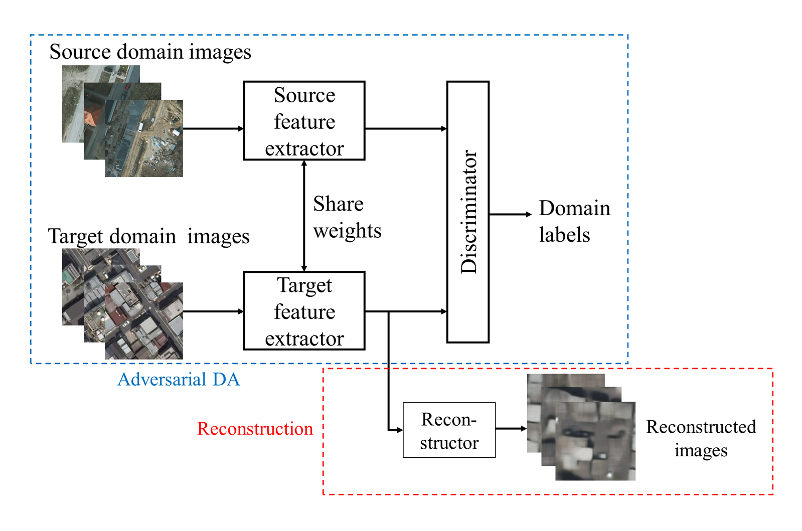
3.1. Vehicle Detection Method

We adopted a region-based object detector for vehicle detection because it is advantageous in terms of both high accuracy and fast computation speed. Specifically, we employed SSD [9] because it has the highest reported accuracy among the well-known region-based detectors, Faster R-CNN, YOLO, and SSD.

The SSD architecture is shown in Figure 1. The network is based on VGG-16, which is a commonly applied architecture proposed by the visual geometry group (VGG) [44]. SSD detects objects based on default boxes that are set at every pixel position in feature maps. Default boxes at one position comprise a square and rectangles of several different aspect ratios, and they are sized according to default box sizes that define the object sizes to be detected. A default box size is determined for each feature map independently. SSD detects objects through convoluting a local 3 × 3 patch at every pixel position of each feature map and predicting object locations expressed by differences from default boxes (offset and scale) and class confidences. In training, default boxes that have overlaps called IoUs (intersection over unions) with bounding boxes of ground truth objects over a specified threshold are regarded as positive examples, and those whose overlaps are under the threshold are regarded as negative examples. We adopted the threshold value of the original paper (0.5), which is a commonly used neutral value.

We set 300 × 300 pixels as the input size. As shown in Figure 1, larger feature maps are used to detect smaller objects, and smaller feature maps are used to detect larger objects. We set 24, 30, 90, 150, 210, 270, and 330 pixels as the default box sizes of each feature map. The default box size of the shallowest feature map is determined to fit the vehicle sizes in the images that we used (0.3 m/pixel resolution). Note that vehicles always appeared in similar sizes in the images, so only the shallowest feature map worked for vehicle detection. SSD originally applies data augmentation techniques to input images to enhance robustness to image condition (e.g., brightness, color space). While the original SSD adopts brightness and color augmentation, random resizing, random cropping, and random horizontal flipping, we applied only brightness and color augmentation. This was because the images that we used in this paper were overhead imagery of the same resolution (see Section 4.1); thus, the other augmentation methods seemed not to be quite effective.

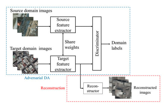
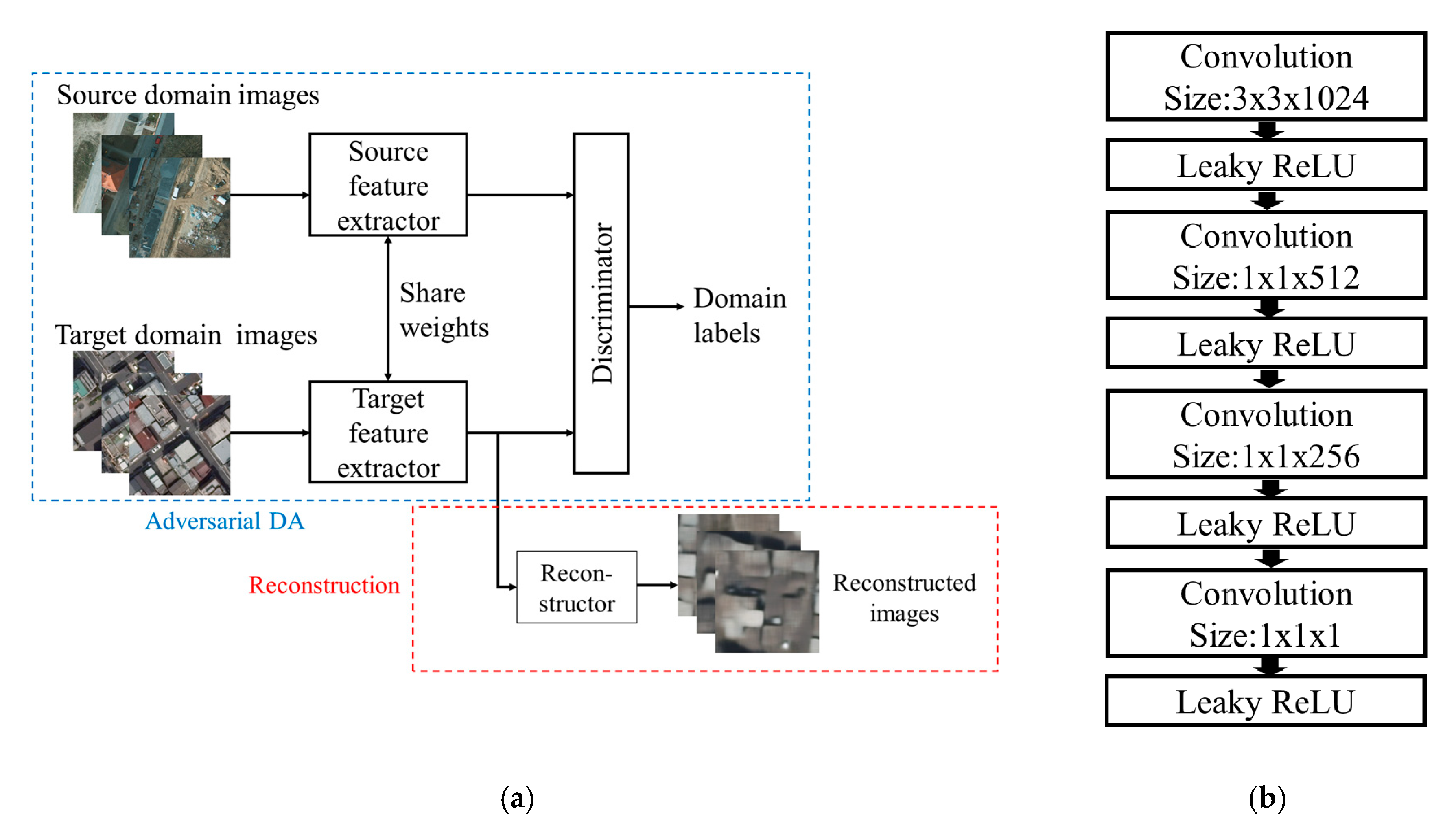
3.2. Domain Adaptation Method

We designed and evaluated two domain adaptation methods: CORAL DA and adversarial DA as baseline methods. We designed CORAL DA based on deep CORAL [31] because it is simple and the original paper reported promising results as compared to other distribution-matching methods. We also designed adversarial DA based on ADDA [34] because ADDA employed effective GAN loss and reported a better result than its competitors.

The overall algorithm of CORAL DA is described in Figure 2.

In CORAL DA, CORAL loss is embedded into a loss function, which is defined as follows:

$$L_{CORAL}=\frac{1}{4d^2}{\parallel C_S-C_T\parallel }_F^2$$

(1)

where ${\parallel ·\parallel }_F^2$ denotes the squared matrix Frobenius norm, d is a dimension of an example, and $C_S$ and $C_F$ are covariance matrices of the source and target examples (extracted features), respectively. Covariance matrices are calculated from examples in each iteration by the following formulations:

$$C_S=\frac{1}{n_S-1}\left(D_S^{\top }{D}_S-\frac{1}{n_S}{\left({\mathbf{1}}^{\top }{D}_S\right)}^{\top }\left({\mathbf{1}}^{\top }{D}_S\right)\right)$$

(2)

$$C_T=\frac{1}{n_T-1}\left(D_T^{\top }{D}_T-\frac{1}{n_T}{\left({\mathbf{1}}^{\top }{D}_T\right)}^{\top }\left({\mathbf{1}}^{\top }{D}_T\right)\right)$$

(3)

where $n_S$ and $n_T$ are numbers of examples of source and target domains, respectively, and $D_S$ and $D_T$ are matrices obtained by stacking examples of the source and target domains, respectively. $\mathbf{1}$ is a column vector whose elements are all one. Each covariance matrix represents a statistic of source or target domain examples; therefore, common features are learned by minimizing the distance of $C_S$ and $C_F$ in each training iteration by calculating $C_S$ from examples in a minibatch, which is the same as $C_F$. This CORAL loss embedded into a loss function is minimized during training, and the features of the source and target domains are aligned.

The overall algorithm of adversarial DA is described in Figure 3a (the rectangle drawn in blue dotted line).

Adversarial DA comprises two adversarial steps. First, a domain discriminator is trained to discriminate features extracted from the source and target domain examples. Conversely, a feature extractor of the target domain is trained to extract features indistinguishable by the discriminator. Training alternates between these adversarial steps and an equilibrium is determined where the features of the source and target domains are aligned. The loss terms of the discriminator ($L_{DIS}$) and the target feature extractor ($L_{EXT}$) are as follows:

$$L_{DIS}=-{\mathbb{E}}_{{\mathrm{x}}_s~{\mathrm{X}}_s}\left[\log D\left(M_s\left({\mathrm{x}}_s\right)\right)\right]-{\mathbb{E}}_{{\mathrm{x}}_t~{\mathrm{X}}_t}\left[\log \left(1-D\left(M_t\left({\mathrm{x}}_t\right)\right)\right)\right]$$

(4)

$$L_{EXT}=-{\mathbb{E}}_{{\mathrm{x}}_t~{\mathrm{X}}_t}\left[\log D\left(M_t\left({\mathrm{x}}_t\right)\right)\right]$$

(5)

where ${\mathrm{X}}_{\mathrm{s}}$ and ${\mathrm{X}}_t$ are examples drawn from the source and target distributions, respectively; D denotes the discriminator; and M represents the feature extractor. Figure 3b shows the discriminator network that we used in this paper. We set the stride and the padding of convolutional filters to one. The discriminator takes a feature map as an input, and we calculated a loss value by aggregating the pixelwise sigmoid cross-entropy of an output of the discriminator. We initialized the source and target feature extractors with a feature extractor of an SSD network pretrained with a vehicle detection dataset. In our adversarial DA, the source and target feature extractors share weights, which means they are the identical network in practice. After the training aligns the source and target feature spaces, classifiers of the SSD network classify features extracted by the target domain feature extractor.

Since deep CORAL and ADDA were originally proposed for image classification networks, we needed to adapt them to the architecture of SSD. In both CORAL and adversarial DA, we regarded the local 3 × 3 patches of a feature map of the SSD network as an independent examples and applied DA methods to those, because the patch is the unit that is fed into the subsequent classifier. In CORAL DA, a patch is serialized into a vector and the CORAL loss was applied to the vector whereas in deep CORAL, the CORAL loss was applied to the output of the last fully connected layer. In adversarial DA, the discriminator just takes a feature map as an input. We applied DA methods only to the 38 × 38 pixel feature map because it was the only feature map that worked in vehicle detection, as mentioned in Section 3.1. In this configuration, the total number of examples in one iteration is 38 × 38 × B, where B is the batchsize. We first pretrained an SSD vehicle detector on a vehicle detection dataset and then trained it by the DA methods, which achieved better performance.

In CORAL DA, we continued vehicle detection training simultaneously with DA training as deep CORAL. The final loss function of CORAL DA is as follows:

$$L_{CORA{L}_{DA}}=L_{SSD}+\alpha L_{CORAL}$$

(6)

where $\alpha$ is a weight coefficient that trades off the adaptation with detection accuracy on the source domain [31].

Although a pretrained model is fine-tuned with only the DA objective in ADDA, we found that the model lost the vehicle detection capability by fine-tuning with only DA objective. Therefore, in adversarial DA, we continued vehicle detection training during the training of the feature extractor in the adversarial steps. The final loss functions of adversarial DA are as follows:

$$\begin{array}{c}{L}_{AD{V}_{DA1}}=L_{DIS} \end{array}$$

(7)

$$\begin{array}{c}{L}_{AD{V}_{DA2}}=L_{SSD}+L_{EXT}\end{array}$$

(8)

where these two objectives are alternated.

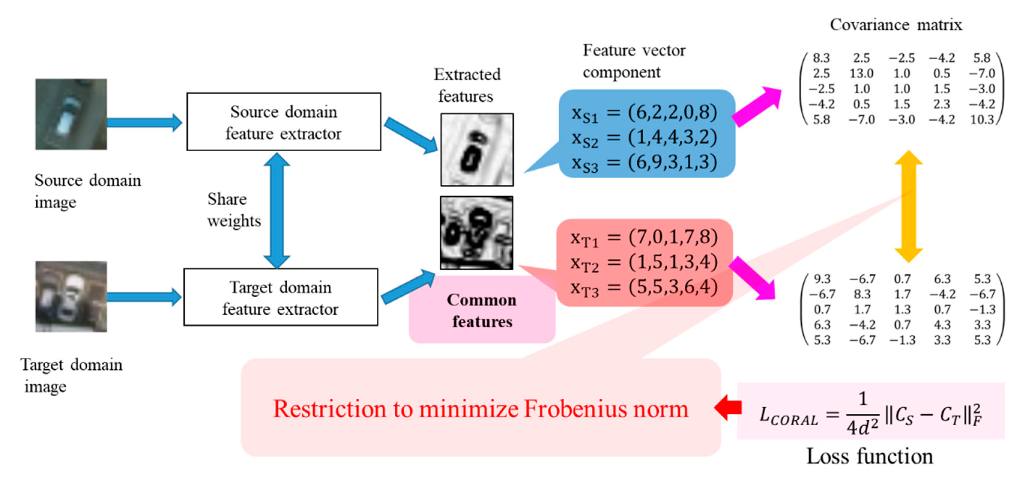
3.3. Reconstruction Loss

Although DA methods can align source and target domain features, there is no explicit objective to learn semantic features in the target domain. Thus, the feature extractor may not learn the semantic features of the target domain sufficiently, and this may lead to performance degradation. To address this drawback, we utilized reconstruction loss. We utilized a reconstructer network to reconstruct an original input image from the feature extracted by the feature extractor. (Figure 3a). The reconstructor and the feature extractor are trained to minimize the mean absolute error between the original input image and the reconstructed image. The reconstruction loss is formulated as follows:

$$L_{REC}={\mathbb{E}}_{{\mathrm{x}}_t~{\mathrm{X}}_t}\left[\frac{1}{w·h·c}\parallel R(M_t\left({\mathrm{x}}_t\right))-{\mathrm{x}}_t\parallel {}_1^{}\right]$$

(9)

where ${\parallel ·\parallel }_1$ denotes the L₁ norm, R represents a reconstructor network, w and h are the width and height of an input image respectively (300 pixels), and c is the channel dimension (3). $L_{REC}$ is added to the training objective of the DA methods. Specifically, in the adversarial DA, $L_{REC}$ is added to Equation (8):

$$\begin{array}{c}{L}_{AD{V}_{DA2}}=L_{SSD}+L_{EXT}+ \gamma L_{REC}\end{array}$$

(10)

where $\gamma$ is a weight coefficient.

As an architecture of the reconstructor network, we adopted the reversed architecture of the feature extractor (VGG-16). For upsampling, we selected the deconvolution layer in place of the unpooling layer for better representation capability. We note that our target of image reconstruction is original source images before applying the data augmentation described in Section 3.1. This is reasonable, because SSD architecture was designed to learn features invariant to such data augmentation for detection robustness. This procedure yielded much faster convergence.

4. Experiments and Results

First, we trained a reference vehicle detector for performance evaluation using the target domain training dataset with annotations in Section 4.3. Next, we trained a detector on an open dataset with vehicle annotations (source domain) and conducted vehicle detection test on the target domain test dataset to demonstrate the performance degradation caused by the domain difference (Section 4.4). Then, we applied DA methods to improve the accuracy and prove their capabilities (Section 4.5 and Section 4.6). As DA methods, we evaluated CORAL DA, adversarial DA, adversarial DA with reconstruction, and a reconstruction only method [45]. Although there were options of combining CORAL DA and Adversarial DA, and CORAL DA with reconstruction, there was no further performance improvement in the preliminary experiments.

Additionally, we tried to further improve the accuracy through utilizing the target domain labeled dataset with the DA methods in Section 4.7.

4.1. Dataset

Although our target of vehicle detection is satellite images, there is no large-scale vehicle detection dataset with annotations of satellite images. Therefore, we utilized the existing vehicle detection dataset by resampling them and simulating experiments on satellite images. We adopted the COWC dataset [21] as a source domain dataset for training a vehicle detector. The COWC dataset is a guaranteed vehicle detection dataset of aerial photos processed by orthorectification and quality vehicle annotations that has been used in many researches. The COWC dataset consists of grayscale and RGB aerial photos processed by orthorectification from six regions containing 32,716 annotated vehicles, excluding large ones such as trucks. The image resolution is 0.15 m/pixel. We only used RGB images from four regions: Toronto, Canada; Selwyn, New Zealand; Potsdam, Germany; and Utah, United States. Figure 4 shows image examples.

Since our target of vehicle detection is satellite images, ground resolution of 0.15 m/pixel is too high. According to the resolution of Worldview3 (0.31 m/pixel), which is one of the highest-resolution commercial satellites, we first downsampled the images to 0.3 m/pixel. Then, we separated the images into a 300 × 300 grid that is the input size of our SSD detection network, selecting every fourth tile as test data and the others as training data. We omitted tiles without vehicles, and duplicated every tile by rotating them by 90, 180, and 270 degrees. These processes yielded the following datasets:

1.

Dataset S_train (Source domain training dataset with annotations)

6264 images of 300 × 300 pixels

2.

Dataset S_test (Source domain test dataset with annotations)

2088 images of 300 × 300 pixels

For the target domain, we used aerial images in Japan. The images are processed by orthorectifications that are the same as the COWC dataset and cover most of the area in the urban Koutou and Sumida wards in Tokyo. The red rectangle in Figure 5a outlines the area where the images were obtained. The resolution is 0.16 m/pixel, and there was no vehicle annotations for the original images.

We once again downsampled the images to 0.3 m/pixel. We separated the areas outlined by the blue rectangles in Figure 5a into a 300 × 300 pixel grid and obtained target domain training images. Then, we randomly extracted 76 images of 1000 × 1000 pixels from the red rectangular area (excluding the blue outlined area). The extracted images had no overlap with each other and the authors carefully annotated these images in the same manner as the COWC dataset. The following datasets were thereby obtained:

3.

Dataset T_train (Target domain training dataset without annotation)

1408 images of 300 × 300 pixels

4.

Dataset T_val (Target domain validation dataset with annotations)

4 images of 1000 × 1000 pixels

5.

Dataset T_test (Target domain test dataset with annotations)

20 images of 1000 × 1000 pixels

6.

Dataset T_labels (Target domain training dataset with annotations)

52 images of 1000 × 1000 pixels

In practice, the image size of satellite images for a vehicle detection test would be relatively large. We set the image size of Dataset T_val, T_test to 1000 pixels, which was determined arbitrarily. (We set the image size of Dataset T_labels to the same 1000 pixels as Dataset T_val and T_test for convenience of annotating process.) Dataset T_labels is processed into images of 300 × 300 pixels when used for training.

All training datasets we used are summarized in

Table 1. Description of all datasets we used in this paper.

Dataset Name	Description	Image Size	Num. of Images	Num. of Vehicles	Purpose	Can Be Seen in:
Dataset S_train	Source domain training dataset with annotations	300 × 300 pixels	6264	93,344	Train all models without TONLY models	Section 4.3, Section 4.4, Section 4.5 and Section 4.7
Dataset S_test	Source domain test dataset with annotations	300 × 300 pixels	2088	31,936	Evaluate performance on source domain	Section 4.4
Dataset T_train	Target domain training dataset without annotation	300 × 300 pixels	1408	-	Train DA models	Section 4.5
Dataset T_val	Target domain validation dataset with annotations	1000 × 1000 pixels	4	834	Check validation accuracy during training to save best snapshot	Section 4.5 and Section 5.3
Dataset T_test	Target domain test dataset with annotations	1000 × 1000 pixels	20	2722	Evaluate performance on target domain	Section 4.3, Section 4.4, Section 4.6 and Section 4.7
Dataset T_labels	Target domain training dataset with annotations	1000 × 1000 pixels	52	5756	Train DA models with labeled dataset	Section 4.3, Section 4.7 and Section 5.4

as a reference.

4.2. Detection Criteria and Accuracy Assessment

While the original SSD detection threshold is an IoU of 0.5, we relaxed it to 0.4 because vehicles in satellite images are very small objects.

When we tested images larger than the SSD input size (300 × 300 pixels), we separated the input images into 300 × 300 pixel tiles, allowing them to overlap with each other by 50 pixels (Figure 6) and conducted vehicle detection in every tile. Then, we aggregated the detection result of every tile and eliminated redundant detections by non-maximum-suppression (NMS) with an IoU threshold of 0.45, which is the same as the original SSD.

To evaluate the vehicle detection performance, we used the following criteria:

• $\mathrm{PR}\left(\mathrm{precision}\mathrm{rate}\right)=\frac{\mathrm{correctly}\mathrm{detected}\mathrm{vehicles}}{\mathrm{detected}\mathrm{vehicles}}$
• $\mathrm{RR}\left(\mathrm{recall}\mathrm{rate}\right)=\frac{\mathrm{correctly}\mathrm{detected}\mathrm{vehicles}}{\mathrm{groundtruth}\mathrm{vehlcles}}$
• $\mathrm{FAR}\left(\mathrm{false}\mathrm{alarm}\mathrm{rate}\right)=\frac{\mathrm{false}\mathrm{detections}}{\mathrm{groundtruth}\mathrm{vehicles}}$
• $\mathrm{F}1(\mathrm{F}1\mathrm{measure})=\frac{2\times \mathrm{PR}\times \mathrm{RR}}{\mathrm{PR}+\mathrm{RR}}$
• $\mathrm{AP}\left(\mathrm{average}\mathrm{precision}\right)$

Average precision (AP) was calculated by checking all detections in descending order of detection confidence and averaging the PR scores when a correct detection appears.

4.3. Reference Accuracy on the Target Domain

First, we trained a reference detector for performance evaluation. For implementation, we customized the SSD implementation of ChainerCV [46] according to the procedure described in Section 3.1. The batchsize was 32, which was the same as in the original paper [9]. We trained the reference detector using Dataset T_labels. Specifically, we started using four images of the target domain training data with annotations and gradually increased the number of images in increments of four. We obtained target domain training patches by separating those 1000 × 1000 pixel images into a 300 × 300 pixel grid and duplicating them by rotating them by 90, 180, and 270 degrees as described in Section 4.1. (Note that the number of training image patches does not increase exactly linearly, because we excluded patches that did not contain a vehicle.) The final number of training patches reached 1564, which was close to the average number of source domain training images per region. We trained two detectors: with Dataset S_train and without Dataset S_train. Training iterations were up to 50,000 with a source domain and up to 20,000 without a source domain (until the loss values converged sufficiently). Figure 7 shows the performance curve on the Dataset T_test. The accuracy seems to have reached near the upper limit when all the target domain training data with annotations were used, and the model trained on both of Dataset S_train and T_labels was slightly better. We use the highest accuracy (78.2% of mean of AP and F1) as a reference score in performance evaluation.

4.4. Detection Performance without DA

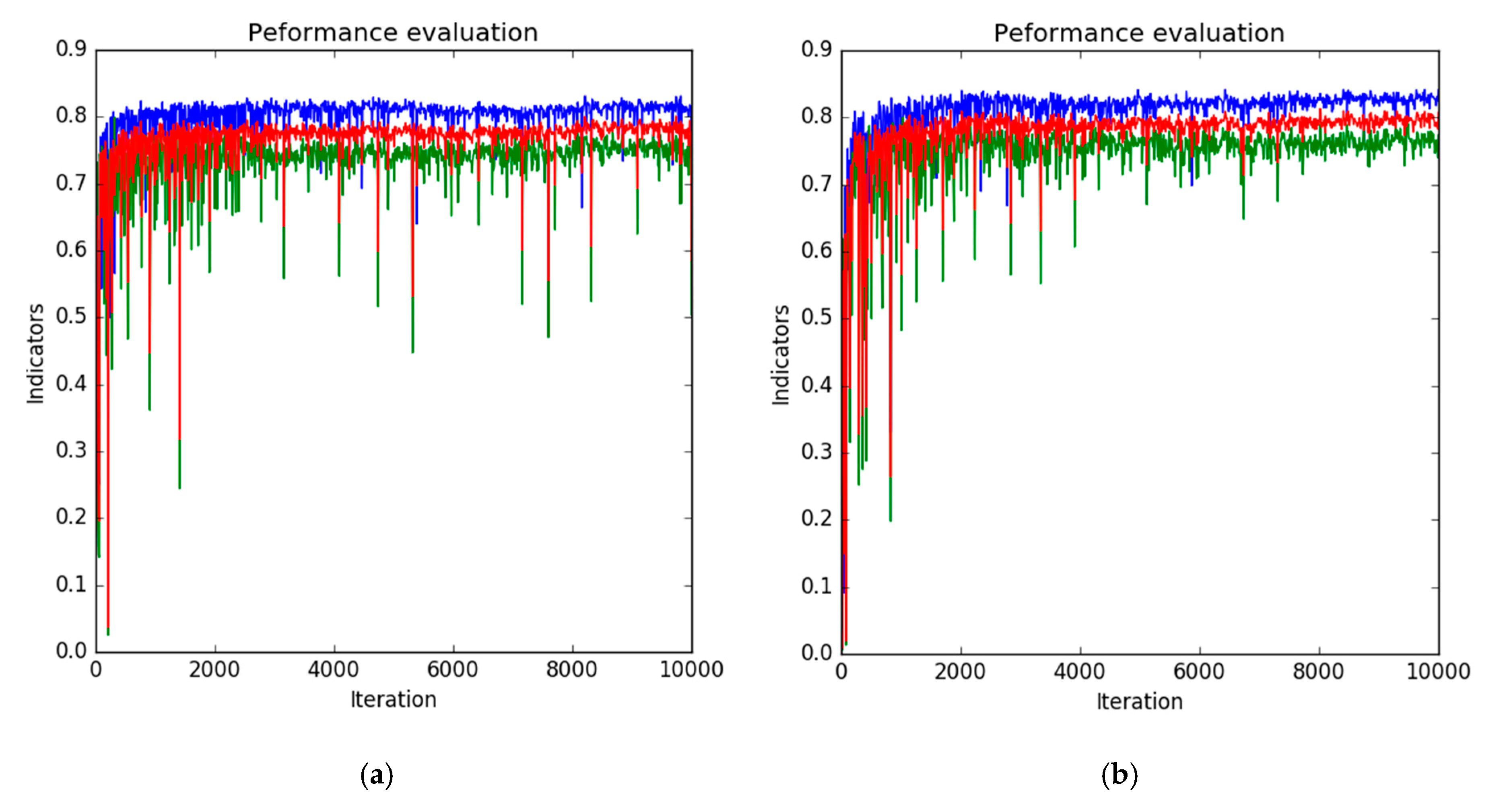
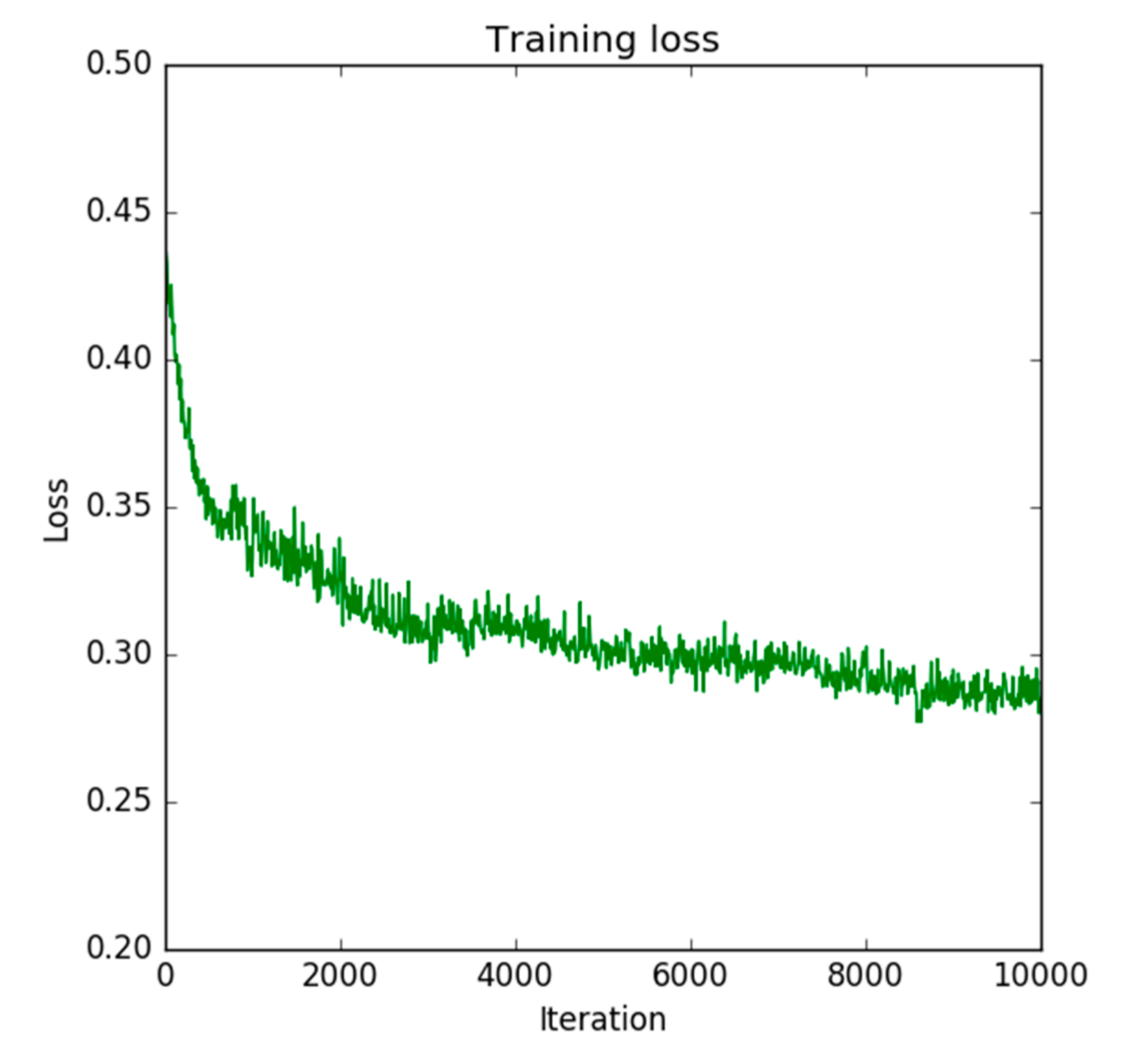
Next, we trained a detector only on the Dataset S_train. The number of training iterations was 40,000, and we changed the schedule of learning rate decay to 28,000 and 35,000 iterations. Figure 8 shows the training curve. Training duration was approximately 18 h on Nvidia Tesla T4. Although there are peaks around 20,000 iterations, it seems to have been caused by random effect because any peak could not be seen in another run. Since the overall trend was stable and training finished successfully, we used the obtained model in the subsequent experiments.

We conducted vehicle detection tests with this trained model on Dataset S_test and Dataset T_test. On Dataset S_test, AP and F1 reached 80.6% and 87.5%, respectively. This is relatively high compared to the reference score in the target domain. This would be because the image features of the target domain (dense area in Tokyo) are complex; thus, the detection in the target domain was more difficult than the source domain. AP and F1 on Dataset T_test were 61.7% and 72.8%. The performance degraded by over 10% from the reference score. Therefore, we applied DA methods to improve on this performance degradation.

For comparison to the state-of-the-art object detection technique, we trained the M2Det [12] detector with Dataset S_train. M2Det employs a multi-level feature pyramid that is advantageous to capture semantic features for detecting small objects and is expected to be robust to domain difference. We selected the VGG-16 backbone, which was the same as our SSD detector for fair comparison. Since the input size of M2Det is 320 pixels, we constructed a training and test dataset in the same manner of constructing the Dataset S_train and S_test where only the image size is changed to 320 pixels. Although M2Det adopt Soft-NMS [47] for high AP, we found that Soft-NMS severely hurt F1 because it never discards any detection of low confidence. Since simply thresholding detections of low confidence did not improve the performance well, we used normal NMS instead of Soft-NMS for fair comparison. The other settings are the same as the original one. Note that the original default box size of M2Det is already suitable to the size of vehicles in our datasets. We utilized the original implementation in pytorch by the authors. Training duration was approximately 14 hours on Nvidia Tesla T4. AP and F1 on Dataset S_test reached 85.4% and 88.6%, respectively. AP and F1 on Dataset T_test were 69.7% and 77.8%. Although the performance much improved in both domains compared to SSD, the margin of improvement in the target domain is much larger than that of the source domain. M2Det showed the expected robustness to domain difference.

4.5. DA Training

We trained the pretrained vehicle detector by DA methods using Dataset S_train and T_train; the batchsize of the continued SSD training remained 32. In CORAL DA, the batchsize was 64, with 32 source domain examples and 32 target domain examples. However, due to the limitation of the capacity of our GPU memory, we calculated CORAL loss from each four examples of source and target domains, which were repeated eight times over a whole batch, and averaged them (4 × 8 = 32 examples in a minibatch of each domain). In the preliminary experiments, $\alpha L_{CORAL}$ tended to a tiny value compared to $L_{SSD}$. Although we tested large coefficient α (e.g., 10) to balance the orders of magnitude of $L_{SSD}$ and $L_{CORAL}$, it did not yield any performance improvement. Thus, we adopt 1 as α. We used an Adam optimizer with parameters $\alpha$, ${\beta }_1$, $\mathrm{and}{\beta }_2$ set at 0.001, 0.9, and 0.999, respectively. The number of training iterations was 25,000.

In adversarial DA, the batchsize was 64, with 32 source domain examples and 32 target domain examples. In the discriminator training, we introduced a buffer [48] that stored the previously extracted feature maps. In one iteration, 32 examples of each domain in a minibatch consisted of 16 examples randomly drawn from the buffer and 16 newly extracted examples that randomly replaced the examples in the buffer. This stabilized the training slightly. The buffer size for each domain was 128. We used an Adam optimizer with parameters $\alpha$, ${\beta }_1$, and ${\beta }_2$ set at 0.0002, 0.0, and 0.9, respectively. The number of training iterations was 15,000.

In adversarial DA with reconstruction, the number of training iterations was 10,000 because the reconstruction objective promoted fast convergence. As for coefficient $\gamma$, we set 0.01 because reconstruction loss (mean absolute error) without $\gamma$ was high (approximately 30) compared to the other loss values and seemed to be a too strong constraint. This was because the reconstructed images remained vague, and images were represented by a 16bit integer in our implementation. The other settings of training were the same as the adversarial DA.

Additionally, we evaluated the reconstruction only method for comparison proposed by [45] as a domain adaptation method. We used the same $\gamma$ as the adversarial DA with reconstruction. The number of training iterations was 10,000.

We evaluated the detection performance of the models on the Dataset T_val every 10 iterations during training to judge the training progress and saved the best snapshots. This was done because it is difficult to judge the training progress only by checking loss values in adversarial training. We used a mean of the AP and F1 scores as the performance indicator of this validation according to the procedure described in Section 4.2.

The training duration of each method was approximately 29 h, 10 h, and 10 h in CORAL DA, adversarial DA, and adversarial DA with reconstruction on two Nvidia Geforce RTX2070 sets. Figure 9 shows the training and validation curves. CORAL loss ($\alpha L_{CORAL}$) became very small in Figure 9a. The discriminator loss ($L_{DIS}$) and extractor loss ($L_{EXT}$) were steady in Figure 9b. Figure 9c shows $\gamma L_{REC}$ in adversarial DA with reconstruction, which remained relatively high after convergence. The reconstruction loss of the reconstruction only method converged smaller than adversarial DA with reconstruction. We omitted the figure of adversarial DA loss values of adversarial DA with reconstruction because it was almost the same as that shown in Figure 9b. In Figure 9d, whereas adversarial DA converged early, CORAL DA took more iterations. Adversarial DA with reconstruction converged further faster than adversarial DA. While the mean values of AP and F1 converged into almost the same value in both CORAL and adversarial DA, adversarial DA with reconstruction remained slightly better. The best scores of mean of AP and F1 for each were 78.4% at iteration 19,590 in CORAL DA, 78.3% at iteration 12,220 in adversarial DA, 78.8% at iteration 9020 in adversarial DA with reconstruction, and 76.5% at iteration 780 in reconstruction only. We saved these snapshots of the SSD model for use in the vehicle detection tests.

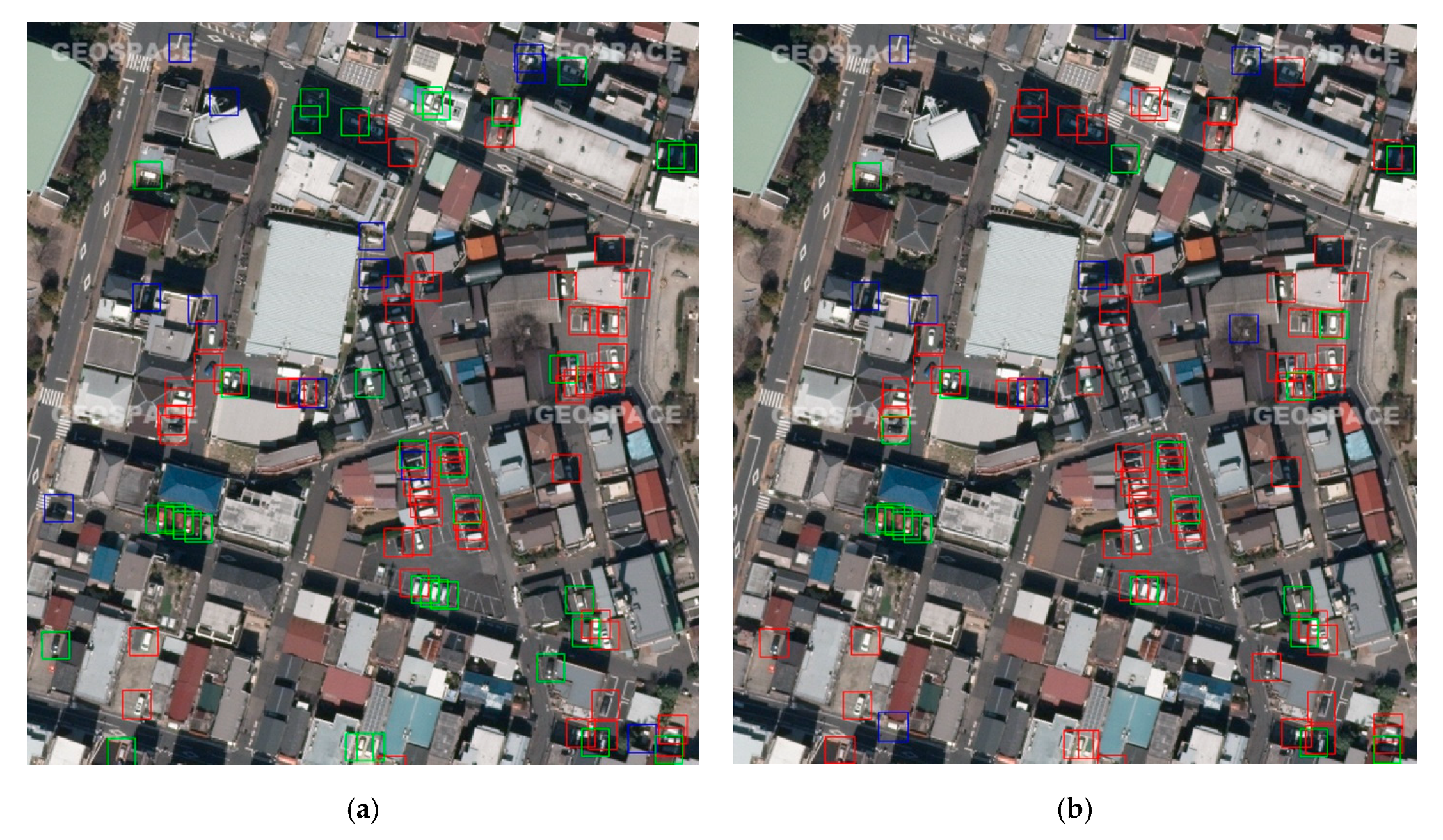
4.6. Detection Performance with DA

Using the above snapshots, we conducted vehicle detection tests on Dataset T_test described in Section 4.1.

Table 2. Detection performance of each method. PR: precision rate, RR: recall rate, FR: false alarm rate.

Method	PR	RR	FAR	AP	F1	Mean of AP and F1
Reference	83.9%	78.5%	15.1%	75.3%	81.1%	78.2%
Without DA	82.6%	65.1%	13.7%	61.7%	72.8%	67.2%
M2Det w/o DA	82.4%	73.7%	15.7%	69.7%	77.8%	73.7%
Reconstruction	81.8%	75.5%	16.8%	72.7%	78.5%	75.6%
CORAL	86.3%	77.1%	12.2%	73.3%	81.5%	77.4%
Adversarial	85.4%	76.5%	13.0%	74.0%	80.7%	77.4%
Adv + Rec	88.0%	77.9%	10.7%	75.2%	82.6%	78.9%

show all of the quantitative scores. All DA methods improved the accuracies. The improvement of RR was relatively larger than that of the others, and it seems to have been the main contributor to the overall performance improvement.

To investigate the effectiveness by reconstruction objective and sensitivity of parameter $\gamma$, we repeated experiments of $\gamma =0, 0.001, 0.01, 0.1$ 10 times. All of the statistics are shown in

Table 3. All statistics of repeated experiments 10 times.

Method	Statistic	PR	RR	FAR	AP	F1	Mean of AP and F1
γ = 0 (w/o rec)	AVR	85.09%	76.52%	13.50%	73.36%	80.55%	76.96%
	STDDEV	2.09%	1.18%	2.42%	0.84%	0.51%	0.45%
	STDERR	0.70%	0.39%	0.81%	0.28%	0.17%	0.15%
γ = 0.001	AVR	85.27%	76.87%	13.34%	73.82%	80.83%	77.32%
	STDDEV	1.79%	1.08%	2.04%	0.91%	0.49%	0.51%
	STDERR	0.60%	0.36%	0.68%	0.30%	0.16%	0.17%
γ = 0.01	AVR	84.37%	77.75%	14.52%	74.78%	80.89%	77.83%
	STDDEV	2.64%	0.93%	3.01%	0.68%	0.98%	0.60%
	STDERR	0.88%	0.31%	1.00%	0.23%	0.33%	0.20%
γ = 0.1	AVR	84.57%	77.26%	14.17%	74.02%	80.72%	77.37%
	STDDEV	2.10%	1.17%	2.42%	0.97%	0.78%	0.72%
	STDERR	0.70%	0.39%	0.81%	0.32%	0.26%	0.24%

and the averages with standard errors are shown in Figure 10.

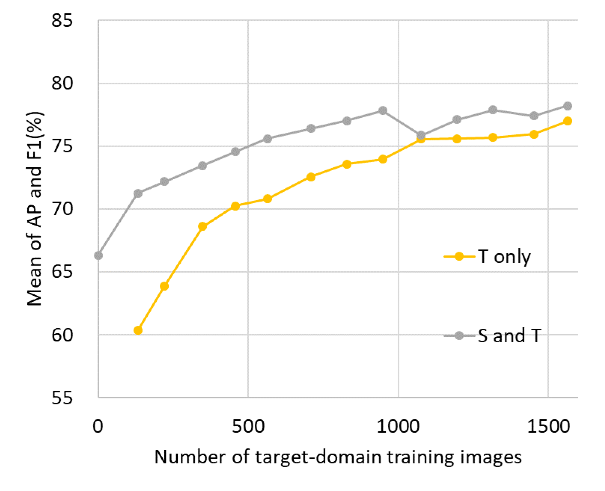
4.7. Utilizing Labeled Dataset with DA Method

We pursued further performance improvement by combining Dataset T_labels with DA methods. We pretrained the SSD model using all of the available labeled dataset (Dataset S_train and T_labels) and fine-tuned it by adversarial DA and adversarial DA with reconstruction. The number of fine-tuning iterations was 10,000. The best validation accuracy (mean of AP and F1) was 80.1% at 9740 iterations in adversarial DA and 81.3% at 8020 iterations in adversarial DA with reconstruction. The performance on Dataset T_test is shown in

Table 4. Detection performance of each method with Dataset T_labels.

Method	PR	RR	FAR	AP	F1	Mean of AP and F1
Adv + target label	87.3%	79.8%	13.0%	77.4%	83.4%	80.4%
Adv + Rec + target label	86.7%	80.4%	12.3%	78.1%	83.4%	80.7%

. Both methods surpassed the reference score explicitly and adversarial DA with reconstruction was slightly better.

5. Discussion

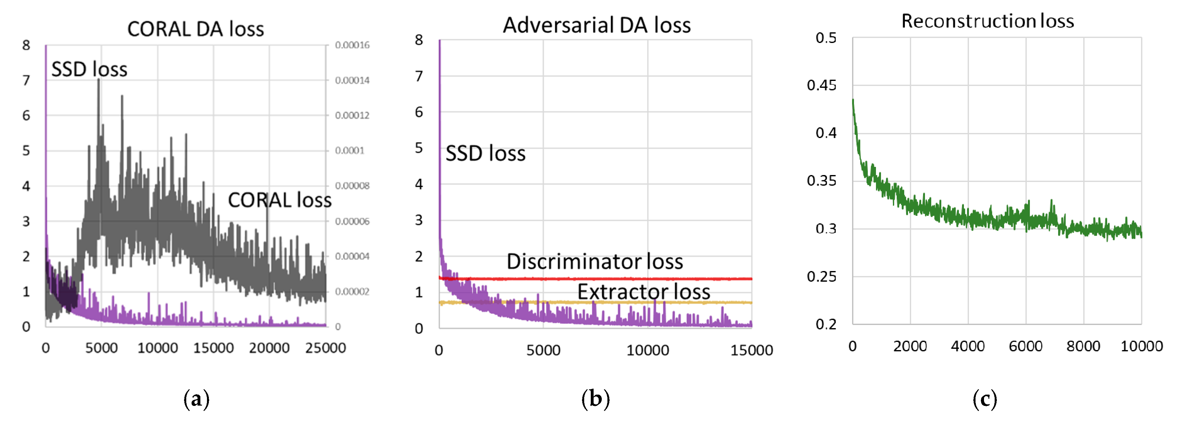
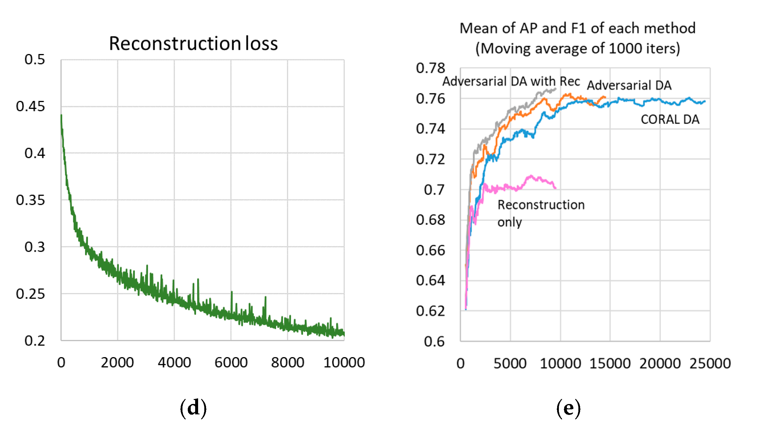
5.1. Performance Improvement by DA

While CORAL DA and adversarial DA significantly improved the accuracy, they were slightly lower than the reference score. In our experiments, CORAL DA and adversarial DA achieved almost the same accuracy, while original ADDA reported better performance than deep CORAL in classification tasks. We assume that this was because the feature differences in the source and target domains in our case were not as significant as other potential DA problems, such as a case of transferring an object detector of RGB images to depth images, and the simple mathematical approach of CORAL DA was enough to generate a high level of accuracy. Meanwhile, the fast convergence adversarial DA is an advantage. Adversarial DA took about 7.5 h for 12,220 iterations, whereas CORAL DA took about 28 h for 19,590 iterations in our implementation. Additionally, adversarial DA still has room for improvement. First, we can enhance the discriminator architecture by adding layers for better representation ability. Second, we can explore other loss functions for adversarial loss. While we adopted conventional sigmoid cross-entropy to calculate adversarial loss, many other loss functions are being studied. One promising candidate is SWD, which is a metric of distance of probability distribution. While it is reported that SWD works well as a metric of distance of image features [39], it seems to be more straightforward to use it to calculate the distance of probability distribution, such as our case of adversarial loss calculation. This will be our future work.

Adversarial DA with reconstruction further improved accuracy that was slightly better than the reference score. Reconstruction loss was not the sole contributor to this performance because the performance of the reconstruction only method was not good (Table 2). Combining reconstruction loss with adversarial DA seems to have effectively worked and facilitated leaning semantic features in the target domain. Further, the reconstruction loss reduced the required iteration number compared to adversarial DA, while calculating the reconstruction objective took additional computational cost in one iteration. Adversarial DA with reconstruction took about 9 h for 9020 iterations, which include a reasonable additional cost (1.5 h) compared to adversarial DA.

Although M2Det surpassed normal SSD by a large margin, especially in the target domain, the result with DA was higher than M2Det. Despite the effectiveness of the ability of a multi-level feature pyramid to efficiently capture semantic features, it seems that a sole multi-level feature pyramid cannot solve the problem of domain difference perfectly and the DA method is still necessary to achieve desirable performance.

Figure 11 shows detection example images. According to the quantitative measures in Table 2, the main contributor of performance improvement by DA is RR improvement. As evidence, while there were many undetected vehicles (green bounding boxes) in Figure 11a, they were significantly reduced and changed to correct detections (red bounding boxes) in Figure 11b.

5.2. Learning Semantic Features by Reconstruction

Figure 12 shows the reconstructed image samples from source and target images by adversarial DA with reconstruction. Even after the training proceeded, the reconstructed images remained vague. This would be because the SSD detection network effectively learned “sparse” features that are only useful for vehicle detection. Compared to the background, vehicles appeared relatively clearly in the reconstructed images. The reconstruction objective worked successfully to learn semantic features, not interfering with the detection task. While the sensitivity of parameter $\gamma$ was not extreme according to Table 3, the best accuracy was obtained at $\gamma =0.01$. We could say that the orders of magnitude of reconstruction loss value should be close to the other loss functions.

Additionally, the image features reconstructed from the source domain resemble the one from the target domain. This is the same phenomenon reported in [45].

According to Figure 10, the improvement margin by reconstruction objective was sufficiently larger than the standard errors. We can say that the reconstruction objective explicitly improved performance. However, the improvement margin was small. This would be because image reconstruction is too simple and redundant as a representation learning method. As discussed above, the SSD learned sparse features useful in object detection. Meanwhile, the reconstruction objective is simple and tries to reconstruct unusable background features. Therefore, the reconstruction objective is not very effective for object detection. Another more effective representation learning method should be explored.

Recently, a new research field called self-supervised learning (SSL) is vigorously studied. In SSL, a pretext task where labels are automatically generated without manual annotation effort is defined and solved to learn semantic features for some task, e.g., image classification or object detection. An example is image inpainting [49]. To reconstruct the missing region of an image, a network needs to be aware of the semantic structure of the image. The network learns semantic features by solving this inpainting task. Another example is predicting the rotation angle of images [50]. An image is rotated by random angles, and a network is trained to predict the angles to learn semantic features. However, those methods are not necessarily effective on satellite images. For example, predicting the rotation angles of overhead imagery seems unreasonable, because the overhead imagery look similar regardless of rotation angles. Although an application of SSL to remote sensing imagery is being studied [51], SSL techniques specific to remote sensing data are still a frontier and should be extensively explored. This will be our future work.

5.3. Reconstruction Objective as Stabilizer

One drawback of the DA method is its instability. Since the DA objective is only to learn target domain features that look similar to source domain features, learnt features can deviate and cause instability. Figure 13a shows the raw validation curve of the method without reconstruction in Section 4.7. Although overall training proceeded successfully, the outlined values appeared frequently in Figure 13a. This is one of the reasons that we adopted the strategy of saving a snapshot that scored the best validation accuracy on Dataset T_val. This instability can be mitigated by a reconstruction objective, as Figure 13b shows, because the reconstruction objective is a conditional, stable objective. A similar effect is reported in [52]. Additionally, we can judge the end of training by checking the trend of reconstruction loss. As Figure 14 shows, reconstruction loss converged at around 10,000 iterations, which was the same as the validation curve in Figure 13b. This would free us from preparing a validation dataset and taking snapshots during training.

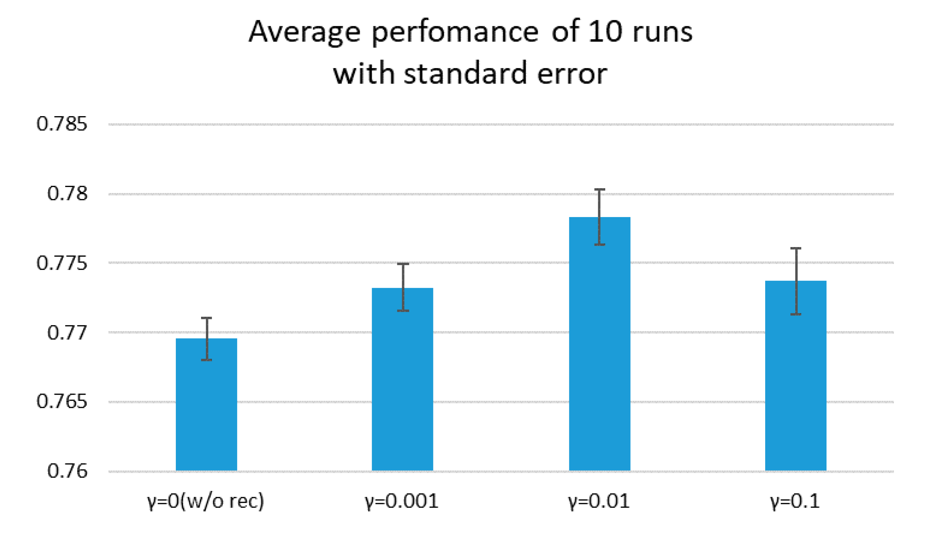
5.4. Effectiveness of Combining Labled Training Data with DA Method

As discussed in Section 4.3, the reference accuracy in the target domain obtained with Dataset T_labels was much lower than the performance in the source domain, because of the image complexity. Even in such a case, it would be possible to achieve higher accuracy by utilizing the DA method, as shown in Section 4.7. The DA method is effective not only in a case where a labeled training dataset is not accessible, but in a case where sufficient labeled dataset cannot achieve desirable high accuracy due to difficulty of target area, such as image feature complexity.

6. Conclusions

We proposed an unsupervised domain adaptation (DA) method to address the performance degradation caused by the image feature differences between the data domains. We tailored the CORAL DA and adversarial DA to our vehicle detector and demonstrated that they significantly improved the detection performance. Further, we introduced reconstruction loss to adversarial DA to facilitate learning semantic features. The reconstruction objective further improved the accuracy and achieved almost the same level of accuracy without any labeled training data than non-DA methods with a sufficient amount of labeled training data of the target domain. The reconstruction objective also stabilized DA training and showed its possibility of simplifying the training procedure. Additionally, we demonstrated that combining the DA method and labeled training dataset can further improve performance. The DA method is effective even in a case where a sufficiently labeled dataset cannot achieve desirable high accuracy due to the difficulty of the target area, such as image feature complexity.

While CORAL DA and adversarial DA achieved almost the same accuracy, adversarial DA has room for improvement. The discriminator architecture could be enhanced by adding layers for better representation ability, and other promising loss functions, e.g., SWD, can be adopted for adversarial loss calculation. Although our reconstruction objective improved the accuracy, the improvement margin was small. This was because reconstruction is too simple as a representation learning method and redundant for object detection tasks. In the context of self-supervised learning, we need to explore a more effective representation learning method suitable to remote-sensing problems. This will be our future work.

References

1. Tang, T.; Zhou, S.; Deng, Z.; Zou, H.; Lei, L. Vehicle Detection in Aerial Images Based on Region Convolutional Neural Networks and Hard Negative Example Mining. Sensors 2017, 17, 336. [Google Scholar] [CrossRef] [PubMed] [Green Version]
2. Gabriela, C. Domain Adaptation for Visual Applications: A Comprehensive Survey. In Domain Adaptation for Visual Applications; Springer: Berlin/Heidelberg, Germany, 2017. [Google Scholar] [CrossRef]
3. Matasci, G.; Volpi, M.; Kanevski, M.; Bruzzone, L.; Tuia, D. Semisupervised Transfer Component Analysis for Domain Adaptation in Remote Sensing Image Classification. IEEE Trans. Geosci. Remote. Sens. 2015, 53, 3550–3564. [Google Scholar] [CrossRef]
4. Girshick, R.; Donahue, J.; Darrell, T.; Malik, J.; Malik, J. Rich Feature Hierarchies for Accurate Object Detection and Semantic Segmentation. In Proceedings of the 2014 IEEE Conference on Computer Vision and Pattern Recognition, Columbus, OH, USA, 23–28 June 2014; pp. 580–587. [Google Scholar]
5. Uijlings, J.R.R.; Van De Sande, K.E.A.; Gevers, T.; Smeulders, A.W.M. Selective Search for Object Recognition. Int. J. Comput. Vis. 2013, 104, 154–171. [Google Scholar] [CrossRef] [Green Version]
6. Girshick, R. Fast R-CNN. In Proceedings of the 2015 IEEE International Conference on Computer Vision (ICCV), Santiago, Chile, 7–13 December 2015; pp. 1440–1448. [Google Scholar]
7. Ren, S.; He, K.; Girshick, R.; Sun, J. Faster R-CNN: Towards real-time object detection with region proposal networks. In Proceedings of the 28th International Conference on Neural Information Processing Systems, Montreal, QC, Canada, 7–12 December 2015; pp. 91–99. [Google Scholar]
8. Redmon, J.; Divvala, S.; Girshick, R.; Farhadi, A. You Only Look Once: Unified, Real-Time Object Detection. In Proceedings of the 2016 IEEE Conference on Computer Vision and Pattern Recognition (CVPR), Las Vegas, NV, USA, 27–30 June 2016; pp. 779–788. [Google Scholar] [CrossRef] [Green Version]
9. Liu, W.; Anguelov, D.; Erhan, D.; Szegedy, C.; Reed, S.; Fu, C.-Y.; Berg, A.C. SSD: Single Shot MultiBox Detector. In Proceedings of the 14th European Conference on Computer Vision (ECCV2016), Amsterdam, The Netherlands, 8–16 October 2016; Volume 9905, pp. 21–37. [Google Scholar] [CrossRef] [Green Version]
10. Lin, T.-Y.; Dollar, P.; Girshick, R.; He, K.; Hariharan, B.; Belongie, S. Feature Pyramid Networks for Object Detection. In Proceedings of the 2017 IEEE Conference on Computer Vision and Pattern Recognition (CVPR2017), Honolulu, HI, USA, 21–26 July 2017; pp. 936–944. [Google Scholar] [CrossRef] [Green Version]
11. Redmon, J.; Farhadi, A. YOLOv3: An Incremental Improvement. arXiv 2018, arXiv:1804.02767. [Google Scholar]
12. Zhao, Q.; Sheng, T.; Wang, Y.; Tang, Z.; Chen, Y.; Cai, L.; Ling, H. M2Det: A Single-Shot Object Detector Based on Multi-Level Feature Pyramid Network. In Proceedings of the AAAI Conference on Artificial Intelligence, Honolulu, Hi, USA, 27 January–1 February 2019; Volume 33, pp. 9259–9266. [Google Scholar] [CrossRef]
13. Chen, X.; Xiang, S.; Liu, C.-L.; Pan, C.-H. Vehicle Detection in Satellite Images by Hybrid Deep Convolutional Neural Networks. IEEE Geosci. Remote Sens. Lett. 2014, 11, 1797–1801. [Google Scholar] [CrossRef]
14. Qu, S.; Wang, Y.; Meng, G.; Pan, C. Vehicle Detection in Satellite Images by Incorporating Objectness and Convolutional Neural Network. J. Ind. Intell. Inf. 2016, 4, 158–162. [Google Scholar] [CrossRef]
15. Cheng, M.-M.; Zhang, Z.; Lin, W.-Y.; Torr, P. BING: Binarized Normed Gradients for Objectness Estimation at 300fps. In Proceedings of the 2014 IEEE Conference on Computer Vision and Pattern Recognition (CVPR), Columbus, OH, USA, 23–28 June 2014; pp. 3286–3293. [Google Scholar] [CrossRef] [Green Version]
16. Schapire, R.E.; Singer, Y. Improved Boosting Algorithms Using Confidence-rated Predictions. Mach. Learn. 1999, 37, 297–336. [Google Scholar] [CrossRef] [Green Version]
17. Car Localization and Counting with Overhead Imagery, an Interactive Exploration. Available online: https://medium.com/the-downlinq/car-localization-and-counting-with-overhead-imagery-an-interactive-exploration-9d5a029a596b (accessed on 29 December 2019).
18. Mundhenk, T.N.; Konjevod, G.; Sakla, W.A.; Boakye, K. A Large Contextual Dataset for Classification, Detection and Counting of Cars with Deep Learning. In Proceedings of the 14th European Conference on Computer Vision (ECCV2016), Amsterdam, The Netherlands, 8–16 October 2016; Volume 9907, pp. 785–800. [Google Scholar] [CrossRef] [Green Version]
19. Szegedy, C.; Liu, W.; Jia, Y.; Sermanet, P.; Reed, S.; Anguelov, D.; Erhan, D.; Vanhoucke, V.; Rabinovich, A. Going deeper with convolutions. In Proceedings of the 2015 IEEE Conference on Computer Vision and Pattern Recognition (CVPR), Boston, MA, USA, 7–12 June 2015; pp. 1–9. [Google Scholar] [CrossRef] [Green Version]
20. He, K.; Zhang, X.; Ren, S.; Sun, J. Deep Residual Learning for Image Recognition. In Proceedings of the 2016 IEEE Conference on Computer Vision and Pattern Recognition (CVPR), Las Vegas, NV, USA, 27–30 June 2016; pp. 770–778. [Google Scholar] [CrossRef] [Green Version]
21. Cars Overhead With Context. Available online: https://gdo152.llnl.gov/cowc/ (accessed on 29 December 2019).
22. Zheng, K.; Wei, M.; Sun, G.; Anas, B.; Li, Y. Using Vehicle Synthesis Generative Adversarial Networks to Improve Vehicle Detection in Remote Sensing Images. ISPRS Int. J. Geo-Inf. 2019, 8, 390. [Google Scholar] [CrossRef] [Green Version]
23. Zhang, X.; Zhu, X. An Efficient and Scene-Adaptive Algorithm for Vehicle Detection in Aerial Images Using an Improved YOLOv3 Framework. ISPRS Int. J. Geo-Inf. 2019, 8, 483. [Google Scholar] [CrossRef] [Green Version]
24. Bovik, A. Handbook of Image and Video Processing, 2nd ed.; A volume in Communications, Networking and Multimedia; Academic Press: Orlando, FL, USA, 2005. [Google Scholar]
25. Kwan, C.; Hagen, L.; Chou, B.; Perez, D.; Li, J.; Shen, Y.; Koperski, K. Simple and effective cloud- and shadow-detection algorithms for Landsat and Worldview images. Signal Image Video Process. 2019, 14, 125–133. [Google Scholar] [CrossRef]
26. Shorten, C.; Khoshgoftaar, T.M. A survey on Image Data Augmentation for Deep Learning. J. Big Data 2019, 6, 60. [Google Scholar] [CrossRef]
27. Borgwardt, K.M.; Gretton, A.; Rasch, M.J.; Kriegel, H.-P.; Schölkopf, B.; Smola, A.J. Integrating structured biological data by Kernel Maximum Mean Discrepancy. Bioinformatics 2006, 22, 49–57. [Google Scholar] [CrossRef] [PubMed] [Green Version]
28. Sun, B.; Feng, J.; Saenko, K. Return of frustratingly easy domain adaptation. In Proceedings of the Thirtieth AAAI Conference on Artificial Intelligence (AAAI-16), Phoenix, AZ, USA, 12–17 February 2016; pp. 2058–2065. [Google Scholar]
29. Tzeng, E.; Hoffman, J.; Zhang, N.; Saenko, K.; Darrell, T. Deep domain confusion: Maximizing for domain invariance. arXiv 2014, arXiv:1412.3474. [Google Scholar]
30. Long, M.; Cao, Y.; Wang, J.; Jordan, M.I. Learning transferable features with deep adaptation networks. In Proceedings of the 32nd International Conference on Machine Learning (ICML 2015), Lille, France, 6–11 July 2015; Volume 37, pp. 97–105. [Google Scholar]
31. Sun, B.; Saenko, K. Deep CORAL: Correlation Alignment for Deep Domain Adaptation. In Proceedings of the 14th European Conference on Computer Vision (ECCV2016), Amsterdam, The Netherlands, 8–16 October 2016; pp. 443–450. [Google Scholar] [CrossRef] [Green Version]
32. Tzeng, E.; Hoffman, J.; Darrell, T.; Saenko, K. Simultaneous Deep Transfer across Domains and Tasks. In Proceedings of the 2015 IEEE International Conference on Computer Vision (ICCV2015), Santiago, Chile, 11–18 December 2015; pp. 4068–4076. [Google Scholar]
33. Ganin, Y.; Ustinova, E.; Ajakan, H.; Germain, P.; Larochelle, H.; Laviolette, F.; Marchand, M.; Lempitsky, V. Domain adversarial training of neural networks. J. Mach. Learn. Res. 2016, 17, 1–35. [Google Scholar]
34. Tzeng, E.; Hoffman, J.; Saenko, K.; Darrell, T. Adversarial Discriminative Domain Adaptation. In Proceedings of the 2017 IEEE Conference on Computer Vision and Pattern Recognition (CVPR2017), Honolulu, HI, USA, 21–26 July 2017; pp. 2962–2971. [Google Scholar] [CrossRef] [Green Version]
35. Goodfellow, I.; Pouget-Abadie, J.; Mirza, M.; Xu, B.; Warde-Farley, D.; Ozair, S.; Courville, A.; Bengio, Y. Generative adversarial nets. In Proceedings of the Advances in Neural Information Processing Systems 27 (NIPS2014), Montréal, QC, Canada, 8–13 December 2014; pp. 2672–2680. [Google Scholar]
36. Pan, S.J.; Tsang, I.; Kwok, J.T.; Yang, Q. Domain adaptation via transfer component analysis. IEEE Trans. Neural Netw. Feb. 2011, 22, 199–210. [Google Scholar] [CrossRef] [PubMed] [Green Version]
37. Garea, A.S.S.; Heras, D.B.; Argüello, F. TCANet for Domain Adaptation of Hyperspectral Images. Remote Sens. 2019, 11, 2289. [Google Scholar] [CrossRef] [Green Version]
38. Bejiga, M.B.; Melgani, F.; Beraldini, P. Domain Adversarial Neural Networks for Large-Scale Land Cover Classification. Remote Sens. 2019, 11, 1153. [Google Scholar] [CrossRef] [Green Version]
39. Rostami, M.; Kolouri, S.; Eaton, E.; Kim, K. Deep Transfer Learning for Few-Shot SAR Image Classification. Remote Sens. 2019, 11, 1374. [Google Scholar] [CrossRef] [Green Version]
40. Rabin, J.; Peyré, G.; Delon, J.; Bernot, M. Wasserstein barycenter and its application to texture mixing. In International Conference on Scale Space and Variational Methods in Computer Vision; Springer: Berlin/Heidelberg, Germany, 2011; pp. 435–446. [Google Scholar]
41. Benjdira, B.; Bazi, Y.; Koubaa, A.; Ouni, K. Unsupervised Domain Adaptation Using Generative Adversarial Networks for Semantic Segmentation of Aerial Images. Remote Sens. 2019, 11, 1369. [Google Scholar] [CrossRef] [Green Version]
42. Zhu, J.-Y.; Park, T.; Isola, P.; Efros, A.A. Unpaired Image-to-Image Translation Using Cycle-Consistent Adversarial Networks. In Proceedings of the 2017 IEEE International Conference on Computer Vision (ICCV), Venice, Italy, 22–29 October 2017; pp. 2242–2251. [Google Scholar] [CrossRef] [Green Version]
43. Hoffman, J.; Tzeng, E.; Park, T.; Zhu, J.; Isola, P.; Saenko, K.; Efros, A.; Darrell, T. CyCADA: Cycle-Consistent Adversarial Domain Adaptation. In Proceedings of the 35th International Conference on Machine Learning, Stockholm, Sweden, 10–15 July 2018; Volume 80, pp. 1989–1998. [Google Scholar]
44. Simonyan, K.; Zisserman, A. Very Deep Convolutional Networks for Large-Scale Image Recognition. arXiv 2014, arXiv:1409.1556. [Google Scholar]
45. Ghifary, M.; Kleijn, W.B.; Zhang, M.; Balduzzi, D.; Li, W. Deep Reconstruction-Classification Networks for Unsupervised Domain Adaptation. In Proceedings of the 14th European Conference on Computer Vision (ECCV2016), Amsterdam, The Netherlands, 8–16 October 2016; Volume 9908, pp. 597–613. [Google Scholar] [CrossRef] [Green Version]
46. Niitani, Y.; Ogawa, T.; Saito, S.; Saito, M. ChainerCV: A Library for Deep Learning in Computer Vision. In Proceedings of the ACM Multimedia Conference, Mountain View, CA, USA, 23–27 October 2017; pp. 1217–1220. [Google Scholar] [CrossRef]
47. Bodla, N.; Singh, B.; Chellappa, R.; Davis, L.S. Soft-NMS—Improving Object Detection with One Line of Code. In Proceedings of the 2017 IEEE International Conference on Computer Vision (ICCV), Venice, Italy, 22–29 October 2017; pp. 5562–5570. [Google Scholar] [CrossRef] [Green Version]
48. Shrivastava, A.; Pfister, T.; Tuzel, O.; Susskind, J.; Wang, W.; Webb, R. Learning from Simulated and Unsupervised Images through Adversarial Training. In Proceedings of the 2017 IEEE Conference on Computer Vision and Pattern Recognition (CVPR2017), Honolulu, HI, USA, 21–26 July 2017; pp. 2242–2251. [Google Scholar] [CrossRef] [Green Version]
49. Pathak, D.; Krahenbuhl, P.; Donahue, J.; Darrell, T.; Efros, A.A. Context Encoders: Feature Learning by Inpainting. In Proceedings of the 2016 IEEE Conference on Computer Vision and Pattern Recognition (CVPR), Las Vegas, NV, USA, 26 June–1 July 2016; pp. 2536–2544. [Google Scholar]
50. Gidaris, S.; Singh, P.; Komodakis, N. Unsupervised Representation Learning by Predicting Image Rotations. In Proceedings of the 6th International Conference on Learning Representations (ICLR2018), Vancouver, BC, Canada, 30 April–3 May 2018. [Google Scholar]
51. Singh, S.; Batra, A.; Pang, G.; Torresani, L.; Basu, S.; Paluri, M.; Jawahar, C.V. Self-Supervised Feature Learning for Semantic Segmentation of Overhead Imagery. In Proceedings of the 29th British Machine Vision Conference (BMVC2018), Newcastle, UK, 3–6 September 2018. [Google Scholar]
52. Chen, T.; Zhai, X.; Ritter, M.; Lucic, M.; Houlsby, N. Self-Supervised GANs via Auxiliary Rotation Loss. In Proceedings of the 2019 IEEE/CVF Conference on Computer Vision and Pattern Recognition (CVPR), Long Beach, CA, USA, 15–20 June 2019; pp. 12146–12155. [Google Scholar] [CrossRef] [Green Version]
Figure 1. Single Shot Multibox Detector (SSD) architecture.
Remotesensing 12 00575 g001
Figure 2. Overview of Correlation alignment (CORAL) domain adaptation (DA).
Remotesensing 12 00575 g002
Figure 3. Overview of adversarial DA: (a) algorithm and (b) discriminator network. Leaky ReLU is a variant of the activation function called rectified linear unit (ReLU).
Remotesensing 12 00575 g003
Figure 4. Image examples from the four study regions from the Cars Overhead with Context (COWC) dataset: (a) Toronto, Canada; (b) Selwyn, New Zealand; (c) Potsdam, Germany; and (d) Utah, United States.
Remotesensing 12 00575 g004
Figure 5. Study area in Japan. (a) Map of Tokyo. The red rectangle outlines the study area for which aerial images were obtained. We extracted non-labeled training images for DA from the area outlined by the blue rectangles and labeled training and test images from the area outlined by the red rectangle (excluding the blue rectangles) where the latter images were manually annotated. (b) An example image.
Remotesensing 12 00575 g005
Figure 6. Detection procedure for an image larger than 300 × 300 pixels. The image is separated into 300 × 300 pixel tiles with an overlap of 50 pixels, and the detection results of each tile are merged.
Remotesensing 12 00575 g006
Figure 7. Detection accuracy improvement in each condition by increment of labeled training data of the target domain. S and T represent the source and target domains, respectively.
Remotesensing 12 00575 g007
Figure 8. SSD training curve with the Dataset S_train. “Loss” represents L S S D , which is the sum of the localization loss (“loss/loc”) and the classification loss (“loss/conf”).
Remotesensing 12 00575 g008
Figure 9. Training and validation curves of each DA method: (a) CORAL DA loss, (b) adversarial DA loss, (c) reconstruction loss in Adversarial DA with reconstruction, (d) reconstruction loss in the reconstruction-only method, (e) validation accuracy (1000 iterations moving average of mean of average precision (AP) and F1 measure (F1)) of each DA method. Best viewed in color. The black, purple, yellow, red, green, gray, orange, blue, and pink lines represent CORAL loss, SSD loss, extractor loss, discriminator loss, reconstruction loss, scores of mean of AP and F1 in adversarial DA with reconstruction, adversarial DA, CORAL DA, and reconstruction only, respectively.
Remotesensing 12 00575 g009aRemotesensing 12 00575 g009b
Figure 10. Average scores with various γ .
Remotesensing 12 00575 g010
Figure 11. Examples of detection results: (a) before applying DA and (b) after applying Adv with rec. The red, blue, and green bounding boxes represent true positives (correct detections), false positives (misdetections), and false negatives (undetected groundtruth vehicles), respectively.
Remotesensing 12 00575 g011
Figure 12. Reconstructed image samples. (a) An original source domain image, (b) a reconstructed source domain image, (c) an original target domain image, (d) a reconstructed target domain image.
Remotesensing 12 00575 g012aRemotesensing 12 00575 g012b
Figure 13. Validation curve of methods in Section 4.7: (a) without reconstruction, (b) with reconstruction. Blue, green, and red lines represent F1, AP, and mean of F1 and AP, respectively.
Remotesensing 12 00575 g013
Figure 14. The curve of reconstruction loss in the method with reconstruction in Section 4.7.
Remotesensing 12 00575 g014