Spatio-Temporal Mapping of Multi-Satellite Observed Column Atmospheric CO2 Using Precision-Weighted Kriging Method

 and
and
Abstract
:
1. Introduction
2. Dataset
2.1. XCO2 from Multi-Satellite Observations
2.2. The Total Carbon Column Observing Network
2.3. XCO2 from Model Simulation
3. Method
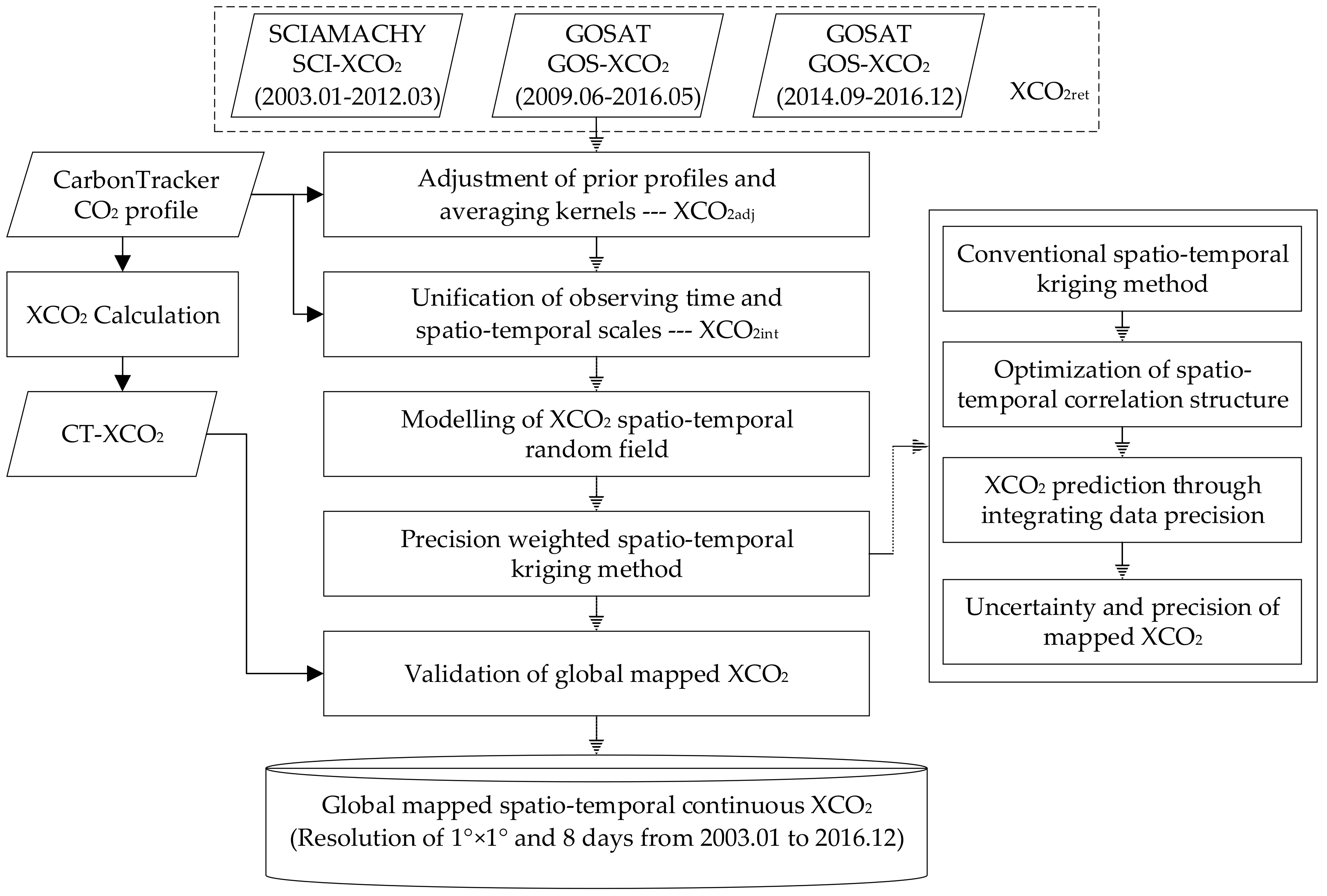
3.1. Preprocessing
3.1.1. Adjustment of a Priori Vertical Profiles and Averaging Kernels
3.1.2. Unification of Observing Time and Spatio-Temporal Scales
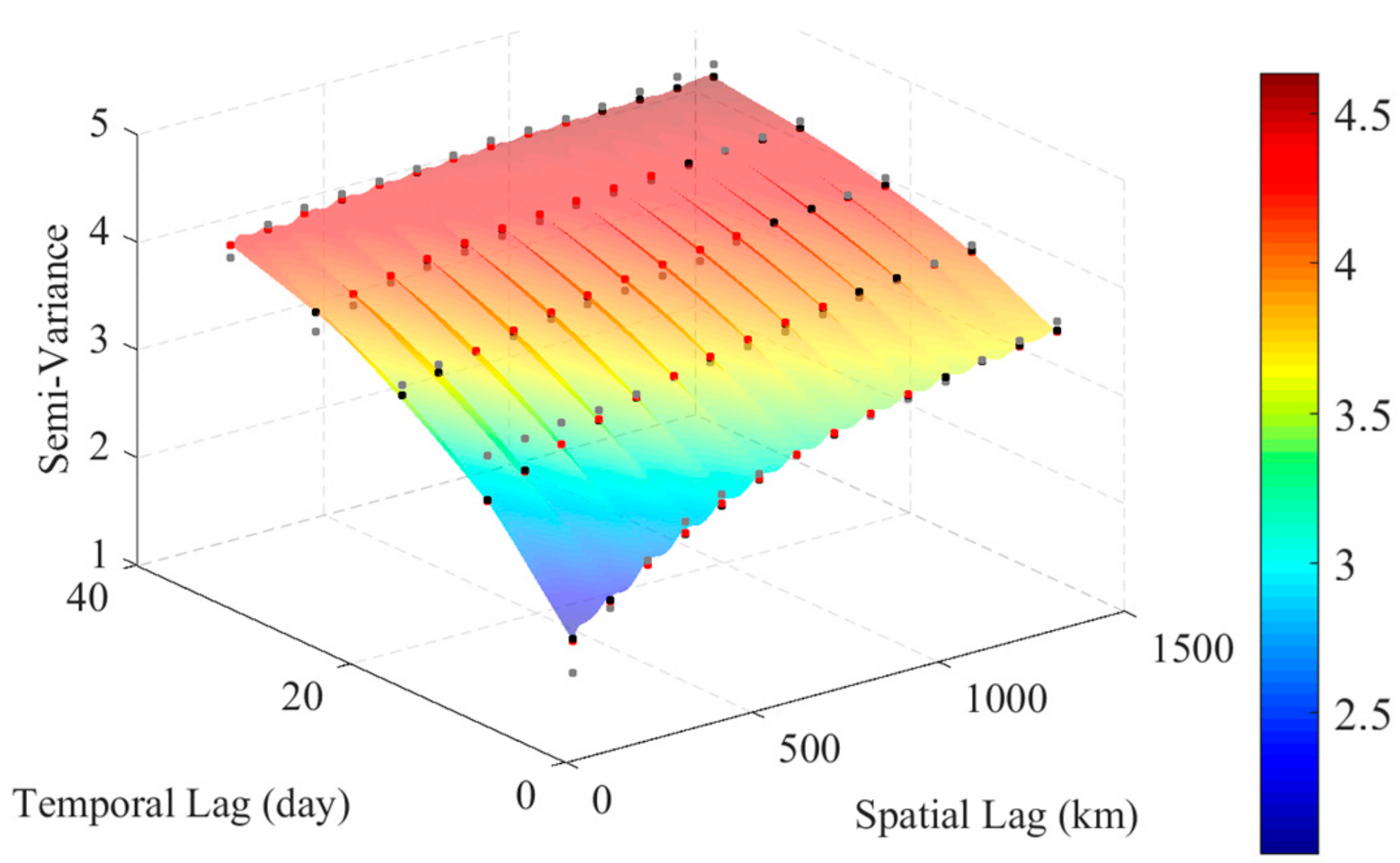
3.2. Modeling XCO2 Spatio-Temporal Random Field for use in Kriging
3.3. Precision Weighted Spatio-Temporal Kriging
3.3.1. Conventional Spatio-Temporal Kriging
3.3.2. Optimization of Spatio-Temporal Correlation Structure
3.3.3. Integrating XCO2 Using Variable Data Precision
3.3.4. Uncertainty and Precision of Mapped XCO2
3.4. Validation of Global Mapped XCO2
4. Results
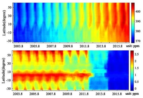
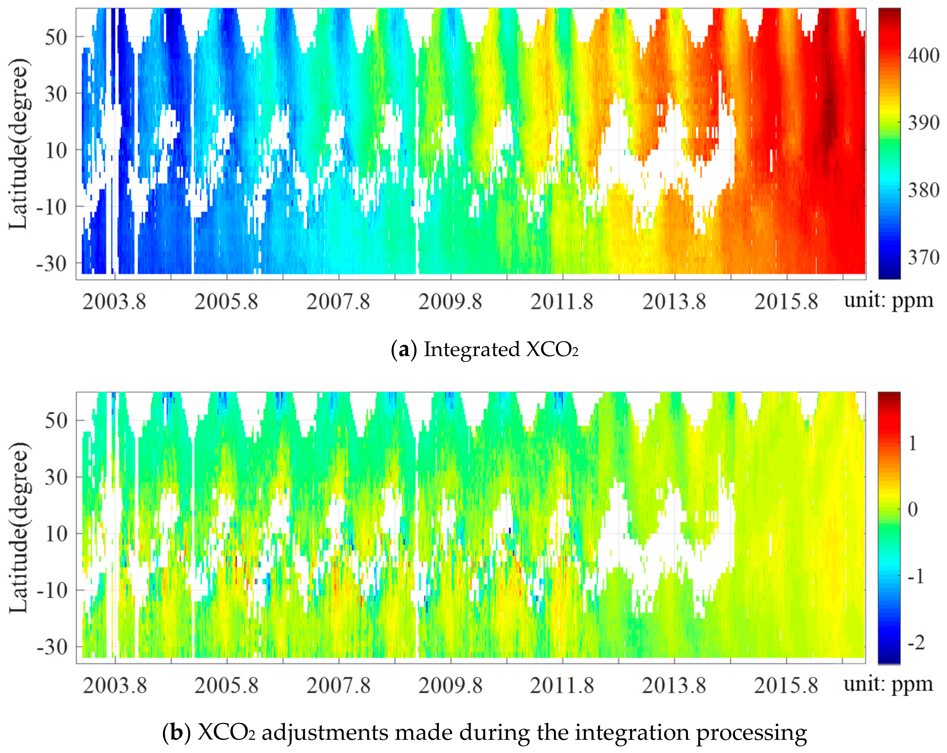
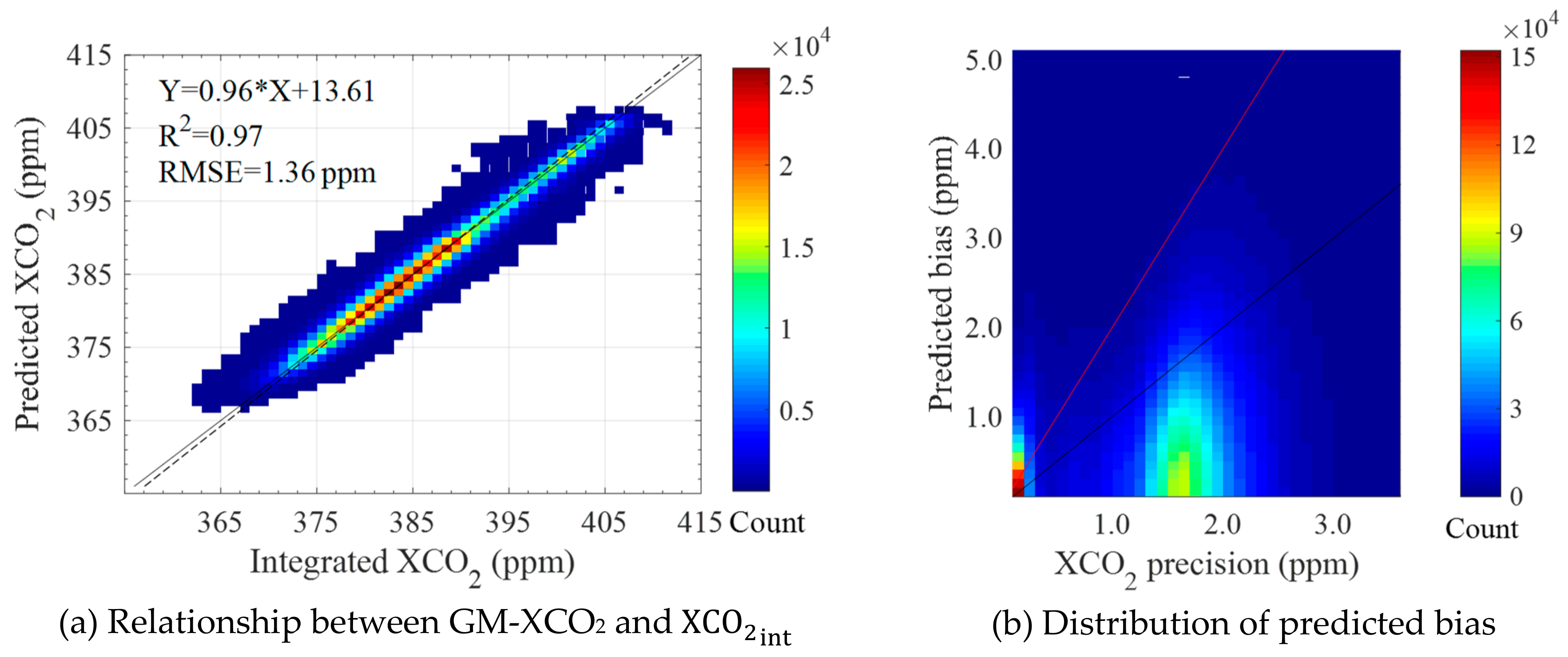
4.1. Integrated-XCO2 from Three Satellites
4.2. Globally-Mapped XCO2
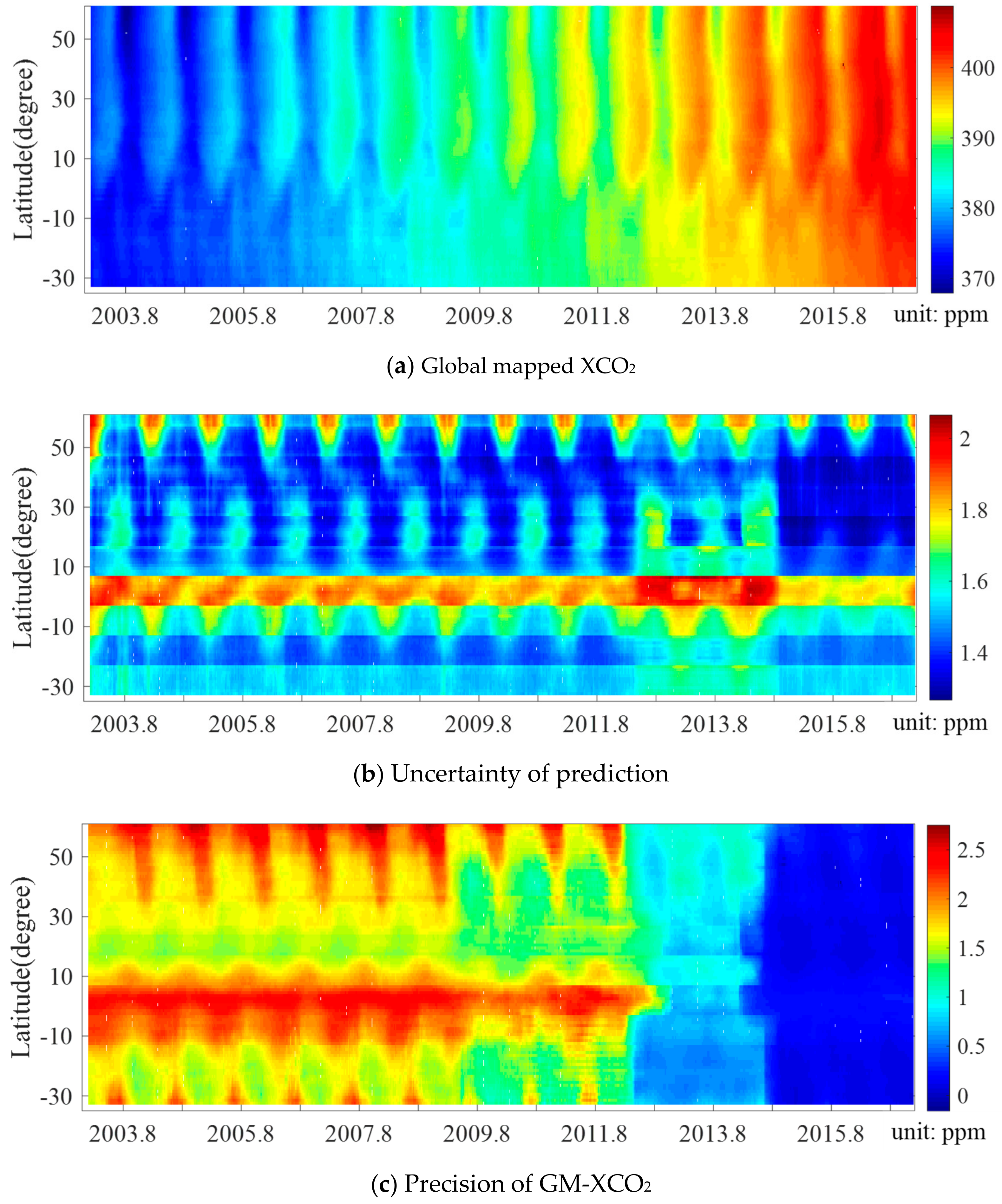
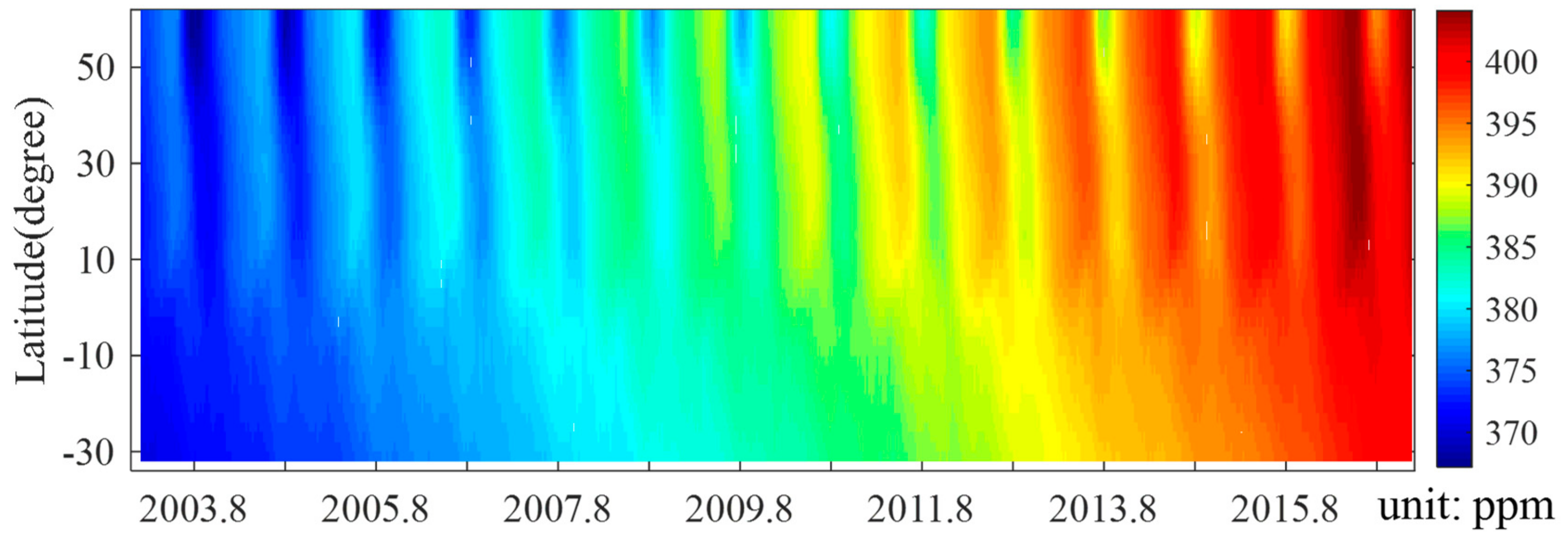
4.2.1. Latitudinal and Temporal Variability of Globally Mapped XCO2
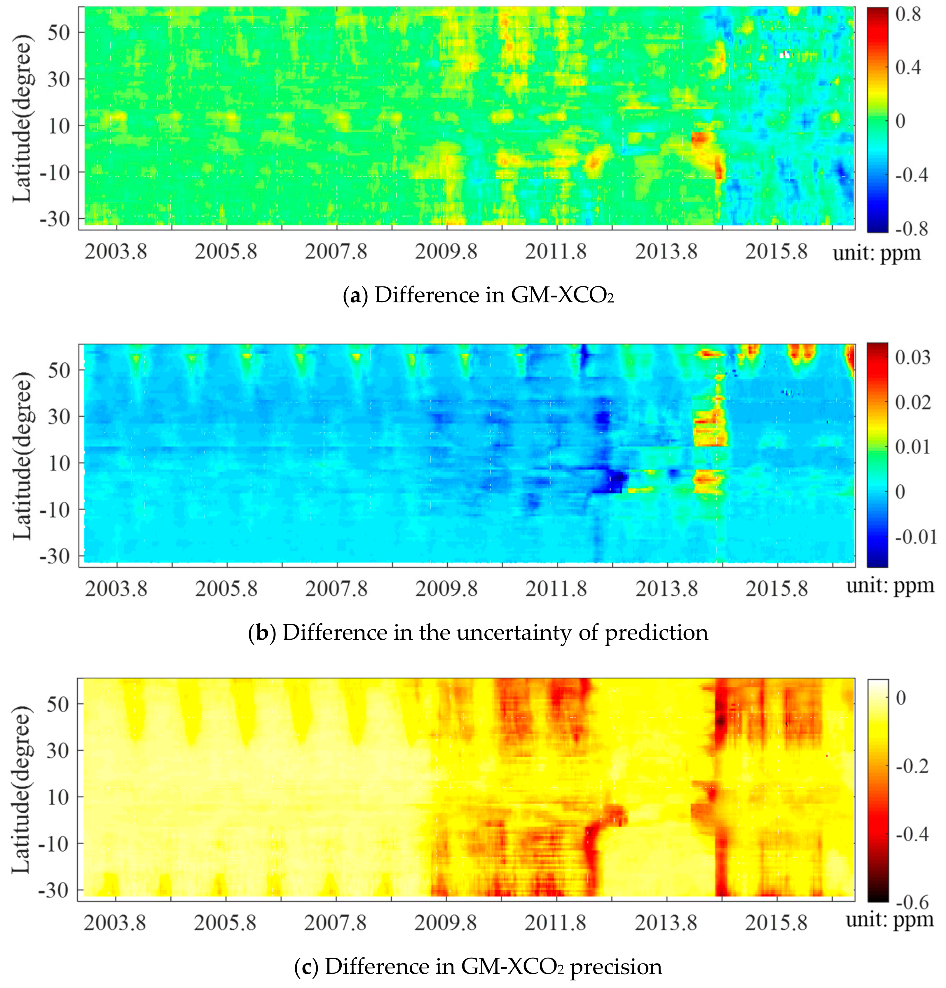
4.2.2. Comparison with Conventional Spatio-Temporal Kriging Results
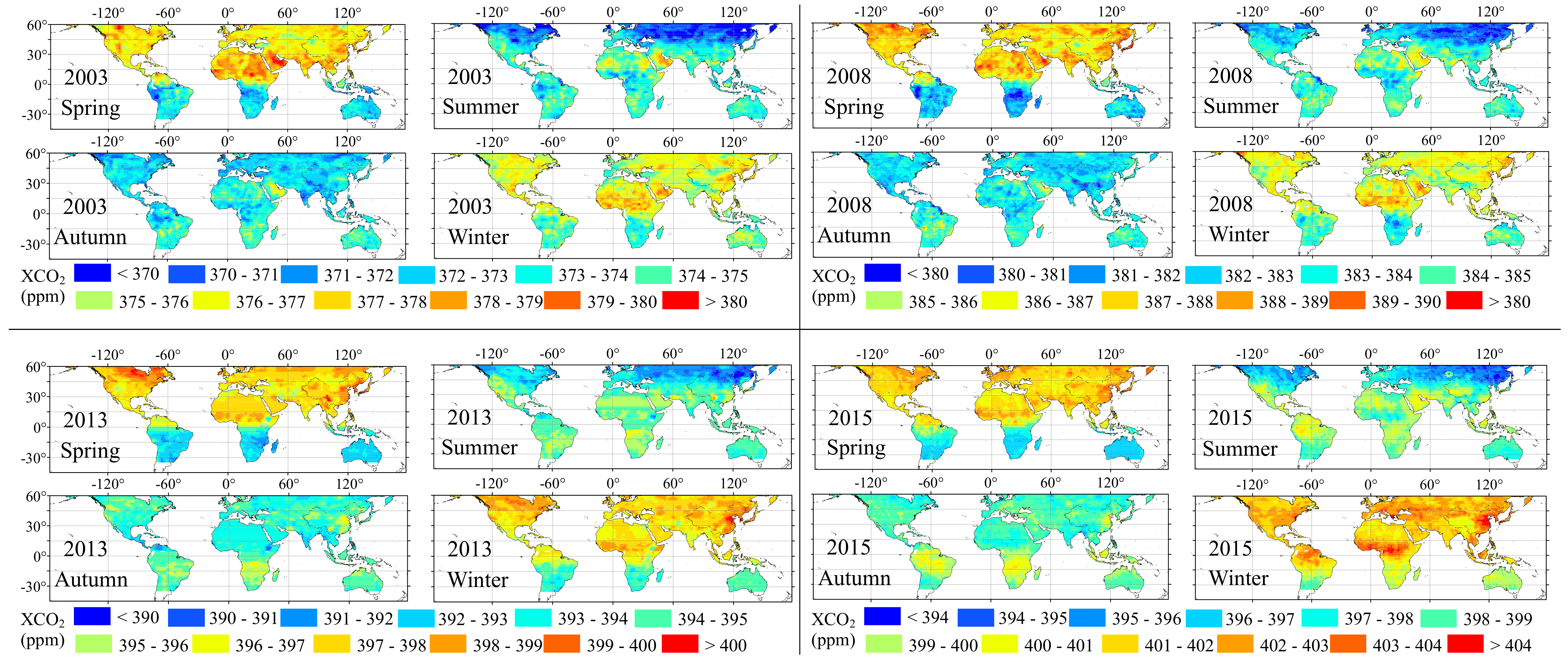
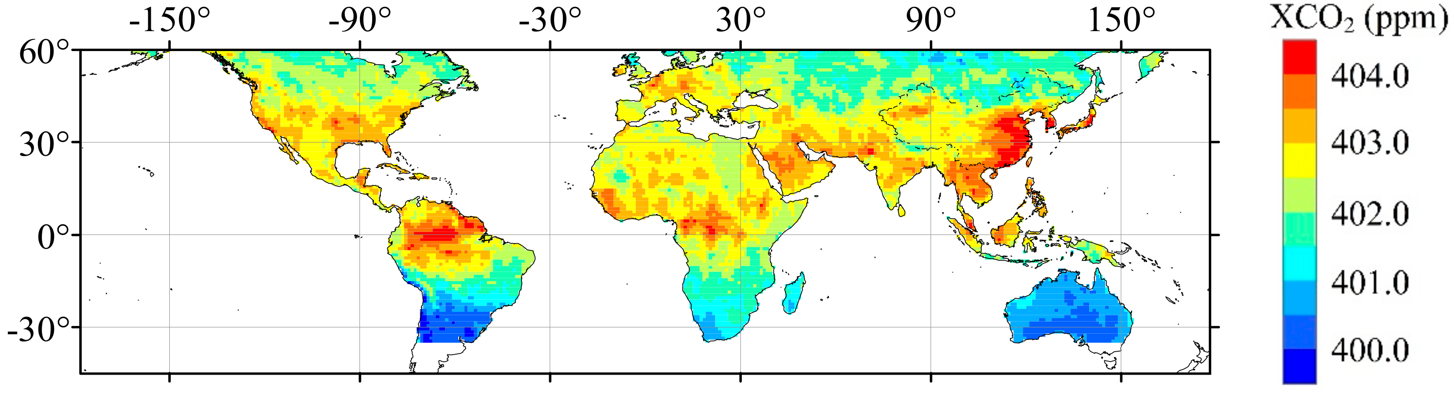
4.2.3. Spatial Distribution of GM-XCO2
4.3. GM-XCO2 Validation
4.3.1. Evaluation Using Cross-Validation
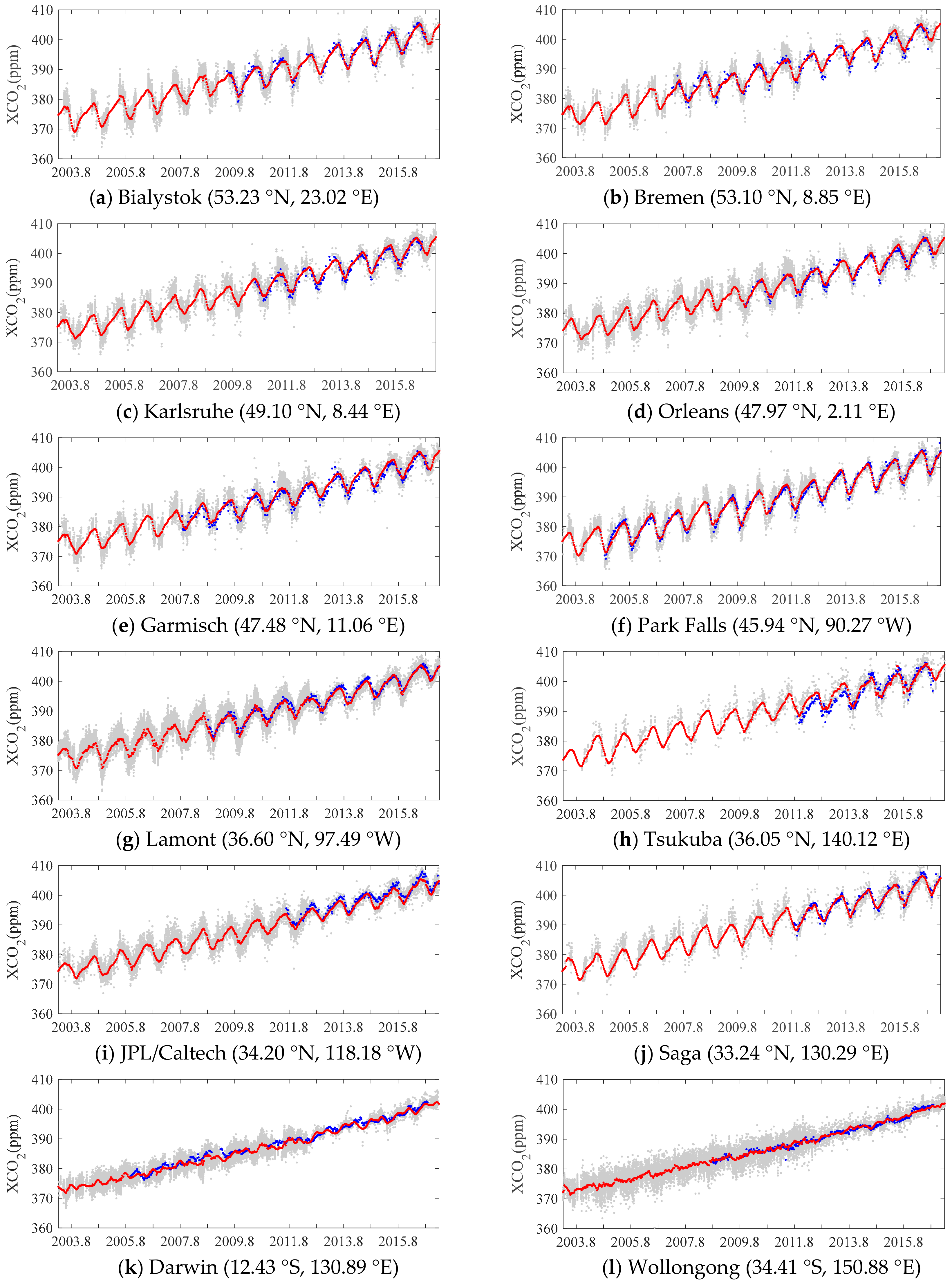
4.3.2. Validation of GM-XCO2 with TCCON Measurements
4.4. Comparison between GM-XCO2 and CarbonTracker Simulated XCO2
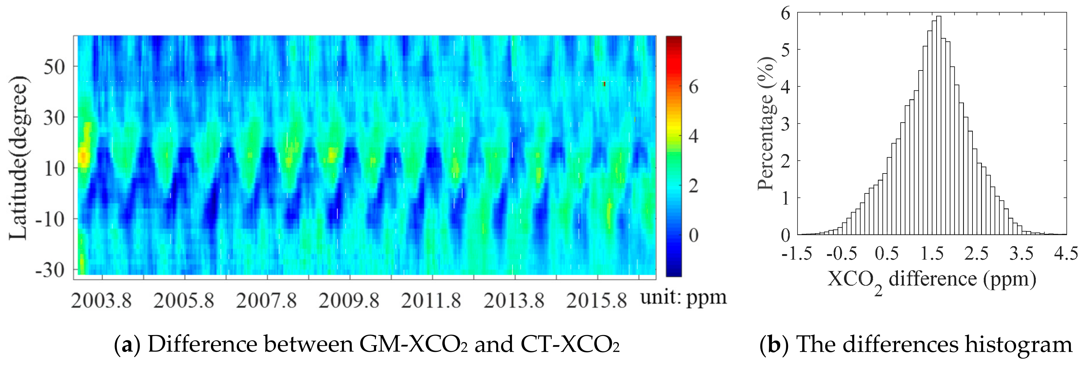
4.4.1. Comparison with Latitudinal and Temporal Variability of CT-XCO2
4.4.2. Temporal Variability of GM-XCO2 and CT-XCO2 in Mid-Latitudes
5. Discussion
6. Conclusions
Author Contributions
Funding
Acknowledgments
Conflicts of Interest
Appendix A


Acronyms
| Acronyms | Full Names |
| XCO2 | Column-averaged dry air mole fraction of atmospheric CO2 |
| Original XCO2 retrievals from satellites | |
| Adjusted | |
| Converted | |
| Integrated combination of | |
| GM-XCO2 | Global mapped XCO2 |
| ENVISAT | Environmental Satellite |
| SCIAMACHY | SCanning Imaging Absorption spectroMeter for Atmospheric CHartographY |
| GOSAT | Greenhouse Gases Observing Satellite |
| OCO-2 | Orbiting Carbon Observatory-2 |
| BESD | Bremen Optimal Estimation–DOAS |
| ACOS | Atmospheric CO2 Observations from Space |
| TCCON | The total carbon column observing network |
| CT | CarbonTracker |
| r2 | the coefficient of determination |
| RMSE | the root mean square error |
| ESRL | Earth System Research Laboratory |
References
- Le Quéré, C.; Andrew, R.M.; Friedlingstein, P.; Sitch, S.; Hauck, J.; Pongratz, J.; Pickers, P.A.; Korsbakken, J.I.; Peters, G.P.; Canadell, J.G.; et al. Global Carbon Budget 2018. Earth Syst. Sci. Data 2018, 10, 2141–2194. [Google Scholar] [CrossRef] [Green Version]
- Stocker, T.; Qin, D.; Plattner, G.; Tignor, M.; Allen, S.; Boschung, J.; Nauels, A.; Xia, Y.; Bex, B.; Midgley, B. IPCC, 2013: Climate Change 2013: The Physical Science Basis. In Contribution of Working Group I to the Fifth Assessment Report of the Intergovernmental Panel on Climate Change; Cambridge University Press: Cambridge, UK, 2013. [Google Scholar]
- Fortunat, J.; Renato, S. Rates of change in natural and anthropogenic radiative forcing over the past 20,000 years. Proc. Natl. Acad. Sci. USA 2008, 105, 1425–1430. [Google Scholar]
- Dlugokencky, E.; Tans, P. Trends in Atmospheric Carbon Dioxide, National Oceanic & Atmospheric Administration, Earth System Research Laboratory (NOAA/ESRL). Available online: http://www.esrl.noaa.gov/gmd/ccgg/trends/global.html (accessed on 19 October 2019).
- Le Quéré, C.; Moriarty, R.; Andrew, R.M.; Canadell, J.G.; Sitch, S.; Korsbakken, J.I.; Friedlingstein, P.; Peters, G.P.; Andres, R.J.; Boden, T.A.; et al. Global Carbon Budget 2015. Earth Syst. Sci. Data 2015, 7, 349–396. [Google Scholar] [CrossRef] [Green Version]
- Randerson, J.T.; Thompson, M.V.; Conway, T.J.; Fung, I.Y.; Field, C.B. The contribution of terrestrial sources and sinks to trends in the seasonal cycle of atmospheric carbon dioxide. Glob. Biogeochem. Cycles 1997, 11, 535–560. [Google Scholar] [CrossRef] [Green Version]
- He, Z.; Zeng, Z.-C.; Lei, L.; Bie, N.; Yang, S. A Data-Driven Assessment of Biosphere-Atmosphere Interaction Impact on Seasonal Cycle Patterns of XCO2 Using GOSAT and MODIS Observations. Remote Sens. 2017, 9, 251. [Google Scholar] [CrossRef] [Green Version]
- Graven, H.D.; Keeling, R.F.; Piper, S.C.; Patra, P.K.; Stephens, B.B.; Wofsy, S.C.; Welp, L.R.; Sweeney, C.; Tans, P.P.; Kelley, J.J. Enhanced Seasonal Exchange of CO2 by Northern Ecosystems Since 1960. Science 2013, 341, 1085–1089. [Google Scholar] [CrossRef] [Green Version]
- Zeng, N.; Zhao, F.; Collatz, G.J.; Kalnay, E.; Salawitch, R.J.; West, T.O.; Guanter, L. Agricultural Green Revolution as a driver of increasing atmospheric CO2 seasonal amplitude. Nature 2014, 515, 394–397. [Google Scholar] [CrossRef]
- Detmers, R.G.; Hasekamp, O.; Aben, I.; Houweling, S.; van Leeuwen, T.T.; Butz, A.; Landgraf, J.; Köhler, P.; Guanter, L.; Poulter, B. Anomalous carbon uptake in Australia as seen by GOSAT. Geophys. Res. Lett. 2015, 42, 8177–8184. [Google Scholar] [CrossRef] [Green Version]
- He, Z.; Lei, L.; Welp, L.; Zeng, Z.-C.; Bie, N.; Yang, S.; Liu, L. Detection of Spatiotemporal Extreme Changes in Atmospheric CO2 Concentration Based on Satellite Observations. Remote Sens. 2018, 10, 839. [Google Scholar] [CrossRef] [Green Version]
- Chevallier, F.; Palmer, P.I.; Feng, L.; Boesch, H.; O’Dell, C.W.; Bousquet, P. Toward robust and consistent regional CO2 flux estimates from in situ and spaceborne measurements of atmospheric CO2. Geophys. Res. Lett. 2014, 41, 1065–1070. [Google Scholar] [CrossRef] [Green Version]
- Deng, F.; Jones, D.B.A.; Henze, D.K.; Bousserez, N.; Bowman, K.W.; Fisher, J.B.; Nassar, R.; O’Dell, C.; Wunch, D.; Wennberg, P.O.; et al. Inferring regional sources and sinks of atmospheric CO2 from GOSAT XCO2 data. Atmos. Chem. Phys. 2014, 14, 3703–3727. [Google Scholar] [CrossRef] [Green Version]
- Eldering, A.; Wennberg, P.O.; Crisp, D.; Schimel, D.S.; Gunson, M.R.; Chatterjee, A.; Liu, J.; Schwandner, F.M.; Sun, Y.; O’Dell, C.W. The Orbiting Carbon Observatory-2 early science investigations of regional carbon dioxide fluxes. Science 2017, 358, eaam5745. [Google Scholar] [CrossRef] [PubMed] [Green Version]
- Ciais, P.; Dolman, A.J.; Bombelli, A.; Duren, R.; Peregon, A.; Rayner, P.J.; Miller, C.; Gobron, N.; Kinderman, G.; Marland, G.; et al. Current systematic carbon-cycle observations and the need for implementing a policy-relevant carbon observing system. Biogeosciences 2014, 11, 3547–3602. [Google Scholar] [CrossRef] [Green Version]
- Heimann, M. Searching out the sinks. Nat. Geosci. 2009, 2, 3–4. [Google Scholar] [CrossRef]
- Watanabe, H.; Hayashi, K.; Saeki, T.; Maksyutov, S.; Nasuno, I.; Shimono, Y.; Hirose, Y.; Takaichi, K.; Kanekon, S.; Ajiro, M.; et al. Global mapping of greenhouse gases retrieved from GOSAT Level 2 products by using a kriging method. Int. J. Remote Sens. 2015, 36, 1509–1528. [Google Scholar] [CrossRef] [Green Version]
- Kathryn, M.K.; Wofsy, S.C.; Thomas, N.; Janusz, E.; Ehleringer, J.R.; Stephens, B.B. Assessment of ground-based atmospheric observations for verification of greenhouse gas emissions from an urban region. Proc. Natl. Acad. Sci. USA 2012, 109, 8423–8428. [Google Scholar]
- Zeng, Z.-C.; Lei, L.; Strong, K.; Jones, D.B.A.; Guo, L.; Liu, M.; Deng, F.; Deutscher, N.M.; Dubey, M.K.; Griffith, D.W.T.; et al. Global land mapping of satellite-observed CO2 total columns using spatio-temporal geostatistics. Int. J. Digit. Earth 2016. [Google Scholar] [CrossRef] [Green Version]
- Kataoka, F.; Crisp, D.; Taylor, T.E.; O’Dell, C.W.; Lee, R.A.M. The Cross-Calibration of Spectral Radiances and Cross-Validation of CO2 Estimates from GOSAT and OCO-2. Remote Sens. 2017, 9, 1158. [Google Scholar] [CrossRef] [Green Version]
- Heymann, J.; Reuter, M.; Hilker, M.; Buchwitz, M.; Schneising, O.; Bovensmann, H.; Burrows, J.P.; Kuze, A.; Suto, H.; Deutscher, N.M.; et al. Consistent satellite XCO2 retrievals from SCIAMACHY and GOSAT using the BESD algorithm. Atmos. Meas. Tech. 2015, 8, 2961–2980. [Google Scholar] [CrossRef] [Green Version]
- Hakkarainen, J.; Ialongo, I.; Tamminen, J. Direct space-based observations of anthropogenic CO2 emission areas from OCO-2. Geophys. Res. Lett. 2016, 43, 11400–411406. [Google Scholar] [CrossRef]
- Bovensmann, H.; Buchwitz, M.; Burrows, J.P.; Reuter, M. A remote sensing technique for global monitoring of power plant CO2 emissions from space and related applications. Atmos. Meas. Tech. 2010, 3, 55–110. [Google Scholar] [CrossRef]
- Schwandner, F.M.; Gunson, M.R.; Miller, C.E.; Carn, S.A.; Eldering, A.; Krings, T.; Verhulst, K.R.; Schimel, D.S.; Nguyen, H.M.; Crisp, D. Spaceborne detection of localized carbon dioxide sources. Science 2017, 358, eaam5782. [Google Scholar] [CrossRef] [PubMed] [Green Version]
- Nassar, R.; Hill, T.G.; Mclinden, C.A.; Wunch, D.; Jones, D.B.A.; Crisp, D.; Nassar, R.; Hill, T.G.; Mclinden, C.A.; Wunch, D. Quantifying CO2 emissions from individual power plants from space. Geophys. Res. Lett. 2017, 44, 10045–10053. [Google Scholar] [CrossRef] [Green Version]
- Liu, J.; Bowman, K.W.; Schimel, D.S.; Parazoo, N.C.; Jiang, Z.; Lee, M.; Bloom, A.A.; Wunch, D.; Frankenberg, C.; Sun, Y.; et al. Contrasting carbon cycle responses of the tropical continents to the 2015–2016 El Nino. Science 2017, 358. [Google Scholar] [CrossRef] [Green Version]
- Feng, L.; Palmer, P.I.; Parker, R.J.; Deutscher, N.M.; Feist, D.G.; Kivi, R.; Morino, I.; Sussmann, R. Estimates of European uptake of CO2 inferred from GOSAT XCO2 retrievals: Sensitivity to measurement bias inside and outside Europe. Atmos. Chem. Phys. 2016, 16, 1289–1302. [Google Scholar] [CrossRef] [Green Version]
- Bovensmann, H.; Burrows, J.P.; Buchwitz, M.; Frerick, J.; Noël, S.; Rozanov, V.V.; Chance, K.V.; Goede, A.P.H. SCIAMACHY: Mission Objectives and Measurement Modes. J. Atmos. Sci. 1999, 56, 125–150. [Google Scholar] [CrossRef] [Green Version]
- Yokota, T.; Yoshida, Y.; Eguchi, N.; Ota, Y.; Tanaka, T.; Watanabe, H.; Maksyutov, S. Global concentrations of CO2 and CH4 retrieved from GOSAT: First preliminary results. Sci. Online Lett. Atmos. 2009, 5, 160–163. [Google Scholar] [CrossRef] [Green Version]
- Boesch, H.; Baker, D.; Connor, B.; Crisp, D.; Miller, C. Global Characterization of CO2 Column Retrievals from Shortwave-Infrared Satellite Observations of the Orbiting Carbon Observatory-2 Mission. Remote Sens. 2011, 3, 270–304. [Google Scholar] [CrossRef] [Green Version]
- Zeng, Z.; Lei, L.; Hou, S.; Ru, F.; Guan, X.; Zhang, B. A Regional Gap-Filling Method Based on Spatiotemporal Variogram Model of Columns. IEEE Trans. Geosci. Remote Sens. 2014, 52, 3594–3603. [Google Scholar] [CrossRef]
- Hammerling, D.M.; Michalak, A.M.; O’Dell, C.; Kawa, S.R. Global CO2 distributions over land from the Greenhouse Gases Observing Satellite (GOSAT). Geophys. Res. Lett. 2012, 39, 1–6. [Google Scholar] [CrossRef] [Green Version]
- Hai, N.; Katzfuss, M.; Cressie, N.; Braverman, A. Spatio-Temporal Data Fusion for Very Large Remote Sensing Datasets. Technometrics 2014, 56, 174–185. [Google Scholar]
- Liu, Y.; Wang, X.; Guo, M.; Tani, H. Mapping the FTS SWIR L2 product of XCO2 and XCH4 data from the GOSAT by the Kriging method—A case study in East Asia. Int. J. Remote Sens. 2012, 33, 3004–3025. [Google Scholar] [CrossRef] [Green Version]
- Jing, Y.; Shi, J.; Wang, T.; Sussmann, R. Mapping global atmospheric CO2 concentration at high spatiotemporal resolution. Atmosphere 2014, 5, 870–888. [Google Scholar] [CrossRef] [Green Version]
- Tadi, J.M.; Qiu, X.; Miller, S.; Michalak, A.M. Spatio-temporal approach to moving window block kriging of satellite data. Geosci. Model Dev. 2017, 10, 1–17. [Google Scholar] [CrossRef] [Green Version]
- Reuter, M.; Bovensmann, H.; Buchwitz, M.; Burrows, J.P.; Connor, B.J.; Deutscher, N.M.; Griffith, D.W.T.; Heymann, J.; Keppel-Aleks, G.; Messerschmidt, J.; et al. Retrieval of atmospheric CO2 with enhanced accuracy and precision from SCIAMACHY: Validation with FTS measurements and comparison with model results. J. Geophys. Res. 2011, 116. [Google Scholar] [CrossRef] [Green Version]
- O’Dell, C.W.; Connor, B.; Bösch, H.; O’Brien, D.; Frankenberg, C.; Castano, R.; Christi, M.; Eldering, D.; Fisher, B.; Gunson, M.; et al. The ACOS CO2 retrieval algorithm—Part 1: Description and validation against synthetic observations. Atmos. Meas. Tech. 2012, 5, 99–121. [Google Scholar] [CrossRef] [Green Version]
- Wunch, D.; Wennberg, P.O.; Osterman, G.; Fisher, B.; Naylor, B.; Roehl, C.M.; Dell, C.; Mandrake, L. Comparisons of the Orbiting Carbon Observatory-2 (OCO-2) XCO2 measurements with TCCON. Atmos. Meas. Tech. 2017, 10, 2209–2238. [Google Scholar] [CrossRef] [Green Version]
- Wunch, D.; Wennberg, P.O.; Toon, G.C.; Connor, B.J.; Fisher, B.; Osterman, G.B.; Frankenberg, C.; Mandrake, L.; O’Dell, C.; Ahonen, P.; et al. A method for evaluating bias in global measurements of CO2 total columns from space. Atmos. Chem. Phys. 2011, 11, 12317–12337. [Google Scholar] [CrossRef] [Green Version]
- Liang, A.; Gong, W.; Han, G.; Xiang, C. Comparison of Satellite-Observed XCO2 from GOSAT, OCO-2, and Ground-Based TCCON. Remote Sens. 2017, 9, 1033. [Google Scholar] [CrossRef] [Green Version]
- Peters, W.; Jacobson, A.R.; Sweeney, C.; Andrews, A.E.; Conway, T.J.; Masarie, K.; Miller, J.B.; Bruhwiler, L.M.; Petron, G.; Hirsch, A.I.; et al. An atmospheric perspective on North American carbon dioxide exchange: CarbonTracker. Proc. Natl. Acad. Sci. USA 2007, 104, 18925–18930. [Google Scholar] [CrossRef] [Green Version]
- Connor, B.J.; Boesch, H.; Toon, G.; Sen, B.; Miller, C.; Crisp, D. Orbiting Carbon Observatory: Inverse method and prospective error analysis. J. Geophys. Res. Atmos. 2008, 113, 1–14. [Google Scholar] [CrossRef]
- Rodgers, C.D.; Connor, B.J. Intercomparison of remote sounding instruments. J. Geophys. Res. Atmos. 2003, 108. [Google Scholar] [CrossRef] [Green Version]
- Wang, T.; Shi, J.; Jing, Y.; Zhao, T.; Ji, D.; Xiong, C. Combining XCO2 measurements derived from SCIAMACHY and GOSAT for potentially generating global CO2 maps with high spatiotemporal resolution. PLoS ONE 2014, 11, e0148152. [Google Scholar] [CrossRef] [PubMed]
- Olsen, S.C.; Randerson, J.T. Differences between surface and column atmospheric CO2 and implications for carbon cycle research. J. Geophys. Res. Atmos. 2004, 109. [Google Scholar] [CrossRef] [Green Version]
- Kevin Robert, G.; Law, R.M.; Scott, D.; Rayner, P.J.; David, B.; Philippe, B.; Lori, B.; Yu-Han, C.; Philippe, C.; Songmiao, F. Towards robust regional estimates of CO2 sources and sinks using atmospheric transport models. Nature 2002, 415, 626–630. [Google Scholar]
- Lindqvist, H.; O’Dell, C.W.; Basu, S.; Boesch, H.; Chevallier, F.; Deutscher, N.; Feng, L.; Fisher, B.; Hase, F.; Inoue, M.; et al. Does GOSAT capture the true seasonal cycle of carbon dioxide? Atmos. Chem. Phys. 2015, 15, 13023–13040. [Google Scholar] [CrossRef] [Green Version]
- Cogan, A.J.; Boesch, H.; Parker, R.J.; Feng, L.; Palmer, P.I.; Blavier, J.F.L.; Deutscher, N.M.; Macatangay, R.; Notholt, J.; Roehl, C.; et al. Atmospheric carbon dioxide retrieved from the Greenhouse gases Observing SATellite (GOSAT): Comparison with ground-based TCCON observations and GEOS-Chem model calculations. J. Geophys. Res. Atmos. 2012, 117, 1–17. [Google Scholar] [CrossRef] [Green Version]
- Kyriakidis, P.C.; Journel, A.G. Geostatistical Space–Time Models: A Review. Math. Geol. 1999, 31, 651–684. [Google Scholar] [CrossRef]
- De Iaco, S. Space–time correlation analysis: A comparative study. J. Appl. Stat. 2010, 37, 1027–1041. [Google Scholar] [CrossRef]
- Iaco, S.D.; Myers, D.E.; Posa, D. Space–time analysis using a general product–sum model. Stat. Probab. Lett. 2001, 52, 21–28. [Google Scholar] [CrossRef]
- Cressie, N.; Wikle, C.K. Statistics for Spatio-Temporal Data; Wily: New York, NY, USA, 2011. [Google Scholar]
- Liu, M.; Lei, L.; Liu, D.; Zeng, Z.-C. Geostatistical Analysis of CH4 Columns over Monsoon Asia Using Five Years of GOSAT Observations. Remote Sens. 2016, 8, 361. [Google Scholar] [CrossRef] [Green Version]
- Schneising, O.; Heymann, J.; Buchwitz, M.; Reuter, M.; Bovensmann, H.; Burrows, J.P. Anthropogenic carbon dioxide source areas observed from space: Assessment of regional enhancements and trends. Atmos. Chem. Phys. 2013, 13, 2445–2454. [Google Scholar] [CrossRef] [Green Version]
- Miller, C.E.; Crisp, D.; Decola, P.L.; Olsen, S.C.; Randerson, J.T.; Michalak, A.M.; Alkhaled, A.; Rayner, P.; Jacob, D.J.; Suntharalingam, P. Precision requirements for space-based XCO2 data. Ir. J. Psychol. Med. 2007, 29, 143–145. [Google Scholar]
- Wu, L.; aan de Brugh, J.; Meijer, Y.; Sierk, B.; Hasekamp, O.; Butz, A.; Landgraf, J. XCO2 observations using satellite measurements with moderate spectral resolution: Investigation using GOSAT and OCO-2 measurements. Atmos. Meas. Tech. Discuss. 2019, 2019, 1–23. [Google Scholar] [CrossRef]
- Belikov, D.A.; Bril, A.; Maksyutov, S.; Oshchepkov, S.; Saeki, T.; Takagi, H.; Yoshida, Y.; Ganshin, A.; Zhuravlev, R.; Aoki, S.; et al. Column-averaged CO2 concentrations in the subarctic from GOSAT retrievals and NIES transport model simulations. Polar Sci. 2014, 8, 129–145. [Google Scholar] [CrossRef] [Green Version]
- Kong, Y.; Chen, B.; Measho, S. Spatio-Temporal Consistency Evaluation of XCO2 Retrievals from GOSAT and OCO-2 Based on TCCON and Model Data for Joint Utilization in Carbon Cycle Research. Atmosphere 2019, 10, 354. [Google Scholar] [CrossRef] [Green Version]
- Yoshida, Y.; Kikuchi, N.; Morino, I.; Uchino, O.; Oshchepkov, S.; Bril, A.; Saeki, T.; Schutgens, N.; Toon, G.C.; Wunch, D.; et al. Improvement of the retrieval algorithm for GOSAT SWIR XCO2 and XCH4 and their validation using TCCON data. Atmos. Meas. Tech. 2013, 6, 1533–1547. [Google Scholar] [CrossRef]


| Attributes\Satellites | ENVISAT/SCIAMACHY | GOSAT | OCO-2 |
|---|---|---|---|
| Period of selected data | January 2003–March 2012 | June 2009–May 2016 | September 2014–December 2016 |
| Repeat cycle (days) | 35 | 3 | 16 |
| Field of view (km) | 30 × 60 | Diameter of 10.5 | 2.25×1.25 |
| Overpass local time | 10:00 | 13:00 | 13:36 |
| version | BESD v02.01.01 | ACOS v7.3 | OCO2 r9 |
| Profile layers number | 10 | 20 | 20 |
| Criteria of data screening | XCO2_quality_flag=0; | XCO2_quality_flag=0; gain=H; land_fraction>90; warn_level<10 | XCO2_quality_flag=0; gain=H; land_fraction>90 |
| Name referred hereafter | SCI-XCO2 | GOS-XCO2 | OCO-XCO2 |
| Reference | [37] | [38] | [39] |
| Sites | Location (Latitude, Longitude) | Coincident Data Pairs | Averaged Bias (ppm) | Averaged Absolute Bias (ppm) | Standard Deviation (ppm) |
|---|---|---|---|---|---|
| Bialystok | (53.23°N, 23.02°E) | 249 | −0.19 | 0.73 | 0.92 |
| Bremen | (53.10°N, 8.85°E) | 260 | 0.21 | 0.97 | 1.25 |
| Karlsruhe | (49.10°N, 8.44°E) | 226 | 0.51 | 0.90 | 0.98 |
| Orleans | (47.97°N, 2.11°E) | 232 | 0.34 | 0.71 | 0.85 |
| Garmisch | (47.48°N, 11.06°E) | 361 | 0.62 | 1.05 | 1.16 |
| Park Falls | (45.94°N, 90.27°W) | 499 | 0.00 | 0.74 | 0.96 |
| Lamont | (36.60°N, 97.49°W) | 381 | −0.45 | 0.77 | 0.92 |
| Tsukuba | (36.05°N, 140.12°E) | 210 | 0.73 | 1.70 | 1.89 |
| JPL/Caltech | (34.20°N, 118.18°W) | 243 | −1.06 | 1.19 | 0.97 |
| Saga | (33.24°N, 130.29°E) | 204 | −0.33 | 0.76 | 0.91 |
| Darwin | (12.43°S, 130.89°E) | 434 | −0.47 | 0.89 | 1.00 |
| Wollongong | (34.41°S, 150.88°E) | 341 | 0.09 | 0.58 | 0.75 |
| Overall | - | 303 | 0.01 | 0.92 | 1.05 |
© 2020 by the authors. Licensee MDPI, Basel, Switzerland. This article is an open access article distributed under the terms and conditions of the Creative Commons Attribution (CC BY) license (http://creativecommons.org/licenses/by/4.0/).
Share and Cite
He, Z.; Lei, L.; Zhang, Y.; Sheng, M.; Wu, C.; Li, L.; Zeng, Z.-C.; Welp, L.R. Spatio-Temporal Mapping of Multi-Satellite Observed Column Atmospheric CO2 Using Precision-Weighted Kriging Method. Remote Sens. 2020, 12, 576. https://0-doi-org.brum.beds.ac.uk/10.3390/rs12030576
He Z, Lei L, Zhang Y, Sheng M, Wu C, Li L, Zeng Z-C, Welp LR. Spatio-Temporal Mapping of Multi-Satellite Observed Column Atmospheric CO2 Using Precision-Weighted Kriging Method. Remote Sensing. 2020; 12(3):576. https://0-doi-org.brum.beds.ac.uk/10.3390/rs12030576
Chicago/Turabian StyleHe, Zhonghua, Liping Lei, Yuhui Zhang, Mengya Sheng, Changjiang Wu, Liang Li, Zhao-Cheng Zeng, and Lisa R. Welp. 2020. "Spatio-Temporal Mapping of Multi-Satellite Observed Column Atmospheric CO2 Using Precision-Weighted Kriging Method" Remote Sensing 12, no. 3: 576. https://0-doi-org.brum.beds.ac.uk/10.3390/rs12030576