Enhanced Delaunay Triangulation Sea Ice Tracking Algorithm with Combining Feature Tracking and Pattern Matching

Abstract

Sea ice drift detection has the key role of global climate analysis and waterway planning. The ability to detect sea ice drift in real-time also contributes to the safe navigation of ships and the prevention of offshore oil platform accidents. In this paper, an Enhanced Delaunay Triangulation (EDT) algorithm for sea ice tracking was proposed for dual-polarization sequential Synthetic Aperture Radar (SAR) images, which was implemented by combining feature tracking with pattern matching based on integrating HH and HV polarization feature information. A sea ice retrieval algorithm for feature detection, matching, fusion, and outlier detection was specifically developed to increase the system’s accuracy and robustness. In comparison with several state-of-the-art sea ice drift retrieval algorithms, including Speeded Up Robust Features (SURF) and the Oriented FAST and Rotated BRIEF (ORB) method, the results of the experiment provided compelling evidence that our algorithm had a higher accuracy than the SURF and ORB method. Furthermore, the results of our method were compared with the drift vector and direction of buoys data. The drift direction is consistent with buoys, and the velocity deviation was about 10 m. It was proved that this method can be applied effectively to the retrieval of sea ice drift.

1. Introduction

Sea ice drift has an essential influence on the distribution of sea ice on different temporal and spatial scales, and presents a potential risk for navigation and other industrial activities [1]. Nowadays, monitoring sea ice drift is not only crucial for safe navigation, but also greatly crucial to climate analysis for all of the world. However, due to the lack of ground stations in sea ice-covered areas, there is still a shortage of dependable sea ice drift products for the application.

With the development of science and technology, a large number of tools are used to observe sea ice conditions. Sea ice drift was first measured with ship observations by Nansens expedition in 1893–1896 [2]. Since 1979, the International Arctic Buoy Programme (IABP) has installed about 20 buoys per year to build a network of buoy data to monitor sea level pressure, surface air temperature, and ice motion throughout the Arctic Ocean. These buoys data can provide continuous local measurements, but the spatial distribution is too sparse to provide a large area of the velocity field. In order to effectively observe and predict sea ice motion, it is necessary to obtain the movement of sea ice on large scales. Since the 1990s, with the development of satellite remote sensing technology, sea ice drift has been estimated from satellite data with daily and global coverage of the polar oceans [3,4,5,6]. Thus, the coverage scale problem was effectively solved. Currently, the most commonly satellite sensors include Advanced Very High-Resolution Radiometer (AVHRR) [7,8,9], SeaWinds/QuikSCAT enhanced resolution data [10], Special Sensor Microwave/Imager (SSM/I) [11,12,13], and Synthetic Aperture Radar (SAR) [14,15,16,17,18]. The microwave radiometers and scatter meters customarily monitor large-scale sea ice drift, but due to their limited resolution, the local movement of sea ice cannot be obtained. Fowler et al. [19] used a combination of the Scanning Multichannel Microwave Radiometer (SMMR), SSM/I, AVHRR, and the optical data to first compute the daily movement of Arctic sea ice from sequential satellite images using the maximum-cross correlation (MCC) method, and obtained sea ice motion vectors by merging ice motions from satellite-based infrared and multichannel microwave (MW) images, buoy measurements, and reanalysis data [20,21]. These approaches are efforts to overcome the resolution problem of passive microwave measurement. Nowadays, the Synthetic Aperture Radar (SAR) has the advantages of high temporal resolution and large spatial coverage, which are desirable for monitoring the rapid motion of sea ice. Sentinel-1 SAR is one of desirable satellite, which is a polar-orbiting, all-weather, day-and-night radar imaging mission for land and ocean services. Currently, the Sentinel-1A and B together provide frequent and reliable data, which will provide significant observations for the Arctic. As the amount of SAR imagery is growing, improving the efficiency of the sea ice drift retrieval algorithms is required.

In the past decades, several methods have estimated sea ice drift with satellite sensors data, including pattern matching, feature tracking, and optical flow [22], as well as the combination of different methods. The pattern matching methods include the maximum cross-correlation (MCC) [2,23] and phase-correlation (PC) [24] method. The MCC method has proven to be robust and simple and has been well-validated, but the computational inefficiency limits its widespread application and it cannot capture the rotational component of sea ice motion. The PC method uses the Fast Fourier Transform (FFT), so its computational efficiency is several times faster than the MCC algorithm [25] and it has the ability to monitor the rotation sea ice motion, but a weakness is that the peak value in the phase correlation matrix does not provide an evident measure of similarity between two sub-images [26]. The feature tracking method contains Scale-Invariant Feature Transform (SIFT) [27,28], Speeded Up Robust Features (SURF) [29], Oriented FAST and Rotated BRIEF (ORB) [30], and other enhanced versions [31,32,33]. This kind of algorithm can detect features from sequential images and can optimize feature correspondence. Compared with the MCC method, it is more computationally efficient to handle shear zones, rotation, and divergence/convergence zones, but the resulting features may be unevenly distributed in space, and large gaps may occur between features vectors [34].

In order to resolve the above problems, an Enhanced Delaunay Triangulation (EDT) sea ice tracking algorithm that combines with feature tracking and pattern matching was proposed to monitor sea ice drift with high-resolution dual-polarization Sequential Sentinel-1 SAR images. The remainder of this paper is divided into four sections. Section 2 introduces the study area and SAR data. In Section 3, some details of our sea ice drift algorithm are described. Section 4 presents the results of the experimental and the EDT algorithm performance in comparison with other state-of-the-art methods. Finally, Section 5 gives the conclusions and future avenues for research.

2. Study Area and Data

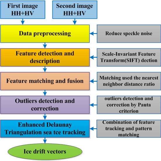
The Sentinel-1 mission includes two satellites, Sentinel-1A (launched in April 2014) and Sentinel-1B (launched in April 2016), each carrying a single C-band SAR with a center frequency of 5.405 GHz. The most commonly used mode of the Sentinel-1 on sea, glacier, and polar areas is the Extra Wide mode Ground Range Detected Medium Resolution (EW GRDM), which can cover an area of 400 km × 400 km per image with a resolution of 40 m × 40 m. Also, its excellent coverage performance and revisit performance can cover the entire European and Canadian regions and the surrounding maritime areas in a single day, which provides strong support for monitoring sea ice drift. The Sentinel-1 C-band SAR sensor supports single polarization (HH/VV) and dual polarization (HH + HV and VV + VH). We used two pairs of dual-polarization (HH + HV) images acquired over the Beaufort Sea to illustrate the method performance, which are shown in Figure 1, and the data information are shown in

Table 1. List of Sentinel-1 SAR images used in this paper.

Datasets	Start Time	End Time	Geographic Extent	Dual Polarization
1	2017-10-10 17:11:42	2017-10-12 16:55:20	79°01′—81°45′N 119°42′—134°25′W	HH + HV
2	2017-10-16 16:23:34	2017-10-18 16:07:14	76°52′—78°15′N 140°49′—157°06′W	HH + HV

.

3. Methods

Our sea ice drift algorithm is based on multi-polarization Sequential SAR images and is designed to combine feature tracking and pattern matching. As described in the flowchart in Figure 2, the algorithm included five main stages: (A) Data preprocessing, (B) feature detection and description, (C) feature matching and fusion, (D) outlier detection and correction, and (E) enhanced Delaunay Triangulation sea ice tracking.

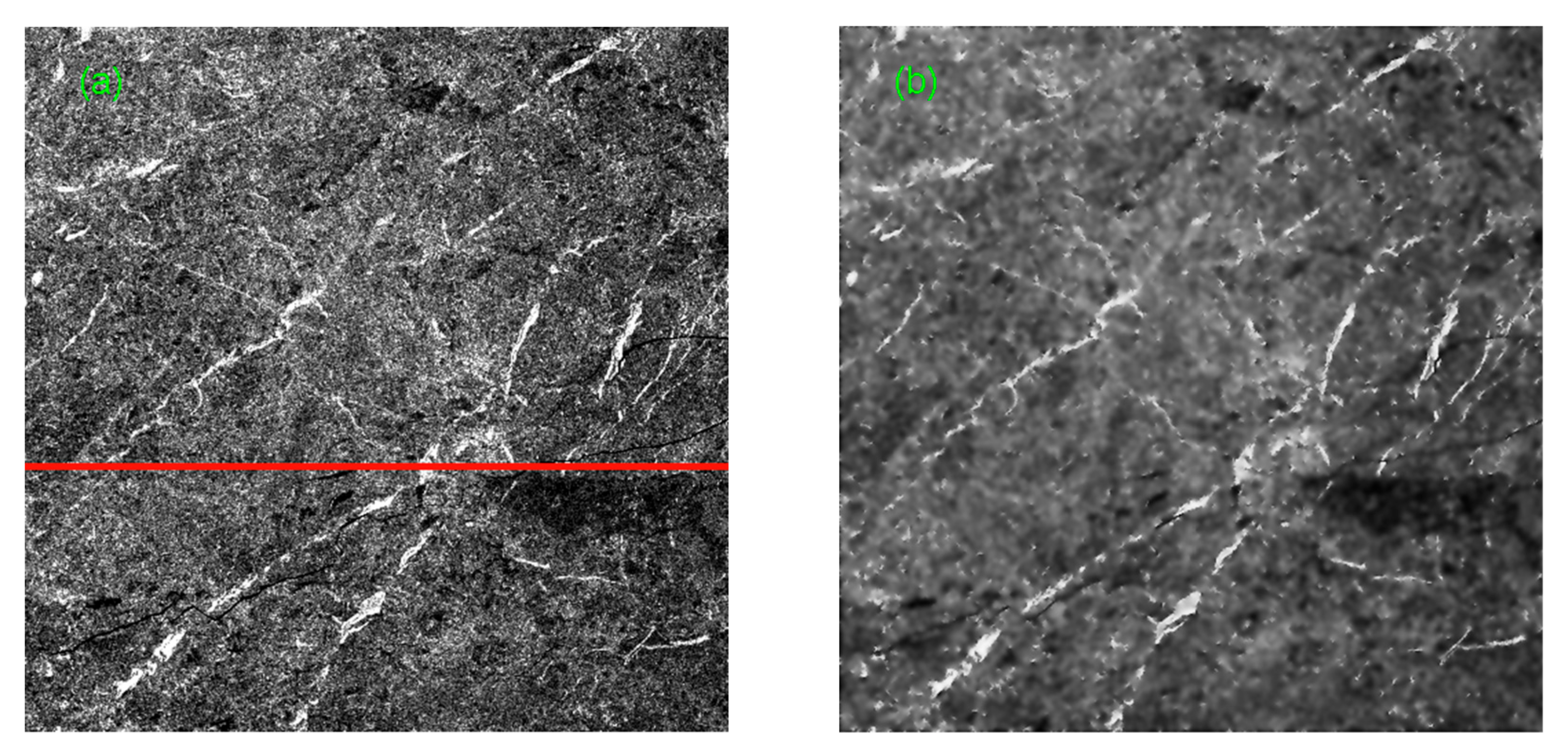
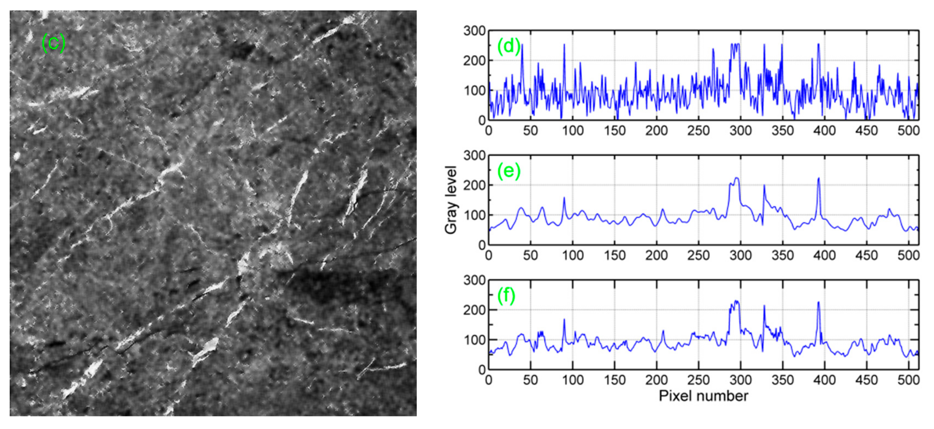
3.1. Data Preprocessing

The preprocessing of Sentinel-1 data was performed as follows. First, the normalized radar cross section was calculated as follows:

$${\sigma }^0=\frac{D{N}_i^2}{A_i^2}$$

(1)

where ${\sigma }^0$ denotes the normalized radar cross section, $D{N}_i$ represents the digital number provided in the source TIFF file, and $A_i^2$ expresses the value of normalization coefficient and $i$ is an index of a pixel [30].

In order to effectively extract feature information, the normalized radar cross section ${\sigma }^0$ has to be transformed into intensity values. This transformation was calculated as follows:

$$i=255\cdot \frac{{\sigma }^0-{\sigma }_{\min }^0}{{\sigma }_{\max }^0-{\sigma }_{\min }^0}\hspace{1em}0\le i\le 255$$

(2)

The next stage was denoising processing for the input SAR images to reduce the SAR speckle noise and preserve the edge details and object boundaries. In this paper, we used the image despeckling convolutional neural network (ID-CNN) method [35], which can automatically remove speckle from the input noisy images.

In order to select an effective denoising method, we compared the result of SAR block-matching 3-D (SAR-BM3D) [36] with the ID-CNN [35] method. The experimental results are shown in the Figure 3. Figure 3a shows the original SAR image, while Figure 3b,c show the results of the SAR block-matching 3-D (SAR-BM3D) method [36] and ID-CNN method [35], respectively. We selected a row of SAR image data with a red line to compare the spatial intensity changes as shown in Figure 3a. Figure 3d–f shows the spatial luminance profile changes for the unfiltered SAR image, filtered by the SAR-BM3D and ID-CNN method, respectively. The advantages of using the ID-CNN compared with the SAR-BM3D method are obvious, as the SAR-BM3D method produces over-smooth edges, and many details may be lost during the processing of despeckling. In contrast, the INCNN not only reserved the sharp edges and fine details, but also achieved visually pleasant results in the smooth region. Thus, this advantage is beneficial to subsequent feature extraction.

3.2. Feature Detection and Description

The second step is feature detection, which is used Scale-Invariant Feature Transform (SIFT) algorithm [27]. This algorithm attempts to obtain scale-invariant features using a staged filtering method. In our method, the scale space of a SAR image can be defined as $L\left(x,y,\sigma \right)$, which is calculated as:

$$L\left(x,y,\sigma \right)=G\left(x,y,\sigma \right)\ast I\left(x,y\right)$$

(3)

where the $G\left(x,y,\sigma \right)$ stands for variable-scale Gaussian function, calculated as $G\left(x,y,\sigma \right)=\frac{1}{2\pi {\sigma }^2}{\mathrm{e}}^{-\left(x^2+y^2\right)/2{\sigma }^2}$, $\sigma$ stands for the scale space factor, $I\left(x,y\right)$ represents the original SAR image, and $\ast$ is the convolution operation in $x$ and $y$.

In order to detect stable key point locations in the scale space, we obtained the scale-space extreme $D\left(x,y,\sigma \right)$ from the difference of Gaussians function convolved with the SAR image $I\left(x,y\right)$.

$$\begin{array}{ll}D\left(x,y,\sigma \right)& =\left(G\left(x,y,k\sigma \right)-G\left(x,y,\sigma \right)\right)\ast I\left(x,y\right)\\ & =L\left(x,y,k\sigma \right)-L\left(x,y,\sigma \right)\end{array}$$

(4)

where $k$ is a constant multiplicative factor.

For the sake of obtaining the local maxima and minima of $D\left(x,y,\sigma \right)$, each sample point was compared to the eight neighbors in the scale space. It was selected only if it was larger than all of these neighbors or smaller than all of them. Then, we assigned a consistent orientation to each key point.

3.3. Feature Matching and Fusion

Once the feature descriptors have been obtained from the extracted key points, the next step is feature matching. Feature matching aims to establish a set of correspondences between features from two or multiple SAR images. In this section, we used the Euclidean distance to measure the similarity between two features. For more efficient matching, we used the nearest neighbor distance ratio (NNDR) [27] to verify matching. The match is correct can be verified by the ratio of the distance from the closest neighbor to that of the second closest neighbor. In our experiment, we set the distance ratio to 0.8, which can filter out 90% of the false matches while eliminating less than 5% of the correct matches. In this paper, we extracted features from HH and HV polarization, respectively. We found that the key points from HH and HV polarization had different location information, so we fused the feature points. The experiment details are discussed in Section 4.1.

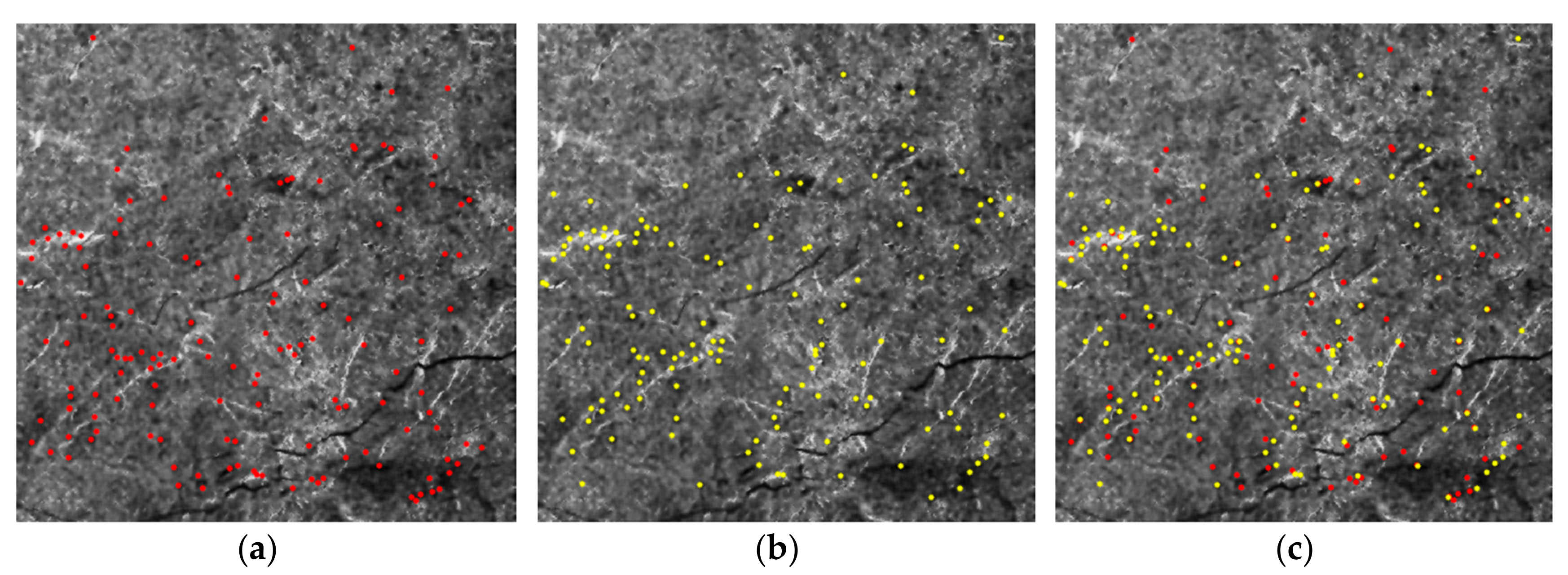
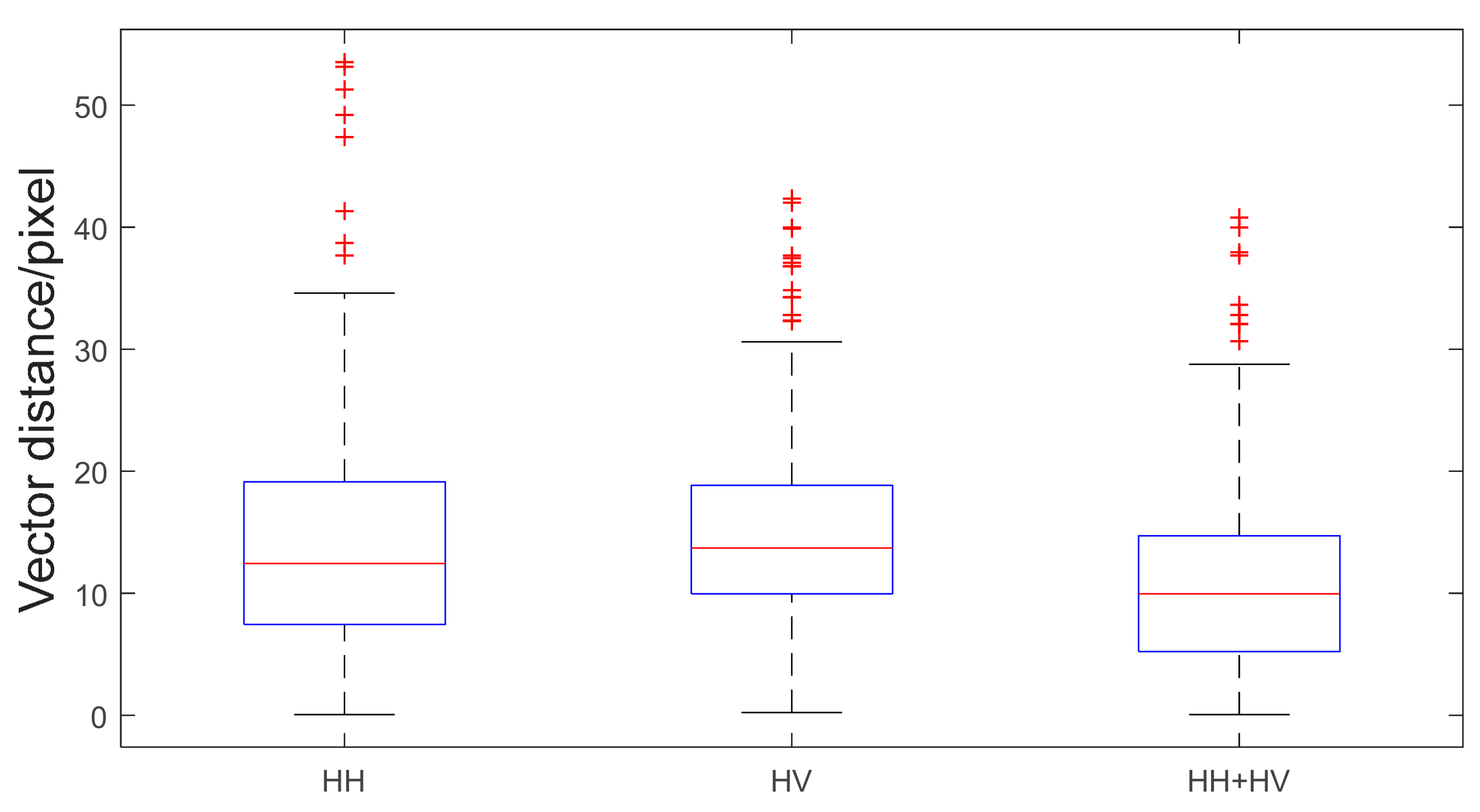
3.4. Outliers Detection and Correction

In this paper, we focused on improving the robustness of the method. In order to reduce the impact of potentially feature vectors on the following steps, we used the Pauta Criterion to eliminate the outliers. The Pauta Criterion was proposed for the outlier filtering of the sample data. The process of detecting outliers by the Pauta Criterion can be listed as follows:

$$\mathrm{p}\left(x\right)=\left\{\begin{array}{l}0.68\\ 0.95\\ 0.99\end{array}\right.\begin{array}{l}\mathrm{if} x\in (\mu -\sigma ,\mu +\sigma )\\ \mathrm{if} x\in (\mu -2\sigma ,\mu +2\sigma )\\ \mathrm{if} x\in (\mu -3\sigma ,\mu +3\sigma )\end{array}$$

(5)

where $\mu$ and $\sigma$ denote the mean and standard values of the sample data, respectively. The basic thought of the Pauta Criterion is to set a confidence interval to remove the outliers. When the measured data is within the (μ − 3σ, μ + 3σ) range, 0.1% of data are the outliers, which are not desirable, so these data should be removed from the measured data. In this paper, in order to effectively remove outliers, we set confidence intervals within (μ − σ, μ + σ), which can filter out more false matches while preserving more correct matches. The experiment details are discussed in Section 4.2.

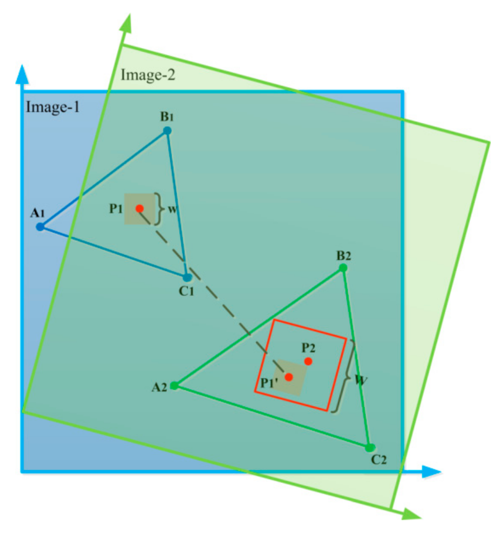
3.5. Enhanced Delaunay Triangulation Sea Ice Tracking Algorithm

The proposed sea ice drift retrieved method is based on the feature tracking and pattern matching. First, using the feature points obtained by the above method, we constructed a triangular network based on the locations of feature points by the Delaunay Triangulation algorithm [37,38,39] as shown in Figure 4. Second, we selected one group of the corresponding triangle A₁B₁C₁ and A₂B₂C₂ from the first image (Image-1) and the second image (Image-2) as shown in Figure 5. Then, we calculated the center of gravity P₁ and P₂ of each triangle as illustrated by Figure 5, and a group of new feature points was obtained. However, there were still some open problems that needed to be solved, including the fact that that feature points P₁ and P₂ may not be optimally matched. In order to solve this problem, we used a pattern matching algorithm to obtain optimal and feature points.

In our experiments, the pattern matching method was based on the maximum cross-correlation (MCC) method. Considering a small sub-image $I_1$ around the point of interest $p_1\left(x_1,y_1\right)$ from the Image-1 with size 50×50 (gray square) and a larger sub-image around the point $p_2\left(x_2,y_2\right)$ from the Image-2 with size 200×200 (red square), the normalized cross-correlation matrix NCC [40,41] was defined as:

$$NCC\left(x,y\right)=\frac{{\displaystyle \sum I_1\cdot I_2}}{\sqrt{\left({\displaystyle \sum I_1\cdot I_1}\right)\times \left({\displaystyle \sum I_2\cdot I_2}\right)}}$$

(6)

where $I_1\in R^{50\times 50},I_2\in R^{50\times 50}$. In the matrix NCC, we obtained the maximum normalized cross-correlation value, and its coordinate value represents the best match point $p_1^{\prime }\left(x_1^{\prime },y_1^{\prime }\right)$ in the second image.

$$\left(x_1^{\prime },y_1^{\prime }\right)=\stackrel{\arg \max }{\left(x,y\right)}\left(NCC\left(x,y\right)\right)$$

(7)

To explain the pattern matching process, an example is shown in Figure 5. A sub-image was selected from the first image (as shown in Figure 6a with a green empty square). Cross-correlations were computed between the sub-image, with a large search area in the second image (as shown in Figure 6b with a yellow empty square). Figure 6c shown the cross-correlation matrix. The sub-image (as shown in Figure 6b with a red empty square) is the area that produced the highest maximum cross-correlation coefficient with the sub-image (yellow empty square) in the first image. As shown in Figure 6b, the drift vector of the sea ice is the deviation between the green empty square and the red empty square.

4. Experimental Results and Discussion

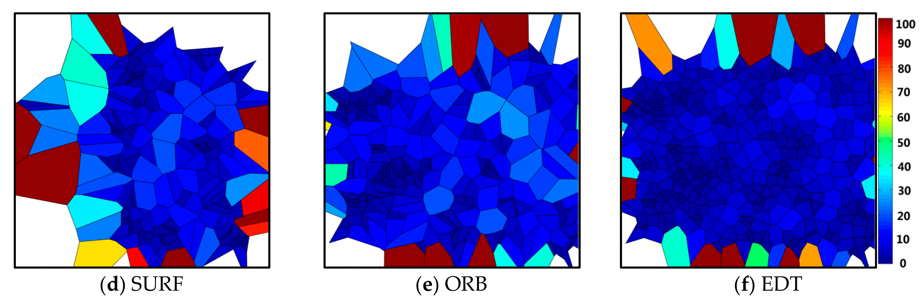
4.1. Compared the Performance of Feature Extraction

In our experiment, we extracted features from HH and HV polarization, respectively. These features points were matched by the NNDR [27] method, and the result can be seen in Figure 7a,b, in which we obtained 155 and 141 key points from the HH and HV polarization image, respectively. Comparing Figure 7a,b, we found that the key points from the HH and HV polarization had different location information, so we fused the features from the HH with the features from the HV polarization, as shown in Figure 7c. This fusion strategy increased the number of features to 296, which was much more than the features obtained by the other two single-polarization images.

In order to evaluate the density and distribution of feature vectors, we calculated the closest distance between adjacent feature points. Figure 8 shows a boxplot of the closest distances for the features as shown in Figure 7. As detailed in Figure 8, combining the vectors from the HH and HV polarization provided a minimal median distance and very narrow interquartile range. Furthermore, it had only a few feature points of closest distance exceeding 40 pixels. In the HH polarization mode, it obtained a compromised median distance, but had a very wide interquartile range. Under the HV polarization mode, it obtained a compromise in the interquartile range, but had a large median distance. From this analysis, we can draw a conclusion that the combined vectors from the HH and HV polarization were especially adapted for feature fusion.

4.2. Compared the Performance of the Outliers Removing

To improve the accuracy of the sea ice drift tracking, the resulting set of putative feature matches must be checked by a criterion. The criterion is that if the end position of the feature tracking deviates from start position by more than a threshold value pixels, these vectors should be deleted. In this part, we used the Pauta Criterion to remove the outliers, and compared the result with the Random Sample Consensus (RANSAC) method [42]. The RANSAC algorithm is a widely used robust estimator that has become a standard in the field of image processing. It is capable of smoothing data containing a significant percentage of outliers and is thus ideally suited for applications in automated image analysis.

In our experiment, the horizontal and vertical displacements of feature points were used to simulate outliers. According to Pauta Criterion, we set the confidence intervals within (μ − 3σ, μ + 3σ), (μ − 2σ, μ + 2σ) and (μ − σ, μ + σ), respectively. Figure 9 shows the successful elimination of outliers, and we can notice that as the confidence interval grew, the number of outliers increased as shown in Figure 9b–d. Meanwhile, we can notice that both Pauta Criterion and RANSAC method can remove outliers. The RANSAC method not only removed outlier, but also eliminated the correct feature vector as shown in Figure 9e.

Table 2. The statistics of the outliers with different methods for case 2.

	Unfiltered Feature	RANSAC	(μ − 3σ, μ + 3σ)	(μ − 2σ, μ + 2σ)	(μ − σ, μ + σ)
Feature points	296	118	276	270	267
Bad matches	29	0	9	3	0
Error removes	-	149	0	0	0

illustrates the statistics of the outliers with a different method for case 2. We can notice that when the confidence interval was (μ − 3σ, μ + 3σ) and (μ − 2σ, μ + 2σ), there was still a small number of outliers in the feature points. When using the RANSAC method, the outlier was almost nonexistent, but 149 good matching features were eliminated. However, when the confidence interval was (μ − σ, μ + σ), it not only removed all the outliers, but also kept all of the good matching points. In the course of this analysis, we demonstrated that the confidence interval (μ − σ, μ + σ) is especially suitable for outliers detection and correction.

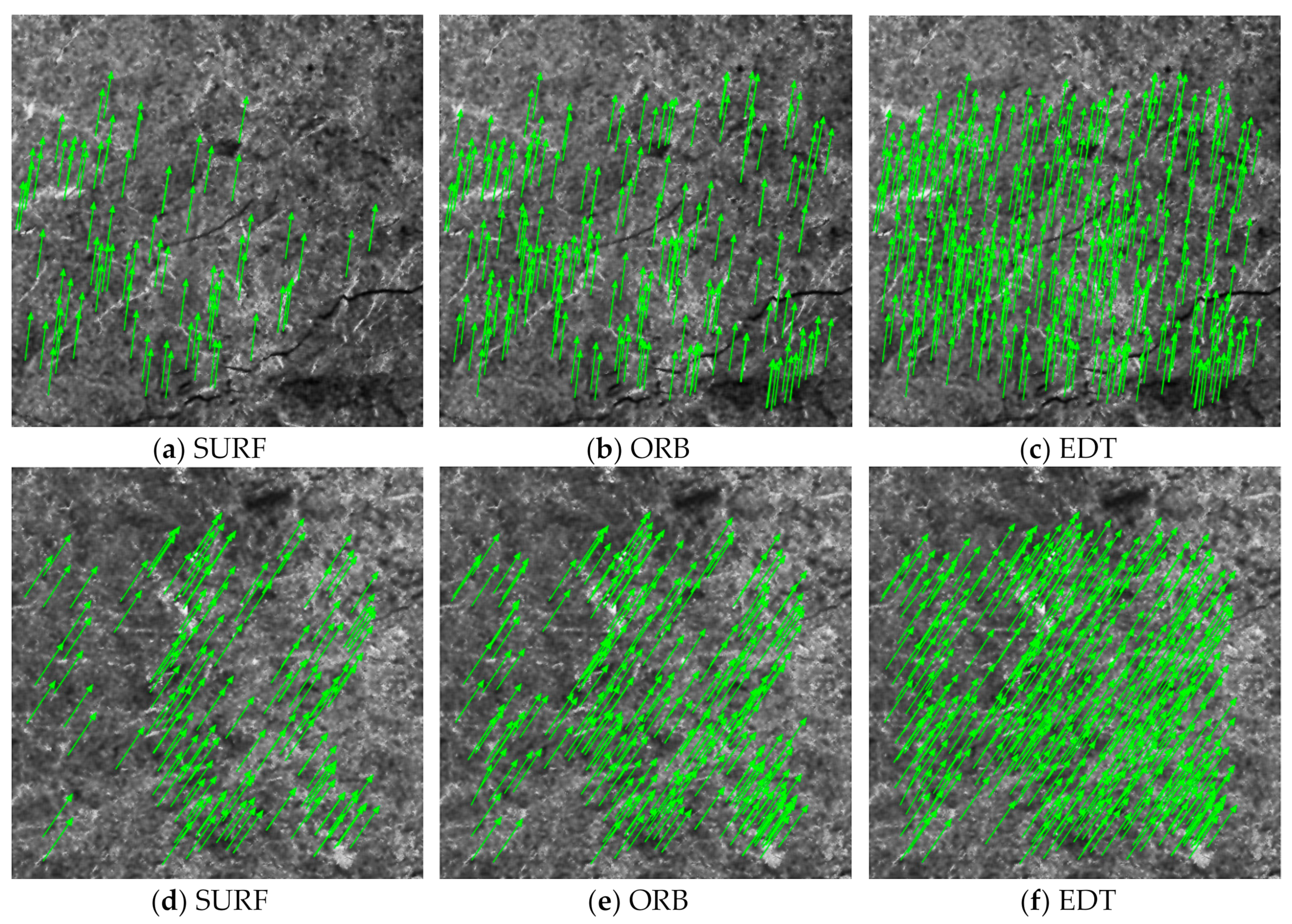
4.3. Comparison with SURF and ORB Method

To evaluate our sea ice drift retrieval method, we compared the result of the ETD method with the SURF [29] and ORB algorithms [41,43] in the two cases described in Figure 1. The SURF algorithm is a novel-scale and rotation-invariant detector and descriptor. This operator solves the disadvantages of SIFT’s high computational complexity, and it approximates or even outperforms previously proposed schemes with respect to repeatability, distinctiveness, and robustness. It can also be computed and compared much faster. The ORB method is a very fast binary descriptor based on BRIEF, which is rotation invariant and resistant to noise. The efficiency has been tested on several real-world applications, including object detection and patch-tracking on a smartphone. The distribution of feature points can be seen from Figure 10. We observed that the SURF feature points extractor showed the most sparse key points, with many gaps and large distances between feature points as shown in Figure 10a. Compared with the SURF method, the ORB method was improved, but there were still a lot of gaps between feature points, as shown in Figure 10b. As evident from Figure 10c, the EDT method performed well in feature space distribution and feature distance compared to the other two methods.

In order to confirm these observations, we used a Voronoi diagram to evaluate the spatial density of feature points. As detailed in Figure 11, the color mapping zone from blue to red indicates that the spatial density varies from high to low. It can be observed that all of the algorithms tended to be deep blue in the center position, and there were only nonblue regions in the marginal region, which was largely due the fact that the target area had drifted away in the second image. As evident in Figure 11, SURF provided local low-density regions and the distribution was irregular. ORB generated relatively regular distribution but still had sparse regions. However, the performance of our method was quite outstanding in all aspects.

Figure 12 illustrates the sea ice drift vectors with three methods. It is evident that the distribution of drift vectors obtained from the SURF and ORB methods were not uniform, and there were a lot of gaps. The number of sea ice drift vectors with our method was two times greater than with SURF or SIFT, and the distribution of sea ice drift vectors was more even. In addition, the gaps between neighbor vectors were noticeably lower.

4.4. Comparison with Adjacent Buoys

In this paper, the IABP (International Arctic Buoy Programme) Buoy dataset was used for verification. This dataset contains the position information (latitude/longitude) of the buoys and the corresponding time information, so we were able to easily calculate the velocity of the buoy for specific time. To evaluate the algorithm performance, we compared our experiment result against the sea ice drift speed obtained by the buoy data. Due to the limited number of buoys, we had to compare the latitude/longitude information of the buoy data and the experimental area and select the nearest buoys for case 1 and case 2 to verify the accuracy of the algorithm. There may be some errors in this verification method, but it was the best evaluation methods we could find at this stage.

The speed of the sea ice drift with our method can be calculated by the following formula:

$$v=\sqrt{d_x^2+d_y^2}\times GSD/(t_2-t_1)$$

(8)

where $GSD$ denotes the ground sample distance, which describes the physical size of one SAR image pixel, and $d_x=x_2-x_1$ and $d_y=y_2-y_1$ is the offset component of sea ice in the horizontal and vertical direction (in pixels), respectively. $(x_1,y_1)$ and $(x_2,y_2)$ are the positions of the targets in the two-scene image at a time $t_1$ and $t_2$, and $(t_2-t_1)$ represents the time interval for monitoring the drift of sea ice.

As shown in

Table 3. Comparison of the average of sea ice drift speed (km/h).

Case	Buoy Speed	SURF	ORB	EDT
1	0.299	0.336	0.325	0.318
2	0.286	0.328	0.316	0.298

, the detective speed was obtained by three algorithms and was consistent with the velocity of the buoy. Compared with the velocity acquired from buoy data, the velocities obtained from the SURF and ORB methods have a large deviation. The ice drift velocity obtained by our method was closest to that of the buoy speed with less deviation.

5. Conclusions

Sea ice drift is one of the most important natural phenomena in the polar region. It has great significance for global climate analysis and waterway planning and presents a potential risk for navigation and other industrial activities. In order to efficiently monitor the sea ice motion, we proposed a novel method with Sentinel-1 SAR images for sea ice drift retrieval. Our sea ice drift algorithm was based on dual-polarization Sequential SAR images and was designed to combine feature tracking and pattern matching arithmetic. It contained several processes, including data preprocessing, feature detection and description, feature matching and fusion, outlier detection and correction, and Enhanced Delaunay Triangulation sea ice tracking with a feature tracking and pattern matching method.

The algorithm application was illustrated on the retrieval of sea ice drift from two pairs of Sentinel-1A SAR images in 2017. First, we compared the performance of feature extraction used by dual polarization, and found the HH polarization was beneficial for sea ice tracking compared to the HV polarization. Compared with the single-polarization image, a combination of the HH and HV polarization extracted more feature points, and the gap between feature points was obviously smaller. Furthermore, it had only a few feature points of closest distance exceeding 40 pixels. Compared to the outlier detection and correction between the Pauta Criterion and Random Sample Consensus (RANSAC) method, the result showed that the confidence interval within (μ − σ, μ + σ) did only remove all of the outliers, but also kept all of the good matching points, which is especially suitable for outlier detection and correction. Finally, we evaluated the algorithm against other feature tracking techniques and adjacent buoys. The results of the experiment provided compelling evidence that our method performed well in feature space distribution and feature distance and had a higher monitor accuracy than the detection from SURF and ORB methods. Then, we validated the accuracy of the retrieval of sea ice drift with the buoy data. We found that our result was consistent with the drift direction of buoy data, and the error was only about 10 m. The study concludes that the performance of our method was quite outstanding with respect to sea ice drift.

This novel method is especially suitable for sea ice drift retrieval. We believe that the method described in our study will provide significant contributions to the retrieval of sea ice drift in the future. Although the algorithm has good favorable effects, it is limited to rigid motion, such as translation and rotation. There might be a failure in achieving nonrigid motion, such as expansion, contraction, and distortion. So, an important question for future studies is the retrieval of sea ice nonrigid motion.

References

1. Darby, D.A.; Ortiz, J.D.; Grosch, C.E.; Lund, S.P. 1500-year cycle in the arctic oscillation identified in holocene arctic sea-ice drift. Nat. Geosci. 2012, 5, 897–900. [Google Scholar] [CrossRef]
2. Girard-Ardhuin, F.; Ezraty, R. Enhanced arctic sea ice drift estimation merging radiometer and scatterometer data. IEEE Trans. Geosci. Remote Sens. 2012, 50, 2639–2648. [Google Scholar] [CrossRef] [Green Version]
3. Meier, W.N.; Dai, M. High-resolution sea-ice motions from amsr-e imagery. Ann. Glaciol. 2006, 44, 352–356. [Google Scholar] [CrossRef] [Green Version]
4. Korosov, A.A.; Rampal, P. A combination of feature tracking and pattern matching with optimal parametrization for sea ice drift retrieval from sar data. Remote Sens. 2017, 9, 258. [Google Scholar] [CrossRef] [Green Version]
5. Griebel, J.; Dierking, W. A method to improve high-resolution sea ice drift retrievals in the presence of deformation zones. Remote Sens. 2017, 9, 718. [Google Scholar] [CrossRef] [Green Version]
6. Kræmer, T.; Johnsen, H.; Brekke, C. Emulating sentinel-1 doppler radial ice drift measurements using envisat asar data. IEEE Trans. Geosci. Remote Sens. 2015, 53, 6407–6418. [Google Scholar] [CrossRef] [Green Version]
7. Barth, A.; Canter, M.; Schaeybroeck, B.V.; Vannitsem, S.; Massonnet, F.; Zunz, V.; Mathiot, P.; Alvera-Azcárate, A.; Beckers, J.M. Assimilation of sea surface temperature, sea ice concentration and sea ice drift in a model of the southern ocean. Ocean Model. 2015, 93, 22–39. [Google Scholar] [CrossRef] [Green Version]
8. Ninnis, R.; Emery, W.; Collins, M. Automated extraction of pack ice motion from advanced very high resolution radiometer imagery. J. Geophys. Res. Ocean. 1986, 91, 10725–10734. [Google Scholar] [CrossRef]
9. Emery, W.; Fowler, C.; Hawkins, J.; Preller, R. Fram strait satellite image-derived ice motions. J. Geophys. Res. Oceans 1991, 96, 4751–4768. [Google Scholar] [CrossRef]
10. Haarpaintner, J. Arctic-wide operational sea ice drift from enhanced-resolution quikscat/seawinds scatterometry and its validation. IEEE Trans. Geosci. Remote Sens. 2005, 44, 102–107. [Google Scholar] [CrossRef]
11. Kaleschke, L.; Lüpkes, C.; Vihma, T.; Haarpaintner, J.; Bochert, A.; Hartmann, J.; Heygster, G. Ssm/i sea ice remote sensing for mesoscale ocean-atmosphere interaction analysis. Can. J. Remote Sens. 2001, 27, 526–537. [Google Scholar] [CrossRef]
12. Zhao, Y.; Liu, A.K.; Long, D.G. Validation of sea ice motion from quikscat with those from ssm/i and buoy. IEEE Trans. Geosci. Remote Sens. 2002, 40, 1241–1246. [Google Scholar] [CrossRef]
13. Gutiérrez, S.; Long, D.G. Optical flow and scale-space theory applied to sea-ice motion estimation in antarctica. In Proceedings of the IGARSS 2003—2003 IEEE International Geoscience and Remote Sensing Symposium, Proceedings (IEEE Cat. No. 03CH37477). Toulouse, France, 21–25 July 2003; pp. 2805–2807. [Google Scholar]
14. Thomas, M.; Geiger, C.A.; Kambhamettu, C. High resolution (400 m) motion characterization of sea ice using ers-1 sar imagery. Cold Reg. Sci. Technol. 2008, 52, 207–223. [Google Scholar] [CrossRef]
15. Linow, S.; Hollands, T.; Dierking, W. An assessment of the reliability of sea-ice motion and deformation retrieval using sar images. Ann. Glaciol. 2015, 56, 229–234. [Google Scholar] [CrossRef] [Green Version]
16. Yu, J.; Yang, Y.; Liu, A.K.; Zhao, Y. Analysis of sea ice motion and deformation in the marginal ice zone of the bering sea using sar data. Int. J. Remote Sens. 2009, 30, 3603–3611. [Google Scholar] [CrossRef]
17. Liu, H.; Li, X.-M.; Guo, H. The dynamic processes of sea ice on the east coast of antarctica—a case study based on spaceborne synthetic aperture radar data from terrasar-x. IEEE J. Sel. Top. Appl. Earth Obs. Remote Sens. 2015, 9, 1187–1198. [Google Scholar] [CrossRef]
18. Johansson, A.M.; Berg, A. Agreement and complementarity of sea ice drift products. IEEE J. Sel. Top. Appl. Earth Obs. Remote Sens. 2017, 9, 369–380. [Google Scholar] [CrossRef]
19. Fowler, C.; Emery, W.J.; Maslanik, J. Satellite-derived evolution of arctic sea ice age: October 1978 to march 2003. IEEE Geosci. Remote Sens. Lett. 2004, 1, 71–74. [Google Scholar] [CrossRef]
20. Fowler, C.; Emery, W.; Tschudi, M. Polar Pathfinder Daily 25 km Ease-Grid Sea Ice Motion Vectors, Version 2; National Snow and Ice Data Cent: Boulder, CO, USA, 2013. [Google Scholar]
21. Lee, S.M.; Sohn, B.J.; Kim, S.J. Differentiating between first-year and multiyear sea ice in the arctic using microwave-retrieved ice emissivities. J. Geophys. Res. Atmos. 2017, 122, 5097–5112. [Google Scholar] [CrossRef]
22. Petrou, Z.I.; Tian, Y. High-resolution sea ice motion estimation with optical flow using satellite spectroradiometer data. IEEE Trans. Geosci. Remote Sens. 2016, 55, 1339–1350. [Google Scholar] [CrossRef]
23. Gao, J.; Lythe, M. The maximum cross-correlation approach to detecting translational motions from sequential remote-sensing images. Comput. Geosci. 1996, 22, 525–534. [Google Scholar] [CrossRef]
24. Berg, A.; Eriksson, L.E. Investigation of a hybrid algorithm for sea ice drift measurements using synthetic aperture radar images. IEEE Trans. Geosci. Remote Sens. 2014, 52, 5023–5033. [Google Scholar] [CrossRef] [Green Version]
25. Reddy, B.S.; Chatterji, B.N. An fft-based technique for translation, rotation, and scale-invariant image registration. IEEE Trans. Image Process. 1996, 5, 1266–1271. [Google Scholar] [CrossRef] [PubMed] [Green Version]
26. Komarov, A.S.; Barber, D.G. Sea ice motion tracking from sequential dual-polarization radarsat-2 images. IEEE Trans. Geosci. Remote Sens. 2014, 52, 121–136. [Google Scholar] [CrossRef]
27. Lowe, D.G. Distinctive image features from scale-invariant keypoints. Int. J. Comput. Vis. 2004, 60, 91–110. [Google Scholar] [CrossRef]
28. Perona, P.; Malik, J. Scale-space and edge detection using anisotropic diffusion. IEEE Trans. Pattern Anal. Mach. Intell. 1990, 12, 629–639. [Google Scholar] [CrossRef] [Green Version]
29. Bay, H.; Ess, A.; Tuytelaars, T.; Gool, L.V. Speeded-up robust features (surf). Comput. Vis. Image Underst. 2008, 110, 346–359. [Google Scholar] [CrossRef]
30. Muckenhuber, S.; Korosov, A.A.; Sandven, S. Open-source feature-tracking algorithm for sea ice drift retrieval from sentinel-1 sar imagery. Cryosphere 2016, 10, 913–925. [Google Scholar] [CrossRef] [Green Version]
31. Daida, J.; Samadani, R.; Vesecky, J.F. Object-oriented feature-tracking algorithms for sar image of the marginal ice zone. IEEE Trans. Geosci. Remote Sens. 1990, 28, 573–589. [Google Scholar] [CrossRef]
32. Giles, A.B.; Massom, R.A.; Heil, P.; Hyland, G. Semi-automated feature-tracking of east antarctic sea ice from envisat asar imagery. Remote Sens. Environ. 2011, 115, 2267–2276. [Google Scholar] [CrossRef]
33. Mcconnell, R.; Kwok, R.; Curlander, J.C.; Kober, W.; Pang, S.S. Ψ-s correlation and dynamic time warping: Two methods for tracking ice floes in sar images. IEEE Trans. Geosci. Remote Sens. 1991, 29, 1004–1012. [Google Scholar] [CrossRef] [Green Version]
34. Demchev, D.; Volkov, V.; Kazakov, E.; Alcantarilla, P.F.; Sandven, S.; Khmeleva, V. Sea ice drift tracking from sequential sar images using accelerated-kaze features. IEEE Trans. Geosci. Remote Sens. 2017, 55, 5174–5184. [Google Scholar] [CrossRef]
35. Wang, P.; Zhang, H.; Patel, V.M. Sar image despeckling using a convolutional neural network. IEEE Signal Process. Lett. 2017, 24, 1763–1767. [Google Scholar] [CrossRef] [Green Version]
36. Parrilli, S.; Poderico, M.; Angelino, C.V.; Verdoliva, L. A nonlocal sar image denoising algorithm based on llmmse wavelet shrinkage. IEEE Trans. Geosci. Remote Sens. 2012, 50, 606–616. [Google Scholar] [CrossRef]
37. Rebay, S. Efficient unstructured mesh generation by means of delaunay triangulation and bowyer-watson algorithm. J. Comput. Phys. 1993, 106, 125–138. [Google Scholar] [CrossRef]
38. Lee, D.-T.; Lin, A.K. Generalized delaunay triangulation for planar graphs. Discret. Comput. Geom. 1986, 1, 201–217. [Google Scholar] [CrossRef] [Green Version]
39. Lertrattanapanich, S.; Bose, N.K. High resolution image formation from low resolution frames using delaunay triangulation. IEEE Trans. Image Process. 2002, 11, 1427–1441. [Google Scholar] [CrossRef]
40. Shen, C.; Bao, X.; Tan, J.; Liu, S.; Liu, Z. Two noise-robust axial scanning multi-image phase retrieval algorithms based on pauta criterion and smoothness constraint. Opt. Express 2017, 25, 16235–16249. [Google Scholar] [CrossRef]
41. Muckenhuber, S.; Sandven, S. Open-source sea ice drift algorithm for sentinel-1 sar imagery using a combination of feature-tracking and pattern-matching. Cryosphere Discuss. 2017, 11, 1835–1850. [Google Scholar] [CrossRef] [Green Version]
42. Fischler, M.A.; Bolles, R.C. Random sample consensus: A paradigm for model fitting with applications to image analysis and automated cartography. Commun. ACM 1987, 24, 726–740. [Google Scholar]
43. Rublee, E.; Rabaud, V.; Konolige, K.; Bradski, G. Orb: An efficient alternative to sift or surf. In Proceedings of the 2011 International Conference on Computer Vision, Barcelona, Spain, 6–13 November 2011; pp. 2564–2571. [Google Scholar]
Figure 1. Location of the study area and the Synthetic Aperture Radar (SAR) data for the sea ice drift retrieval.
Remotesensing 12 00581 g001
Figure 2. Flowchart of the sea ice drift retrieval algorithm.
Remotesensing 12 00581 g002
Figure 3. (a) Original SAR image, of size 512 × 512 pixels, we selected a row of SAR image data with a red line to compare the spatial luminance profile changes. (b) Filtered results with the SAR block-matching 3-D (SAR-BM3D) method. (c) Filtered results with the image despeckling convolutional neural network (ID-CNN) method. Spatial luminance profile changes at the red row of the SAR image: (d) Unfiltered SAR image, (e) filtered via SAR-BM3D method, and (f) filtered via ID-CNN method.
Remotesensing 12 00581 g003aRemotesensing 12 00581 g003b
Figure 4. Constructed a triangular network by the Delaunay Triangulation algorithm.
Remotesensing 12 00581 g004
Figure 5. Combination of feature tracking and pattern matching algorithm.
Remotesensing 12 00581 g005
Figure 6. Illustration of the maximum cross-correlation (MCC) method. (a) First image. (b) Second image. (c) The cross-correlation matrix between sub-image with a green empty square and the sub-image with a yellow empty square.
Remotesensing 12 00581 g006
Figure 7. Comparison of successfully matched key points from (a) HH polarization, (b) HV polarization, and (c) HH + HV polarization. The key points are extracted from case 1.
Remotesensing 12 00581 g007
Figure 8. Boxplot of distances between neighbor vector, tracked with HH, HV, and HH + HV polarization for case 1.
Remotesensing 12 00581 g008
Figure 9. Comparing the performance of the outlier removal with the horizontal displacements by different methods for case 2. The x-axis represents the simulated start position ×1, and the y-axis represents the end position ×2. (a) Original image. (b) Result of (μ − 3σ, μ + 3σ). (c) Result of (μ − 2σ, μ + 2σ). (d) Result of (μ − σ, μ + σ) (e). Result of Random Sample Consensus (RANSAC). Red points are identified as outliers.
Remotesensing 12 00581 g009
Figure 10. The results of feature points tracking with SURF, ORB, and EDT methods. Results of (a) SURF, (b) ORB and (c) EDT methods for case 1. Results of (d) SURF, (e) ORB and (f) EDT methods for case 2.
Remotesensing 12 00581 g010
Figure 11. Spatial Density of feature points tracking with the SURF, ORB, and EDT methods. Results of (a) SURF, (b) ORB and (c) EDT methods for case 1. Results of (d) SURF, (e) ORB and (f) EDT methods for case 2.
Remotesensing 12 00581 g011aRemotesensing 12 00581 g011b
Figure 12. Visualization of sea ice drift vectors with the SURF, ORB, and EDT methods. Results of (a) SURF, (b) ORB and (c) EDT methods for case 1. Results of (d) SURF, (e) ORB and (f) EDT methods for case 2.
Remotesensing 12 00581 g012