Article

Sliding Time Master Digital Image Correlation Analyses of CubeSat Images for landslide Monitoring: The Rattlesnake Hills Landslide (USA)

1
Department of Earth Sciences, Sapienza University of Rome, Piazzale Aldo Moro 5, 00185 Rome, Italy
2
NHAZCA S.r.l., spin-off Sapienza University of Rome, Via Vittorio Bachelet, 12, 00185 Rome, Italy
3
ACEA Elabori S.p.A., Engineering Geology Division, Via Vitorchiano 165, 00189 Rome, Italy
*
Author to whom correspondence should be addressed.
Submission received: 30 December 2019 / Revised: 26 January 2020 / Accepted: 3 February 2020 / Published: 11 February 2020
(This article belongs to the Special Issue Remote Sensing in Engineering Geology)

Abstract

:
Landslide monitoring is a global challenge that can take strong advantage from opportunities offered by Earth Observation (EO). The increasing availability of constellations of small satellites (e.g., CubeSats) is allowing the collection of satellite images at an incredible revisit time (daily) and good spatial resolution. Furthermore, this trend is expected to grow rapidly in the next few years. In order to explore the potential of using a long stack of images for improving the measurement of ground displacement, we developed a new procedure called STMDA (Slide Time Master Digital image correlation Analyses) that we applied to one year long stack of PlanetScope images for back analyzing the displacement pattern of the Rattlesnake Hills landslide occurred between the 2017 and 2018 in the Washington State (USA). Displacement maps and time-series of displacement of different portions of the landslide was derived, measuring velocity up to 0.5 m/week, i.e., very similar to velocities available in literature. Furthermore, STMDA showed also a good potential in denoising the time-series of displacement at the whole scale with respect to the application of standard DIC methods, thus providing displacement precision up to 0.01 pixels.

Graphical Abstract

1. Introduction

Space-borne Earth Observation (EO) is one of the most valuable solutions for Earth’s surface spatial and temporal monitoring, with fundamental socio-economic benefits [1,2,3,4]. Since the early stage, EO has been considered a promising tool for better managing and preventing natural hazards due, especially, to the unique capability of looking simultaneously at large areas [5,6]. However, some evident limitations for monitoring purposes are connected with temporal and spatial resolution of the images [7,8,9].
Several successful applications of landslide mapping after extreme events such as rainfalls or earthquakes exists [10,11,12,13] and, especially in the last two decades, also monitoring small displacements caused by landslides using Synthetic Aperture Radar Interferometry has been possible [14,15,16,17]. In the last years, new image processing tools were developed and examples of landslide displacement monitoring, based on optical satellite images are available [7,12,18,19,20,21]. However, only few authors attempted to derive time-series of displacement using long stack of satellite optical images, thus demonstrating the potential of such an approach to derive time of series of displacement along the plane normal to the line of sight with a sub-pixel accuracy [6,20,22,23,24].
The most common optical satellite missions (e.g., QuickBird, SPOT, LANDSAT, Sentinel-2, WorldView, Pléiades, just to mention few of them) are characterized by spatial resolution ranging between 0.3 and 30 m and a revisit time of some days [25,26,27], therefore, they are not fully adequate to detect landslides at a spatial and temporal scale suitable for continuous monitoring. However, as stated in [4,28], the fusion of images collected by different optical satellite sensors has certainly increased the opportunities for cloud-free surface investigation, thus allowing also a general improvement of the temporal resolution.
In the last few years, EO has been affected by an astonishing sensor and platform development and improvement, thanks to small satellites. According to [27,29,30], among the main features of these satellites, properly named CubeSats, there are: (i) the general small size and weight (a single-unit of CubeSat normally measures 10 × 10 × 11 cm and typically weights less than 1.5 kg), (ii) high geometric resolution (~3–5 m/pixel) and (iii) daily/near-daily revisit time. CubeSats represent a cost-effective EO strategy, allowing unique chances for a wide variety of application fields [8,31].
Planet Labs Inc. has recently made available a large constellation (> 130 units) of optical 3-U CubeSats (10 × 10 × 30 cm), also called PlanetScope or, more commonly, “Doves” [27,30,32,33,34]. With an average orbit height of about 475 km a.s.l., the main CCD array sensor is able to collect images of 7000 × 2000 pixels, with a footprint of approximately 24 × 8 km2. Each Doves collects one image/second along his orbit with a slight overlapping between consecutive scenes. In this way, taking advantage of the whole constellation, images at a daily sampling rate are achievable, thus allowing to obtain long stacks of multi-temporal images in a short period [8,34].
At present, only few authors used “Doves” images for the assessment of landslides [35] or earthquakes-induced displacement [8], while, no attempts of deriving time-series of displacements of landslides using stack of Doves images processed by Digital Image Correlation (DIC) are available in literature.
Recently, different authors presented interesting results derived from the application of DIC analysis on a stack of satellite images for landslide displacement monitoring [22,24]. Specifically, they developed a workflow adapted for satellite optical images with the aim of achieving the best signal/noise ratio by taking advantage of the data redundancy. In this paper, we developed and applied a similar processing procedure for the analyses of a long stack of Planet Scope Images aiming at providing time-series of displacement. The results derived from the application of our processing procedure, named STMDA (Sliding Time Master DIC Analysis), on a large landslide occurred in the Rattlesnake Hills (Washington State, USA) (Figure 1), is herein presented. The Rattlesnake Hills landslide was selected as a nice example of a recent active landslide (i.e., allowing the availability of a good stack of Doves images) characterized by a relatively large size and amount of surface deformation. Furthermore, the availability of an extensive field monitoring network was a key factor for the validation of the results achieved in our study.

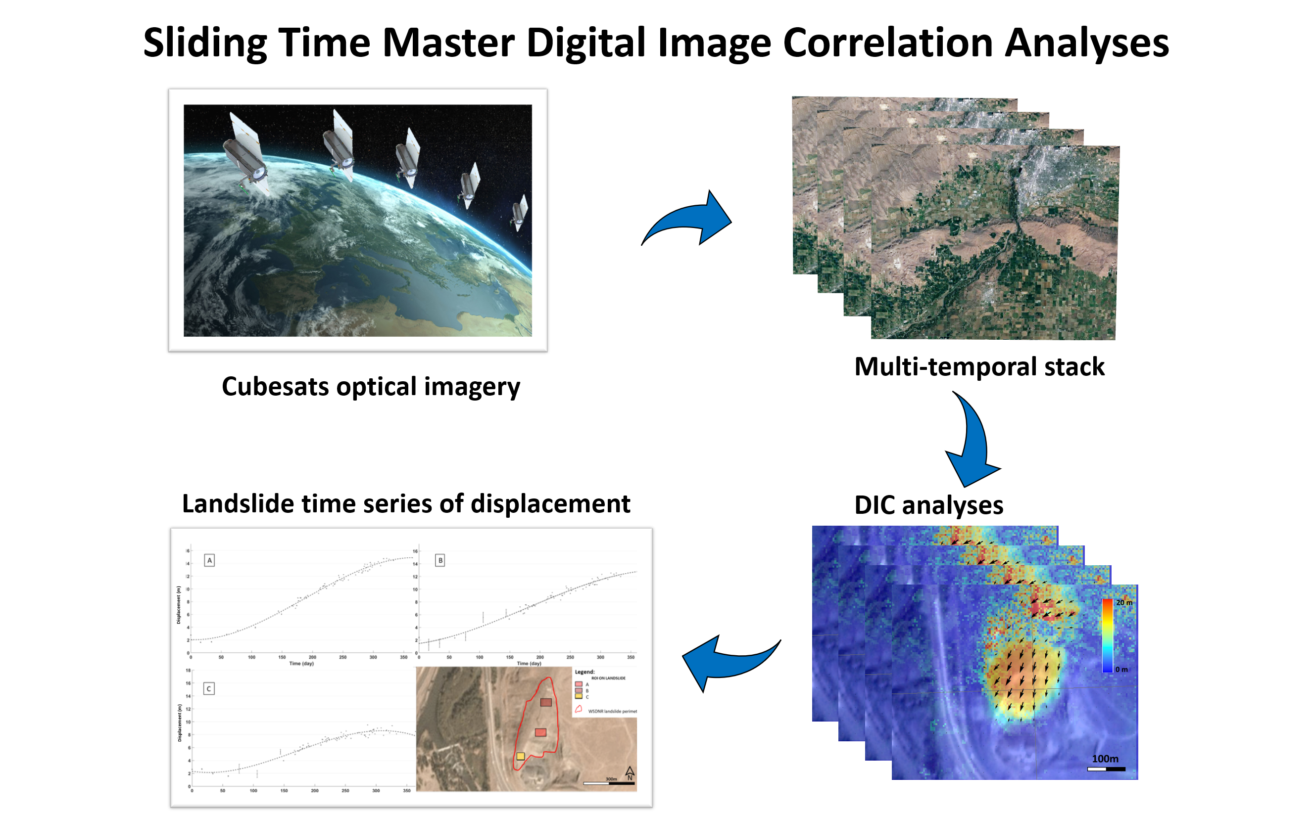
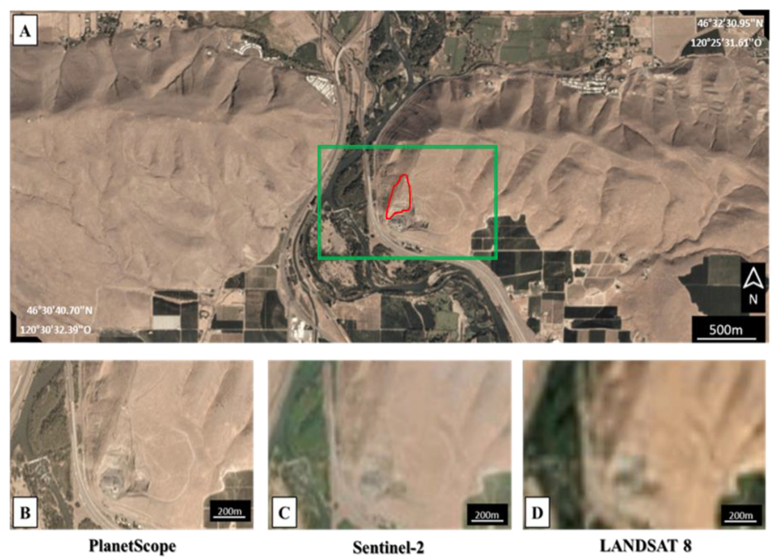
2. The Rattlesnake Hills Landslide

The Rattlesnake Hills landslide is located near Union Gap, about 10 km southern of the city of Yakima (WA, USA). According to [36,37,38] and the Washington State Department of Natural Resources, the landslide was activated in October 2017, when tension cracks were observed along the North side of the AK Anderson quarry managed by Columbia Asphalt and Gravel, Inc. The slide involved up to 4 million m3 volume, affecting about 8*104 m2 of the hillside, moving South toward the quarry (Figure 2). The slope instability process has been controlled by sedimentary and tectonic features, which lead to a movement along a weak 10–15 degrees inclined sedimentary interbed within basalt flow sequence [36,37,38].
The Rattlesnake Hills landslide has been classified as a translational slide, significantly disjointed in the upper part as evidenced by huge tension cracks in continuous expansion [36,38]. Based on [37], the recent quarrying activities at the toe of the landslide may have weakened the whole slope system, thus activating a “wedge” of rock that in the first months of 2018 reached a velocity in the order of 0.5 m/week.
Following the landslide triggering, different kinds of contact and remote sensing monitoring systems, such as GPS (Global Position System), seismometers, robotic total stations, multi-temporal UAV (Unmanned Aerial Vehicles) photogrammetric and TLS (Terrestrial Laser Scanner) surveys, TInSAR (Terrestrial Interferometric Synthetic Aperture Radar) and 24-h webcam have been deployed [36,37,38,39]. According to [37] and [38], in situ displacement measurements confirmed that the Rattlesnake Hills landslide has moved toward S-SW direction, along the 10–15° dipping rupture surface discussed above. The extensive monitoring network allowed to measure the strong displacement trend as well as the landslide bounding features, direction and inclinations of the tension cracks. The landslide showed an accelerating trend between October 2017 and January 2018 with the highest displacement velocities showed in the central portion of the landslide mass in the period mid December 2017 to mid-January 2018 (with a peak of 56 cm/week horizontal velocity). The upper part of the landslide showed, in the monitoring period, velocities lower than the central portion (average horizontal velocity of about 12 cm/week) with a higher vertical component that caused large ground cracks, due to the stretching action. The lowest velocity was recorded in valley wedge mass. According to [36] and [38], this strain behavior can be explained by assuming the stabilizing role of the valley portion on the moving volume, and the subsidence trends of upper portion.

3. Material and methods

Thanks to the Planet Labs’ image dissemination policy for research and education purposes, it has been possible to access a whole stack of 3 m/pixel PlanetScope analytic (ortho-rectified) images [34], over the Rattlesnake Hills landslide area. In total, 63 images of the 139 available have been selected for their low cloud coverage (maximum 20%) over a period of 12 months (i.e., from mid-September 2017 till mid-September 2018) (Figure 3).
Figure 3 shows also the images collected in the same area and in the same time-frame by Sentinel 2 and Landsat 8 satellite missions.

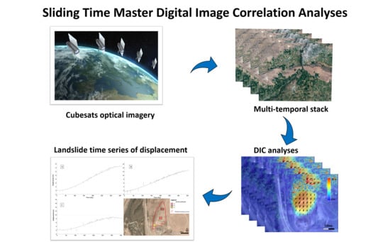
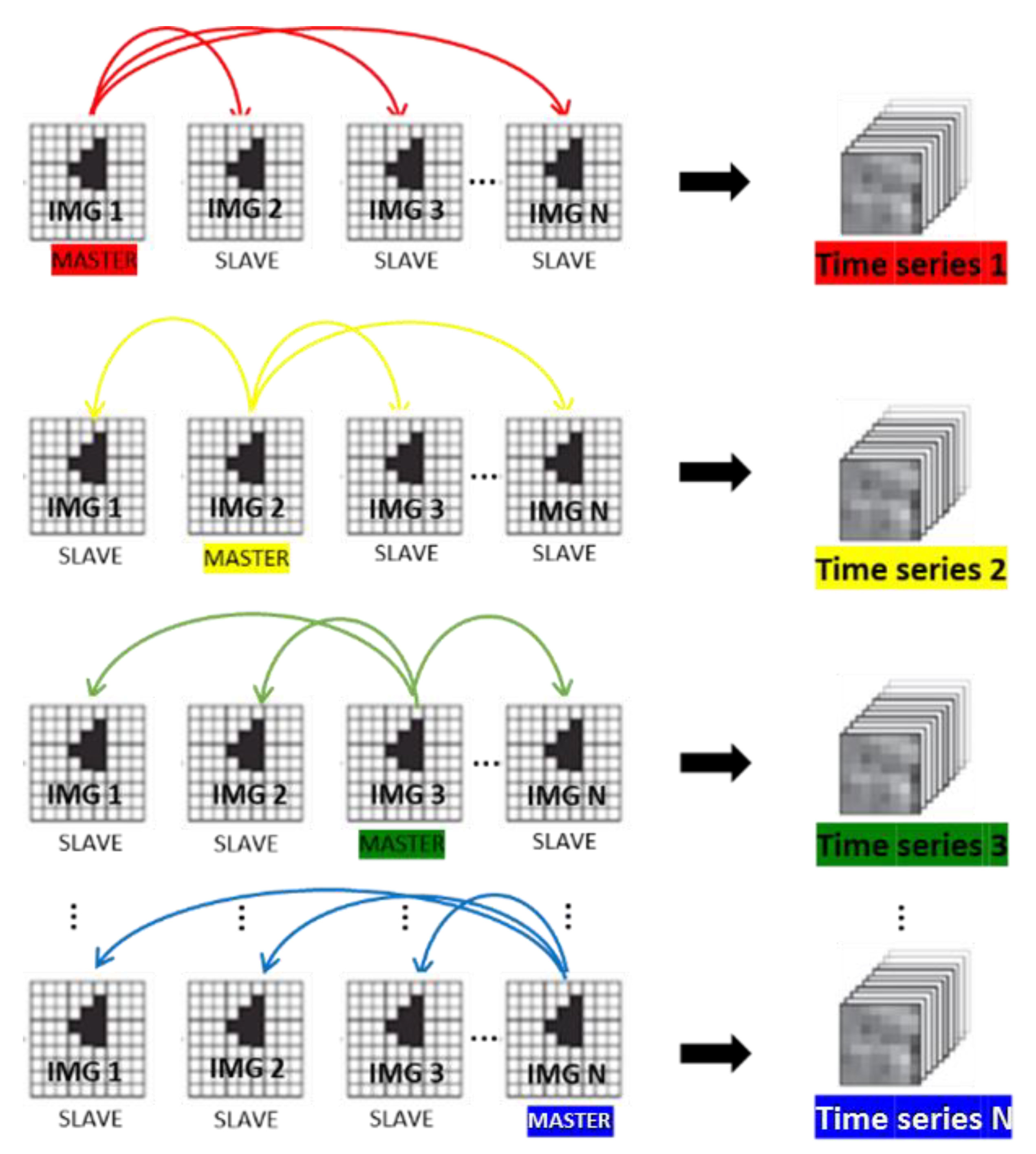
Sliding Time Master DIC Analyses (STMDA)

The first analyses of the available PlanetScope images was performed by the processing chain proposed by [18]. Specifically, the first two steps are included in the orthorectification and georeferencing elaboration made by Planet [8], while the third step (i.e., the correlation phase) is performed using an advanced stacking correlation scheme, similar to the one developed by [22,24] and extensively described below. Advanced stacking DIC analysis allowed to achieve, for each pixel, the value of displacement along the N-S and E-W directions and the correlation coefficient (i.e., an estimation of the “cross-correlation quality”), with an increase of signal to noise ratio [6,21,22,24]. Specifically, DIC analysis is here applied to all the possible image pairs of the selected dataset with a progressive correlation scheme showed in Figure 4. The progressive correlation scheme is applied iteratively using all the available images as the master, thus achieving a fully redundant stack of correlation maps characterized by different time-spans.
The DIC analyses have been carried out by the open source plug-in of ENVI®, named COSI-Corr (Co-registration of Optically Sensed Images and Correlation) that is based on a sub-pixel image correlation algorithm developed by [18] and [40]. COSI-Corr is a DIC software implemented in the IDL language for geoscience application, with a specific focus on geomorphological surface dynamics monitoring [41]. Specifically, all the correlation maps were obtained using the frequency correlation option available in COSI-Corr that consists in an iterative process made of a preliminary estimation of the pixel wise displacement between two patches followed by a final correlation to retrieve the subpixel displacement. Due to the huge number of image pairs, a batch correlation was performed by using a parameters selection scheme representing the best compromise between computational time and accuracy in displacement estimations for the Rattlesnake Hills case study. Correlation maps of about 6 m/pixel resolution resulting from original pixel size of 3 m, was investigated with a sliding window of 128 pixels and a correlation step size of 2 pixels. More than 3900 correlation maps have been achieved by the fully redundant correlation scheme of the 63 selected images. At this regard, it is worth to note that DIC displacement values are computed along the directions corresponding to the normal plane to the line of sight. For that reason, by using orthorectified images, we got displacements only along the horizontal directions (i.e., N-S and E-W directions).
The output of the above correlation process for each pixel and each component here defined as the “redundant correlation matrix” is represented by a number of time-series of displacement equal to the number of the master images (i.e., all the selected images) achieved by an inversion procedure similar to the one presented in [22,24]. The inversion allows to provide all the time-series (derived from the different master images) a “zero-displacement value” corresponding to time “zero” (i.e., the date of the oldest image of the stack).
For the analyses of the “redundant correlation matrix” an ad hoc processing chain was developed in MATLAB v. R2018a. The first step of the STMDA approach consists in the computation of the average displacement values for all the time-series available at each time instant. This procedure was iterated for each pixel, thus producing the denoised time-displacement stack that can be used for the time-series of displacement. Furthermore, the correlation coefficient has been used as a filtering tool by discarding values with Correlation Coefficient (CC) < 0.8. This procedure allows to denoising the displacement results, thus increasing the robustness of the measurement [22,24].
However, the above described procedure cannot solve the errors contribution due to localized changes in radiometric content that can occur for several causes at the scale of a single pixel, especially for spatially heterogeneous processes, like landslides. To this aim, an approach based on the analysis of Region-Of-Interest (ROI) made of adjacent pixels with a similar displacement behavior was developed. By analyzing the displacement values of each pixel at each time interval, from the redundant correlation matrix we derive, for each time instant and each time-series, one displacement value (for each component) that is statistically representative of the selected ROI (see at Figure 5).
The measurements dispersion relative to the selected ROI in the time/displacement graph is reported in Figure 6A.
In order to remove the noisy time-series of displacement and find the best fitting between the derived data, we developed an algorithm for identifying the best I, II or III order polynomial functions that maximize the R2 coefficient and fitting, at the same time, the maximum number of time-series.
Then, the displacement values from the redundant correlation matrix that do not fit the characteristics found after the above processing step are discarded (Figure 6B).
Following the above procedure, it is now possible to derive a new polynomial regression of the averaged time-series obtained from the filtered redundant correlation matrix, thus achieving the best results in computing the surface displacement in time. At this stage, the standard deviation of the instantaneous displacement resulting from the above described filtering procedure, can be assumed as the precision of the STMDA measurements at each time frame.
Residual error estimation of the STMDA procedure is then carried out analyzing ROIs not affected by displacement (i.e., area outside the landslide not affected by ground movement). In this area, we can assume that all the measured displacement values are due to systematic and random error contribution, hence, the average displacement values should be very close to zero and the dispersion of the measurements is representative of the errors.
With the aim of deriving the one-year long Rattlesnake Hills landslide kinematic history (September 2017 to September 2018) we applied the above described STMDA method to the selected stack of PlanetScope images, by identifying some ROIs that could describe the behavior of specific portions of the moving mass [39]. Specifically, three ROIs have been built on the landslide area with a medium size of about 100 pixels (corresponding to about 6400 m2) and four ROIs outside the landslide area (i.e., stable ground) with a medium size of 120 pixels (corresponding to about 7600 m2), for the error estimation. For each ROI on the landslide area the time-series of displacement are derived, while in the ROIs outside the landslide (stable areas), we performed a statistical analysis of displacement data for error estimations.

4. Results

By applying the STMDA processing method to the available stack of PlanetScope images, the multi-temporal horizontal displacements pattern of the Rattlesnake Hills landslide between September 2017 and September 2018 was achieved (Figure 7). The displacement vector field and the whole landslide boundary are consistent with the in situ observations from the WSDNR and others [36,37,38,39].
In Figure 7 the heterogeneous spatial and magnitude distribution of the horizontal deformations can be observed. The highest deformation values are localized in the central-southern part of the landslide, but the highest local values are measured in the northern portion where the higher noise is also visible.
Time-series of displacement has been derived on the three ROIs located inside the landslide boundary showed in Figure 8. Specifically, the maximum computed surface deformation during the monitoring period is between 15 and 16 m in the ROI A and B, while is about 9 m in ROI C. In terms of temporal evolution, it is quite evident an acceleration phase in the first 200 days (corresponding to the period Sept. 2017 to March 2018) and, following, a decelerating phase (April to September 2018). These results are in line with the in situ data reported in [36,37,38,39]. The maximum velocity of about 0.5 m/week was reached in the period mid-February to March 2018 on ROI A and B, while a maximum velocity of about 0.2 m/week is reached in ROI C in March.
Looking at the error bars, we can observe two main evidences: 1) in the first 150 days the length of error bars is larger than in the following phase in all the ROIs; 2) there is a difference in the mean length of error bars between different areas (e.g., in ROI_A the error bars are smaller than in ROI_B and ROI_C). The average value of the error bars, even if slightly different for each ROI, is on the order of 0.01 m.
It is worth to note that fracturing processes, tilting movements, vegetation changes, and other changes on the ground surface can generate errors on the correlation process. For example, ROI_B is characterized by lower precision as it corresponds to the upper part of the landslide where extensive fractures were observed, as demonstrated also by the decrease of correlation coefficient map showed in Figure 9.
Figure 10 reports the noise estimation measurements for the entire period of analysis on the ROI D, E and F (located in areas not affected by the landslide). For all these ROIs, the red line (close to zero) represents the average displacement values in the time domain.
Systematic error caused by the DIC processing tool (i.e., COSI-Corr) was also estimated by the pixelwise subtraction of displacements obtained from homologous image pairs (i.e., 1 vs. 2 and 2 vs. 1, 15 vs. 54 and 54 vs. 15, and so on), thus achieving differences in the order of 0.006 m.

5. Discussions

With the purpose of investigating the potential of using long stack of PlanetScope images for landslide monitoring purposes, we developed an original processing procedure called STMDA that was tested on the Rattlesnake Hills landslide. Figure 11 shows the quality improvement in the landslide displacement mapping using the STMDA stacking procedure with respect to standard DIC analysis (that compares a single couple of images), without applying any radiometric correction to the original images. This is evident in the northern sector of landslide that was characterized by the occurrence of ground cracks, thus causing a significant reduction of the correlation coefficient (Figure 9).
However, residual noise is present also in images A, B and C, mainly due by ground cracks caused by vertical movements (reported in [36,37,38,39]), that cannot be detected by DIC analyses (Figure 9).
In Figure 12, three time-series of displacement corresponding to (i) a single pixel, (ii) average of pixels in ROI B and (iii) results on ROI B achieved from the application of the complete STMDA procedure, are compared. The improvement in the displacement measurement performances using procedure (ii) and, especially, procedure (iii) (i.e., STMDA) is quite evident. The differences are probably due to the radiometric variations induced by the clouds and land cover coverage (especially in the images acquired in the winter season), that in a future perspective, could be partially solved by radiometric corrections applied to the original images.
Time-series derived by the STMDA procedure on the three ROIs located in the landslide area (Figure 10) revealed a whole activation/resting loop of the landslide with an initial acceleration phase (from October 2017 to April 2018) and the consequent deceleration phase (from May to September 2018) (Figure 8), thus showing the overall landslide surface kinematic pattern in the spatial and temporal domains. Specifically, the Rattlesnake Hills landslide showed different displacement magnitude with the lower values measured in the southern part (ROI_C), as confirmed by field measurements [36,38].
The increasing presence of fractures on some portions of the landslide surface represents the most important source of error for the DIC analyses in addition to the presence of snow in the winter season and lighting changes due to different sunlight incidence during the year. However, the STMDA procedure allowed us to mitigate these sources of error, whose residual contribution is described by the error bars showing, as one can expect, higher values during the winter season (Figure 8).
Precision estimation has been performed by using the mean value of the error bars for each time in the diagrams presented in Figure 8. In such a way, it has been possible to achieve, for the ROI_A (located in correspondence of the GPS point characterized by the higher movement) a value of 0.01 m (i.e., less than 0.01 pixels), that is one order of magnitude lower than the results of similar studies available in the scientific literature [6,9,22].
The accuracy of displacement achieved by the STMDA procedure using the above described stack of PlanetScope images has been estimated by the comparison with traditional ground monitoring data available from literature (mainly achieved by total stations and GNSS) [38]. The comparison was performed on the ROI_A by sub-sampling the STMDA time-series in order to make the data comparable with the monthly displacement velocity data available from literature [36,38]. Results of the comparison (Figure 13) show the good correspondence between the displacement values with a few exceptions in the winter season and in September 2018. The general trend of displacement over time is very similar (1.48 cm/day average difference) while, as expected, the absolute values are under-estimated due to the neglection of the vertical component and the spatial average of the STMDA method. These results shed light to one of the limitations of the STMDA procedure, i.e., the capability of measuring displacement only along the plane normal to the line of sight that makes the procedure more effective for horizontal movements than for vertical movements if satellite images acquired with a Nadir view are used. However, we must point out that the STMDA procedure can be applied also to aerial or ground based images, that, having a different line of sight, could allow to measure also vertical movements.
DIC techniques are more popular for lab application but, in the last years, some authors presented interesting results also on natural environments, such as landslides, using a variety of optical sensors [6,9,12,22]. Staking DIC methods, like the STMDA procedure herein presented, have the potential to furtherly increase the capability of this technique taking advantage of a huge number of data with a high revisit time, in order to reduce the source of noise [6,20,21,22,24]. The STMDA procedure based on satellite optical images is complementary to other satellite-based displacement monitoring techniques like Advanced Interferometric Synthetic Aperture Radar (A-DInSAR). A-DInSAR is able to measure movement along the Line of Sight (LOS) direction, providing best performance for vertical movements. However, it is worth to note that A-DInSAR monitoring of the Rattlesnake Hills landslide could have been affected by phase ambiguity problems, due to the high displacement rate. At this regard, it is worth mentioning that A-DInSAR and STMDA are complementary also in terms of displacement velocities. As a matter of fact, considering the classification of Cruden and Varnes [42] A-DInSAR is effective only for extremely slow and very slow landslides, while STMDA is effective for very slow to moderate landslides. Nevertheless, in the perspective of a widespread application of both A-DInSAR and STMDA techniques we cannot forget the main limitations related to the land cover, such as vegetation and snow.

6. Conclusions

This paper demonstrates the potential of the high temporal frequency satellite optical constellations (in this specific case PlanetScope nanosatellite) for landslide monitoring using the herein proposed Sliding Time Master Digital image correlation Analyses (STMDA) processing method. It has been possible to identify and measure the Rattlesnake Hills landslide kinematic behavior between September 2017 and September 2018, achieving a very good fitting with the displacement data collected by local authorities during multi-temporal field surveys. Precision of measurements are up to 1/100 of the pixel size (3 m in this case), that is one order of magnitude higher than those achieved by other authors using ground based, satellite and aerial optical imagery with traditional DIC approaches. The accuracy estimation remarks small differences (in the order of 0.01 m/day) between the velocity achieved using the herein proposed method and the results from in situ measurements, thus opening incredible perspective for systematic satellite-based landslide monitoring at global level. In addition to landslides, STMDA procedure applied to CubeSats images can be useful for other surface displacement processes like glaciers and earthquakes and it is not affected by problems related to high displacement rate as it occurs with A-DInSAR. However, as for any other remote sensing satellite-based displacement monitoring technique, some drawbacks that can affect the STMDA monitoring results must be considered like the vegetation and land cover and the slope inclination. Nevertheless, STMDA has the potential to be applied also to images acquired by others source such as, aerial and ground based sensors, thus allowing to solve most of the above described issues.

Author Contributions

Conceptualization, P.M.; Data curation, R.M., P.C.; Formal analysis, R.M., P.C.; Investigation, R.M.; Methodology, R.M., P.M., P.C.; Resources, P.M., R.M., P.C.; Software, R.M.; Supervision, P.M.; Validation, R.M., P.M.; Visualization, R.M.; Writing—original draft, R.M., P.C.; Writing—review & editing, P.M., P.C. All authors have read and agreed to the published version of the manuscript.

Funding

This research received no external funding.

Acknowledgments

Planet Lab Inc. for providing free access to Planet Scope Images under the Planet’s Education and Research Program.

Conflicts of Interest

The authors declare no conflict of interest.

References

  1. Mantov, F.; Soeters, R.; Van Wasten, C.J. Remote sensing techniques for landslide studies and hazard zonation in Europe. Geomorphology 1996, 15, 213–225. [Google Scholar] [CrossRef]
  2. Kjekstad, O.; Highland, L.M. Economic and social impacts of landslides. In Landslides—Disaster Risk Reduction; Sassa, D., Canuti, P., Eds.; Springer: Berlin, Germany, 2008; pp. 573–587. [Google Scholar]
  3. Baron, I.; Supper, R. Application and reliability of techniques for landslide site investigation, monitoring and early warning—Outcomes from a questionnaire study. Nat. Hazards Earth Syst. Sci. 2013, 13, 3157–3168. [Google Scholar] [CrossRef] [Green Version]
  4. Houborg, R.; McCabe, M.F. A CubeSat enabled spatio-temporal enhancement method (CESTEM), utilizing Planet, Landsat and MODIS data. Remote Sens. Environ. 2018, 209, 211–226. [Google Scholar] [CrossRef]
  5. Voigt, S.; Kemper, T.; Riedlinger, T.; Kiefl, R.; Scholte, K.; Mehl, H. Satellite Image Analysis for Disaster and Crisis-Management Support. IEEE Trans. Geosci. Remote Sens. 2007, 45, 1520–1528. [Google Scholar] [CrossRef]
  6. Stumpf, A.; Malet, J.-P.; Delacourt, C. Correlation of satellite image time-series for the detection and monitoring of slow-moving landslides. Remote Sens. Environ. 2017, 189, 40–55. [Google Scholar] [CrossRef]
  7. Delacourt, C.; Allemand, P.; Berthier, E.; Raucoules, D.; Casson, B.; Grandjean, P.; Pambrun, C.; Varel, E. Remote-sensing techniques for analysing landslide kinematics: A review. Bull. Soc. Géol. Fr. 2007, 178, 89–100. [Google Scholar] [CrossRef]
  8. Kaab, A.; Altena, B.; Mascaro, J. Coseismic displacements of the 14 November 2016 Mw 7.8 Kaikoura, New Zealand, earthquake using the Planet optical cubesat constellation. Nat. Hazards Earth Syst. Sci. 2017, 17, 627–639. [Google Scholar] [CrossRef] [Green Version]
  9. Caporossi, P.; Mazzanti, P.; Bozzano, F. Digital Image Correlation (DIC) Analysis of the 3 December 2013 Montescaglioso Landslide (Basilicata, Southern Italy): Results from a Multi-Dataset Investigation. ISPRS Int. J. Geo-Inf. 2018, 7, 372. [Google Scholar] [CrossRef] [Green Version]
  10. Dewitte, O.; Jasselette, J.C.; Cornet, Y.; Van Den Eeckhaut, M.; Collignon, A.; Poesen, J.; Demoulin, A. Tracking landslide displacements by multi-temporal DTMs: A combined aerial stereophotogrammetric and LIDAR approach in western Belgium. Eng. Geol. 2008, 99, 11–22. [Google Scholar] [CrossRef]
  11. Cascini, L.; Fornaro, G.; Peduto, D. Advanced low- and full-resolution DInSAR map generation for slow-moving landslide analysis at different scales. Eng. Geol. 2010, 112, 29–42. [Google Scholar] [CrossRef]
  12. Travelletti, J.; Delacourt, C.; Allemand, P.; Malet, J.P.; Schmittbhul, J.; Toussaint, R.; Bastard, M. Correlation of multi-temporal ground-based optical images for landslide monitoring: Application, potential and limitations. ISPRS J. Photogramm. Remote Sens. 2012, 70, 39–55. [Google Scholar] [CrossRef]
  13. Manconi, A.; Casu, F.; Ardizzone, F.; Bonano, M.; Cardinali, M.; De Luca, C.; Gueguen, E.; Marchesini, I.; Parise, M.; Vennari, C.; et al. Brief Communication: Rapid mapping of landslide events: The 3 December 2013 Montescaglioso landslide, Italy. Nat. Hazards Earth Syst. Sci. 2014, 14, 1835–1841. [Google Scholar] [CrossRef] [Green Version]
  14. Bozzano, F.; Mazzanti, P.; Perissin, D.; Rocca, A.; De Pari, P.; Discenza, M.E. Basin Scale Assessment of Landslides Geomorphological Setting by Advanced InSAR Analysis. Remote Sens. 2017, 9, 267. [Google Scholar] [CrossRef] [Green Version]
  15. Crosetto, M.; Monserrat, O.; Cuevas-González, M.; Devanthéry, N.; Crippa, B. Persistent scatterer interferometry: A review. ISPRS J. Photogramm. Remote Sens. 2016, 115, 78–89. [Google Scholar] [CrossRef] [Green Version]
  16. Barra, A.; Monserrat, O.; Mazzanti, P.; Esposito, C.; Crosetto, M.; Scarascia Mugnozza, G. First insights on the potential of Sentinel-1 for landslides detection. Geomatics Nat. Hazards Risk 2016, 7, 1874–1883. [Google Scholar] [CrossRef] [Green Version]
  17. García-Davalillo, J.C.; Herrera, G.; Notti, D.; Strozzi, T.; Álvarez-Fernández, I. DInSAR analysis of ALOS PALSAR images for the assessment of very slow landslides: The Tena Valley case study. Landslides 2014, 11, 225–246. [Google Scholar] [CrossRef]
  18. Leprince, S.; Barbot, S.; Ayoub, F.; Avouac, J.-P. Automatic and Precise Orthorectification, Coregistration, and Subpixel Correlation of Satellite Images, Application to Ground Deformation Measurements. IEEE Trans. Geosci. Remote Sens. 2007, 45, 1529–1558. [Google Scholar] [CrossRef] [Green Version]
  19. Debella-Gilo, M.; Kääb, A. Sub-pixel precision image matching for measuring surface displacements on mass movements using normalized cross-correlation. Remote Sens. Environ. 2011, 115, 130–142. [Google Scholar] [CrossRef] [Green Version]
  20. Bickel, V.T.; Manconi, A.; Amann, F. Quantitative Assessment of Digital Image Correlation Methods to Detect and Monitor Surface Displacements of Large Slope Instabilities. Remote Sens. 2018, 10, 865. [Google Scholar] [CrossRef] [Green Version]
  21. Altena, B.; Scambos, T.; Fahnestock, M.; Kääb, A. Extracting recent short-term glacier velocity evolution over southern Alaska and the Yukon from a large collection of Landsat data. Cryosphere 2019, 13, 795–814. [Google Scholar] [CrossRef] [Green Version]
  22. Bontemps, N.; Lacroix, P.; Doin, M.P. Inversion of deformation fields time-series from optical images, and application to the long term kinematics of slow-moving landslides in Peru. Remote Sens. Environ. 2018, 210, 144–158. [Google Scholar] [CrossRef]
  23. Pham, M.Q.; Lacroix, P.; Doin, M.P. Sparsity Optimization Method for Slow-Moving Landslides Detection in Satellite Image Time-Series. IEEE Trans. Geosci. Remote Sens. 2019, 57, 2133–2144. [Google Scholar] [CrossRef]
  24. Lacroix, P.; Araujo, G.; Hollingsworth, J.; Taipe, E. Self-Entrainment Motion of a Slow-Moving Landslide Inferred from Landsat-8 Time Series. J. Geophys. Res. Earth Surf. 2018. [Google Scholar] [CrossRef]
  25. Wulder, M.A.; White, J.C.; Masek, J.G.; Dwyer, J.; Roy, D.P. Continuity of Landsat observations: Short term considerations. Remote Sens. Environ. 2011, 115, 747–751. [Google Scholar] [CrossRef] [Green Version]
  26. Roy, D.P.; Wulder, M.A.; Loveland, T.R.; Woodcock, C.E.; Allen, R.G.; Anderson, M.C.; Helder, D.; Irons, J.R.; Johnson, D.M.; Kennedy, R.; et al. Landsat-8: Science and product vision for terrestrial global change research. Remote Sens. Environ. 2014, 145, 154–172. [Google Scholar] [CrossRef] [Green Version]
  27. McCabe, M.F.; Rodell, M.; EAlsdorf, D.; Miralles, D.G.; Uijlenhoet, R.; Wagner, W.; Lucieer, A.; Houborg, R.; Verhoest, N.E.C.; Franz, T.E.; et al. The future of earth observation in hydrology. Hydrol. Earth Syst. Sci. Discuss. 2017, 21, 3879–3914. [Google Scholar] [CrossRef] [Green Version]
  28. Li j Roy, D.P. A global analysis of Sentinel 2A, Sentinel 2Band Landsat 8data revisit intervals and implication for terrestrial monitoring. Remote Sens. 2017, 9, 902. [Google Scholar] [CrossRef] [Green Version]
  29. Puig-Suari, J.; Turner, C.; Ahlgren, W. Development of the standard CubeSat deployer and a CubeSat class picosatellite. In Proceedings of the IEEE Aerospace Conference, Big Sky, MO, USA, 10–17 March 2001; pp. 1347–1353. [Google Scholar]
  30. Ghuffar, S. DEM generation from multi satellite PlanetScope imagery. Remote Sens. 2018, 10, 1462. [Google Scholar] [CrossRef] [Green Version]
  31. Santilli, G.; Cappelletti, C.; Battistini, S.; Vendittozzi, C. Disaster Management of remote areas by constellation of CubeSats. In Proceedings of the 67th Astronautical Congress (IAC), Guadalajara, Mexico, 26–30 September 2016. [Google Scholar]
  32. Foster, C.; Hallam, H.; Mason, J. Orbit determination and differential-drag control of Planet Labs Cubesats constellations. In Proceedings of the AIAA Astrodynamics Specialyst Conference, Vale, CO, USA, 9–13 August 2015. [Google Scholar]
  33. Houborg, R.; McCabe, M.F. Daily Retrieval of NDVI and LAI at 3 m Resolution via the Fusion of CubeSat, Landsat, and MODIS Data. Remote Sens. 2018, 10, 890. [Google Scholar] [CrossRef] [Green Version]
  34. Planet Team. Planet Application Program Interface. In Space for Life on Earth; Planet Team: San Francisco, CA, USA, 2017; Available online: https://api.planet.com (accessed on 1 September 2018).
  35. Motagh, M.; Vajedian, S.; Behling, R.; Haghighi, M.H.; Sheffler, D.; Roessner, S.; Akbari, B.; Wetzel, H.U.; Darabi, A. 12 November 2017 Mw 7.3 Sarpol-e Zahab, Iran, earthquake: Results from combining radar and optical remote sensing measurements with geophysical modeling and field mapping. In Proceedings of the EGU General Assembly Conference Abstracts, Vienna, Austria, 4–13 April 2018; Volume 20. EGU2018-10528-4. [Google Scholar]
  36. I-82, MP 36 to 44 Rattlesnake Hills Landslide Evaluation. Available online: https://www.governor.wa.gov/sites/default/files/WN%20Rattlesnake%20Hills%20Landslide%20Evaluation%20.pdf (accessed on 5 February 2020).
  37. Stark, T.D.; University of Illinois at Urbana Champaign - Champaign, Illinois, USA. Researchers survey Rattlesnake ridge landslide. 2018. [Google Scholar]
  38. Machan, G.; Hammond, C.; Westover, T. Rattlesnake hills landslide: Overview and monitoring. In Proceedings of the 69th Highway Geology Symposium, Portland, ME, USA, 10–13 September 2018. [Google Scholar]
  39. McBreen, M. Preliminary Geotechnical Assessment of Recent Ground Movement, Columbia AK Anderson Querry, Parker, Washington. Available online: https://www.documentcloud.org/documents/4344415-Prelim-Geotech-Assess-AK-Anderson-Ground-Movement.html (accessed on 5 February 2020).
  40. Ayoub, F.; Leprince, S.; Keene, L. User’s Guide to COSI-CORR Co-registration of Optically Sensed Images and Correlation. Available online: http://www.tectonics.caltech.edu/slip_history/spot_coseis/pdf_files/CosiCorr-Guide2014a.pdf (accessed on 5 February 2020).
  41. Tong, X.; Ye, Z.; Xu, Y.; Gao, S.; Xie, H.; Du, Q.; Stilla, U. Image Registration With Fourier-Based Image Correlation: A Comprehensive Review of Developments and Applications. IEEE J. Sel. Top. Appl. Earth Obs. Remote Sens. 2019, 12, 4062–4081. [Google Scholar] [CrossRef]
  42. Cruden, D.M.; Varnes, D.J. Landslides: Investigation and mitigation. Chapter 3-Landslide types and processes. Transp. Res. Board Spec. Rep. 1996, 247, 36–75. [Google Scholar]
Figure 1. (A) PlanetScope satellite image at 3 m/pixel, over the Rattlesnake Hills (to the East of Union Gap) and Ahtanum Ridge (to the West of Union Gap), Yakima County, WA (USA). B, C and D are zoomed onto the Rattlesnake Hills landslide area (green rectangle in A) whose boundary is showed by red polygon. Images from three different satellite sensors are presented for comparison purposes: (B) PlanetScope at 3 m/pixel; (C) Sentinel-2A at 10 m/pixel in bands 2,3,4; and (D) LANDSAT 8 at 30 m/pixel. The three images are in “true color” and have been collected in September 2018.
Remotesensing 12 00592 g001
Figure 2. Rattlesnake Hills Landslide (red polygon), 3D view from Google Earth. The image, recorded in October 2018, reports the intense fracture field on the top of the landslide mass that moved toward the AK Anderson quarry. Some structures installed along the Thorp Road for protecting the I-82 highway from rock falls are also visible at the base of the western flank of the ridge.
Remotesensing 12 00592 g002
Figure 3. PlanetScope, Landsat-8 and Sentinel-2 images temporal distribution in the study area.
Remotesensing 12 00592 g003
Figure 4. Progressive correlation scheme used to achieve the fully redundant stack of correlation maps. This process was iterated using all the 63 PlanetScope selected images as the master (images stack and correlation maps drawing modified from [6]).
Remotesensing 12 00592 g004
Figure 5. Example of frequency distribution of 97 displacement values with Correlation Coefficient (CC) > 0.8 available on ROI 2 (99 pixels) on the East-West component. Final displacement value derived for the ROI is 1.158 m.
Remotesensing 12 00592 g005
Figure 6. Example of the effects of STMDA (Sliding Time Master Digital image correlation Analysis) method in denoising of time-series measurements. (A) E-W component of displacement relative to the ROI 2 (see Figure 8 for location) derived from the redundant correlation matrix. (B) Filtered time-series after the best-fitting procedure including 19 of 63 original time-series of displacement.
Remotesensing 12 00592 g006
Figure 7. Filtered displacement map of resultant NS-EW components obtained for the last acquisition date (displacement between September 2017 and September 2018). This data is the product of the average, for each pixel, of displacements with CC > 0.8 obtained in output from the redundant correlation processing scheme. Vector field in black is drawn with a spacing of 40 m and arrows size are normalized to the amount of displacement. White dashed line represents the landslide boundary [39].
Remotesensing 12 00592 g007
Figure 8. Time-series of displacement on ROI A (subfigure A), ROI B (subfigure B) and ROI C (subfigure C), located inside the landslide boundary and the best regression curve (based on a 3rd order polynomial function). Vertical lines at each time in the diagrams are the error bars for each date.
Remotesensing 12 00592 g008
Figure 9. Greyscale Correlation Coefficient (CC) maps overlaid on the RGB PlanetScope images. In subfigure 9A and 9B is evidenced the upper part of the landslide area (inside the red boundary), in mid-March 2018 and mid-May 2018, respectively, and, below, the corresponding UAV images taken by WSDNR in late January and late May, showing the evolution of the cracks.
Remotesensing 12 00592 g009
Figure 10. Diagrams showing the time-series of ground displacements resulting from the STMDA analysis on the ROI D (subfigure D), E (subfigure E), F (subfigure F), located outside the landslide boundary. Mean displacement values are close to 0 m, while standard deviation values are about 0.5 m. In all the stable areas, it is possible to recognize the higher noise values in the first 150 days corresponding to the winter season.
Remotesensing 12 00592 g010
Figure 11. (A), (B), (C) are the displacement maps of the Rattlesnake Hills area obtained by the STMDA procedure applied to different time frames. Figure (A′), (B′), (C′) are the displacement maps obtained by standard DIC procedure (i.e., correlation of two images) on the same time-frames. Visible pixels are characterized by a correlation coefficient larger than 0.8. The Rattlesnake Hills landslide boundary is showed by the white dashed line [39] and the displacement measurement unit is meters.
Remotesensing 12 00592 g011
Figure 12. Time-series of displacement resulting from (i) one pixel (orange), (ii) the averaged resultant displacement values (yellow) and (iii) the STMDA applied on the northern Rattlesnake Hill landslide ROI 2 (blue).
Remotesensing 12 00592 g012
Figure 13. Comparison of the monthly highest velocity of the Rattlesnake Hills landslide measured by the STMDA procedure herein presented and the available data from literature [36,37,38,39].
Remotesensing 12 00592 g013

