Remote Sensing Image Ship Detection under Complex Sea Conditions Based on Deep Semantic Segmentation


Department of Information Science and Technology, Dalian Maritime University, Dalian 116026, China
*
Author to whom correspondence should be addressed.
Remote Sens. 2020, 12(4), 625; https://0-doi-org.brum.beds.ac.uk/10.3390/rs12040625
Submission received: 9 January 2020
/
Revised: 7 February 2020
/
Accepted: 11 February 2020
/
Published: 13 February 2020
(This article belongs to the Special Issue Computer Vision and Machine Learning Application on Earth Observation)
Abstract
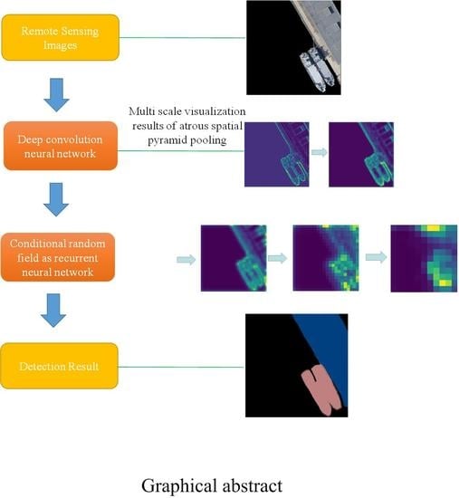
:Under complex sea conditions, ship detection from remote sensing images is easily affected by sea clutter, thin clouds, and islands, resulting in unreliable detection results. In this paper, an end-to-end convolution neural network method is introduced that combines a deep convolution neural network with a fully connected conditional random field. Based on the Resnet architecture, the remote sensing image is roughly segmented using a deep convolution neural network as the input. Using the Gaussian pairwise potential method and mean field approximation theorem, a conditional random field is established as the output of the recurrent neural network, thus achieving end-to-end connection. We compared the proposed method with other state-of-the-art methods on the dataset established by Google Earth and NWPU-RESISC45. Experiments show that the target detection accuracy of the proposed method and the ability of capturing fine details of images are improved. The mean intersection over union is 83.2% compared with other models, which indicates obvious advantages. The proposed method is fast enough to meet the needs for ship detection in remote sensing images.
1. Introduction
With the rapid development of space remote sensing technology, ship detection using remote sensing images research [1] has received considerable attention in the marine field. The world has rich marine resources, and ship detection using remote sensing images is necessary. For example, in the civil field, ports provide special support for the garrison to repair ships. As such, improving the detection, classification, and recognition of ship targets in the port is required. This will strengthen the monitoring and management of the port. When a ship loses contact in poor weather conditions, remote sensing images could be used to quickly and accurately detect the location of the ship in distress, which is conducive to rescue work.
Traditional ship detection methods in remote sensing images include (1) saliency detection [2], which simulates the human visual perception mechanism but detects other significant targets when detecting port ships, such as small islands; (2) edge information detection [3], which is combined with the shape characteristics of the ship and the edge information to obtain the proposal region; (3) detection of the fractal model [4], which completes the automatic detection work according to whether the ship target or other backgrounds have obvious fractal features (however, Methods (3) and (4) have poor detection performance under complex sea conditions); and (4) the semantic segmentation method [5,6], which clusters pixels belonging to the same category in an image into one region. The ship can be clearly separated from the surrounding background. Compared with image classification or target detection, semantic segmentation can describe the image more accurately. The traditional classification methods used for semantic segmentation are (1) random decision forests [7], which is a classification method that uses multiple trees to train and predict samples; (2) Markov random fields [8], which is an undirected graph model that defines markers for each pixel; and (3) condition random field [9,10], which represents a Markov random field with a set of input random variables X and another set of output random variables Y. The test results are affected by real complex nature conditions in remote sensing images, such as thin clouds, ports, and islands. However, the classification effect of these traditional methods is still poor.
Deep learning has been widely used in computer vision, achieving breakthrough success especially in image classification. DeepLab [11,12] was proposed by the Google team for semantics segmentation. Solving the problem of spatial resolution degradation caused by continuous pooling and downsampling in traditional classification deep convolutional neural networks (DCNNs) [13,14] improved the segmentation effect. However, DeepLab still experiences some problems. It uses DCNN for coarse segmentation, then uses the fully connected conditional random field (fully connected CRF) to perform fine segmentation. As such, end-to-end training cannot be achieved, which results in low classification accuracy. In addition, DeepLab’s ability to capture fine details of ship targets is poor.
To solve the above problems, this paper proposes a new semantic segmentation model of convolutional neural networks based on DeepLab, which was applied to ship detection under complex sea conditions. This paper builds further on the work of Chen et al. (References [11] and [12]), with the addition of end-to-end training. Combining CRF with deep convolutional neural networks, and using Gaussian pairwise potential and mean field approximation theorem, the CRF is established as a recurrent neural network (RNN) [15], which is used as part of the neural network [16] to produce a deep end-to-end network with both DCNN and CRF. We call it deep semantic segmentation (DSS). Section 2 reviews the development of semantic segmentation and describes the basic principles of DeepLab. Section 3 is the focus of this paper, and describes the specific method used in ship detection. Section 4 is the experimental section, which verifies the feasibility of the DSS.
2. Related Work
Deep learning [17,18,19] has been widely used in the field of computer vision and has achieved breakthrough success in image classification. Several general architectures have been constructed for deep learning, such as the VGG [20] and Resnet [21] networks. VGG was proposed by the Computer Visual Group of the University of Oxford, which explored the relationship between the depth of the convolutional neural network and its performance. A deep neural network was successfully constructed by repeatedly stacking small convolutional layers and max pooling layers. The advantage is that although the network is deepened, the parameter explosion problem does not occur, and the learning ability is strong. However, more memory is required due to the increase in the number of layers and parameters. Resnet proposed a residual module and introduced an identity map to solve the degradation problem in the depth grid. We assume that the input of a neural network is x and the expected output is H(x). If the input x is directly transmitted to the output as the initial result, the goal we need to learn is F(x) = H(x)-x. This is a Resnet unit, which is equivalent to changing the learning goal and no longer learning a complete output. Compared with VGG, Resnet can deepen the grid as much as possible. Resnet has a lower error rate and low computational complexity.
The segmentation method based on deep learning has developed rapidly. Three semantic segmentation methods are based on deep learning. The first method is based on upsampling. CNN loses some details when sampling. This process is irreversible, leading to low image resolution. Upsampling can fill in some missing information, which results in more accurate segmentation boundaries. For example, Long proposed the fully convolutional networks (FCNs) [22], which are applied to semantic segmentation and are highly accurate. However, FCNs are not sensitive to the details in the image and do not fully consider the relationship between pixels. This produces a lack of spatial consistency. The second method is the probability graph model. For example, the second-order CRF is used to smooth noise and couple adjacent nodes, which is beneficial for assigning similar spatial pixels to the same marker. At this stage of the DCNN, the score map is usually very smooth, and the goal is to restore the detailed local structure. In this case, the traditional conditional random field model will miss small structures. Fully connected CRFs can overcome this shortcoming and capture fine details. The third segmentation method involves improving the feature resolution, restoring the resolution due to the DCNN, and thus obtains more context information. DeepLab [11,12], combined with DCNN and a probability map, can adjust the resolution by atrous convolution, expand the receptive field, and reduce the calculation. The multi-scale feature extraction is performed by atrous spatial pyramid pooling (ASPP) to obtain global and local features. Then, the edge effect is optimized by the fully connected CRF. However, DeepLab cannot achieve end-to-end connectivity.
In the traditional convolution neural network, pooling is usually used to reduce the dimension. This has some side effects on image semantic segmentation. Due to the low pixel size on the feature layer after pooling, the accuracy in the feature map is lost even if upsampling is used. Therefore, the purpose of atrous convolution is to not need a pooling layer. After pooling, pixel information is reduced normally, which leads to information loss. DeepLab uses atrous convolution to enlarge the receptive field. Then, a new feature map operation with a large receptive field is used to achieve more accurate semantic segmentation, which can enlarge the receptive field exponentially without reducing the resolution and size of the feature.
DeepLab uses atrous convolution to sample feature maps, enlarging the receptive field and reducing the steps. Atrous convolution extends the standard convolution operation. By adjusting the receptive field of the convolution filter to capture multi-scale context information, characteristics of different resolutions are output. Considering one-dimensional (1D) signals, the output y of atrous convolution of a 1D input signal x with a filter w(k) of length k is defined in Equation (1) [11,12]. The rate parameter r corresponds to the stride with which we sample the input signal.
DeepLab is based on Resnet and transforms the fully connected layers of Resnet into convolutional layers. The last two pooling layers remove the downsampling and use atrous convolution [11,12] instead of the convolution kernel of the subsequent convolutional layer. Then, DeepLab fine-tunes the weight of Resnet, thereby improving the resolution of the output feature map and enlarging the receptive field. The next step is multi-scale extraction. The traditional method is to input a multi-scale image into the network, and then fuse the features. After trying this method in the network, the network performance improved. However, due to the feature extraction of the input for each scale, the calculation amount increased. Therefore, DeepLab introduces the ASPP operation. By inserting ASPP after the specific convolution layer of the network, the characteristic images of the original image are convoluted using the atrous convolution for different rates. Thus, different scale versions of features can be obtained. This is equivalent to the multi-scale operation of the input image.
DeepLab uses r = (6,12,18,24) 3 × 3 atrous convolution parallel sampling. The results of each atrous convolution branch sampled by ASPP are fused together, and then a final prediction result is obtained. DeepLab scales the image in different degrees through different atrous convolutions, and achieves better results. In ASPP, when the rate is larger, it will be close to the size of the feature map. The 3 × 3 convolution degenerates into a 1 × 1 convolution. So, we changed the rate to (6,12,18). Then, we added the batch normalization (BN) layer in ASPP, which can improve the generalization ability of the network and speed-up the network training.
The contribution of this study is using a deep convolutional neural network to extract object features and achieve an end-to-end connection with fully connected conditional random fields to refine object edges.
3. Ship Detection in Remote Sensing Images under Complex Sea Conditions
Marine remote sensing images are complex and changeable. Islands, thin clouds, sea clutter, and other factors in the images impact target detection. Especially when the ship is located in the port, the results produced by DeepLab are disturbed by the surrounding background, resulting in poor segmentation. This study was based on DeepLab. The input remote sensing image is roughly segmented by DCNN, then the improved fully connected CRF is regarded as RNN, which is used as the output to subdivide the image. The end-to-end connection between DCNN and the fully connected CRF is realized, combining their advantages in a unified end-to-end framework. We improved the atrous convolution rate in the ASPP and added the BN layer to increase the grid training speed. Finally, the fully connected conditional random field algorithm based on the average field approximation theorem was improved, achieving the end-to-end connection with the DCNN.
3.1. Conditional Random Fields
In this section, we provide a brief overview of CRF for pixel-wise labelling. It is a description of the work of Zheng et al. [16]. First, we model a random variable that represents the pixel label; Markov random fields are formed under global observation conditions. Set the picture to I, where xi is the label of pixel i, taking the value from Li. Let X be the vector formed by the random variables x1, x2 … xN, where N is the number of pixels in the image. I and X can be modeled as CRFs [23], as shown in:
The Gibbs distribution is shown in Equation (3).
where is the unary energy components, which measure the cost of the pixel i taking the label xi, obtained here by the DCNN; is the pairwise potential that measures the cost of assigning labels xi,xj to pixels i,j. Depending on image smoothing terms, similar pixels are more likely to label the same label, as shown in Equation (4). fi, fj are the feature vectors of the pixels i and j for two-dimensional (2D) coordinates and color vectors; m represents the number of Gaussian kernels, and takes 1 or 2; each is a Gaussian kernel applied on feature vectors; is the linear combination weight; and the function is the label compatibility function, which acts as a punishment.
3.2. CRF as RNN
According to Equation (3), the labeling result can be obtained by minimizing the Gibbs distribution E(x). This process is complex, and the algorithm is time-consuming. In this paper, we introduce a mean-field approximation to the CRF distribution for approximate maximum posterior marginal inference, where Q(x) is an approximation of P(x), which is reconstructed as an RNN. The mean-field approximation reasoning iterative algorithm [16] is as shown in Table 1.
As shown in Table 1, the first step is initialization. It is equivalent to applying a SoftMax function over the unary potentials U across all the labels at each pixel. This step does not include any parameters, as shown in the SoftMax layer of neural networks. The next step is message passing, i.e., probability transfer; it is realized by applying M Gaussian filters on Q. This is equivalent to the convolution operation of a neural network. The third step is weighting filter outputs. For each class label l, it is taking a weighted sum of the M filter outputs from the previous step. This process can be regarded as a convolutional layer with a 1 × 1 filter, convolution operations on a multiple feature image. The fourth step is compatibility transform. Better results can be obtained by considering compatibility between different tags and allocating penalties accordingly. This can be regarded as another convolution layer where the spatial receptive field of the filter is 1 × 1. If a different label is assigned to a pixel with similar properties, it will be penalized. The fifth step is adding unary potentials, subtracting the output of the fourth step from unary energy. This can convey the error differential. The final probability is determined by the result U and the global probability transfer result . The final step is normalization. The results of the fifth step are normalized to the next iteration of the RNN as the initial probability. This can be seen as another SoftMax operation with no parameters [16,23]. Above is a description of the work of Zheng et al.
In this study, we improved the second and third steps. The original Gaussian kernel considers the location vector and color vector of x,y; that is, the Gaussian kernel is 2. The color vector determines the prior probability of the classification in the DCNN layer, so the Gaussian distance of the color vector can be ignored, and only the location difference needs to be considered. The Gaussian kernel is 1. The farther the distance, the smaller the difference. We propose an improved method by combining the full map distance weight and the network training method. The second and the third step combine the probability transfer and the weight adjustment into a new algorithm, which is equivalent to the convolution operation. As shown in Equation (5), ai is the distance weight, l is the class, and is the class probability for each point.
The process of one iteration is shown in Figure 1, which can be expressed as multiple convolutional neural network layers. We use the function to denote the transformation completed by one mean-field iteration. The multi-layer average-field iteration can repeat the above process implementation, with each iteration obtained from the results of previous iterations. This process is equivalent to an RNN. The network is given by Equations (6)–(8). The initial value of H1(t) is the result of normalization of DCNN, H2(t) is the one-iteration process of CRF, and T is the number of iterations of the average field. When the specified number of iterations T is not reached, the iteration is continued. If t = T, the output H2(t) is the final iteration result.
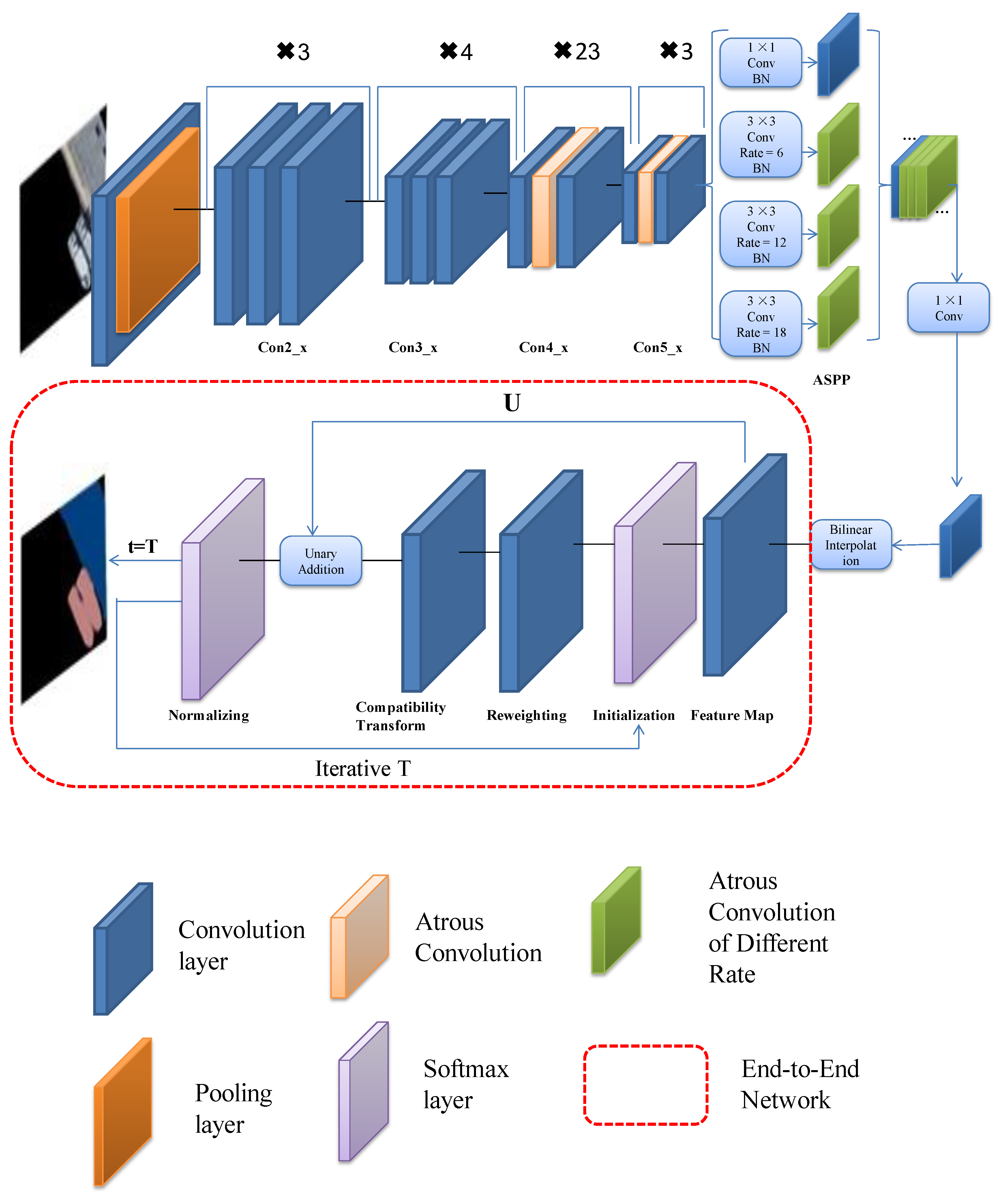
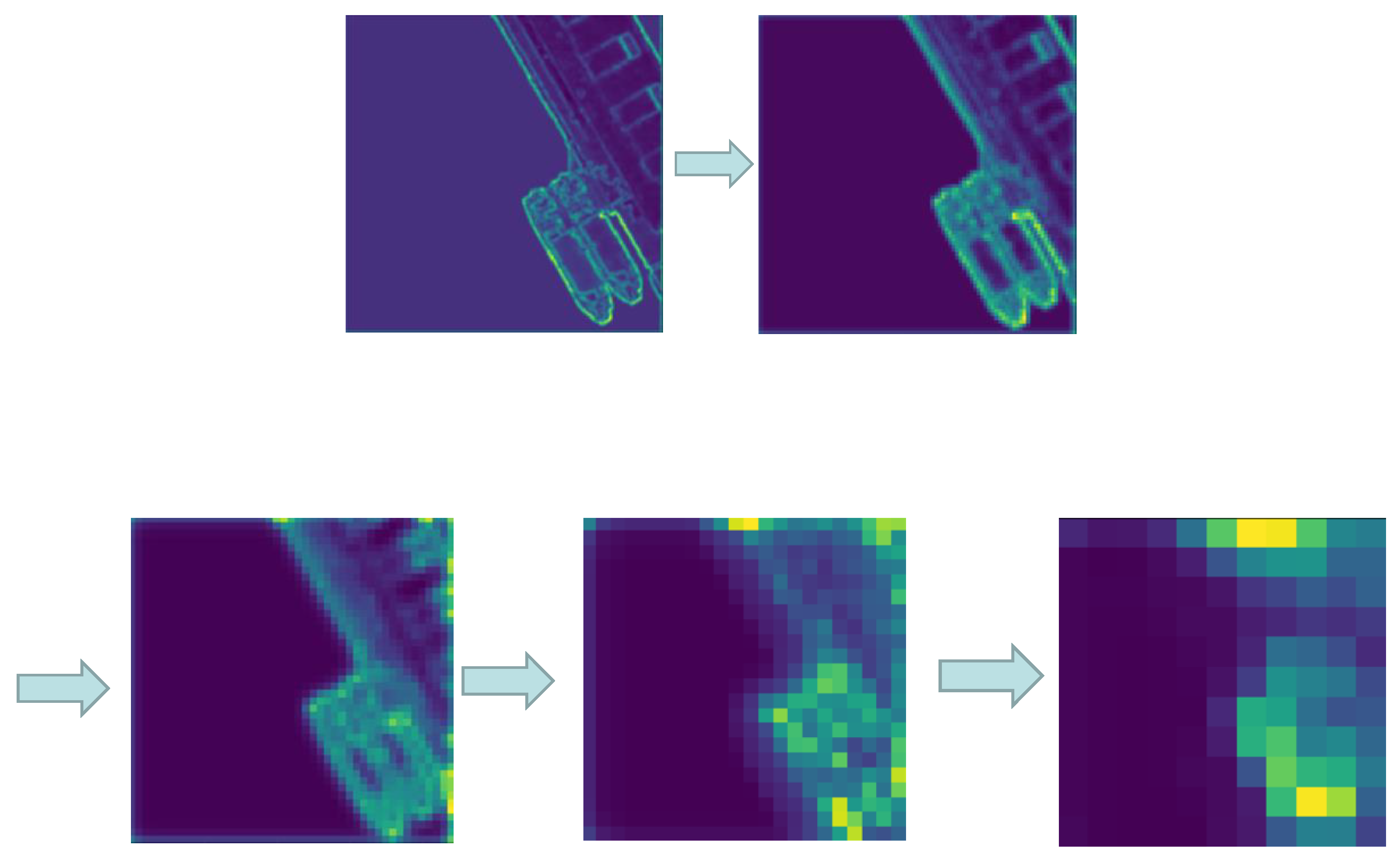
Through the above improvements, the end-to-end algorithm structure is as shown in Figure 2. Firstly, the input image is processed by the Resnet network. We changed the middle layer of Con3_x and Con4_x to atrous convolution. Secondly, the feature maps are obtained by different atrous convolution rates in ASPP. The BN layer increases the training speed and the generalization ability of the network. The convolution neural network visualization of ASPP is shown in Figure 3. When the receptive field is small, the details of the image are extracted. The system extracts the abstract features of the image. Then, it outputs the feature map via bilinear interpolation, which provides the unary potential of CRF. It is connected with the recurrent neural network. Finally, after entering the RNN, the network needs to be iterated t to leave the loop. End-to-end training is performed using the back propagation and stochastic gradient descent algorithms. Once exiting the loop, the SoftMax layer terminates the network. Then, the network outputs the classification results. This algorithm unifies the advantages of DCNN and fully connected CRF, and achieves end-to-end connection.
4. Experiment
In the experiment, our proposed model was used to detect a ship target from a remote sensing image under complex sea conditions and we compared the result with other state-of-the-art methods to verify the advantages of the model. For all experiments, we used the popular Caffe deep learning library. We established a high-quality remote sensing image dataset for ships, which was derived from Google Earth (https://earth.google.com/web/) and NWPU-RESISC45 datasets (http://www.escience.cn/people/JunweiHan/NWPU-RESISC45.html). Google Earth’s satellite images are not a single data source; multiple satellite images are integrated. Part of its satellite images are obtained from the QuickBird commercial satellite and the Earthsat company of the DigitalGlobe company in the United States. The NWPU-RESISC45 dataset is a publicly available benchmark for remote sensing image scene classification (RESISC), created by Northwestern Polytechnical University (NWPU). The total number of the images is 5260. In the experiment, we used the poly strategy in the training process, as shown in Equation (9) [11,12]. The number of iterations in the deep convolution neural network was set to 20,000. An epoch means that all samples in the training set are trained once. We used 80 epochs in these experiments. The initial value of learning rate was 0.001. If the learning rate is too high, it will be unstable when converging to the optimal position. So, the learning rate should decrease exponentially with the training process. We used a weight decay of 0.0005 and momentum of 0.9. The background of the dataset includes a harbor, calm sea, an island, and thin cloud, with 1660 images from offshore ships and 3600 images from nearshore ships. We used 60% of the images to train, 20% to validate, and 20% to test. Finally, we performed data enhancement, which involved rotating each image by 90°, 180°, and 270°. Finally, we obtained a dataset containing 10,520 images. We examined the experimental results including ship semantics segmentation, quantitative analysis, and time analysis.
where power is the parameter and the value is 0.9, iter represents the number of iterations, and max_iter represents the maximum number of iterations.
4.1. Semantic Segmentation Result
Firstly, we compared the results of CRF-RNN (Conditional random field as recurrent neural network), DeepLab, and our method for ship detection. The experimental background was a calm sea, with sea clutter, harbor, thin cloud, and an island.
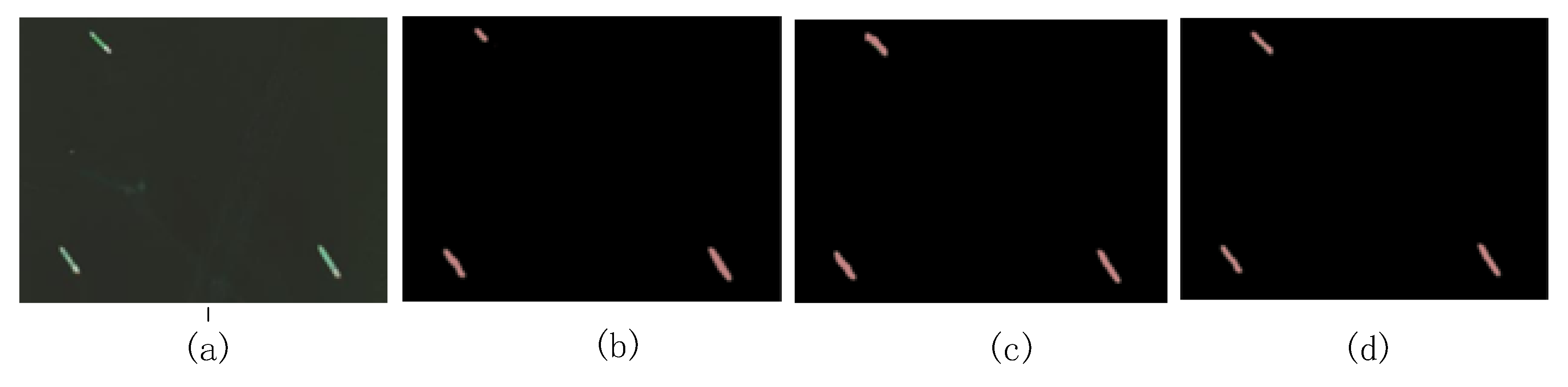
Figure 4 shows the results of ship detection with a calm sea surface. The classification effects of the two models are better than the proposed method, but our method has strong ability to capture the fine details of the target. Figure 5 depicts a calm sea ship with Gaussian noise. The Gaussian noise coefficient was 0.4. From the results of semantic segmentation, CRF-RNN was affected by noise, resulting in missed detection. In the DeepLab result, the edge of ship target is fuzzy. The method proposed in this paper is not affected by noise; it can accurately classify ships. The ship detection results under sea clutter are shown in Figure 6; the CRF-RNN result was the worst. DeepLab captured some details of the image due to the combination of deep learning and a fully connected CRF. However, the edge details are unclear. Our method improves the segmentation accuracy due to the improved end-to-end connection.
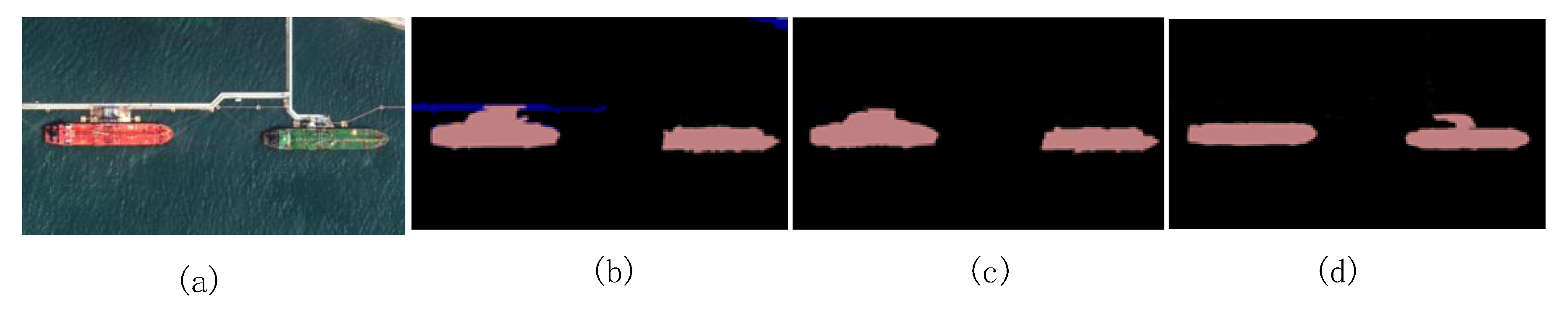
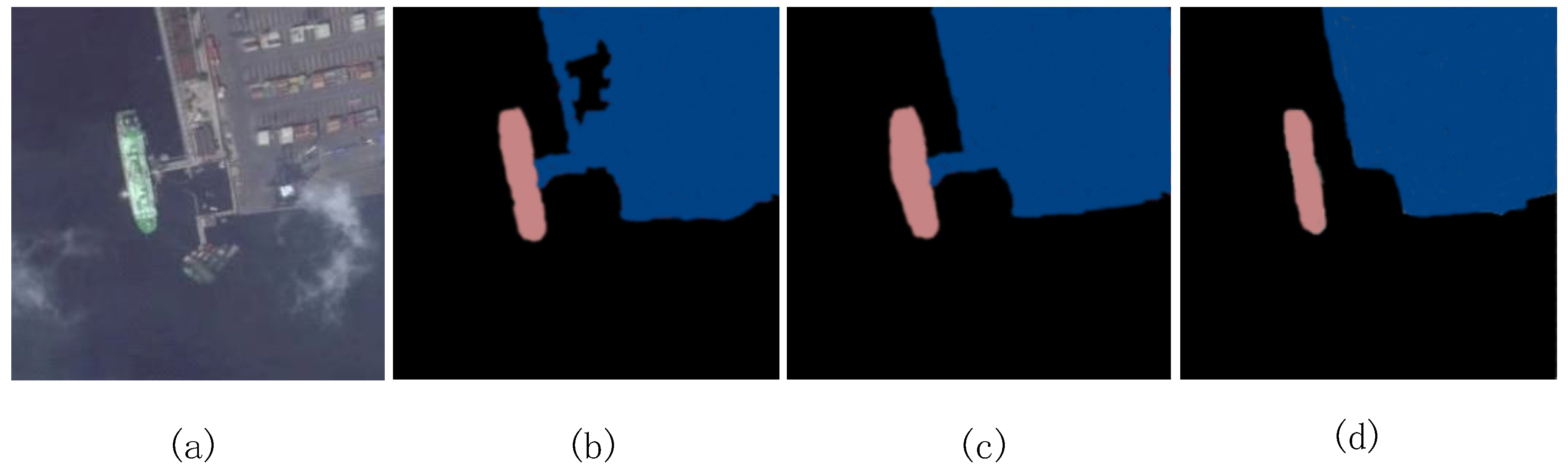
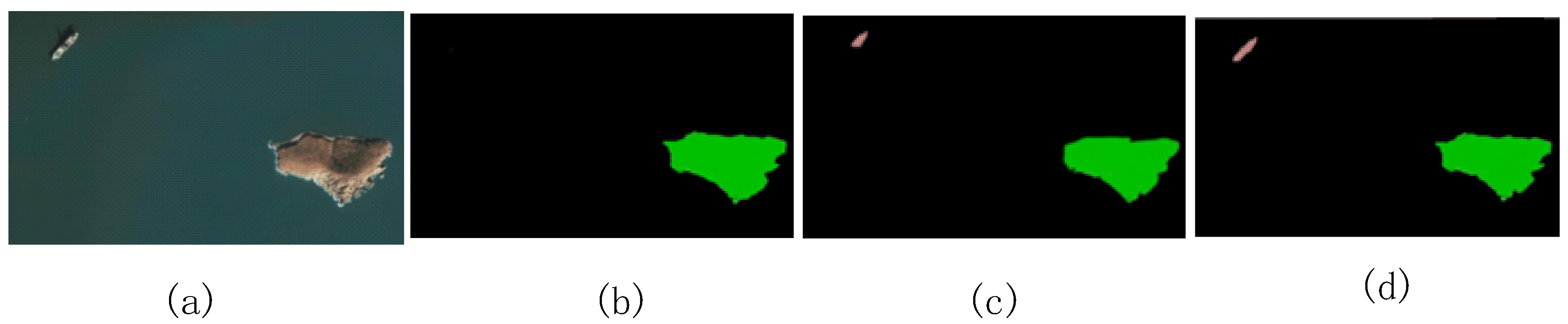
As shown in Figure 7, when the ship was located in the port, the CRF-RNN misclassified one of the ships. Although the DeepLab model correctly classifies the ships and ports, the target edges are already unclear. DSS can overcome their shortcomings and improve the segmentation accuracy. As shown in Figure 8, the background is under the thin cloud The three images all overcome the interference of thin cloud. Our method captures the fine details of the target edge. Figure 9 depicts a semantic segmentation result with the island. The CRF-RNN classifies the ship and the sea surface into one category, resulting in misclassification. DeepLab did not completely classify the objects, but our method correctly classified the islands and ships, and the edge details are clear. The experiments showed that our method is superior to the other models under the conditions of sea clutter, harbor interior, thin clouds, and islands. In addition, the fine details are clearer.
4.2. Quantitative Result
We then quantitatively analyzed the model. Qualitative analysis is not enough, since detailed and specific conclusions cannot be generated. Therefore, quantitative methods can provide more detailed and specific data support for the argumentation process. These methods include precision, recall, F-measure analysis, receiver operating characteristic (ROC) and area under the curve (AUC) analysis, s confusion matrix, and runtime analysis.
4.2.1. Precision, Recall, and F-Measure Analysis
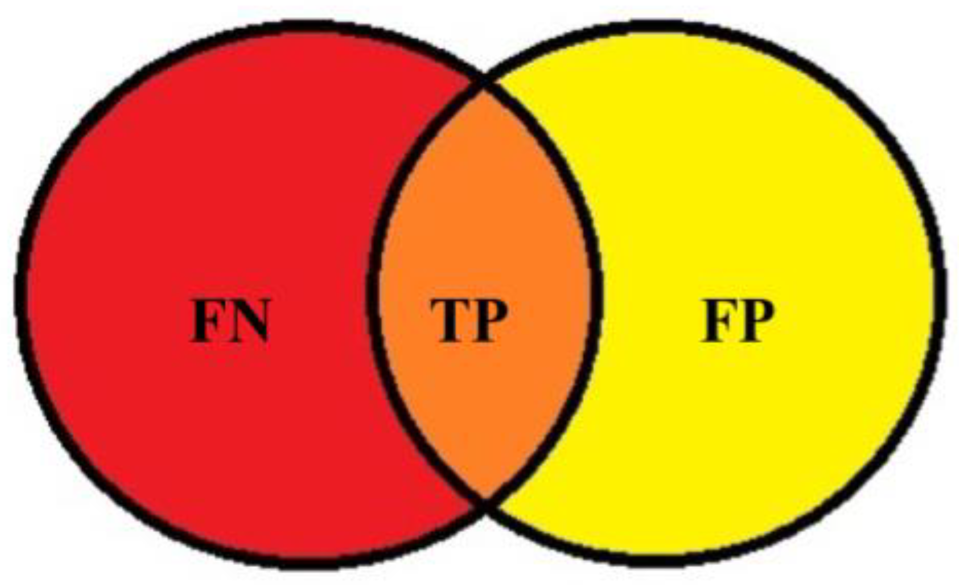
We used precision, recall, and F-measure [24] as evaluation criteria to verify the advantages of the model. Precision is the ratio of the number of positive samples predicted correctly to the number of all predicted positive samples. Recall is the ratio of the number of correctly predicted positive samples to the total number of true positive samples. The F-measure is the weighted harmonic average of precision and recall, which are defined in Equations (10)–(12), respectively.
where TP is true positive, which is a sample that is determined to be positive and is actually positive; FP is false positive, which is a sample determined to be positive, but is actually negative; FN is false negative, which is a sample determined to be negative but is actually positive; and β2 is 1.
Figure 10 shows the quantitative analysis results of the four models. The figure shows that the precision of the proposed model (93.20%) is 6.28% higher than that of DeepLab (86.92%). The recall (79.31%) is 11.24% higher than that of DeepLab (68.07%). The F-measure shows that the model proposed in this paper (85.70%) is better than other models when it comes to ship detection. Because the end-to-end connection is implemented, the accuracy of the model is improved. The F-measures for DeepLab, CRF-RNN, and FCN-8s were 76.35%, 69.42%, and 65.5%, respectively.
4.2.2. ROC and AUC Analysis
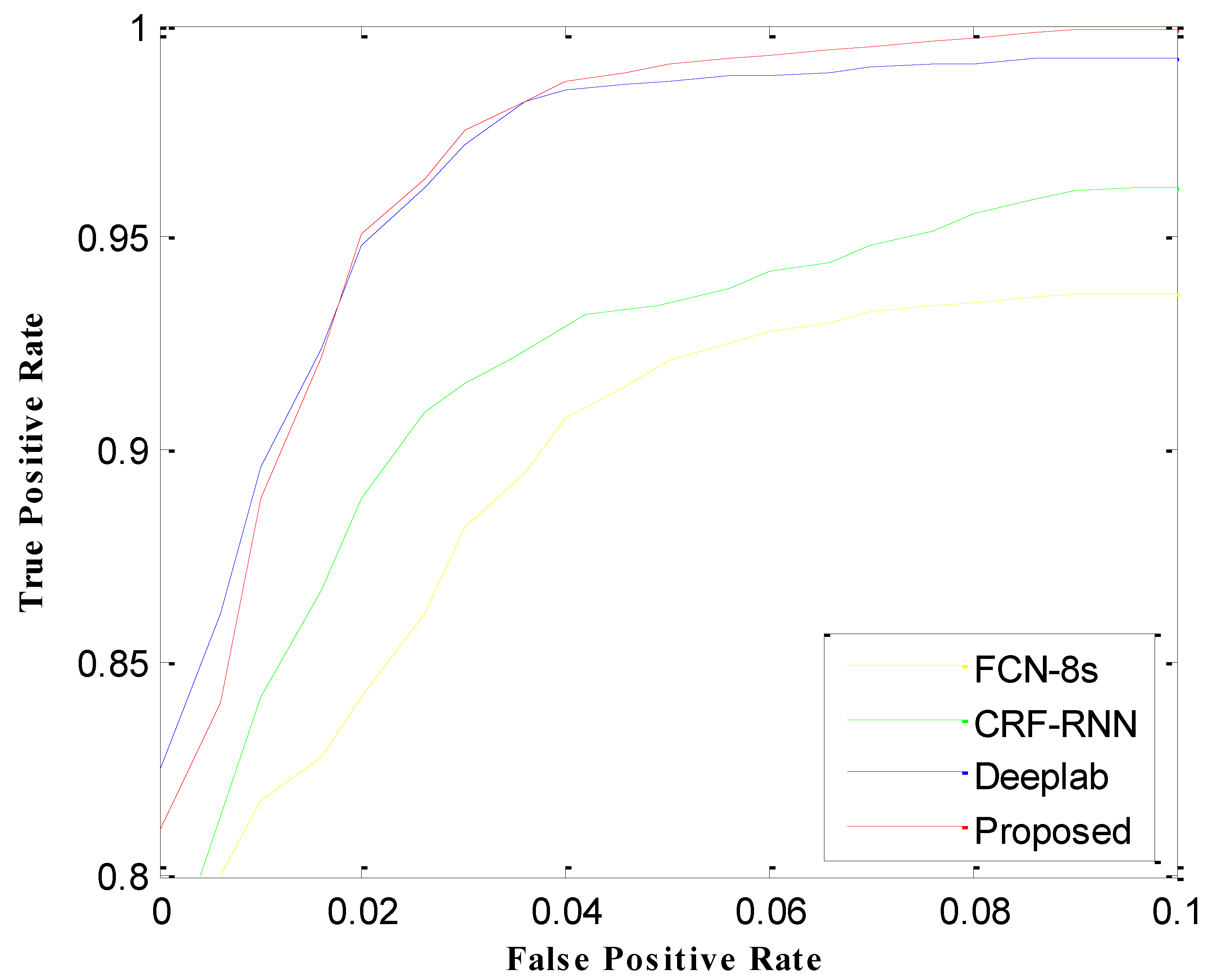
We used the ROC [25] curve to test the performance of the network structure. ROC was originally used to evaluate radar performance. The method is simple and intuitive, and the accuracy of the analysis method can be observed through the diagram. The ROC curve is based on the true positive rate (TPR) as the ordinate, with the false positive rate (FPR) as the abscissa. The ROC curve combines the true positive rate and false positive rate to accurately reflect the performance of the learner. The closer the ROC curve to the top left, the better the performance of the model. The calculation equations are
where TN is true negative, meaning a sample is determined to be a negative and the sample is actually negative.
The experimental results are shown in Figure 11. The models with the worst curve performance were FCN-8s and CRF-RNN. Because the network model is not deep enough, the result was poor. Both DeepLab and the proposed model are better, with the curves being close to the top left. However, our method is better than DeepLab because it realizes the end-to-end connection between the deep convolution neural network and the fully connected conditional random field, so the effect is better.
The area under the curve (AUC) [26] is defined as the area enclosed by the coordinate axis under the ROC curve. The value of this area cannot be greater than 1. Because the ROC curve is generally above the line y = x, the value of AUC ranges between 0.5 and 1. The closer the AUC is to 1.0, the higher the accuracy of the detection method. When the AUC value is equal to 0.5, the accuracy is the lowest, so the method has no application value. The AUC values of our model and the other advanced methods are shown in Table 2, which shows that the AUC value of our method is the highest, meaning it has the best performance.
4.2.3. Confusion Matrix
To verify the accuracy of the proposed algorithm, an experimentally measured classification confusion matrix [27,28,29,30] for ship target recognition was used. This matrix is primarily used for evaluating the classification accuracy of an image. Each column represents a prediction category, and the total number of data in each column represents the percentage of data projected for that category. Each row represents the true category of data, and the total number of data in each row is the percentage of table instances. For example, the value in the first column of the first row indicates the probability of a ship actually belonging to the first category being predicted as the first category. The value of the first row and the second column indicates the probability of a ship actually belonging to the first category being mispredicted as the second category. The other values are calculated in the same way. The confusion matrix of this algorithm is shown in Table 3.
Table 3 shows that the classification accuracy for the port was the lowest. This occurred due to the complex background provided by the port. The methods are most likely to judge incorrectly here between ships and ports. Ships that sometimes dock in the port, connecting to the port, lead to classification errors. The classification accuracy of the proposed method is high, thereby satisfying the needs for remote sensing image ship target recognition.
4.2.4. Runtime Analysis
Table 4 compares the runtime of the proposed method with those of other state-of-the-art models. The table shows that DeepLab takes up to 1 s because the end-to-end connection between the DCNN and fully connected CRF is not realized. DSS is relatively fast and DSS and FCN-8s are in the same order of magnitude, guaranteeing the detection accuracy.
5. Discussion
In this section, to better discuss these results and analyze how they can be interpreted with respect to other studies, we compared the mIOU value with state-of-the-art models.
5.1. mIOU Analysis
We compared our method with the state-of-the-art models on the established dataset, as shown in Table 5. The performance was measured in terms of pixel mean-intersection-over-union (mIOU) [31]. The mIOU results are depicted in Figure 12. mIOU calculates the ratio between the intersection of two circles and the union of two circles, and is the standard measure of semantic segmentation, as shown in Equation (15). Divmbest had the lowest mIOU value of 49.5, CRF-RNN was 73.1, and DeepLab ranked second, at 78.3. When it comes to ship detection, the proposed method was better than other state-of-the-art models, with an mIOU of 83.2.
where k is the category, i is the true value, j is the predicted value, and pij is predicting class i as class j.
In this study, we compared the effects of the BN layer, ASPP, atrous convolution, and CRF on the dataset established in this paper. The results are shown in Table 6. Adding a BN layer had little effect on the accuracy of segmentation results because the BN layer is mainly used to speed up network training and reduce time consumption. When atrous convolution is used instead of the traditional convolution operation, the result significantly improved because the atrous convolution operation expands the receptive field and improves the output feature map resolution. The mIOU of the method without using the CRF was 81.4. The CRF can refine the edge of the picture and increase the accuracy. Using the improved mean field theorem and the end-to-end connection method, the segmentation accuracy is improved. To summarize, the method proposed in this paper produces significantly improved segmentation results.
We compared the effect of the CRF iterations on the experimental results; the results are reported in Table 7, which shows that when the number of iterations reached five or more, the mIOU did not significantly improve. Consider the time taken by the iteration, we used T = 5 in this paper.
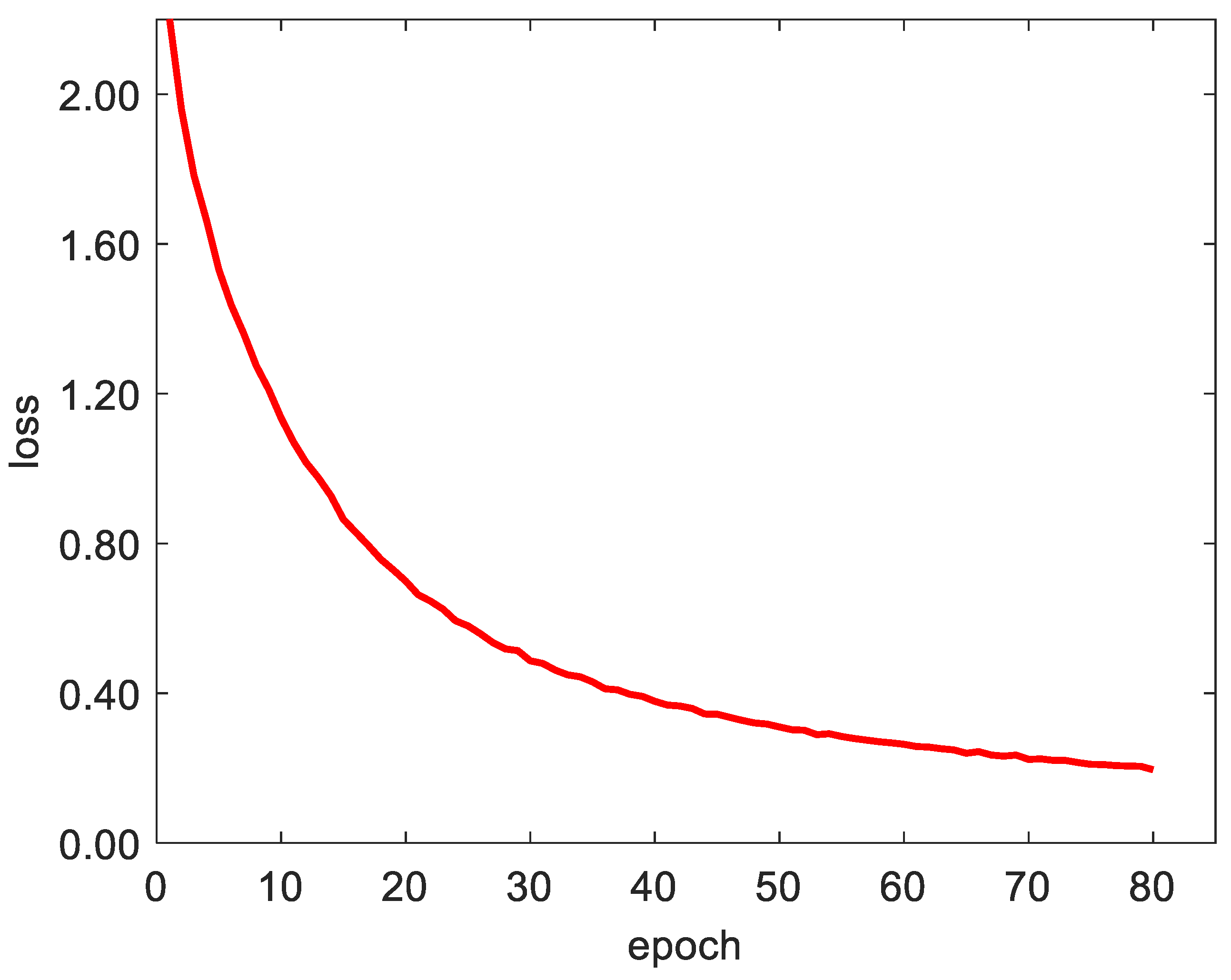
We used the cross-entropy cost [36] function to calculate the loss. Its definition is shown in Equation (16). Cross entropy represents the difference between the true probability distribution and the predicted probability distribution. In deep learning, the true distribution has been determined. The smaller the cross entropy, the better the prediction effect. The loss function curve is shown in Figure 13.
where p(xi) represents the true probability distribution and q(xi) represents the predicted probability distribution.
5.2. Comprehensive Analysis
Traditional methods will miss the targets or detect other objects when detecting the ship. So, we introduced a deep learning method that learns the target characteristics using a deep convolution neural network. Our proposed method produced good results and includes many methods of deep learning. In summary, our method is superior to other models per the qualitative, quantitative, and mIOU analyses. It meets the requirements of ship detection under complex sea conditions, such as sea clutter, thin clouds, ports, and islands. Compared with other state-of-the-art models, our method has obvious advantages.
6. Conclusions
DeepLab is based on DCNN, where atrous convolution replaces the max pooling layer and multi-scale is added, but an end-to-end connection is not achieved with the fully connected CRF. In this study, we considered the fully connected CRF as the RNN and constructed a deep network with both DCNN and CRF characteristics. The end-to-end connection was realized, overcoming the problem of ambiguous edges in ship detection and improving the ability to capture fine details of ship targets. The proposed method is superior to other models under conditions including sea clutter, harbor interiors, thin clouds, and islands. On the established Google Earth and NWPU-RESISC45 dataset, the mIOU of the method is 83.2. The focus of future research will be on how to improve the accuracy of segmentation while maintaining segmentation speed.
Author Contributions
Conceptualization, Y.C. and Y.L.; software, Y.L., X.Z., W.C.; writing—original draft preparation, Y.L., Y.C.; writing—review and editing, Y.C. and J.W. supervision, Y.C. and J.W. funding acquisition, Y.C. All authors have read and agreed to the published version of the manuscript.
Funding
This research was funded by Chinese National Natural Science Foundation (no. 61901081) and the Fundamental Research Funds for the Central Universities (no. 3132018180).
Conflicts of Interest
The authors declare that they have no conflicts of interest.
References
- Cheng, G.; Han, J. A survey on target detection in optical remote sensing images. ISPRS J. Photogramm. Remote Sens. 2016, 117, 11–28. [Google Scholar] [CrossRef] [Green Version]
- Zhang, J.; Sclaroff, S. Saliency detection: A boolean map approach. In Proceedings of the IEEE International Conference on Computer Vision, Sydney, Australia, 1–8 December 2013; pp. 153–160. [Google Scholar]
- Shi, Z.; Yu, X.; Jiang, Z.; Li, B. Ship detection in high-resolution optical imagery based on anomaly detector and local shape feature. IEEE Trans. Geosci. Remote Sens. 2014, 52, 4511–4523. [Google Scholar]
- Liu, N.B.; Ding, H.; Tian, Y.H.; Wen, A.L.; Guan, J. Target detection method in sea clutter based on combined fractal characyeristics. Aero Weapon. 2018, 2018, 38–42. [Google Scholar]
- Noh, H.; Hong, S.; Han, B. Learning deconvolution network for semantic segmentation. In Proceedings of the IEEE International Conference on Computer Vision, Santiago, Chile, 7–15 December 2015; pp. 1520–1528. [Google Scholar]
- Chen, L.C.; Zhu, Y.; Papandreou, G.; Schroff, F.; Adam, H. Encoder-decoder with atrous separable convolution for semantic image segmentation. In Proceedings of the European Conference on Computer Vision (ECCV), Munich, Germany, 8–14 September 2018; pp. 801–818. [Google Scholar]
- Shotton, J.; Johnson, M.; Cipolla, R. Semantic texton forests forimage categorization and segmentation. In Proceedings of the 2008 IEEE Conference on Computer Vision and Pattern Recognition, Anchorage, AK, USA, 23–28 June 2008. [Google Scholar]
- Ranalli, M.; Lagona, F.; Picone, M.; Zambianchi, E. Segmentation of sea current fields by cylindrical hidden Markov models: a composite likelihood approach. J. R. Stat. Soc. Ser. C (Appl. Stat.) 2018, 67, 575–598. [Google Scholar] [CrossRef]
- Varma, K.I.; Krishnamoorthy, S.; Pisipati, R.K. Natural Language Querying with Cascaded Conditional Random Fields. U.S. Patent 9,280,535, 8 March 2016. [Google Scholar]
- Zhao, J.; Zhong, Y.; Shu, H.; Zhang, L. High-resolution image classification integrating spectral-spatial-location cues by conditional random fields. IEEE Trans. Image Process. 2016, 25, 4033–4045. [Google Scholar] [CrossRef]
- Chen, L.C.; Papandreou, G.; Kokkinos, I.; Murphy, K.; Yuille, A.L. Deeplab: Semantic image segmentation with deep convolutional nets, atrous convolution, and fully connected crfs. IEEE Trans. Pattern Anal. Mach. Intell. 2017, 40, 834–848. [Google Scholar] [CrossRef]
- Chen, L.C.; Papandreou, G.; Kokkinos, I.; Murphy, K.; Yuille, A.L. Semantic image segmentation with deep convolutional nets and fully connected crfs. arXiv 2014, arXiv:1412.7062. [Google Scholar]
- Krizhevsky, A.; Sutskever, I.; Hinton, G.E. Imagenet classification with deep convolutional neural networks. In Advances in Neural Information Processing System; Neural Information Processing Systems Foundation, Inc. (NIPS): Lake Tahce, NV, USA, 2012; pp. 1097–1105. [Google Scholar] [CrossRef]
- Sainath, T.N.; Mohamed, A.R.; Kingsbury, B.; Ramabhadran, B. Deep convolutional neural networks for LVCSR. In Proceedings of the 2013 International Conference on Acoustics, Speech and Signal Processing, Vancouver, BC, Canada, 26–31 May 2013; IEEE: Vancouver, BC, Canada; pp. 8614–8618. [Google Scholar]
- Graves, A.; Mohamed, A.; Hinton, G. Speech recognition with deep recurrent neural networks. In Proceedings of the 2013 IEEE International Conference on Acoustics, Speech and Signal Processing, Vancouver, BC, Canada, 1–8 December 2013; IEEE: Vancouver, BC, Canada; pp. 6645–6649. [Google Scholar]
- Zheng, S.; Jayasumana, S.; Romera-Paredes, B.; Vineet, V.; Su, Z.; Du, D.; Huang, C.; Torr, P.H. Conditional random fields as recurrent neural networks. In Proceedings of the IEEE International Conference on Computer Vision, Santiago, Chile, 7–15 December 2015; pp. 1529–1537. [Google Scholar]
- Akhtar, N.; Mian, A. Threat of adversarial attacks on deep learning in computer vision: A survey. IEEE Access 2018, 6, 14410–14430. [Google Scholar] [CrossRef]
- LeCun, Y.; Bengio, Y.; Hinton, G. Deep learning. Nature 2015, 521, 436. [Google Scholar] [CrossRef]
- Schmidhuber, J. Deep learning in neural networks: An overview. Neural Netw. 2015, 61, 85–117. [Google Scholar] [CrossRef] [PubMed] [Green Version]
- Karen Simonyan, A.Z. Very Deep Convolutional Networks for Large-Scale Image Recognition. arXiv 2015, arXiv:1409.1556. [Google Scholar]
- He, K.; Zhang, X.; Ren, S.; Sun, J. Deep Residual Learning for Image Recognition. In Proceedings of the IEEE Conference on Computer Vision and Pattern (In CVPR), Boston, MA, USA, 8–11 June 2015; pp. 770–778. [Google Scholar]
- Long, J.; Shelhamer, E.; Darrell, T. Fully convolutional networks for semantic segmentation. In Proceedings of the IEEE Conference on Computer Vision and Pattern Recognition, Boston, MA, USA, 8–11 June 2015; pp. 3431–3440. [Google Scholar]
- Krähenbühl, P.; Koltun, V. Efficient inference in fully connected crfs with gaussian edge potentials. In Proceedings of the NIPS, Sierra Nevada, Spain, 12–14 December 2011. [Google Scholar]
- Powers, D.M. Evaluation: from precision, recall and F-measure to ROC, informedness, markedness and correlation. J. Mach. Learn. Technol. 2011, 2011, 37–63. [Google Scholar]
- Fan, J.; Upadhye, S.; Worster, A. Understanding receiver operating characteristics (ROC) curves. Can. J. Emerg. Med. 2006, 8, 19–20. [Google Scholar] [CrossRef] [PubMed]
- Lobo, J.M.; Jiménez-Valverde, A.; Real, R. AUC: a misleading measure of the performance of predictive distribution models. Glob. Ecol. Biogeogr. 2008, 17, 145–151. [Google Scholar] [CrossRef]
- Ting, K.M. Confusion matrix. Encycl. Mach. Learn. Data Min. 2017, 2017, 260. [Google Scholar]
- Deng, X.; Liu, Q.; Deng, Y.; Mahadevan, S. An improved method to construct basic probability assignment based on the confusion matrix for classification problem. Inf. Sci. 2016, 340, 250–261. [Google Scholar] [CrossRef]
- Ohsaki, M.; Wang, P.; Matsuda, K.; Katagiri, S.; Watanabe, H.; Ralescu, A. Confusion-matrix-based kernel logistic regression for imbalanced data classification. IEEE Trans. Knowl. Data Eng. 2017, 29, 1806–1819. [Google Scholar] [CrossRef]
- Berman, M.; Rannen Triki, A.; Blaschko, M.B. The Lovász-Softmax loss: A tractable surrogate for the optimization of the intersection-over-union measure in neural networks. In Proceedings of the IEEE Conference on Computer Vision and Pattern Recognition, Boston, MA, USA, 18–22 June 2018; pp. 4413–4421. [Google Scholar]
- Lin, G.; Shen, C.; Reid, I.; van dan Hengel, A. Efficient piecewise of deep structured models for semantic segmentation. arXiv 2015, arXiv:1504.01013. [Google Scholar]
- Payman Yadollahpour, D.B. Discriminative re-ranking of diverse segmentations. In Proceedings of the CVPR, Boston, MA, USA, 18–22 June 2018. [Google Scholar]
- Hariharan, B.; Arbeláez, P.; Girshick, R.; Malik, J. Simultaneous detection and segmentation. In Proceedings of the ECCV, Zurich, Switzerland, 6–12 September 2014. [Google Scholar]
- Yan, Z.; Zhang, H.; Jia, Y.; Breuel, T.; Yu, Y. Combining the best of convolutional layers and recurrent layers: A hybrid network for semantic segmentation. arXiv 2016, arXiv:1603.04871. [Google Scholar]
- Arnab, A.; Jayasumana, S.; Zheng, S.; Torr, P. Higher order potentials in end-to-end trainable conditional random fields. arXiv 2015, arXiv:1511.08119. [Google Scholar]
- Kline, D.M.; Berardi, V.L. Revisiting squared-error and cross-entropy functions for training neural network classifiers. Neural Comput. Appl. 2005, 14, 310–318. [Google Scholar] [CrossRef]
Figure 1.
The mean-field approximation reasoning algorithm iterative process.
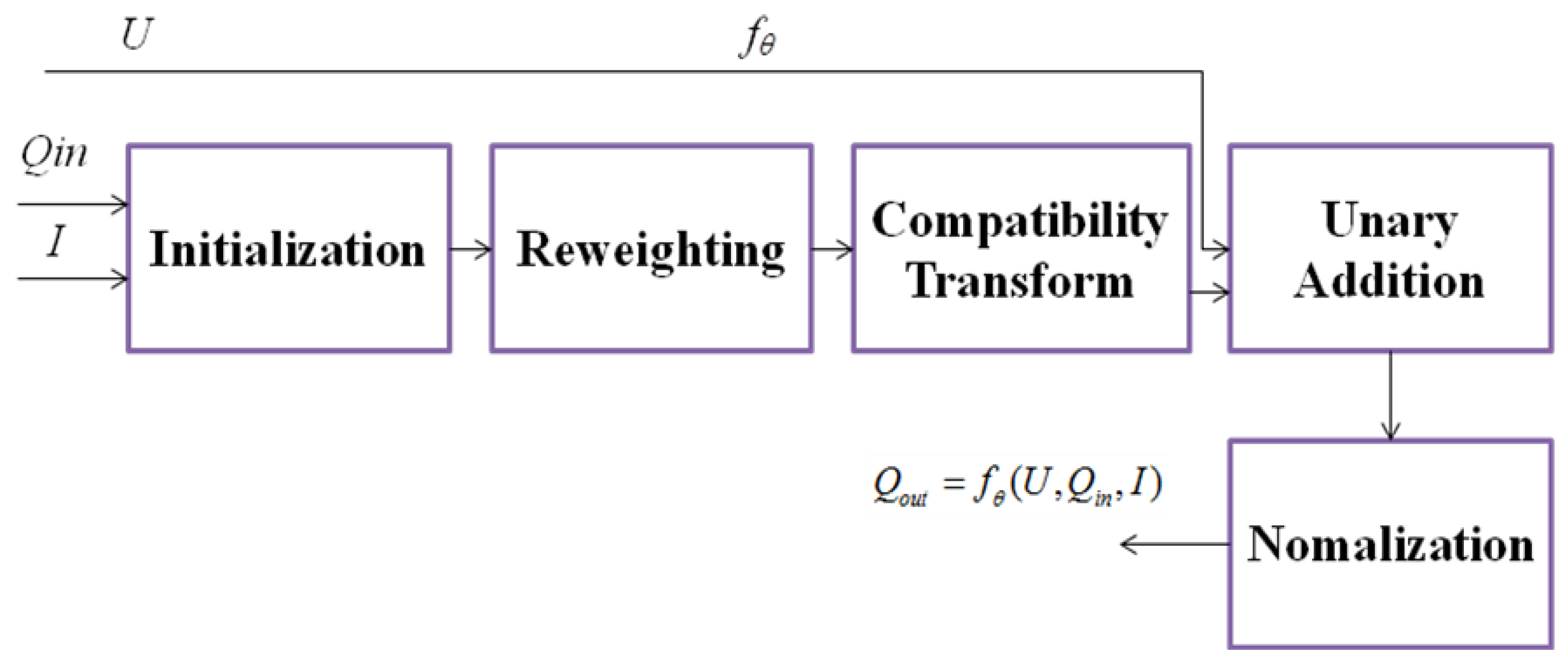
Figure 2.
Deep semantic segmentation (DSS) convolution structure diagram.

Figure 3.
Multi scale visualization results of atrous spatial pyramid pooling (ASPP).

Figure 4.
Semantic segmentation of ships under a calm sea surface. (a) Original (b) Conditional random field as recurrent neural network (CRF-RNN) (c) DeepLab (d) Proposed model.
Figure 4.
Semantic segmentation of ships under a calm sea surface. (a) Original (b) Conditional random field as recurrent neural network (CRF-RNN) (c) DeepLab (d) Proposed model.

Figure 5.
Semantic segmentation of ships under a calm sea surface with Gaussian noise.(a) Original (b)CRF-RNN (c) DeepLab (d) Proposed model.
Figure 5.
Semantic segmentation of ships under a calm sea surface with Gaussian noise.(a) Original (b)CRF-RNN (c) DeepLab (d) Proposed model.
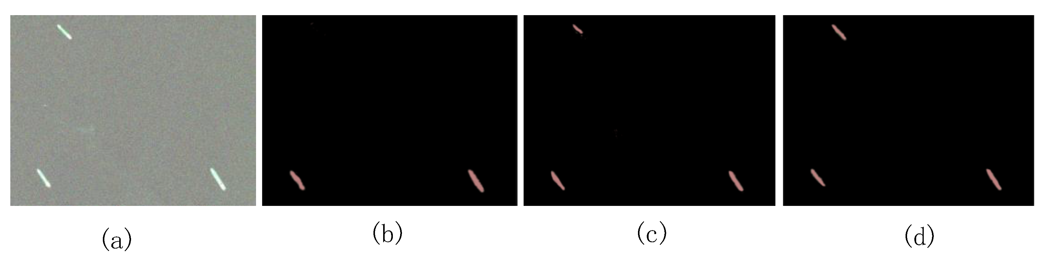
Figure 6.
Semantic segmentation of ships under sea clutter. (a) Original (b)CRF-RNN (c) DeepLab (d) Proposed model.
Figure 6.
Semantic segmentation of ships under sea clutter. (a) Original (b)CRF-RNN (c) DeepLab (d) Proposed model.

Figure 7.
Semantic segmentation of ships within a port. (a) Original (b)CRF-RNN (c) DeepLab (d) Proposed model.
Figure 7.
Semantic segmentation of ships within a port. (a) Original (b)CRF-RNN (c) DeepLab (d) Proposed model.
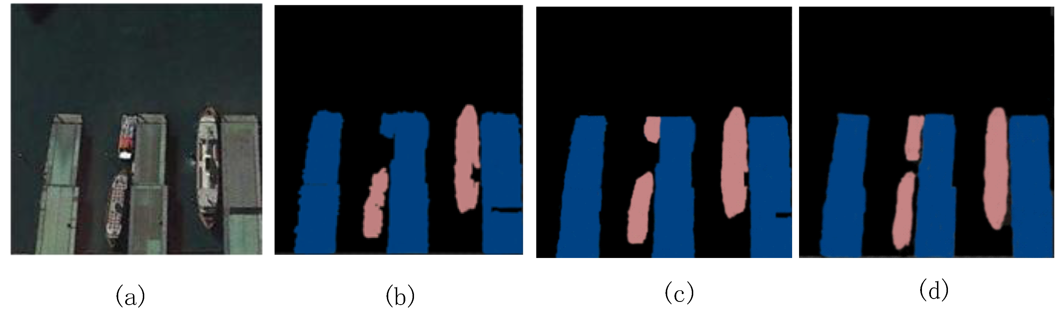
Figure 8.
Semantic segmentation of ships under thin clouds. (a) Original (b)CRF-RNN (c) DeepLab (d) Proposed model.
Figure 8.
Semantic segmentation of ships under thin clouds. (a) Original (b)CRF-RNN (c) DeepLab (d) Proposed model.

Figure 9.
Semantic segmentation of ships with an island(a) Original (b)CRF-RNN (c) DeepLab (d) Proposed model.
Figure 9.
Semantic segmentation of ships with an island(a) Original (b)CRF-RNN (c) DeepLab (d) Proposed model.

Figure 10.
The precision, recall, and F-measure results of the four models.
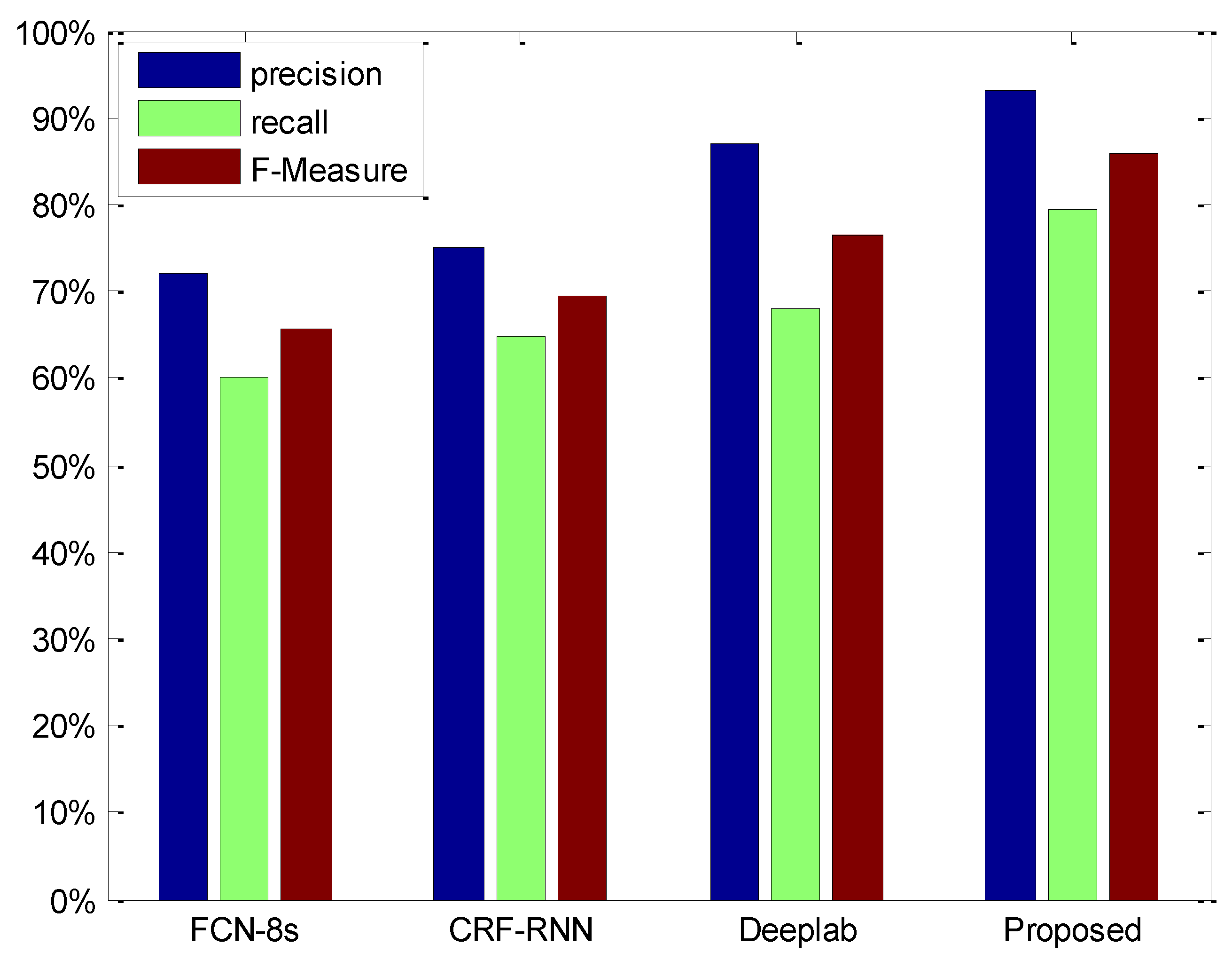
Figure 11.
Receiver operating characteristic (ROC) curve analysis of the four methods.

Figure 12.
Depiction of the mean-intersection-over-union (mIOU).

Figure 13.
Loss function curve.

Table 1.
Mean-field approximation reasoning iterative algorithm.
| Algorithm 1. Mean field in dense CRFs, broken down to common DCNN operations. | |
| Initialization | |
| While not converged do | |
| Message Passing | |
| Weighting Filter Outputs | |
| Compatibility Transform | |
| Adding Unary Potentials | |
| Normalizing | |
| end while | |
Table 2.
Area under the curve (AUC) values of different models.
| Method | AUC |
|---|---|
| FCN-8s | 0.65 |
| CRF-RNN [16] | 0.73 |
| DeepLab [12] | 0.87 |
| Proposed | 0.92 |
Table 3.
Confusion matrix of ship classification.
| Ship | Island | Port | Background | |
| Ship | 0.94 | 0.00 | 0.04 | 0.02 |
| Island | 0.00 | 0.98 | 0.00 | 0.00 |
| Port | 0.05 | 0.00 | 0.93 | 0.00 |
| Background | 0.00 | 0.02 | 0.00 | 0.95 |
Table 4.
Runtime analysis of different models.
| Method | Runtime (s) |
|---|---|
| FCN-8s | 0.5 |
| DeepLab | 1 |
| DeepLab-MSc | 1.2 |
| DSS | 0.75 |
Table 5.
Mean IOU accuracy of our approach and other state-of-the-art approaches.
| Method | mIOU |
|---|---|
| FCN-8s [31] | 62.2 |
| DeepLab-MSc [12] | 71.6 |
| CRF-RNN [16] | 73.1 |
| DeepLab [12] | 78.3 |
| Divmbest [32] | 49.5 |
| SDS [33] | 51.6 |
| H-ReNet+DenseCRF [34] | 76.8 |
| OxfordTVG HO CRF [35] | 77.9 |
| Proposed | 83.2 |
Table 6.
Employing the model on the dataset.
| BN | ASPP | DSS without CRF | Atrous Convolution | CRF | End-to-End Connection with Improved CRF | mIOU |
|---|---|---|---|---|---|---|
| ✓ | ✓ | 76.9 | ||||
| ✓ | ✓ | ✓ | 80.2 | |||
| ✓ | ✓ | ✓ | ✓ | 81.4 | ||
| ✓ | ✓ | ✓ | 82.9 | |||
| ✓ | ✓ | ✓ | ✓ | 82.7 | ||
| ✓ | ✓ | ✓ | ✓ | 83.2 |
Table 7.
Effect of the CRF iterations.
| Iteration | 1 | 2 | 3 | 4 | 5 | 6 | 7 | 8 | 9 | 10 |
| mIOU | 81.6 | 82 | 82.5 | 82.9 | 83.2 | 83.3 | 83.4 | 83.5 | 83.6 | 83.7 |
© 2020 by the authors. Licensee MDPI, Basel, Switzerland. This article is an open access article distributed under the terms and conditions of the Creative Commons Attribution (CC BY) license (http://creativecommons.org/licenses/by/4.0/).
Share and Cite
MDPI and ACS Style
Chen, Y.; Li, Y.; Wang, J.; Chen, W.; Zhang, X. Remote Sensing Image Ship Detection under Complex Sea Conditions Based on Deep Semantic Segmentation. Remote Sens. 2020, 12, 625. https://0-doi-org.brum.beds.ac.uk/10.3390/rs12040625
AMA Style
Chen Y, Li Y, Wang J, Chen W, Zhang X. Remote Sensing Image Ship Detection under Complex Sea Conditions Based on Deep Semantic Segmentation. Remote Sensing. 2020; 12(4):625. https://0-doi-org.brum.beds.ac.uk/10.3390/rs12040625
Chicago/Turabian StyleChen, Yantong, Yuyang Li, Junsheng Wang, Weinan Chen, and Xianzhong Zhang. 2020. "Remote Sensing Image Ship Detection under Complex Sea Conditions Based on Deep Semantic Segmentation" Remote Sensing 12, no. 4: 625. https://0-doi-org.brum.beds.ac.uk/10.3390/rs12040625
Note that from the first issue of 2016, this journal uses article numbers instead of page numbers. See further details here.