The Determination of Aerosol Distribution by a No-Blind-Zone Scanning Lidar

Abstract

A homemade portable no-blind zone laser detection and ranging (lidar) system was designed to map the three-dimensional (3D) distribution of aerosols based on a dual-field-of-view (FOV) receiver system. This innovative lidar prototype has a space resolution of 7.5 m and a time resolution of 30 s. A blind zone of zero meters, and a transition zone of approximately 60 m were realized with careful optical alignments, and were rather meaningful to the lower atmosphere observation. With a scanning platform, the lidar system was used to locate the industrial pollution sources at ground level. The primary parameters of the transmitter, receivers, and detectors are described in this paper. Acquiring a whole return signal of this lidar system represents the key step to the retrieval of aerosol distribution with applying a linear joining method to the two FOV signals. The vertical profiles of aerosols were retrieved by the traditional Fernald method and verified by real-time observations. To effectively and reliably retrieve the horizontal distributions of aerosols, a composition of the Fernald method and the slope method were applied. In this way, a priori assumptions of even atmospheric conditions and the already-known reference point in the lidar equation were avoided. No-blind-zone vertical in-situ observation of aerosol illustrated a detailed evolution from almost 0 m to higher altitudes. No-blind-zone detection provided tiny structures of pollution distribution in lower atmosphere, which is closely related to human health. Horizontal field scanning experiments were also conducted in the Shandong Province. The results showed a high accuracy of aerosol mass movement by this lidar system. An effective quantitative way to locate pollution sources distribution was paved with the portable lidar system after validation by the mass concentration of suspended particulate matter from a ground air quality station.

1. Introduction

The gradient of energy distribution affects the evolution of the atmospheric boundary layer (ABL), and mainly induces the uneven distribution of aerosol and the formation and deterioration of air quality [1,2,3,4,5]. The transport of dust storms and smoke has caused severe regional air pollution on several occasions [6,7,8]. Laser detection and ranging (lidar), as an active remote-sensing technique, is often utilized to detect and identify the physical properties, shapes and particle-size distribution of aerosols with a high spatial and temporal resolution from ground stationary lidar networks [9,10], mobile platforms [11], aircrafts [12] or satellites [13]. However, due to a monostatic receiving field and “geometric overlap factor (GOF)”, the hundreds of meters of blind zone and the transition zone in traditional Mie-lidars [14,15,16,17,18,19,20] always lead to a difficulty in probing aerosols, especially in the lower troposphere [21,22,23]. A few groups have developed side-scattering imaging technologies [24,25,26,27] or multi-field-of-view (mFOV) techniques [28,29] to overcome such difficulties. However, the former methods are limited as the detection range ignores important information from the distant atmosphere, and the latter methods are laboratory instruments that are difficult to move. In this study, a compact portable dual-field-of-view (FOV) lidar prototype aimed at narrowing the transition zone is demonstrated. A reliable inversion method for determining the vertical and horizontal distributions of aerosols within 5 km is provided. Field experiments were also conducted to verify the applicability of the dual-FOV lidar for studying lower-atmosphere air pollution and quantitatively assessing the distribution of emission sources. With this scanning lidar, the pollution distribution near ground can be identified with no-blind-zone and quantitatively. The established lidar network with this kind of lidars can be used to study the pollution transport pathways.

2. Materials and Methods

2.1. Dual-FOV Lidar System

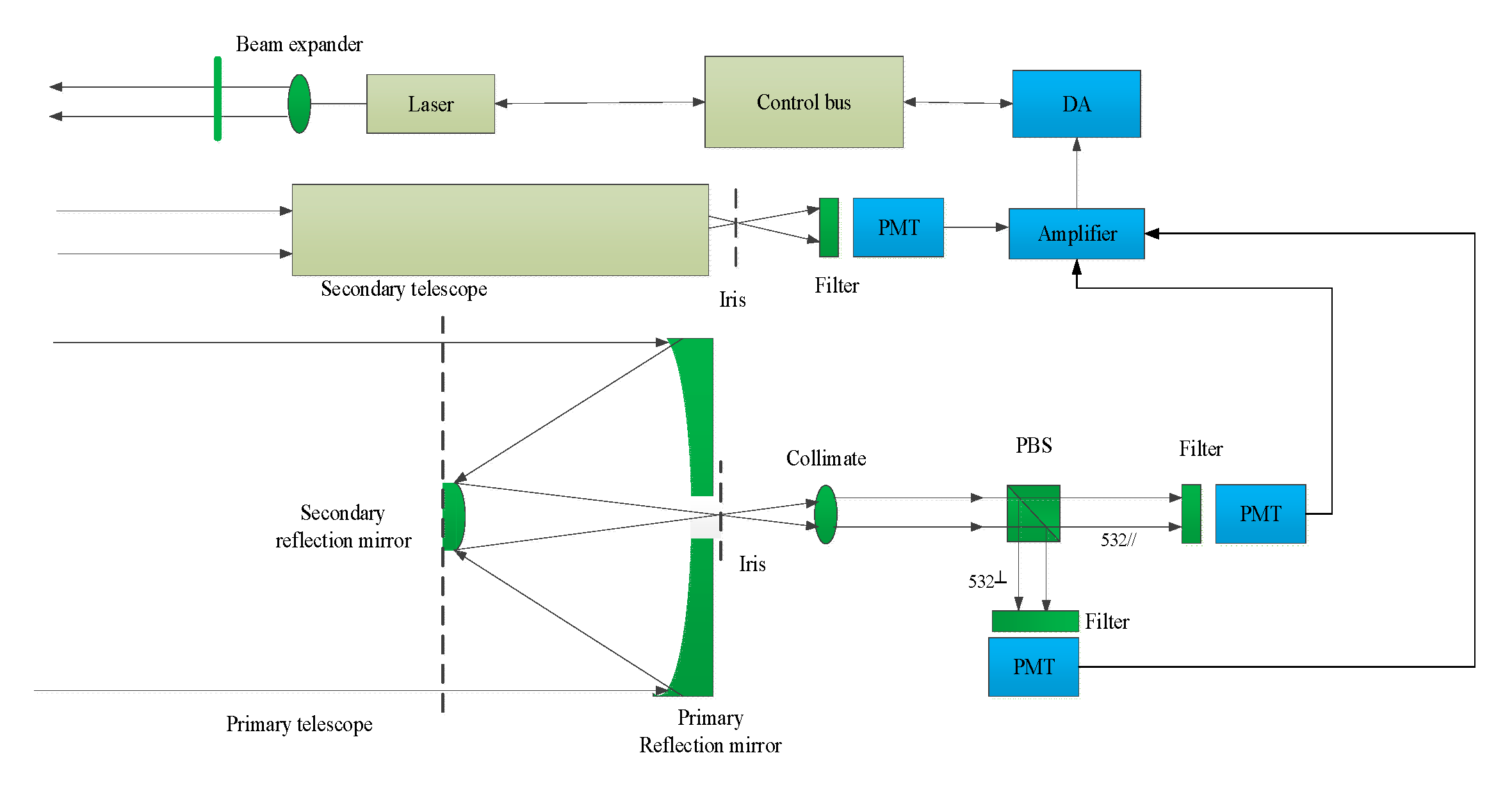
The system framework of the proposed dual-FOV lidar is shown in Figure 1. A homemade laser source provided a center wavelength of 532 nm and a fluctuation of ±0.3 nm. The single-pulse energy was 400 μJ. The repetition rate was 2–7 kHz. The linear-polarized laser beam has a divergence of 0.1 mrad collimated by a 10-times beam expander and shot into the air. The laser source with a green wavelength of 532 nm and a higher single-pulse energy from sophisticated commercial lasers was chosen to produce a higher signal-to-noise of observations and a less error of the extinction coefficients of aerosol.

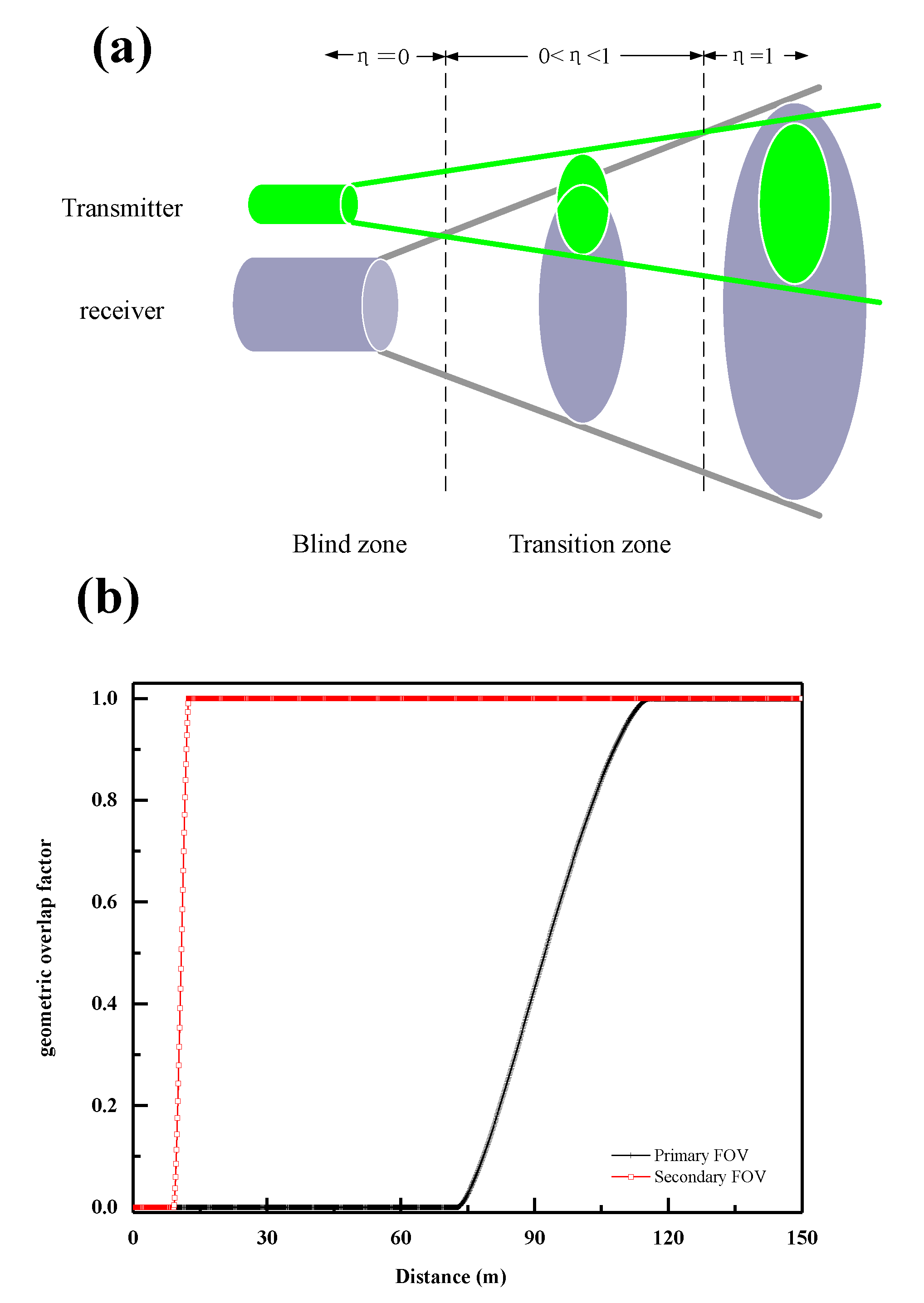
The primary FOV’s Mie backscattering signals were collected by a Cassegrain-type telescope, and the secondary FOV’s signals were collected by a Newtonian-type telescope at the same time. The primary telescope was designed with a diameter of 150 mm, a focal length of 700 mm, and an FOV of 1 mrad. The secondary telescope was designed with a diameter of 30 mm, a focal length of 118 mm, and an FOV of 8 mrad. A spacing of 25 mm was maintained between the optical axes of the two telescopes. The distances of the primary FOV optical axis and secondary FOV optical axis to the laser emitting axis were 121, and 58 mm, respectively. The intersection angle of the two optical axes was 0.2–0.4°. This intersection angle was adjustable and rather important to the performance of the lidar’s blind zone and transition zone. A typical GOF of the traditional dual-axis Mie-lidar is shown in Figure 2a and the calculated GOFs of the two FOVs of this lidar system are illustrated in Figure 2b. The GOF η of the lidar in Figure 2a depends on the parameters of the laser divergence angle, receiving FOV, and the distance between laser (transmitter) and receiving telescope. Within a very short distance from the lidar, the laser beam emitted by the laser does not receive in the telescope’s field of view. At this time, η = 0, and the receiving telescope cannot receive the atmospheric backscatter light. This area is called the blind zone of the lidar. Far away from the blind area, the emitted laser beam gradually enters the receiving field of view. Currently, η gradually increases from 0, but less than 1. The atmospheric backscattered light is only partially received. This area is called the transition zone of lidar. Far away from the transition region, the emitted laser beam is completely contained in the receiving field of view. At this time, there is always η = 1, and all the backscattered light in the atmosphere is received. From Figure 2b, it is demonstrated that a larger blind zone of about 75 m in primary FOV comparted with less than the 15 m of blind zone in the secondary FOV. It also illustrates that the transition zones of primary and secondary FOVs were 115.5, and 12.4 m, respectively. Here, we ignored the effects of the intersection angle of the secondary FOV in the GOF calculation.

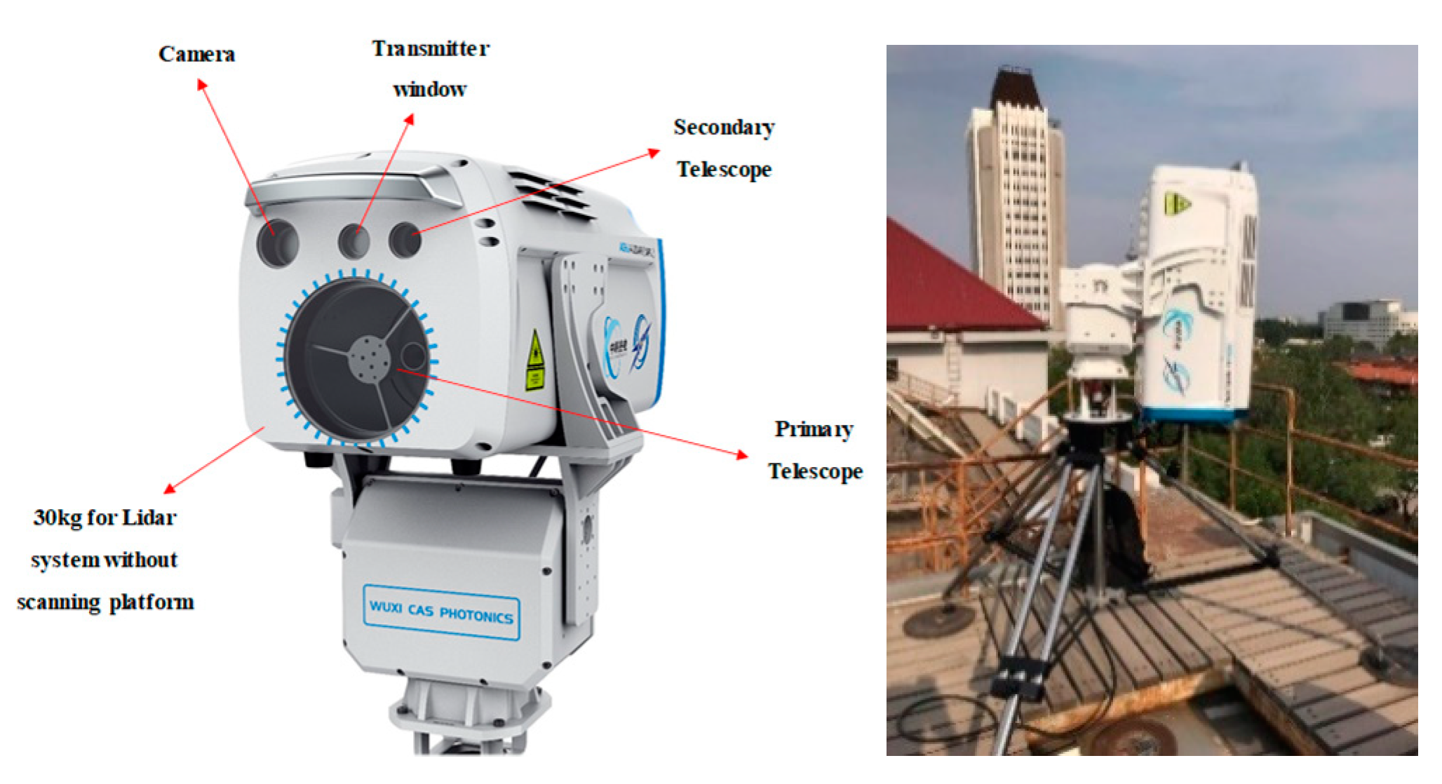
The polarized backscattered signals, collected by the primary FOV, traveled through an iris, a collimator, and a polarized beam splitter (PBS). After passing through the PBS, parallel and perpendicular signals went through two narrow-band filters with a bandwidth of 1.6 nm and an optical density of 5 to suppress the scattered light. The depolarization ratio was retrieved followed by the reference [14]. The signal in the secondary FOV passed through an iris and a narrow-band interference filter. All these three signals were detected by three photo multiplier tubes (PMTs). An amplifier and a 16-bit analog-to-digital converter were used to amplify and digitize the three-channel electrical signals. The data-acquisition rate was 20 MHz, and the transit time of PMTs was 2.7 ns. An industrial computer was embedded to save the raw data files. An outside view of the lidar, with detailed module identifications, is shown in Figure 3. The total weight of the lidar, including a scanning platform, which supports the three-dimensional (3-D) scanning of aerosols, was 65 kg. This portable lidar system is flexible for mobile applications and station observations.

2.2. Evaluation and Joining of the Signals from the Two FOVs

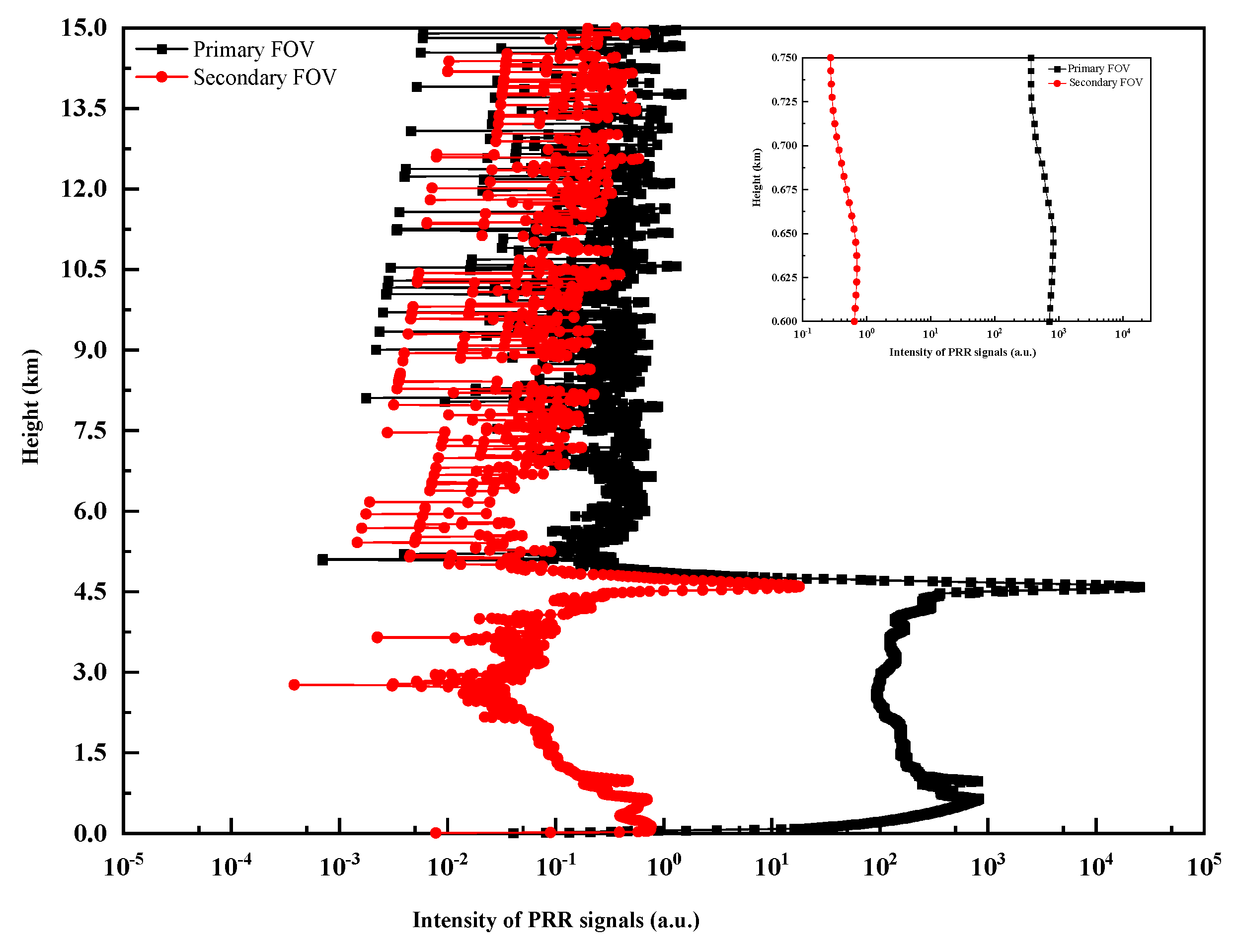
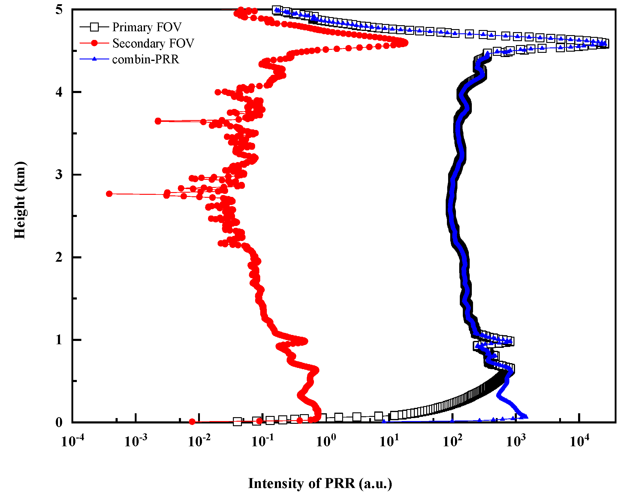
The backscattering range corrected signals (PRR), received by the two FOVs, are shown in Figure 4. The primary FOV’s signal (indicated by the black-square line in Figure 4) illustrated a higher signal-to-noise ratio (SNR) over 10 above 2 km. The strong intensity at 4.5 km referred to clouds. Many tiny peaks in the range of 0.75 km to approximately 4.5 km suggested more than 5 layers of aerosol distribution at the lower atmosphere. For the returned secondary FOV signal (red-dot line in Figure 4), a much higher SNR over 8 was shown below 2 km. Compared with the primary signal, sophisticated structures were clearly shown under 1 km.

To acquire a complete signal of dual FOV lidar, a careful joining evaluation of primary and secondary FOV signals was conducted thoroughly along the laser-beam path. An optimum combination interval with the most relevant linearity between the signals of the two fields was determined by the following Equation (1)

$$O\left(r\right)={\displaystyle \sum }_{i=m}^{m+∆n}{\left\{\left[a{P}_s\left(r\right)+b\right]-P_P\left(r\right)\right\}}^2$$

(1)

where O(r) is the square loss function of {P_s(r), P_p(r)} at the range of r. m is the joining start-point of the combination interval, Δn is the combination length, P_s(r) is the intensity of the PRR signal of the secondary FOV, and P_p(r) is the intensity of the PRR signal of the primary FOV. The intensity ratio of a and the slop of b will be determined by conducting a non-linear least square method.

A case is shown in Figure 4. Here, the combination interval was determined at 0.6~0.75 km (sub-chart in Figure 4), with a mean intensity ratio of 1212.7 and a minimum standard deviation of 29.2. The signal from the primary field over 0.75 km and the signal under 0.75 km from the secondary field corrected by the intensity ratio were composed to a complete return backscattering signal of the dual-FOV lidar. The original primary-field signal, the corrected secondary-field signal (multiplied by the intensity ratio), and the combined signal are illustrated in Figure 5. It is obvious that the combined signal retained excellent characteristics of the primary-field and secondary-field signals. In this way, the SNR of the entire signal exceeded 8, which was advantageous to inverse the extinction coefficients of aerosol. Although, different combination intervals will be different for every raw lidar signal, the combination length of 150 m was fixed in inversion procedure with a resolution of 7.5 m. In this lidar system, the signals’ joining start-points are always located below 1 km.

2.3. Evaluation of the Blind Zone and the Transition Zone of Dual-FOV Lidar

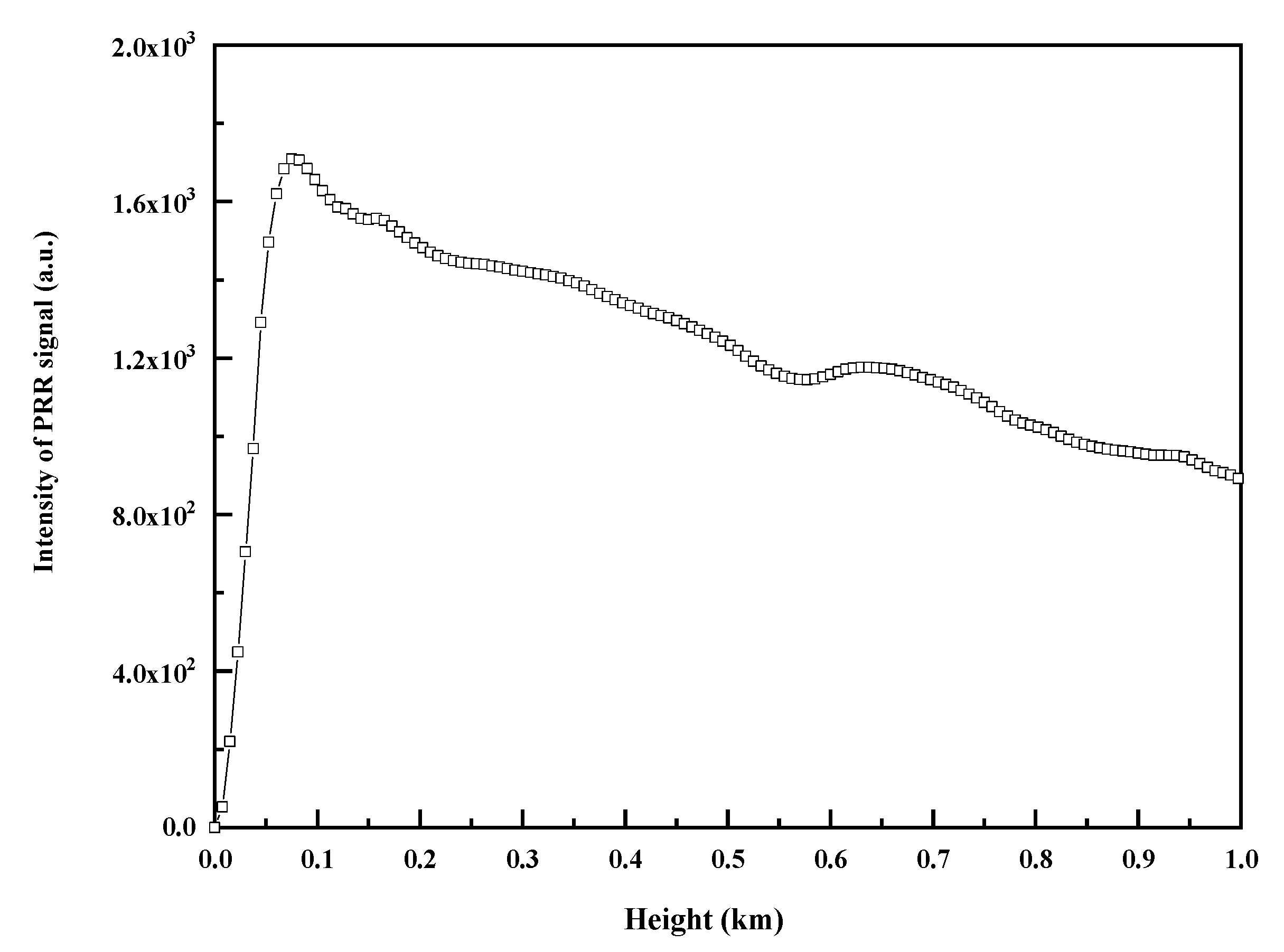
The blind zone and transition zone of this dual-FOV lidar system can be checked from the PRR of the secondary FOV. We aligned the laser beam parallel to the ground surface to measure the PRR signal, which is shown in Figure 6. This figure shows that the blind zone decreased to 0 m, and the transition zone was 60 m. This measured no-blind-zone was mainly due to the alignment of the intersection angle of the secondary FOV axis and the transmitter axis.

2.4. Retrieval of the Vertical Profile of Aerosols

The Fernald method [30,31], using the lidar equation given in Equation (2), was used to retrieve the vertical profile of aerosol extinction coefficients from the returned signals, which had been created by joining together the signals from the primary and secondary FOVs:

$$P\left(z\right)=\frac{C\cdot E\cdot \left[{\beta }_m\left(z\right)+{\beta }_a\left(z\right)\right]\cdot \exp \{-2{\int }_0^r\left[{\alpha }_m\left(z^{\prime }\right)+{\alpha }_a\left(z^{\prime }\right)\right]d{z}^{\prime }>\}}{z^2}.$$

(2)

Here, P(z) is the received power from altitude z. C is lidar system constant, E is the laser emitting pulse energy, and β_m(x) and β_a(z) are the backscattering coefficients of the atmosphere and aerosol at the range z, respectively. While, α_m(z) and α_a(z) are the atmospheric extinction coefficient and aerosol extinction coefficient at the range z, respectively.

2.5. Retrieval of Horizontal Distribution of Aerosols

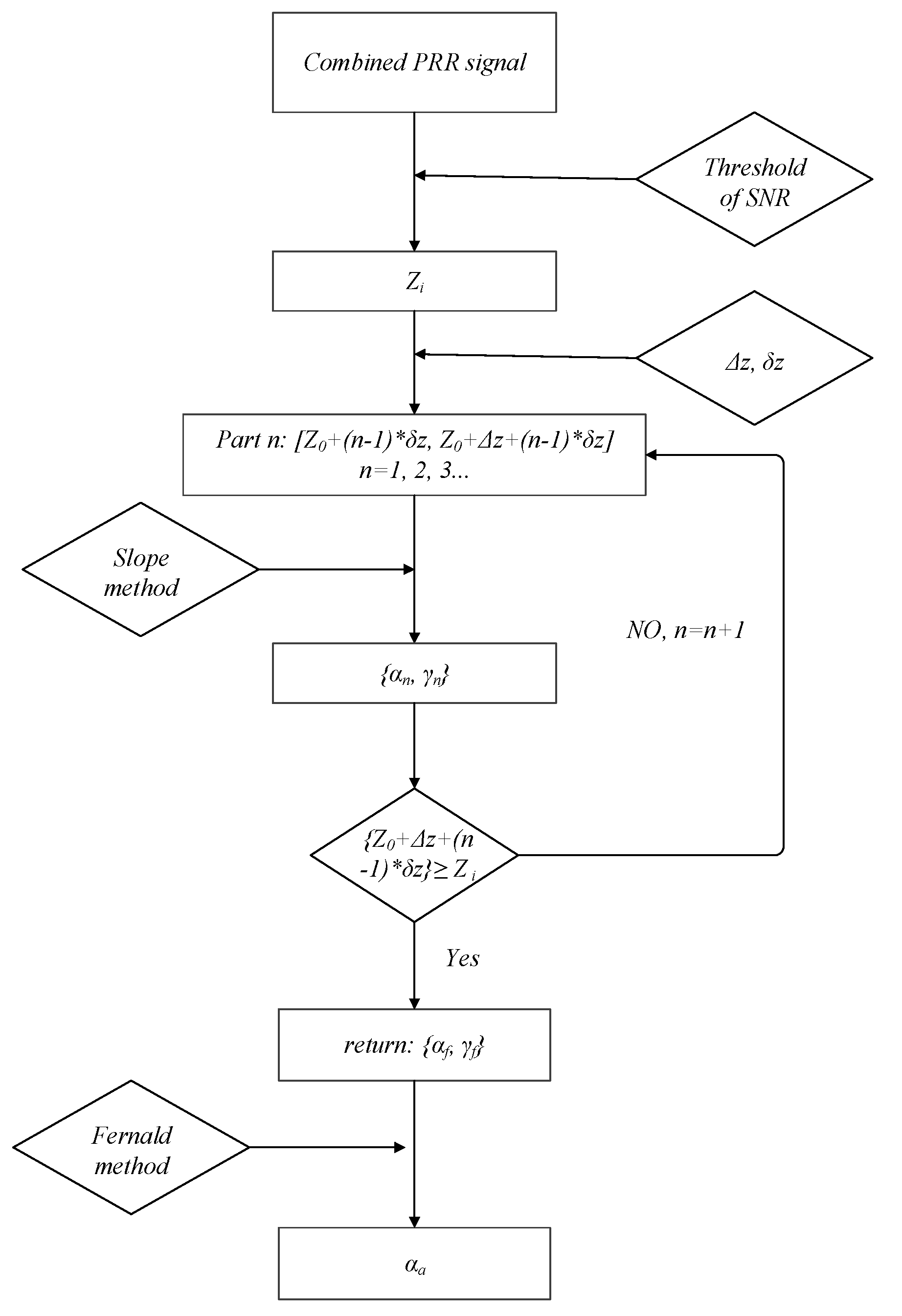
To implement the mapping of the near-surface aerosol level density distribution, a combination retrieval algorithm of the Fernald method and the slope method [32] was applied in the lidar Equation (2). The inversion procedure was as follows and the flow chart is illustrated in Figure 7.

• At an initial point Z_i, the position with an SNR that exceeds the threshold, along with each combined return signal, was determined;
• Then, the combined returned signal was divided into a series of parts from the origin point Z₀ to initial point Z_i as follows: part 1, Z₀~[Z₀ + Δz]; part 2, [Z₀ + δz]~[Z₀ + Δz + δz]; … part n, [Z₀ + (n − 1) × δz]~[Z₀ + Δz + (n − 1) × δz], etc., where n = 1, 2, …; Δz is the step of the interval and δz is the minimum spatial resolution of this lidar system;
• The slope method [32] was applied to each part. Pairs of both, aerosol extinction coefficients α_n and the Pearson coefficient γ_n were returned from each part;
• Finally, the pair of {α_f, Z_f} with the optimum γ_f was applied as boundary conditions in the Fernald solutions. The forward-integral and backward-integral results provide the entire profile of aerosol extinction coefficients in the horizontal distribution.

Here, the step of the interval Δz is closely related to the spatial resolution δz of the lidar system. In this study, an interval step of 75 m, which is 10 times δz, was chosen in the inversion procedure. The SNR threshold was chosen to be 5. The extinction-to-backscatter lidar ratio is an important factor for solving lidar Equation (2). A lidar ratio of 50, which is the representative value for continental aerosol detection at 532 nm, especially in eastern Asia [33,34], was applied in the lidar Equation (2).

3. Results and Discussion

3.1. Vertical Distribution Observation of Aerosols

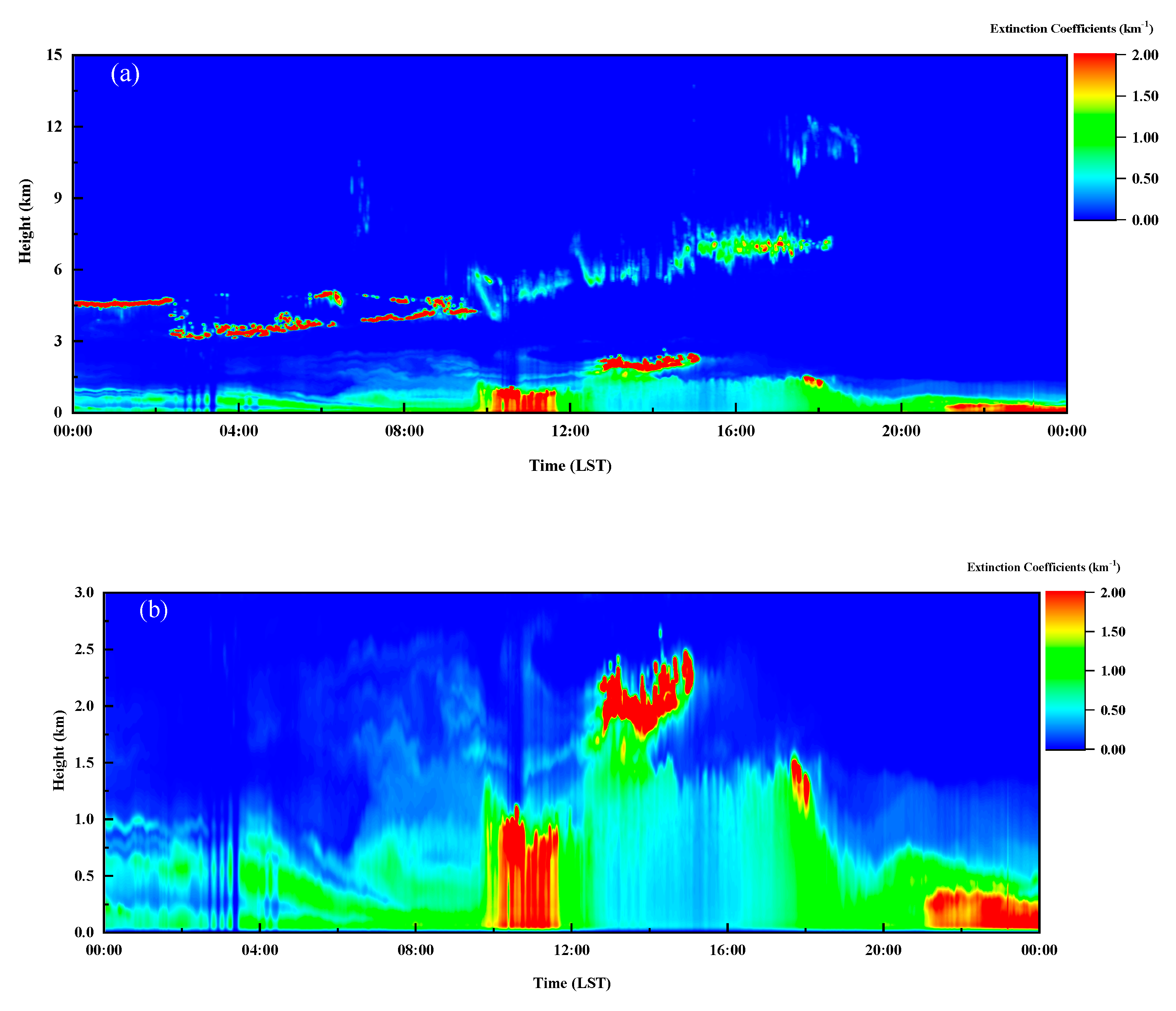
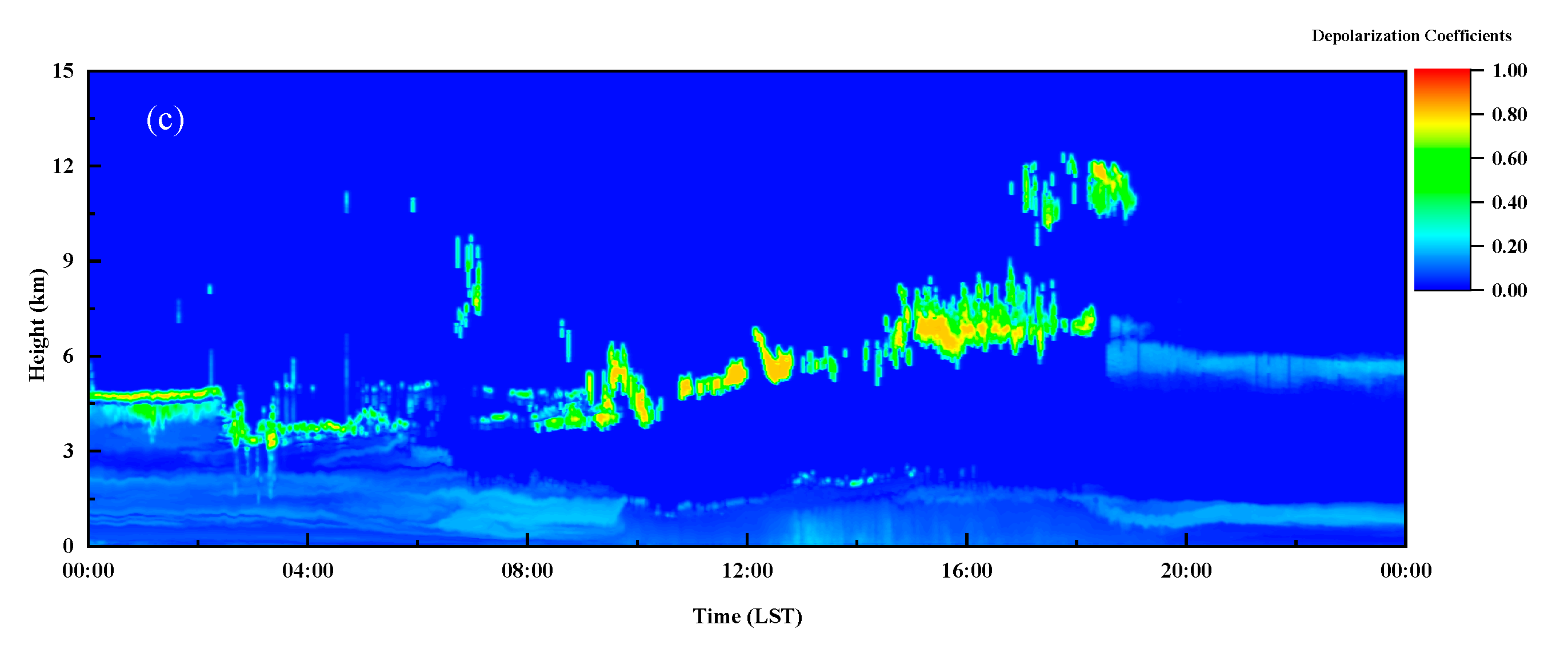
The vertical observation of aerosols with this dual-FOV lidar was performed on 14 April 2019, at Wuxi, Jiangsu, China. In the data analysis, the time coordinate used was local standard time (LST), which equates to coordinated universal time (UTC) +8 h. The lidar was set on the roof of an office building, which was approximately 30 m above ground level. A typical diurnal variation of the aerosol extinction coefficients is shown in Figure 8a. Aerosols were mainly distributed below 2 km in the early morning and night. The maximum extinction coefficient was close to 2 km⁻¹ and was observed after 22:00. During the daytime, the atmospheric boundary layer (ABL) increased from 1 km at 8:00 to 2.3 km at 13:00, and the ABL decreased to 800 m at 20:00. From 7:00. Transporting aerosol layers at 1.5~2.5 km were also detected, and these layers mixed with the boundary layer at noon, which increased the extinction coefficient to 1 km⁻¹. The maximum extinction coefficient reached 1.5 km⁻¹ at approximately 11:00. These tiny structures of aerosol distribution below 3 km are shown in Figure 8b. Cloud layers appeared from dawn to 18:00, with a spread range of 3~5 km, and the extinction coefficients are larger than 5 km⁻¹. Then, the extinction coefficients of clouds at noon decreased to approximately 2 km⁻¹. High-altitude clouds were also observed at 19:00 at 12 km. The depolarization observation from this lidar system is shown in Figure 8c. The depolarization ratio is significant to identify the aerosol types that include haze, dust, smoke, volcanic emissions, and particles released through pollution (e.g., carbon-based) or by the surface of the ocean, and those created by gas-to-particle conversions [14]. The aerosol distribution below 2.5 km had a depolarization ratio less than 0.15 mainly dominated by fine particles, and a depolarization ratio of more than 0.6 referred to the cloud distributions at 3~5 km and 12 km.

3.2. Horizontal Distribution Mapping of Aerosols

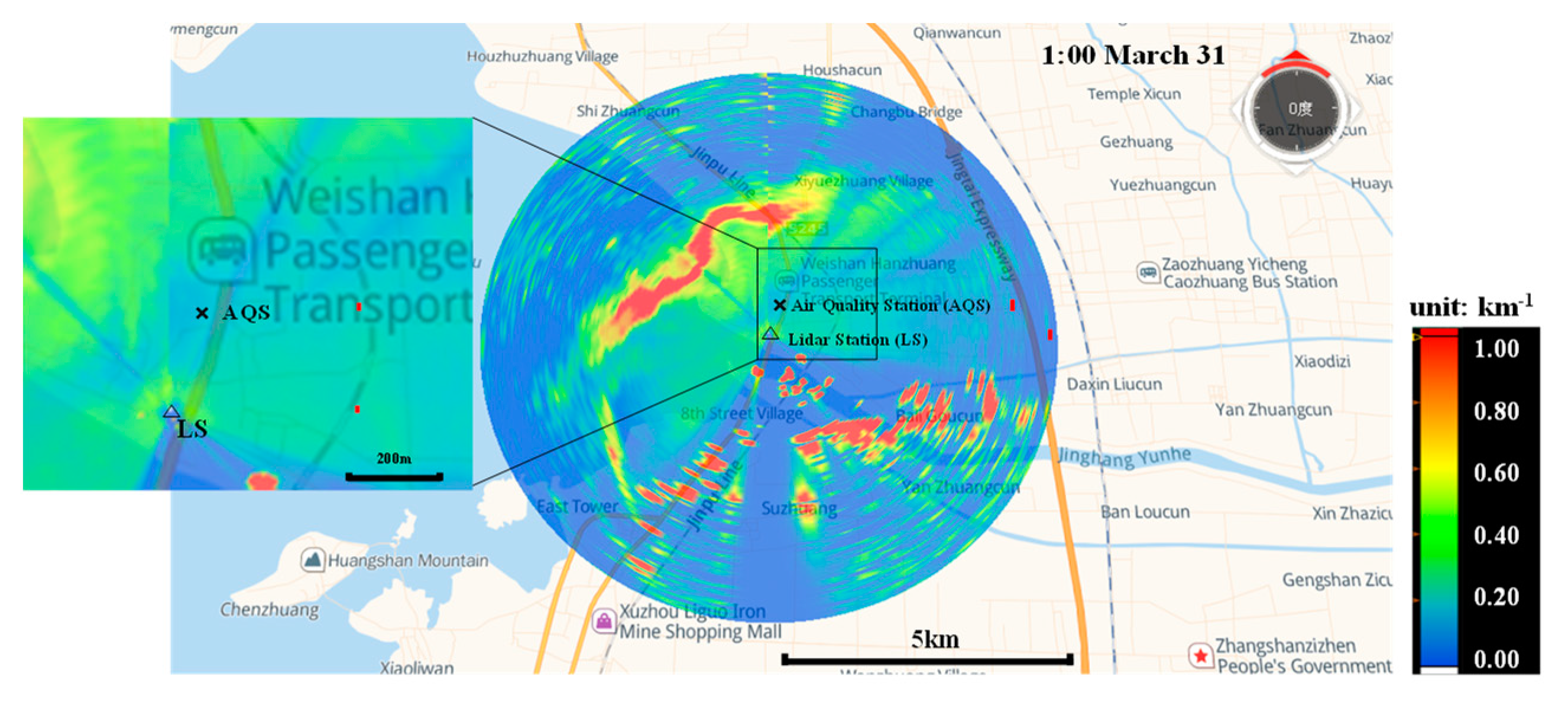
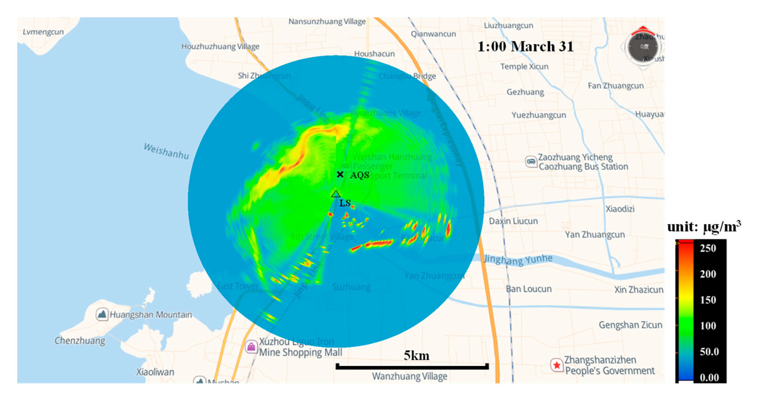
Field horizontal scanning experiments were conducted in the Shandong Province, China. The lidar station (LS) was set up on the roof of a primary school, which was 22 m above ground level in Hanzhuang Town, Jining City. Weishan Lake is located to the west of the LS. Some industrial plants are scattered on the south of the LS. Farmland is located at both, the north and the east of the LS. A national air quality station (AQS), Hanzhuang Station, is located 272 m northwest of the LS. This station provides in situ data of O₃, NO₂, SO₂, CO, PM₁₀ and PM_2.5. Meteorological parameters, i.e., the wind speed and wind direction, were also measured. The mass concentration of particulate matters ρ(PM₁₀) and ρ(PM_2.5) at the AQS were measured by TEOM™ (Thermo Scientific, Waltham, MA USA). The layout of the LS and AQS is shown in Figure 9.

The scanning parameters of the lidar system were set as follows. The elevation angle was fixed at 5°, and the azimuth angle was 0~360°. The repetition rate of the laser pulses was selected to be 7 kHz. The scanning angle resolution was 2°. Each returned signal was acquired with 150,000 times of the accumulation of the laser pulses. A total of 180 profiles were obtained for each cycle-scanning every 1.5 h. The scanned extinction coefficients of the aerosols were overlaid on the maps using a geo-information system (GIS).

One sample of aerosol distribution scanning on the early morning of 31 March is shown in Figure 9. It is noted that the aerosols were steadily suspended in the range of 2 km to the southwest, south and southeast of the LS. These areas are occupied by many large steel and iron factories and chemical plants. These pollution sources strongly contribute to the ρ(PM) at the AQS with a southeast wind direction. In Figure 9, a pollution mass with an approximate length of 5 km was observed 2~2.5 km north of the LS. The right-wing of this belt significantly influenced the ρ(PM) at the AQS. The corresponding ρ(PM₁₀) increased to 135 μg/m³ (Figure 10). The overhead extinction coefficient from the lidar system was 0.53 km⁻¹. This pollution mass led to air quality deterioration at AQS in the next few hours.

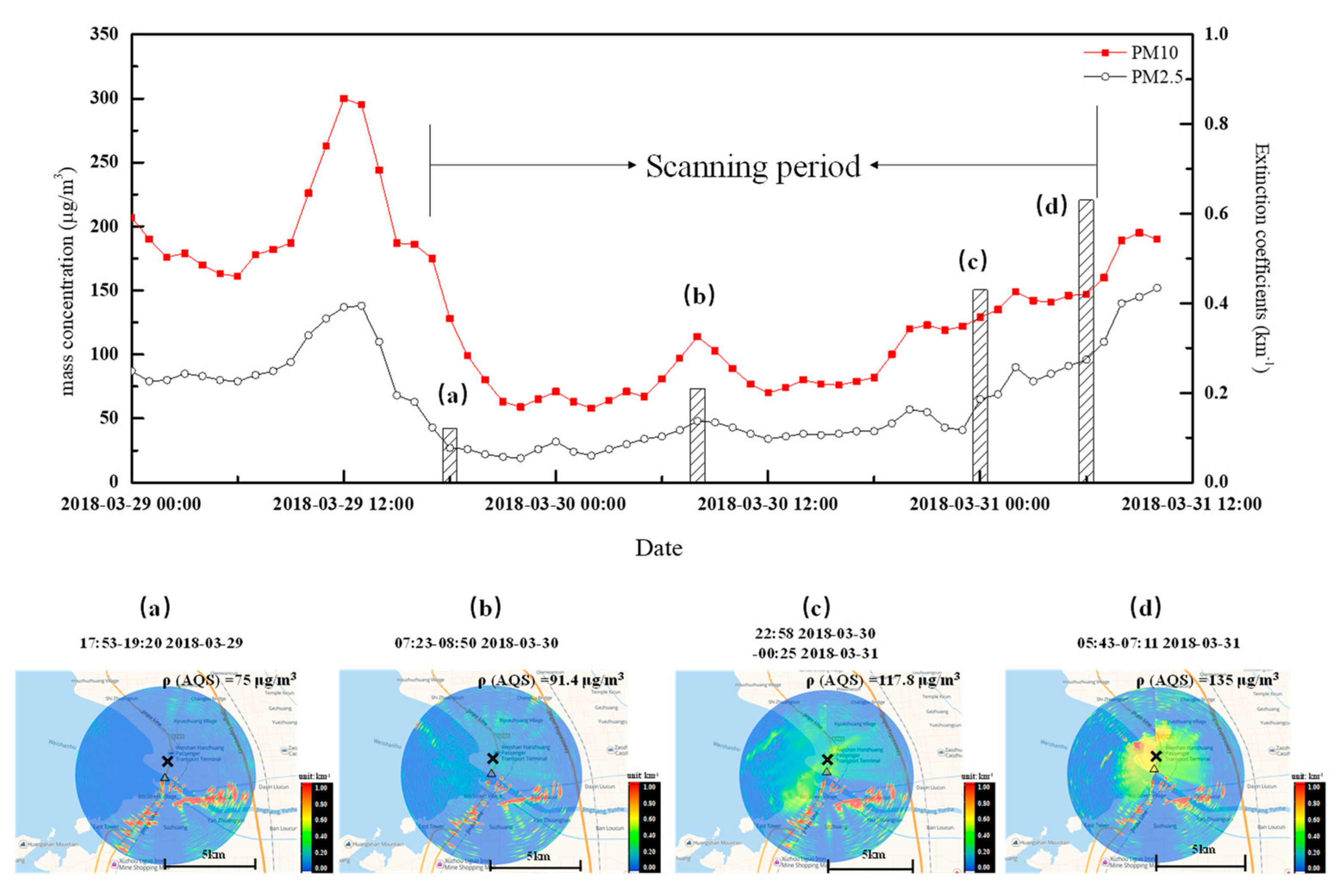
Lidar scanning began at 17:53, 29 March and ended at 07:11, 31 March 2018. In total, 30 cycle-scanning maps were acquired from this field experiment. Time series of ρ(PM) at the AQS and four lidar scanning results of aerosol distribution are shown in Figure 10. ρ(PM₁₀) and ρ(PM_2.5) decreased from 128 μg/m³, and 27 μg/m³, respectively, at the beginning of the observation (upper panel of Figure 10). The corresponding lidar scanning illustrated few particulate matters around the AQS, and the overhead extinction coefficient of the AQS was 0.12 km⁻¹ (lower panel Figure 10a). The ρ(PM₁₀) and ρ(PM_2.5) climbed up to 114 μg/m³ and 47.4 μg/m³ at 08:00, 30 March (upper panel of Figure 10). The lidar observation at 07:23–08:50 confirmed the accumulation of aerosols over the AQS, with an overhead extinction coefficient of 0.21 km⁻¹ (lower panel Figure 10b). From 23:00, 30 March, the ρ(PM₁₀) and ρ(PM_2.5) climbed steadily from 122 μg/m³ and 41 μg/m³ to 160 μg/m³, and 109 μg/m³, respectively, at 07:00, 31 March, the end of lidar scanning (upper panel of Figure 10). At this stage, the lidar maps show that the aerosols were enriched toward the AQS and increased the PM mass concentrations. The corresponding overhead extinction coefficients were 0.43 km⁻¹ at 23:00, 30 March and 0.63 km⁻¹ at 06:00, 31 March (lower panel Figure 10c,d).

3.3. Quantitative Evaluation of Aerosol Distribution

Mass concentration mapping of aerosols from the lidar system is an ideal choice for supporting environmental management, especially for air quality modeling simulations that rely on the following three advantages: (1) A higher spatial and temporal resolution of mass concentrations; (2) a greater observation range in both the vertical and horizontal directions; and (3) easy calibration, validation by an array of standard point instruments at ground level, and the establishment of a data set with data quality assurance.

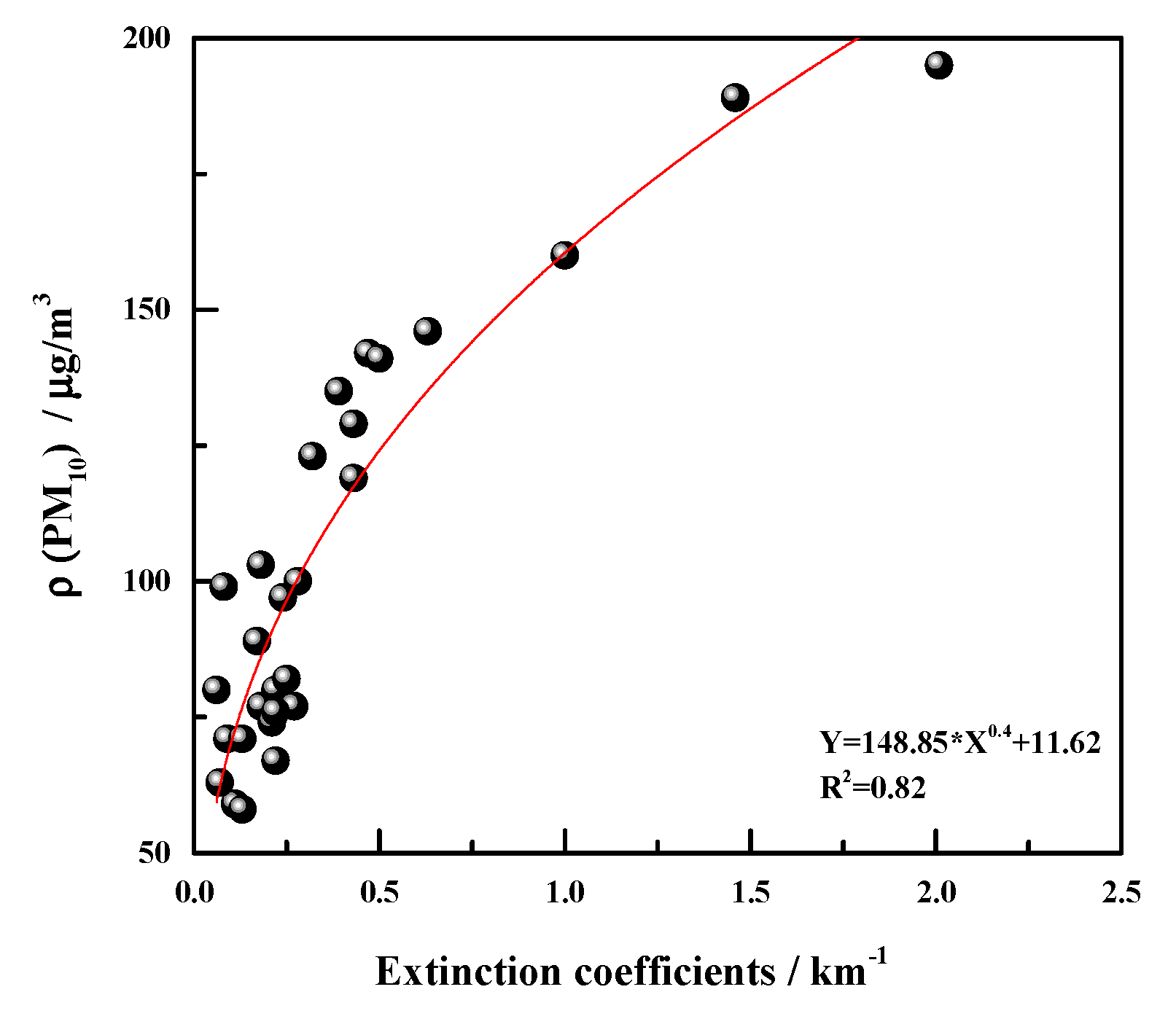
Here, a nonlinear relationship can be fitted with the ρ(PM₁₀) mass concentration at the AQS and the overhead extinction coefficients α_a from lidar scanning. This nonlinear relationship is shown as follows,

$$\rho \left(P{M}_{10}\right)=\kappa \cdot {\alpha }_a{}^{\zeta }+C$$

(3)

where κ, ζ, and C are the fitted parameters.

Using 30 sets of ρ(PM₁₀) and α_a values, the fitting relationship of Equation (3) is determined and is illustrated in Figure 11. The parameters are κ = 148.85 μg/m³, ζ = 0.4, and C = 11.62 μg/m³, and the Pearson coefficient is 0.91.

The lidar scanning results, the extinction coefficients of the aerosol distributions, can be transformed to aerosol mass concentration distributions with this fitted relationship. The early morning case on 31 March is shown again but with mass concentrations in Figure 12. The mass concentration of the point sources 2.5 km southeast of the LS was close to 250 μg/m³. The mass concentration of the “aerosol-belt” northwest of the LS exceeded 250 μg/m³. Figure 12 also ignored the low SNR regions of extinction coefficients, especially over the radius of 3 km. The calculated overhead mass concentrations of AQS were also illustrated in the lower panel in Figure 10. The overhead mass concentrations were 75 μg/m³ (99 μg/m³) at 19:00, 29 March, 91.4 μg/m³ (103 μg/m³) at 08:00, 30 March, 117.8 μg/m³ (129 μg/m³) at 00:00, 31 March, and 135 μg/m³ (147 μg/m³) at 19:00, 31 March, respectively. A difference from the ground sampling measurement from AQS (values in brackets) may be because of water vapor or relative humidity in Weishan Lake.

An accurate lidar ratio is important for the retrieval of extinction coefficients. In general, the lidar ratio varies with height and depends on the shape, size distribution and refractive index of the aerosol particles, as well as the lidar wavelength. Here, we applied a constant lidar ratio in the lidar equation for both the vertical and horizontal profile inversion. When we applied the “Fernald-slope” method to retrieve the horizontal distribution of aerosols, the SNR threshold was a critical definition. In the future, the effect of the SNR threshold will be discussed. It is noted that the lidar beam probed across the Weishan Lake surface, and a not negligible factor of water vapor was carefully considered when we converted the extinction coefficients to mass concentrations. The influence of the water vapor or the relative humidity on the retrieval of extinction coefficients has been studied by Zhao et al. [35], and the extinction coefficients here need to be carefully corrected in further studies. In addition, deploying a PM sampling array instead of a single lidar station and providing a few ρ(PM₁₀) and extinction coefficient datasets at different positions would be another reasonable measure to minimize the error of retrieving the mass concentration distribution. If possible, the chemical compositions of aerosols can be extracted to make a reasonable evaluation of the extinction coefficients.

4. Conclusions

A dual-FOV lidar was designed without a blind zone and a transition zone of 60 m to observe the lower atmosphere. Dual FOV technology was applied to overcome the traditional obstacles of Mie-lidars with hundreds of meters of blind zone. The lidar system is maneuverable and has a weight of less than 70 kg, including the scanning platform. A complete combined returned signal was acquired by carefully checking for the linear combination interval with the primary FOV signal and the secondary FOV signal. Vertical profiles of the aerosol field were retrieved with the Fernald method, while the horizontal distribution of aerosol extinction coefficients was retrieved by combining the slope method and the Fernald method. Horizontal scanning observations clearly showed the spatial-temporal distribution of aerosols. The lidar system can provide valuable and accurate pollution information with the mass concentration mapping, when validated with local quantitative PM measurements. Furthermore, the corrected mass concentration mapping data can be assimilated into 3-D air quality modeling, in order to significantly improve the accuracy of regional air quality predictions. This compact portable lidar system is also an ideal choice for the 3-D atmospheric stereo-pollution monitoring networks construction in severe polluted regions in the future, i.e., New Delhi in India, Beijing–Tianjin–Hebei (JJJ) in China, Bangkok in Southeast Asia.

References

- Liu, B.; Ma, Y.Y.; Gong, W.; Zhang, M.; Yang, J. Determination of boundary layer top on the basis of the characteristics of atmospheric particles. Atmos. Environ. 2018, 178, 140–147. [Google Scholar] [CrossRef]
- Han, S.Q.; Liu, J.L.; Hao, T.Y.; Zhang, Y.F.; Li, P.Y.; Yang, J.B.; Wang, Q.L.; Cai, Z.Y.; Yao, Q.; Zhang, M.; et al. Boundary layer structure and scavenging effect during a typical winter haze-fog episode in a core city of BTH region, China. Atmos. Environ. 2018, 179, 187–200. [Google Scholar] [CrossRef]
- Chen, Z.Y.; Liu, C.; Liu, W.Q.; Zhang, T.S.; Xu, J. A synchronous observation of enhanced aerosol and NO2 over Beijing, China, in winter 2015. Sci. Total Environ. 2017, 575, 429. [Google Scholar] [CrossRef] [PubMed]
- Pal, S.; Lee, T.R.; Phelps, S.; De Wekker, S.F.J. Impact of atmospheric boundary layer depth variability and wind reversal on the diurnal variability of aerosol concentration at a valley site. Sci. Total Environ. 2014, 496, 424–434. [Google Scholar] [CrossRef]
- Danchovski, V. Summertime Urban Mixing Layer Height over Sofia, Bulgaria. Atmosphere 2019, 10, 36. [Google Scholar] [CrossRef] [Green Version]
- Bozlaker, A.; Prospero, J.M.; Fraser, M.P.; Chellam, S. Quantifying the Contribution of Long-Range Saharan Dust Transport on Particulate Matter Concentrations in Houston, Texas, Using Detailed Elemental Analysis. Environ. Sci. Technol. 2013, 47, 10179–10187. [Google Scholar] [CrossRef]
- Salinas, S.V.; Chew, B.N.; Miettinen, J.; Campbell, J.R.; Welton, E.J.; Reid, J.S.; Yu, L.E.; Liew, S.C. Physical and optical characteristics of the October 2010 haze event over Singapore: A photometric and lidar analysis. Atmos. Res. 2013, 122, 555–570. [Google Scholar] [CrossRef]
- Xie, C.B.; Nishizawa, T.; Sugimoto, N.; Matstui, I.; Wang, Z.F. Characteristics of aerosol optical properties in pollution and Asian dust episodes over Beijing, China. Appl. Opt. 2008, 47, 4945–4951. [Google Scholar] [CrossRef]
- Nishizawa, T.; Sugimoto, N.; Matsui, I.; Shimizu, A.; Hara, Y.; Itsushi, U.; Yasunaga, C.; Kudo, R.; Kim, S.W. Ground-based network observation using Mie–Raman lidars and multi-wavelength Raman lidars and algorithm to retrieve distributions of aerosol components. J. Quant. Spectrosc. RA 2017, 188, 79–93. [Google Scholar] [CrossRef]
- Matthais, V.; Freudenthaler, V.; Amodeo, A.; Balin, I.; Balis, D.; Bӧsenberg, J.; Chaikovsky, A.; Chourdakis, G.; Comeron, A.; Delaval, A.; et al. Aerosol lidar intercomparison in the framework of the EARLINET project. 1. Instruments. Appl. Opt. 2004, 43, 961–976. [Google Scholar] [CrossRef]
- Chiang, C.W.; Das, S.K.; Chiang, H.W.; Nee, J.B.; Sun, S.H.; Chen, S.W.; Lin, P.H.; Chu, J.C.; Su, C.S.; Su, L.S. A new mobile and portable scanning lidar for profiling the lower troposphere. Geosci. Instrum. Meth. 2015, 4, 35–44. [Google Scholar] [CrossRef]
- Chazette, P.; Sanak, J.; Dulac, F. New Approach for Aerosol Profiling with a Lidar Onboard an Ultralight Aircraft: Application to the African Monsoon Multidisciplinary Analysis. Environ. Sci. Technol. 2007, 41, 8335–8341. [Google Scholar] [CrossRef] [PubMed]
- Proestakis, E.; Amiridis, V.; Marinou, E.; Georgoulias, A.K.; Solomos, S.; Kazadzis, S.; Chimot, J.; Che, H.Z.; Alexandri, G.; Binietoglou, I.; et al. 9-year spatial and temporal evolution of desert dust aerosols over South-East Asia as revealed by CALIOP. Atmos. Chem. Phys. 2018, 18, 1–35. [Google Scholar] [CrossRef] [Green Version]
- Weitkamp, C. LIDAR: Range-Resolved Optical Remote Sensing of the Atmosphere; Springer: New York, NY, USA, 2004. [Google Scholar]
- Kovalev, V.A.; Eichinger, W.E. Elastic Lidar: Theory, Practice, and Analysis Methods; Wiley-Interscience: New York, NY, USA, 2004. [Google Scholar]
- Sasano, Y.; Shimizu, H.; Takeuchi, N.; Okuda, M. Geometrical form factor in the laser radar equation: An experimental determination. Appl. Opt. 1979, 18, 3908–3910. [Google Scholar] [CrossRef] [PubMed]
- Kuze, H.; Kinjo, H.; Sakurada, Y.; Takeuchi, N. Field-of-view dependence of lidar signals by use of Newtonian and Cassegrainian telescopes. Appl. Opt. 1998, 37, 3128–3132. [Google Scholar] [CrossRef]
- Welton, E.J.; Voss, K.J.; Gordon, H.R.; Maring, H.; Smirnov, A.; Holben, B.; Schmid, B.; Livingston, J.M.; Russell, P.B.; Durkee, P.A.; et al. Ground-based lidar measurements of aerosols during ACE-2: Instrument description, results, and comparisons with other ground-based and airborne measurements. Tellus B 2000, 52, 636–651. [Google Scholar] [CrossRef] [Green Version]
- Stelmaszczyk, K.; Dell’Aglio, M.; Chudzyński, S.; Stacewicz, T.; Wöste, L. Analytical function for lidar geometrical compression form-factor calculations. Appl. Opt. 2005, 44, 1323–1331. [Google Scholar] [CrossRef]
- Hey, J.V.; Coupland, J.; Foo, M.H.; Richards, J.; Sandford, A. Determination of overlap in lidar systems. Appl. Opt. 2011, 50, 5791–5797. [Google Scholar]
- He, T.Y.; Stanič, S.; Gao, F.; Bergant, K.; Veberič, D.; Song, X.Q.; A. Dolžan, A. Tracking of urban aerosols using combined lidar-based remote sensing and ground-based measurements. Atmos. Meas. Tech. 2012, 5, 891–900. [Google Scholar] [CrossRef] [Green Version]
- Behrendt, A.; Pal, S.; Wulfmeyer, V.; Valdebenito, B.Á.M.; Lammel, G. A novel approach for the characterization of transport and optical properties of aerosol particles near sources—Part I: Measurement of particle backscatter coefficient maps with a scanning UV lidar. Atmos. Environ. 2011, 45, 2795–2802. [Google Scholar] [CrossRef]
- Sasano, Y. Tropospheric aerosol extinction coefficient profiles derived from scanning lidar measurements over Tsukuba, Japan, from 1990 to 1993. Appl. Opt. 1996, 35, 4941–4952. [Google Scholar] [CrossRef] [PubMed] [Green Version]
- Shan, H.H.; Zhang, H.; Liu, J.J.; Tao, Z.M.; Wang, S.H.; Ma, X.M.; Zhou, P.C.; Yao, L.; Liu, D.; Xie, C.B.; et al. Retrieval method of aerosol extinction coefficient profile based on backscattering, side-scattering and Raman-scattering lidar. Opt. Commun. 2018, 410, 730–732. [Google Scholar] [CrossRef]
- Bian, Y.X.; Zhao, C.S.; Xu, W.Y.; Kuang, Y.; Tao, J.C.; Wei, W.; Ma, N.; Zhao, G.; Lian, S.P.; Tan, W.S.; et al. A novel method to retrieve the nocturnal boundary layer structure based on CCD laser aerosol detection system measurements. Remote Sens. Environ. 2018, 211, 38–47. [Google Scholar] [CrossRef]
- Barnes, J.E.; Parikh, N.C.; Kaplan, T. Boundary layer scattering measurements with a charge-coupled device camera lidar. Appl. Opt. 2003, 42, 2647–2652. [Google Scholar] [CrossRef]
- Meki, K.; Yamaguchi, K.; Li, X.; Saito, Y.; Kawahara, T.D.; Nomura, A. Range-resolved bistatic imaging lidar for the measurement of the lower atmosphere. Opt. Lett. 1996, 21, 1318–1320. [Google Scholar] [CrossRef] [PubMed]
- Schmidt, J.; Wandinger, U.; Malinka, A. Dual-field-of-view Raman lidar measurements for the retrieval of cloud microphysical properties. Appl. Opt. 2013, 52, 2235–2247. [Google Scholar] [CrossRef] [PubMed]
- Gong, W.; Li, J.; Mao, F.Y.; Zhang, J.Y. Comparison of simultaneous signals obtained from a dual-field-of-view lidar and its application to noise reduction based on empirical mode decomposition. Chin. Opt. Lett. 2011, 9, 050101. [Google Scholar] [CrossRef]
- Fernald, F.G. Analysis of atmospheric lidar observations- Some comments. Appl. Opt. 1984, 23, 652–653. [Google Scholar] [CrossRef] [PubMed]
- Fernald, F.G.; Herman, B.M.; Reagan, J.A. Determination of Aerosol Height Distributions by Lidar. J. Appl. Meteorol. 1972, 11, 482–489. [Google Scholar] [CrossRef] [Green Version]
- Collis, R.T.H. Lidar: A new atmospheric probe. Q. J. R. Meteor. Soc. 1966, 92, 220–230. [Google Scholar] [CrossRef]
- Chiang, C.W.; Das, S.K.; Nee, J.B. An iterative calculation to derive extinction-to-backscatter ratio based on lidar measurements. J. Quant. Spectrosc. R. 2008, 109, 1187–1195. [Google Scholar] [CrossRef]
- Müller, D.; Ansmann, A.; Mattis, I.; Tesche, M.; Wandinger, U.; Althausen, D.; Pisani, G. Aerosol-type-dependent lidar ratios observed with Raman lidar. J. Geophys. Res. 2007, 112, D16202. [Google Scholar] [CrossRef]
- Zhao, G.; Zhao, C.; Kuang, Y.; Tao, J.; Tan, W.; Bian, J.; Li, C. Impact of aerosol hygroscopic growth on retrieving aerosol extinction coefficient profiles from elastic-backscatter lidar signals. Atmos. Chem. Phys. 2017, 17, 12133–12143. [Google Scholar] [CrossRef] [Green Version]
Figure 1.
Systematic framework of the dual-field-of-view (FOV) laser detection and ranging (lidar).
Figure 2.
(a) The typical geometric overlap factor (GOF) of the traditional dual-axis Mie-lidar and (b) the calculated GOFs of primary and secondary FOVs. The effects of the intersection angle were ignored in the calculation of the secondary FOV.
Figure 3.
Outside-view of dual-FOV lidar. Front view of dual FOV lidar (left) and field-experiment view of dual FOV lidar (right).
Figure 4.
Intensities of backscattering range-corrected signals (PRR) from primary FOV (black square line) and secondary FOV (red dot line). A case of the primary (black square line) and secondary FOV PRR signal (red dot line) at the combining region of 0.6~0.75 km is shown in the sub-chart.
Figure 5.
Intensities of combined PRR signal (blue triangle line), primary FOV PRR signal (black square line), and secondary FOV PRR signal (red dot line) of dual-FOV lidar.
Figure 6.
Evaluation of the blind zone and transition zone in dual FOV lidar with the parallel returned PRR signal of secondary FOV.
Figure 7.
Flow chart of inversion procedure of dual-FOV lidar. Zi is the initial position, whose SNR exceeds the threshold. Δz is the step of the interval and δz is the minimum spatial resolution of this lidar system. {αn, γn} are the aerosol extinction coefficients inversed by the slope method and the Pearson coefficient at part n. {αf, γf} are the optimum aerosol extinction coefficients with the maximum Pearson coefficient at part f. αa is the extinction coefficient of the aerosol profile inversed by the Fernald method.
Figure 8.
Vertical profile of aerosol detected by dual-FOV lidar. (a) Aerosol extinction coefficients in 15 km. (b) Aerosol extinction coefficients in 3 km. (c) The depolarization coefficients at 532 nm on 14 April 2019.
Figure 9.
Horizontal extinction coefficient distribution of aerosols at 1:00, 31 March. Sub-chart illustrated the aerosol distribution in the region between lidar station (LS) and air quality station (AQS) on 31 March. (Δ, the position of LS. ×, the position of AQS).
Figure 10.
Time series of ρ(PM10), ρ(PM2.5) of the air quality station (AQS), and the overhead extinction coefficients of AQS from lidar (upper panel) and the aerosol mappings from lidar at Hanzhuang at 17:53–19:20, 29 March (lower pane (a)), 07:23–08:50, 30 March (lower pane (b)), 22:58, 30 March–00:25, 31 March (lower pane (c)), and 05:43–07:11, 31 March (lower pane (d)) (Δ, the position of lidar, LS. ×, the position of AQS).
Figure 11.
Fitting result with extinction coefficients and ρ(PM10).
Figure 12.
Level mass concentration distribution of aerosols at 1:00, 31 March, of dual-FOV lidar (at altitude of 22 m). (Δ, the position of lidar, LS. ×, the position of air quality station, AQS).
© 2020 by the authors. Licensee MDPI, Basel, Switzerland. This article is an open access article distributed under the terms and conditions of the Creative Commons Attribution (CC BY) license (http://creativecommons.org/licenses/by/4.0/).
Share and Cite
MDPI and ACS Style
Wang, J.; Liu, W.; Liu, C.; Zhang, T.; Liu, J.; Chen, Z.; Xiang, Y.; Meng, X. The Determination of Aerosol Distribution by a No-Blind-Zone Scanning Lidar. Remote Sens. 2020, 12, 626. https://0-doi-org.brum.beds.ac.uk/10.3390/rs12040626
AMA Style
Wang J, Liu W, Liu C, Zhang T, Liu J, Chen Z, Xiang Y, Meng X. The Determination of Aerosol Distribution by a No-Blind-Zone Scanning Lidar. Remote Sensing. 2020; 12(4):626. https://0-doi-org.brum.beds.ac.uk/10.3390/rs12040626
Chicago/Turabian StyleWang, Jie, Wenqing Liu, Cheng Liu, Tianshu Zhang, Jianguo Liu, Zhenyi Chen, Yan Xiang, and Xiaoyan Meng. 2020. "The Determination of Aerosol Distribution by a No-Blind-Zone Scanning Lidar" Remote Sensing 12, no. 4: 626. https://0-doi-org.brum.beds.ac.uk/10.3390/rs12040626
Note that from the first issue of 2016, this journal uses article numbers instead of page numbers. See further details here.