Article

Efficient Discrimination and Localization of Multimodal Remote Sensing Images Using CNN-Based Prediction of Localization Uncertainty

1
Department of Information-Communication Technologies, National Aerospace University, 61070 Kharkiv, Ukraine
2
IETR UMR CNRS 6164, University of Rennes 1, Enssat, 22305 Lannion, France
*
Author to whom correspondence should be addressed.
Submission received: 28 January 2020 / Revised: 16 February 2020 / Accepted: 17 February 2020 / Published: 20 February 2020
(This article belongs to the Section Remote Sensing Image Processing)

Abstract

:
Detecting similarities between image patches and measuring their mutual displacement are important parts in the registration of multimodal remote sensing (RS) images. Deep learning approaches advance the discriminative power of learned similarity measures (SM). However, their ability to find the best spatial alignment of the compared patches is often ignored. We propose to unify the patch discrimination and localization problems by assuming that the more accurately two patches can be aligned, the more similar they are. The uncertainty or confidence in the localization of a patch pair serves as a similarity measure of these patches. We train a two-channel patch matching convolutional neural network (CNN), called DLSM, to solve a regression problem with uncertainty. This CNN inputs two multimodal patches, and outputs a prediction of the translation vector between the input patches as well as the uncertainty of this prediction in the form of an error covariance matrix of the translation vector. The proposed patch matching CNN predicts a normal two-dimensional distribution of the translation vector rather than a simple value of it. The determinant of the covariance matrix is used as a measure of uncertainty in the matching of patches and also as a measure of similarity between patches. For training, we used the Siamese architecture with three towers. During training, the input of two towers is the same pair of multimodal patches but shifted by a random translation; the last tower is fed by a pair of dissimilar patches. Experiments performed on a large base of real RS images show that the proposed DLSM has both a higher discriminative power and a more precise localization compared to existing hand-crafted SMs and SMs trained with conventional losses. Unlike existing SMs, DLSM correctly predicts translation error distribution ellipse for different modalities, noise level, isotropic, and anisotropic structures.

Graphical Abstract

1. Introduction

A popular strategy for solving the image registration problem involves two steps: finding a set of putative correspondences (PC) between patches of registered images and estimating geometrical transform parameters between these images on basis of the found PCs [1,2]. The basic element of this strategy is detecting similarity between two image patches and finding the exact spatial alignment between them. Therefore, two features of an SM are of equal importance in RS: the ability to distinguish similar and dissimilar pairs of patches and the ability to accurately estimate the position alignment of the compared patches. In RS, subpixel localization accuracy is a prerequisite for reaching high accuracy of image registration [3]. This problem has the highest complexity for multimodal images, when the compared patches are acquired with sensors of different physical nature, e.g., an optical sensor working in visual and infrared spectrum range [4,5,6], a radar sensor, a LIDAR, or even a Digital Elevation Model (DEM) [1]. Following existing terminology, the problem of finding similarity between two image patches will be called patch matching.
A number of SMs were proposed for patch matching over the last decades [7]. Area-based methods apply a complex decision rule that is robust to the structural difference between the compared pair of patches. In feature-based methods, the decision rule is reduced to comparing the value of an appropriate measure to a threshold (usually the sum of squared differences (SSD) or normalized correlation coefficient (NCC)), but the compared patches are first converted in a complex way into an invariant representation called a characteristic (feature) vector [8]. A group of area-based SMs stems from statistical or informational approaches including NCC [9], Phase Correlation [10], Mutual Information (MI) [11], and model-based maximum likelihood approach [12]. The drawback of area-based SMs is lack of robustness to structural changes in the compared patches [13]. Hand-crafted descriptors are designed to overcome this limitation, for example the widely used Scale-Invariant Feature Transform (SIFT) [14]. Among descriptors found useful for multimodal image registration, we would like to mention a version of SIFT specially adapted for radar images, SIFT-OCT [15], Histogram of Orientated Phase Congruency (HOPC) [13], and Modality Independent Neighborhood Descriptor (MIND) [16].
Deep Learning is an emerging and promising technique for designing efficient SMs in Computer Vision [17,18,19,20], Medical Imaging [21,22], and Remote Sensing [23,24]. The discriminative power of learned SMs is a topic under active research, and it already exceeds that of hand-crafted SMs by a significant margin. However, the accuracy of their localization power is still an open problem. We will review existing learned SMs in the next section.
Our contribution to the patch matching problem is a novel convolutional neural network (CNN), called Deep Localization Similarity Measure (DLSM). It is designed for improving both discrimination power and localization accuracy compared to existing hand-crafted and learned SMs. Patch discrimination and localization are not addressed as different problems, but rather as two aspects of the same problem. We speculate that similar patches are easier to localize and vice versa. To corroborate this hypothesis, let us consider a specific class of image patches that can be modeled as correlated samples of isotropic fractal Brownian motion field, as done in [25]. The main factors identified as affecting the theoretically predicted localization accuracy of such image patches are signal-to-noise ratio (SNR) for the reference and template patches (RP and TP) and NCC between them. The same factors also influence the discrimination between patches. For low SNR, detecting similarity between patches becomes more difficult. NCC by itself is a well-known and widely used similarity measure. This example is valid for the specific class of patches. In this work, we exploit the same idea for more complex patch situations with structural differences as well as isotropic and anisotropic structures.
DLSM takes a pair of the input patches, predicts the translation vector between them, and simultaneously predicts a 2 by 2 covariance matrix of the translation vector prediction error. The localization of the patch pair is characterized by the determinant of the expected covariance matrix (area of the deviation ellipse of the predicted translation vector). This determinant acts as a measure of similarity between the input patches, i.e., the decision on the similarity of the patches is made if the covariance matrix determinant takes a value below a predefined threshold. To achieve a high value for both the discrimination power and localization accuracy, the proposed CNN is trained with a mixed loss function comprising two terms. The first term is the log-likelihood of the two-dimensional normal distribution of the prediction error of the translation vector. This term expresses the estimation of translation as a deep regression with uncertainty problem. The second term is the triplet ratio loss applied to the values of the determinant of the covariance matrix for the positive and negative samples. It contributes to improving the discrimination power of the learned SM. The mixed loss transforms the patch matching problem from initially a pure binary classification problem to a classification–regression problem.
Experiments on a large set of multimodal images show that DLSM simultaneously improves the quality of discrimination and accuracy of patch localization. An important feature, which is lacking in existing SMs, is that the localization accuracy is predicted for each pair of patches, including isotropic and anisotropic textures, patches with low and high SNR, and patches with different modalities in the form of an error covariance matrix. This value can be used advantageously to set a proper PC weighting during multimodal image registration [1,2,26].
This paper is organized as follows. Section 2 reviews existing learned SMs. Section 3 introduces requirements and performance criteria for assessing SMs in remote sensing. Then, the CNN structure and loss function for learning an SM with high discriminative power and high localization accuracy are described in detail. Section 4 compares the proposed DLSM SM with existing hand-crafted SMs and learned SMs with conventional loss functions. Finally, conclusions and remarks on future work are given in Section 5.

2. Related Work

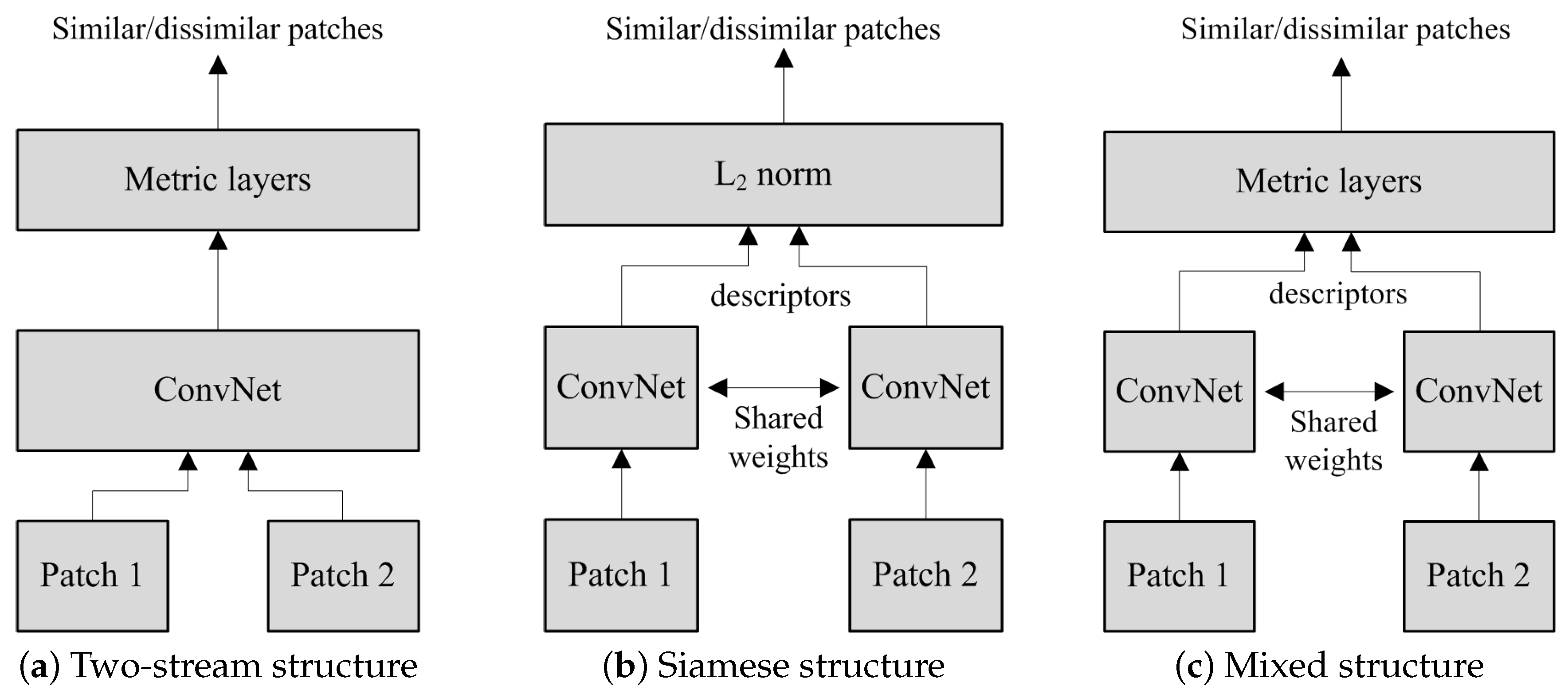
2.1. Overview of Existing Patch Matching CNN Structure and Loss Functions

The distinction between the two general types of CNN for patch matching, i.e., CNNs with and without metric learning [27] is similar to the distinction between area-based and feature-based SMs. Similarly to area-based methods, CNNs with metric learning (Figure 1a) compare a pair of patches jointly, whereas CNNs without metric learning or descriptor CNNs (Figure 1b) calculate a feature vector for each patch in the pair separately as in the case of feature-based SMs.
CNNs with metric learning are typically implemented as a two-stream CNN, whereas descriptor CNNs are trained using a Siamese architecture [18]. Mixed architectures are a compromise between the two-stream and Siamese architectures, where feature extraction is done by a Siamese CNN first, and evaluation of the metric by a two-stream CNN (Figure 1c) [4,28,29].
CNNs with metric learning are considered to have better accuracy [27] at the expense of a higher computational complexity. In descriptor CNNs, the most computationally complex part of the calculation of the feature vector, thereafter used to compare patches, is applied to individual patches, whereas the comparison is made with all patch pairs using a metric learning CNN.
Simo-Serra et al. utilized a Siamese network architecture for training a descriptor CNN that extracts 128-D descriptors whose euclidean distances reflect patch similarity [30]. As a step forward, Han et al. proposed a CNN denoted MatchNet representing a feature vector extraction CNN followed by a feature vector matching CNN or metric network [28]. The metric network comprising three fully connected (FC) layers aims to substitute simpler metrics for the comparison of feature vectors such as SSD or NCC. The MatchNet mixes Siamese and two-stream architectures for feature extraction and metric learning stages. The TS-Net CNN proposed in [4] combines Siamese and Pseudo-Siamese towers for feature extraction and metric learning layers on top of each tower.
A typical choice for training a descriptor CNN is a combination of the Siamese architecture and contrastive loss [4,19,31,32] also called hinge embedding loss [17,20,30,33,34]. The contrastive loss assumes that each sample (patch pair) provides either a positive or negative correspondence example. During training, the distance between the descriptors should decrease for positive examples and increase for negative ones. The main drawback of this loss is that it contains a thresholding operation resulting in an unstable gradient problem inherent for the hinge loss. In addition, in the training process, the majority of negative examples do not contribute to updating of CNN weight gradients because the distance between them exceeds the threshold. Therefore, contrastive loss should be used with a hard negative mining [30].
The contrastive loss considers only one pair of positive and one pair of negative patches each time. The correspondence contrastive loss [35] uses simultaneously many positive and negative correspondences between two images. A similar idea has been put behind the N-tuple loss recently proposed in [36]. The N-tuple loss takes into account the N-combination of descriptors for a single scene in a multiple to multiple way.
Y. Tian et al. proposed the descriptor CNN called L2-Net [27] and used a new error term as a similarity measure between descriptors. It works at the batch level and requires positive pairs in the batch to be closer to their matching counterparts in the Euclidean space than negative pairs. This loss does not contain thresholding operations and thus avoids unstable gradient problem inherent for the hinge loss.
E. Hoffer and N. Ailon proposed to use Siamese triplet network with three branches: one for each of the anchor, similar, and dissimilar patches [37]. Combination of the anchor with similar and dissimilar patches form positive and negative examples, respectively. The triplet network is trained with the ratio loss function representing the mean square error (MSE) on the soft-max result, with respect to the vector (0, 1) of the class labels (0 for negative examples and 1 for positive examples). Balntas et al. [34] extended the SoftMax ratio loss using an additional negative example between similar and different patches. Extending this idea even further, Aguilera et al. proposed in [6] a quadruplet CNN for matching patches from visible (VIS) and Near-Infrared (NIR) spectra. During training, the quadruplet CNN takes two matching VIR-NIR pairs. The loss function takes into account two positive examples (VIR-NIR) and four negative ones (two VIR-NIR, VIR-VIR, and NIR-NIR). In extensions of the triplet loss ratio, the loss function remains the same, but the score for the positive example is replaced by the maximum value of the positive scores, and the score for the negative example is replaced by the minimum value of all negative scores.
Khoury et al. utilized Siamese triplet network and margin ranking loss to learn features for matching 3D point clouds [38]. The same loss was utilized in [39] for the matching problem of omnidirectional images. The margin ranking loss can be viewed as an adaptation of the hinge loss for tripled network structure [40].
The loss functions mentioned above operate on distances between descriptors of positive and negative samples. Here, a positive sample corresponds to a pair of patches that correspond exactly to each other and a negative example is a pair of patches that have no spatial link (representing different scenes or different locations that are very distant from each other). Therefore, training a patch matching CNN is viewed as training a binary classifier with one class representing similar pairs and another one representing dissimilar pairs. Metric learning CNNs directly provide a scalar similarity/distance between two patches and omit learning the patch descriptors. In the latter case, their analogy with a binary classifier is even more obvious. The metric learning CNNs proposed in the literature use classical losses adapted to binary classifiers for training: the hinge [5,18,29,41], square [42], and binary cross-entropy [4,28,29] losses.
Other approaches can be considered to complement the previous set of losses to further boost the patch matching performance. For example, the authors of [18] proposed to make use of the central-surround input field with two different spatial scales. Kumar et al. in [43] mixed the triplet loss with a global loss. The latter minimizes the overall classification error in the training set by pushing distributions of positive and negative examples away from each other. For an overview of loss functions useful for the patch matching problem and other additional references, we refer an interested reader to [43].
Both metric learning and descriptor CNNs could be a part of a more complex “correspondence network” [35] that furthermore detects image keypoints, learns regions of interest, and geometrical transforms (e.g., scaling factor and rotation) [17,32,35]. In this case, the patch matching CNN could be learned separately and freezed during training of the correspondence network (for example Altwaijry et al. in [23] used pretrained MatchNet CNN within a hybrid architecture for predicting likely region matches of ultra-wide baseline aerial images) or learned in end-to-end fashion [32]. Yang et al. demonstrated in [44] that general purpose classification VGG CNN [45] pretrained in Imagenet dataset [46] could provide robust descriptors for multi-temporal RS image registration. In correspondence networks, the loss for measuring patch similarity is generally combined with a detector loss to form a multi-term loss [23,32].
In [38], M. Khoury et al. considered the localization accuracy of features learned for unstructured point clouds. The features are obtained with a CNN trained with the triplet margin loss. To obtain a high matching accuracy, positive examples are generated from a neighborhood of the anchor with radius τ , and negative examples from a more challenging neighborhood with radius from τ to 2 τ . However, under these settings, the triplet loss does not force the CNN to discriminate positive examples withing τ radius. This discrimination is necessary for precise localization. Another drawback is that the threshold τ is application-specific and no recommendations for its optimal setting have been provided.
Another approach for an improved patch localization accuracy was proposed in [24] for registering optical images to Synthetic Aperture Radar (SAR) images. In this work, each translation vector value is considered as a separate class, and patch matching is transformed from a binary to a multiclass classification problem. The corresponding CNN is trained with the cross-entropy loss and it predicts the probability of true matching between a 201 × 201 optical image and a 221 × 221 SAR image on a 21 × 21 pixel grid. The ground truth distribution of the translation vector is a Gaussian function with σ = 1 centered around the ground truth location.
The same approach was used in [47] for the image stereo matching problem. The shortcoming of this approach is that a Gaussian function with a fixed shape is used for CNN training irrespective of the registered images content. However, a fixed Gaussian shape cannot describe both isotropic and anisotropic textures, or image pairs with a different degree of similarity.

2.2. Discrimination and Localization Ability of Existing Patch Matching CNNs

Patch matching CNNs are trained to be at some extent invariant to spatial transformations—translation, rotation, perspective distortion, and viewpoint change—of sensed objects [48]. The binary nature of these CNNs leads to the following consequence; a pair of patches is recognized as similar with possibly a small spatial transformation between the two patches, and different when a large spatial transformation is involved. The value of the similarity between the patches or the distance between the corresponding descriptors seen as a function of a spatial parameter (here for example, the translation magnitude) changes slowly within the neighborhood of the zero value. At the limit value that exceeds the robustness of a particular CNN, the similarity drops sharply (Figure 2a,b). We will refer to this kind of SM profile as “step-like”. On the other hand, for multicalss loss (Figure 2c), triplet losses, or MIND SM (Figure 2d), the SM profile changes gradually with the translation value. This SM shape will be later referred to as “smooth”. Both shapes have its own pros and cons. The first one does not argue in favor of an ability to find the exact position of the spatial correspondence between the two patches. A limited localization accuracy of learned descriptors has been reported in the literature, for example, in [20]: “Surprisingly, LIFT produces the largest reprojection error and relatively short tracks for all datasets, indicating inferior keypoint localization performance as compared to the hand-crafted DoG method.” However, the step-like SM profile simplifies finding the true PC position as SM values could be calculated on a coarser translation grid thus reducing computational complexity. The second profile favorizes localization accuracy, but complicates finding the true PC position (SM values should be calculated on a finer grid to detect PC position). The proposed patch matching CNN have advantages of both SM profiles and is free from their disadvantages: it has both step-like SM profile and good localization accuracy.

3. Training Convolutional Neural Network for Measuring Similarity between Multimodal Images with Enhanced Localization Accuracy

This section begins by introducing the criteria that can be considered to assess multimodal SMs. We will next reformulate the concept of similarity between image patches so as to make it encompass an ability to accurately align them. Such an SM is implemented as a two-channel CNN that predicts the translation vector between two patches as well as its prediction error covariance matrix. For training the CNN with the desired properties, we have selected a Siamese CNN architecture and the joint regression–classification loss function. Finally, we discuss different PC localization approaches on the basis of DLSM.

3.1. Requirements to Complexity of Geometrical Transform Between Patches in RS

In the RS field, images acquired with a sensing platform are initially georeferenced using the platform orbital parameters [49]. After initial registration, the geometric transform between a pair of RS images can be locally approximated by a pure translation [1,50]. Therefore, structural changes between different modalities are the main source of difference between the compared patches in RS. Taking this into account, we focus next on a pure translation geometric transform model. However, the proposed approach could certainly be extended to more complex transforms, e.g., rotation-scaling-translation transform.

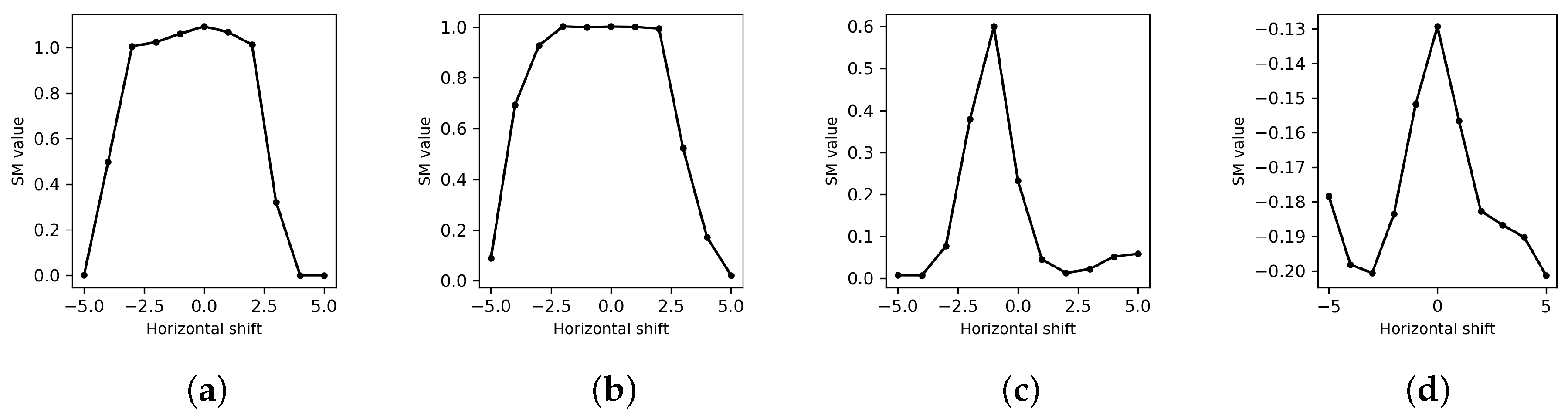
3.2. SM Performance Criteria

An SM takes two image patches—one from a reference image (RI) and the other one from a template image (TI)—as input and outputs a scalar value S M v that measures the similarity between these patches. A binary decision is then made to decide whether these patches are similar or dissimilar by comparing the SM value with a threshold S M t h :
y = 1 , S M v > S M t h , 1 , o t h e r w i s e .
where labels “1” and “−1” correspond to similar and dissimilar patches, respectively. Here, we assume that a higher SM value corresponds to higher similarity. The opposite case, when a lower SM value corresponds to higher similarity, can be reduced to the first one by changing the SM value sign.
Two well-known criteria, namely, the Receiver Operating Characteristic (ROC) and Area Under the Curve (AUC), are generally used to evaluate the quality of such a binary classifier [51].
In image registration, an SM is typically used to localize a PC between registered images [1,2]. A PC can be found as a local maximum of the SM value with respect to a mutual translation vector or a more complex geometrical transform between the compared image patches:
t P C = ( x P C , y P C ) = arg max ( x , y ) Ω ( S M v ( x , y ) )
where t P C = ( x P C , y P C ) is the coordinates of the putative correspondence, and Ω is a search zone within which the true correspondence is expected to be found. For example, a correspondence between images can be found by calculating the NCC absolute value in a sliding scanning window manner and finding the local maximum of the obtained correlation map.
SM values are calculated on a regular grid with unit pixel spacing by gradually shifting RP with respect to TP. Subpixel accuracy can be reached by approximating the output S M v in the maximum neighborhood ( x P C , y P C ) typically by a quadratic function and finding the maximum of the approximation function:
θ ^ = arg max θ ( Δ x = 1 Δ x = 1 ( Δ y = 1 Δ y = 1 ( S M v ( x P C + Δ x , y P C + Δ y ) ( θ 1 Δ x 2 + θ 2 Δ x Δ y + θ 3 Δ y 2 + θ 4 Δ x + θ 5 Δ y + θ 6 ) ) ) )
t ^ P C = t P C 2 θ 1 θ 2 θ 2 2 θ 3 1 θ 4 θ 5
where the second term in (4) is the coordinate of the maximum of the approximating second-order polynomial.
The localization accuracy is characterized by its bias Δ t and its standard deviation (SD) σ t with respect to the components of the translation vector. We will also use the robust SD σ t . M A D calculated as 1.48 · M A D , where M A D is Median Absolute Deviation [52]. Notice, that a smaller σ t or σ t . M A D value corresponds to a better localization accuracy.

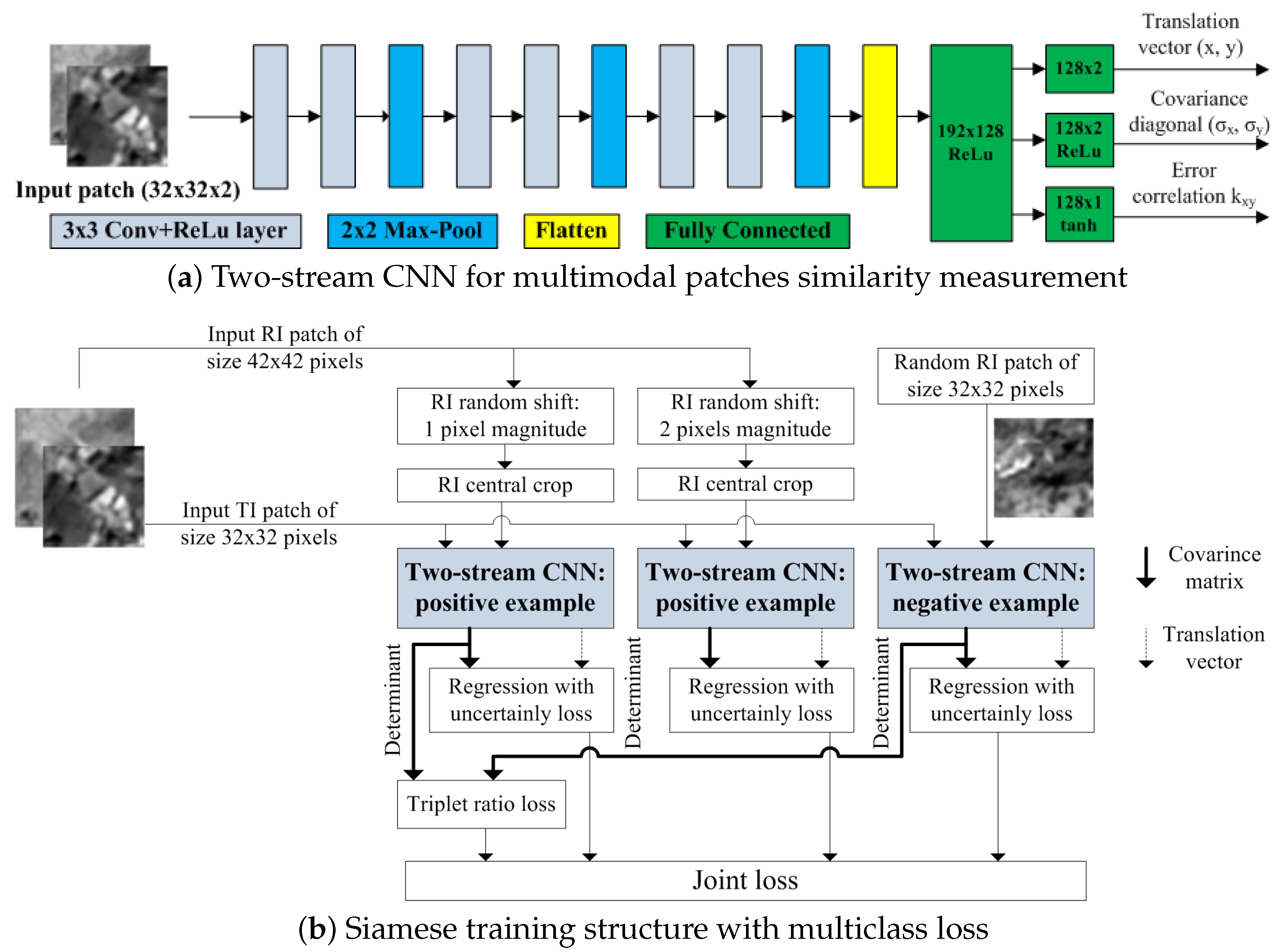
3.3. Patch Matching as Deep Regression with Uncertainty

For an accurate localization, an SM is required to discriminate between not only similar and dissimilar patch pairs, but also slightly shifted versions of similar patches. To better illustrate this idea, let us analyze the approximation approach of the SM value more in detail. For a PC with coordinates ( x P C , y P C ) , the SM value takes a maximum value at ( x P C , y P C ) and decreases in its neighborhood of width Δ m a x pixels: S M v ( x P C , y P C ) > S M v ( x P C + Δ x , y P C + Δ y ) , | Δ x | < Δ m a x , | Δ y | < Δ m a x . Therefore, in the local neighborhood, an SM value can be factorized into two terms as S M v ( x P C , y P C ) g ( Δ x , Δ y ) , where g ( Δ x , Δ y ) 1 , g ( 0 , 0 ) = 1 . The first term S M v ( x P C , y P C ) is responsible for similarity discrimination and is insensitive to spatial misalignment within a local neighborhood of the true correspondence. In turn, the second term g ( Δ x , Δ y ) is sensitive only to spatial misalignment of the compared patches. Loss functions leading to step-like SM profile do not consider the g ( Δ x , Δ y ) term during training and focus on S M v ( x P C , y P C ) only. Loss function leading to smooth SM profile estimate SM value without factorizing it into S M v ( x P C , y P C ) from g ( Δ x , Δ y ) .
Let us represent S M v · g ( Δ x , Δ y ) as a two-dimensional normal distribution 1 2 π | C | e x p ( 0.5 · ( Δ x , Δ y ) · C 1 · ( Δ x , Δ y ) T ) , where C is the translation error covariation matrix and | · | denotes matrix determinant. From this point of view, g ( Δ x , Δ y ) = e x p ( 0.5 · ( Δ x , Δ y ) · C 1 · ( Δ x , Δ y ) T ) characterizes the deviation ellipse of patches localization error, and 1 2 π | C | serves as a similarity measure value.
We propose to formulate similarity measuring as a regression problem with uncertainty. Patch matching CNN estimates the translation vector value t = ( Δ x , Δ y ) and the uncertainty of this estimate in the form of a translation vector estimation error covariance matrix C = σ x 2 σ x σ y k x y σ x σ y k x y σ y 2 , where σ x and σ y are SDs of horizontal and vertical errors in estimating the components of the translation vector, respectively, and k x y denotes the correlation coefficient between these components. As an SM value, we propose to use S M v = S M d e t = | C | = σ x σ y 1 k x y 2 . With this formulation, patch localization and patch discrimination become unified.
Our CNN is trained with the following loss function,
L ( θ , Δ x 0 , Δ y 0 ) = ( Δ x Δ x 0 , Δ y Δ y 0 ) · C 1 · ( Δ x Δ x 0 , Δ y Δ y 0 ) T + l n ( | C | ) = [ ( Δ x Δ x 0 ) 2 σ y 2 + ( Δ y Δ y 0 ) 2 σ x 2 2 ( Δ x Δ x 0 ) ( Δ y Δ y 0 ) σ x σ y k x y 2 ] σ x 2 σ y 2 ( 1 k x y 2 ) + 2 l n ( σ x ) + 2 l n ( σ y ) + l n ( 1 k x y 2 ) = 1 1 k x y 2 ( Δ x Δ x 0 ) 2 σ x 2 + ( Δ y Δ y 0 ) 2 σ y 2 2 k x y 2 ( Δ x Δ x 0 ) ( Δ y Δ y 0 ) σ x σ y + 2 l n ( σ x ) + 2 l n ( σ y ) + l n ( 1 k x y 2 )
where θ = ( Δ x , Δ y , σ x , σ y , k x y ) is parameter vector predicted by the DLSM, ( Δ x 0 , Δ y 0 ) denotes ground truth shift between RP and TP.
The last three terms force the determinant | C | of the covariance matrix of the translation vector estimation error to decrease, thus reducing the uncertainty of estimates. The first term requires the translation estimation error to agree with the predicted covariance matrix. The loss function (5) corresponds to the maximization of the likelihood function for a two-dimensional normal distribution. It can be seen as a two-dimensional version of the loss function for learning regression with uncertainty utilized in [53,54].

3.4. Siamese ConvNet Structure and Training Process Settings

The base structure of the two-stream CNN for measuring multimodal patches similarity is shown in Figure 3a. It consists of three groups of convolutional and pooling layers followed by two fully-connected layers. We selected the input patch size of 32 by 32 pixels. It was noted in [27] that a larger patch size does not provide performance improvement. Both RP and TP are normalized to zero mean and unity variance. Feature vector size for the first block of convolutional layers is N f e a t u r e s = 48 and increases twofold for each following block (96 and 192, respectively). Image size after the first, second, and third pooling layers is 15 × 15 × 48, 6 × 6 × 96, and 2 × 2 × 192, respectively. Feature vector size after the flattening layer is therefore equal to 768. CNN outputs two elements of translation vector ( Δ x , Δ y ) and three elements describing covariation matrix estimate ( σ x , σ y , and k x y ). To enforce the usual properties of covariation matrix elements, the following constraints should be satisfied; σ x > 0 , σ y > 0 and | k x y | < 1 . Consequently, ReLu activation is applied to σ x , σ y , and tanh to k x y .
The structure of two-stream CNN was optimized with respect to two parameters: N f e a t u r e s and the kernel size of the first convolutional layer for extracting features. We found that value N f e a t u r e s above 48 does not impact patch matching accuracy but increases inference time. We thus selected N f e a t u r e s = 48 . Changing kernel size from (3, 3) to (5, 5) does not have an effect on the CNN performance. Therefore, it was set to its minimum value (3, 3).
For the DLSM training, we use positive and negative examples of patch pairs. A positive example represents a truly corresponding multimodal patch pair randomly shifted in the interval from a to a pixels in both dimensions. The value of a defines a PC neighborhood where DLSM is able to detect the PC position. A negative example represents a randomly selected RP/TP pair. For negative examples, ground truth translation vector has no meaning and loss (5) cannot be calculated. Moreover, a negative example should not affect DLSM branch for predicting the translation vector. To process positive and negative examples in a uniform manner, we assume that for negative examples PC prediction errors are random values that do not depend on input data, are uncorrelated, and have the same variance D n e g : E ( ( Δ x Δ x 0 ) 2 ) = E ( ( Δ y Δ y 0 ) 2 ) = D n e g and E ( ( Δ x Δ x 0 ) ( Δ y Δ y 0 ) ) = 0 . Averaging loss (5) over Δ x Δ x 0 and Δ y Δ y 0 yields mean loss value as
L m e a n ( θ ) = 1 1 k x y 2 D n e g σ x 2 + D n e g σ y 2 + 2 l n ( σ x ) + 2 l n ( σ y ) + l n ( 1 k x y 2 )
For a negative example, the DLSM output minimizing mean value of loss (6) can be directly calculated: k x y = 0 , σ x 2 = σ y 2 = D n e g . Therefore, for negative examples, the SM value is forced towards the positive constant D n e g . On the contrary, for positive examples, the SM value is expected to decrease towards zero. For training, we set a = 1.5 2.5 pixels and D n e g = 7 p i x e l s 2 .
For the DLSM training, we decided, similar to triplet losses, to consider simultaneously several patch pairs within a Siamese training architecture as shown in Figure 3b. It comprises three branches. For all branches, the same TP is used. For the first two branches, random positive examples are generated by randomly shifting RP, with a = 1.5 for the first branch and a = 2.5 for the second branch. For the last branch, a negative example is generated. The DLSM is trained with joint loss comprising uncertainty with regression and triplet ratio losses:
l o s s j o i n t ( θ 1 , θ 2 , θ 3 , Δ x 01 , Δ y 01 , Δ x 02 , Δ y 02 ) = w ( Δ x 01 , Δ y 01 ) · L ( θ 1 , Δ x 01 , Δ y 01 ) +     w ( Δ x 02 , Δ y 02 ) · L ( θ 2 , Δ x 02 , Δ y 02 ) + L m e a n ( θ 3 ) + c p o s 2 + ( c n e g 1 ) 2 ,
where ( Δ x 0 i , Δ y 0 i ) is the ground truth translation vector for the ith branch, i = 1 3 , w ( Δ x , Δ y ) = 1 0.1 + Δ x 2 + Δ y 2 is a weighting function emphasizing smaller translation values, and ( c p o s , c n e g ) = s o f t m a x ( | C 1 | , | C 3 | ) is the result of softmax operator applied to the pair of positive SM value for the first branch and negative SM value. The joint loss (7) combines the proposed loss (5) for each branch and triplet ratio loss for two pairs of positive and negative examples. By combining two different losses, we seek to ensure that CNN learns with the goal to both discriminate multimodal patches and correctly estimate translation between them.
The main difference of DLSM lies in extended number of outputs (translation vector and covariance matrix elements instead of just one SM value) and usage of joint loss function. Applied to one patch pair, the DLSM has the same computational complexity as CNNs with other losses: on NVIDIA GeForce GTX 960M GPU inference time is ~0.5 ms (2000 pairs per second). DLSM does not depend on a particular two-stream CNN structure: each two-stream CNN suitable for hidge, triplet, or other existing losses can be transformed to DLSM.

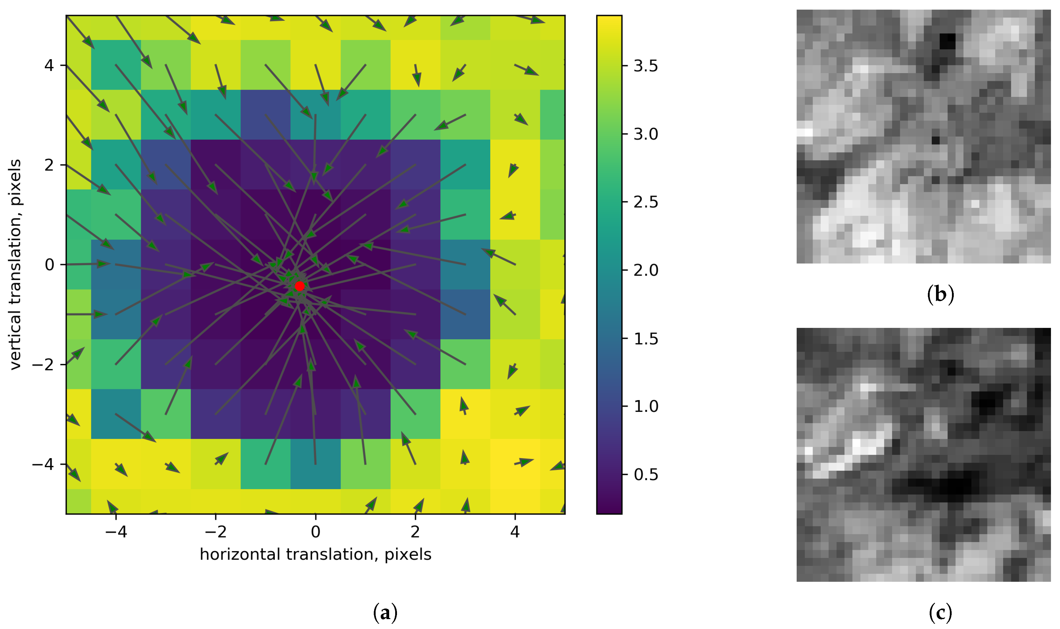
3.5. Patch Pair Alignment with Subpixel Accuracy

Apart from the similarity value, DLSM predicts translation vector between the compared patches. Similar to other SMs, DLSM can be applied to a spatial neighborhood of the given patch pair by shifting TP relative to RP by an integer number of pixels ( u , v ) . For each ( u , v ) , DLSM predicts a slightly different position of the true correspondence (Figure 4 shows an example of ( Δ x , Δ y ) field). Having these multiple measurements, different strategies for the true correspondence localization are possible with DLSM. Let us discuss them in order of increased accuracy established experimentally.
The first strategy is to detect the minimum value of S M d e t with coordinates ( u m i n , v m i n ) and estimate the true correspondence as ( u m i n + Δ x ( u m i n , v m i n ) , v m i n + Δ y ( u m i n , v m i n ) ) .
By design, translation vectors predicted by the DLSM are reliable only in a small neighborhood of the true translation of about two-three pixels in radius. Taking this into account, the second strategy is to repeat the first one two times: localize S M d e t global minimum, obtain the true correspondence position predicted by DLSM, and use the DLSM output at the refined position as the second and final refinement.
Both strategies were found to have similar localization accuracy comparable to that obtained with triplet losses. Their main drawback is that information from neighboring DLSM outputs is not used. Therefore, the third strategy is to localize the true correspondence as a consensus between DLSM predictions in the 3 by 3 neighborhood. For this, the translation vector values are averaged by a box filter with 3 pixels width. The smoothed translation vector ( Δ x . a v g , Δ y . a v g ) is close to zero for those patch pairs where DLSM prediction for neighboring pairs (shifted by −1, 0, or 1 pixel) points to this position. The integer value of the position of the true correspondence is localized as the minimum value of S M d e t · Δ x . a v g 2 + Δ y . a v g 2 + C , where C is a constant experimentally set to 0.5 pixels. Subpixel coordinates are obtained by applying the corresponding subpixel shift ( Δ x . a v g , Δ y . a v g ) .
The fourth strategy extends the previous one even further and takes into account the distribution ellipse of each DLSM prediction:
( Δ ^ x , Δ ^ y ) = arg max ( x , y ) ( u = 2 2 v = 2 2 e x p ( 0.5 · L ( θ ( u , v ) , u x , v y ) ) ) ,
where L ( u x , v y ) is the loglikelihood function (5) value calculated using DLSM parameters for a patch pair shifted by ( u , v ) pixels. We found the latter strategy to have the best localization accuracy. All results in the experimental part of the paper are obtained with this localization strategy.

4. Experimental Part

In this section, both the two-stream CNN-based SMs trained with different loss functions (referred to as DSM, Deep SM) and Siamese CNN-based DLSM are compared to five existing multimodal SMs: (1) an SM which includes two terms, the Mutual Information and a gradient term, which highlights the large gradients with orientations in both modalities (GMI, Gradient with Mutual Information) [55]; (2) SIFT-OCT [15]; (3) MIND [16]; (4) HOPC [13]; and (5) L2-Net descriptor CNN [27]. The proposed loss function is compared to hinge, L 2 , binary cross-entropy (bce), triplet ratio (tr), triplet margin (tm), and multiclass losses. For all variants, we use only single scale input leaving experiments with central-surround input [18] for future work.

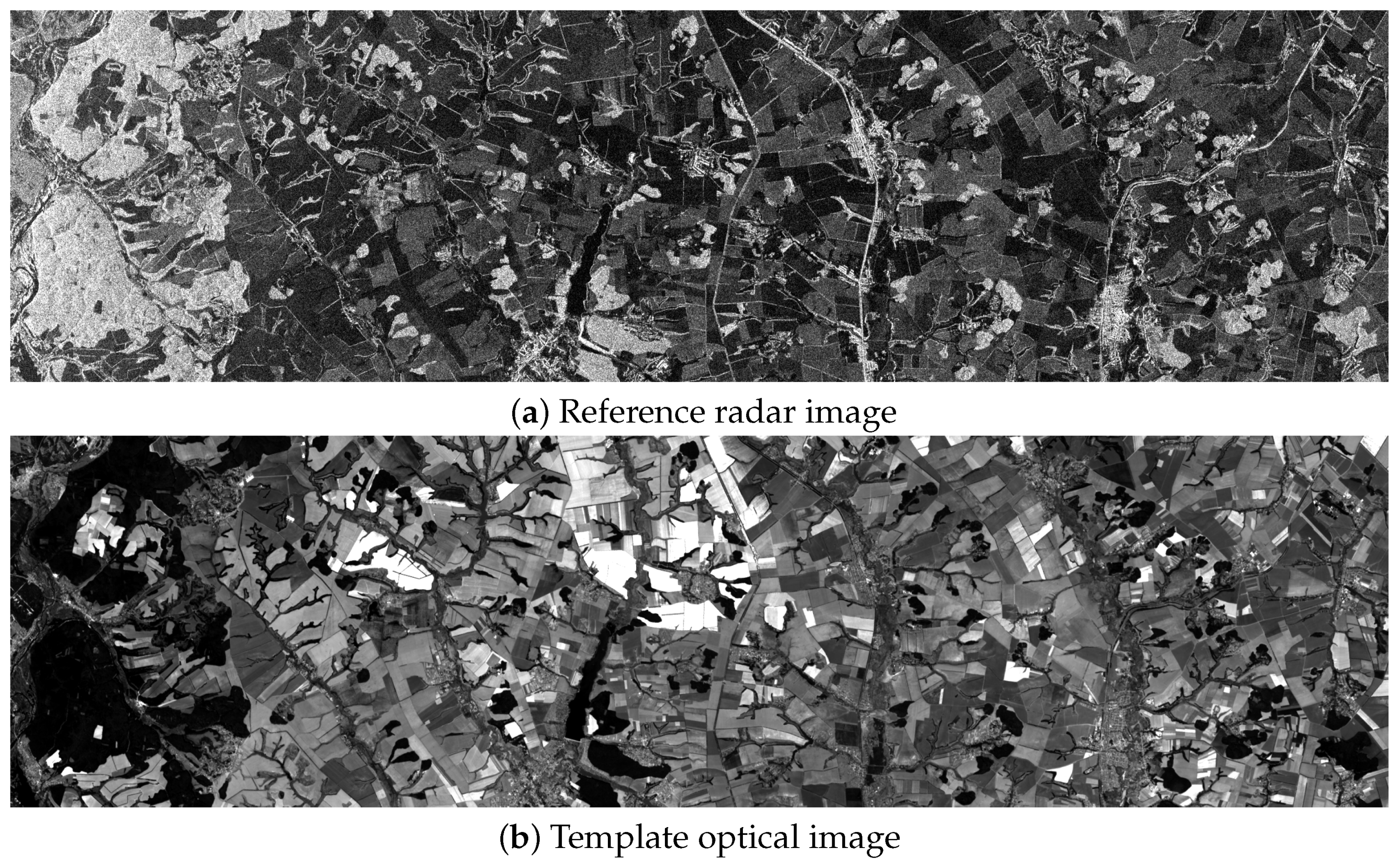
4.1. Multimodal Image Dataset

For training all patch matching CNNs considered in this study, 18 pairs of multimodal images were collected covering visible-to-infrared, optical-to-radar, optical-to-DEM, and radar-to-DEM cases. We use the term “optical” for both visual and infrared modalities. In the following, we group all these cases as the general case. Data from optical modality come from Sentinel 2, Landsat 8 and Hyperion platforms, radar modality from SIR-C and Sentinel 1 platforms, DEM from ASTER Global DEM 2, and ALOS World 30m global DEMs. Each image pair was registered in advance using the previously developed RAE registration method [1]. One example of optical-radar pair is shown in Figure 5.
In total, an amount of 2,700,000 32 × 32 patch pairs was collected from the above mentioned registration cases in the following proportions: 75% for visible-to-infrared, 9% for optical-to-radar, 8% for optical-to-DEM, and 8% for radar-to-DEM. These pairs were randomly split between training (75%) and validation (25%) sets. The proposed CNNs are trained with Adam optimizer [56], initial learning rate 2 · 10 4 and decay 10 5 . Training takes 800 epochs, with each epoch comprising 5000 steps (mini-batches). Batch size is set to 32. The parameters of all existing hand-crafted SMs are chosen according to the recommendations given in their respective papers.
Test data are collected from another set of 16 registered multimodal pairs covering the same registration cases. From this extra set of pairs, 100,000 patch pairs (50% similar and 50% dissimilar) were uniformly collected among the considered registration cases.

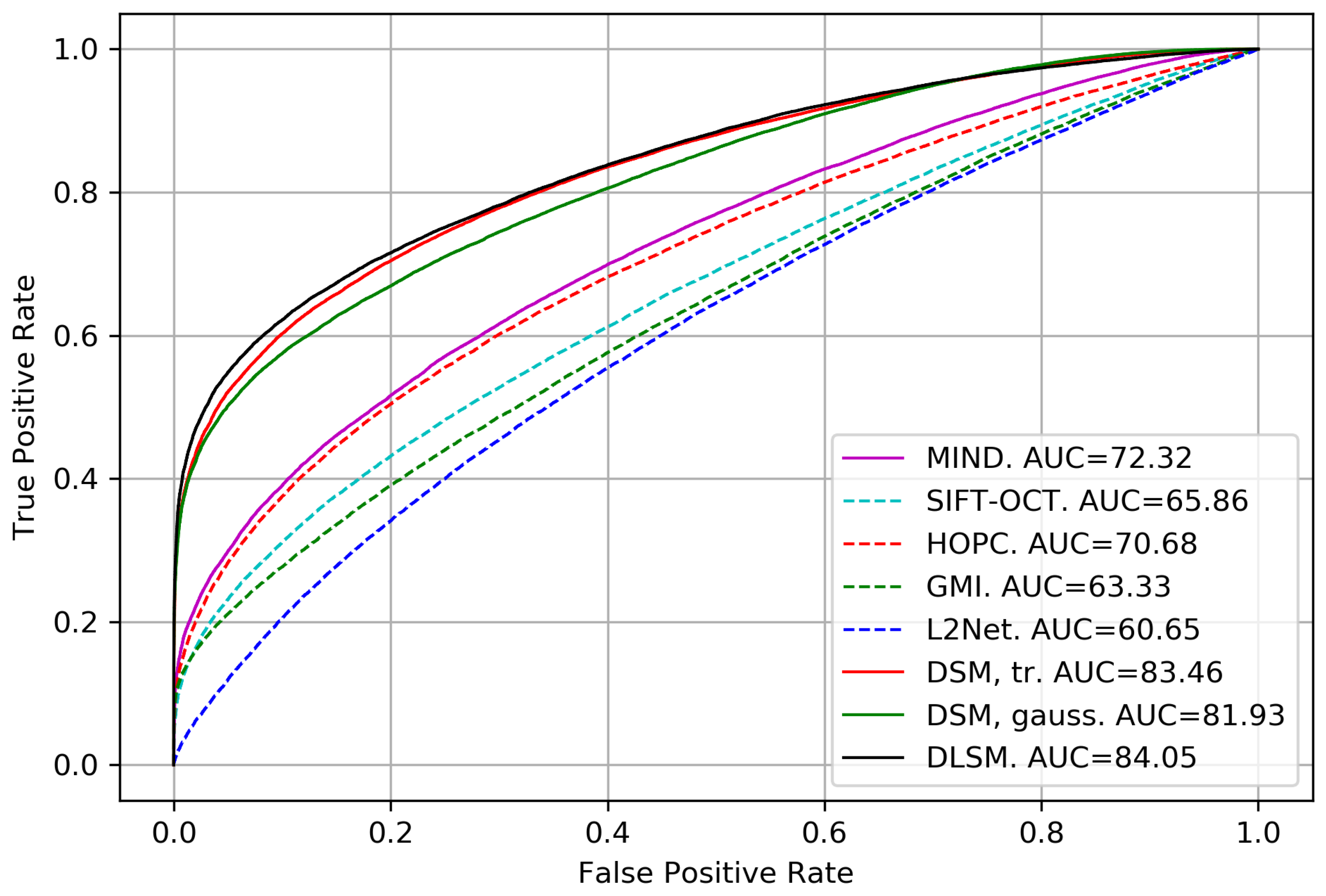
4.2. Discriminative Power Analysis

For the general case, the ROC curves of the SMs selected for comparison are illustrated in Figure 6. ROC curves for the DLSM and DSM trained with the six different losses are close to each other. To avoid figure cluttering, only ROC for DLSM and DSM with the triplet ratio loss are shown. Numerical results for all SMs in comparison and each registration case are given in Table 1.
Among the considered hand-crafted SMs, the MIND has the highest AUC in the general case (72.32%). It also shows the best performance in optical-to-DEM and visible-to-infrared cases. However, in optical-to-radar and radar-to-DEM cases, SIFT-OCT achieves the best performance among hand-crafted SMs. L2-Net performs poorly in multimodal case and has low AUC in all cases. The proposed DLSM shows the best performance among the compared SMs, with AUC higher by 0.5% than the second highest result by the triplet ratio loss. The DLSM provides significant advantage over considered hand-crafted SMs in the general case (gain: ~11.7%) and each particular case (the gain is ~11.8% in optical-to-DEM case, 5% in visible-to-infrared case, 13% in optical-to-radar case, and 17.2% in radar-to-DEM case). Apart from the general case, the DLSM has the highest AUC in optical-to-radar, and radar-to-DEM cases. However, in the optical-to-DEM case, the best AUC is obtained with the triplet ratio loss, and in the optical-to-optical case, by the multiclass loss.

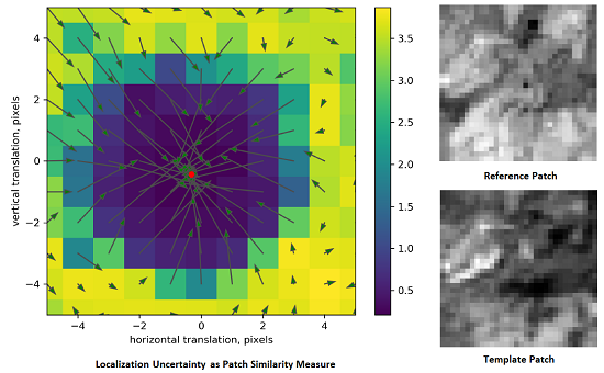
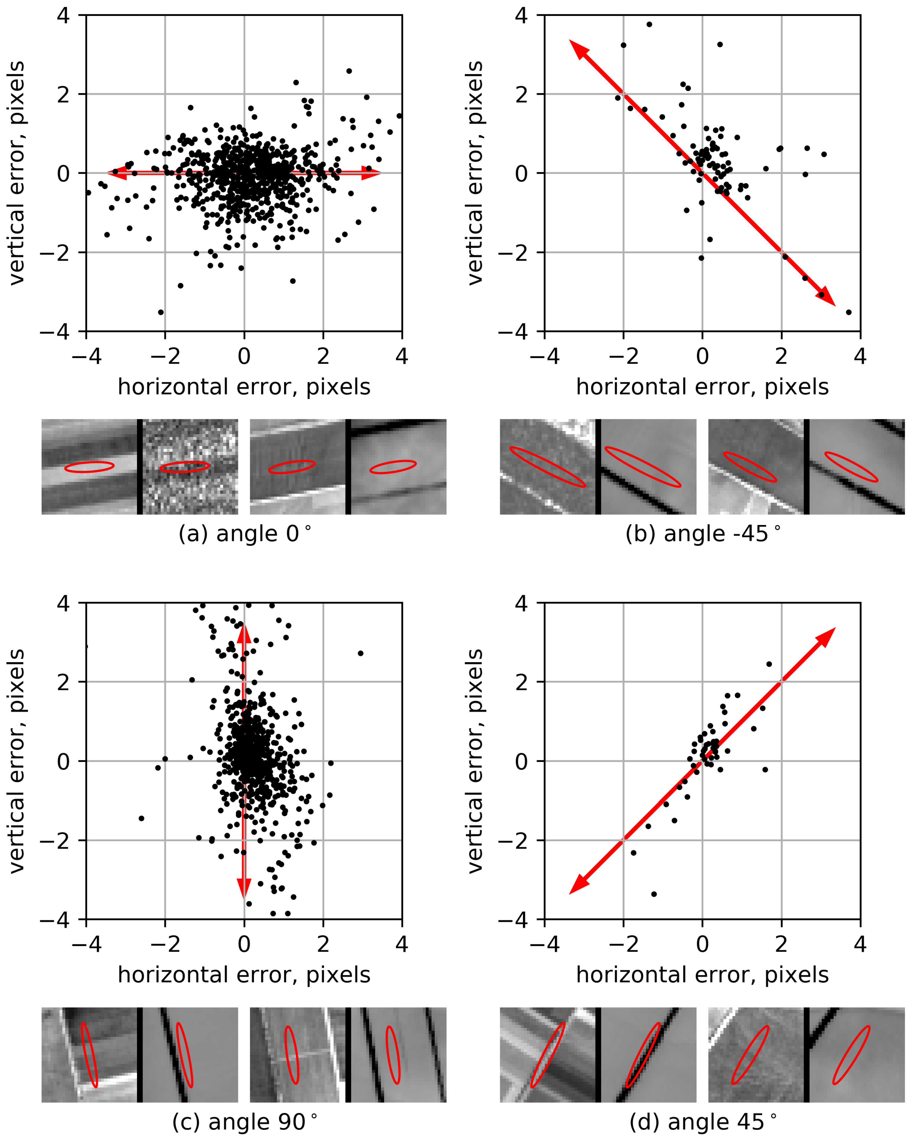
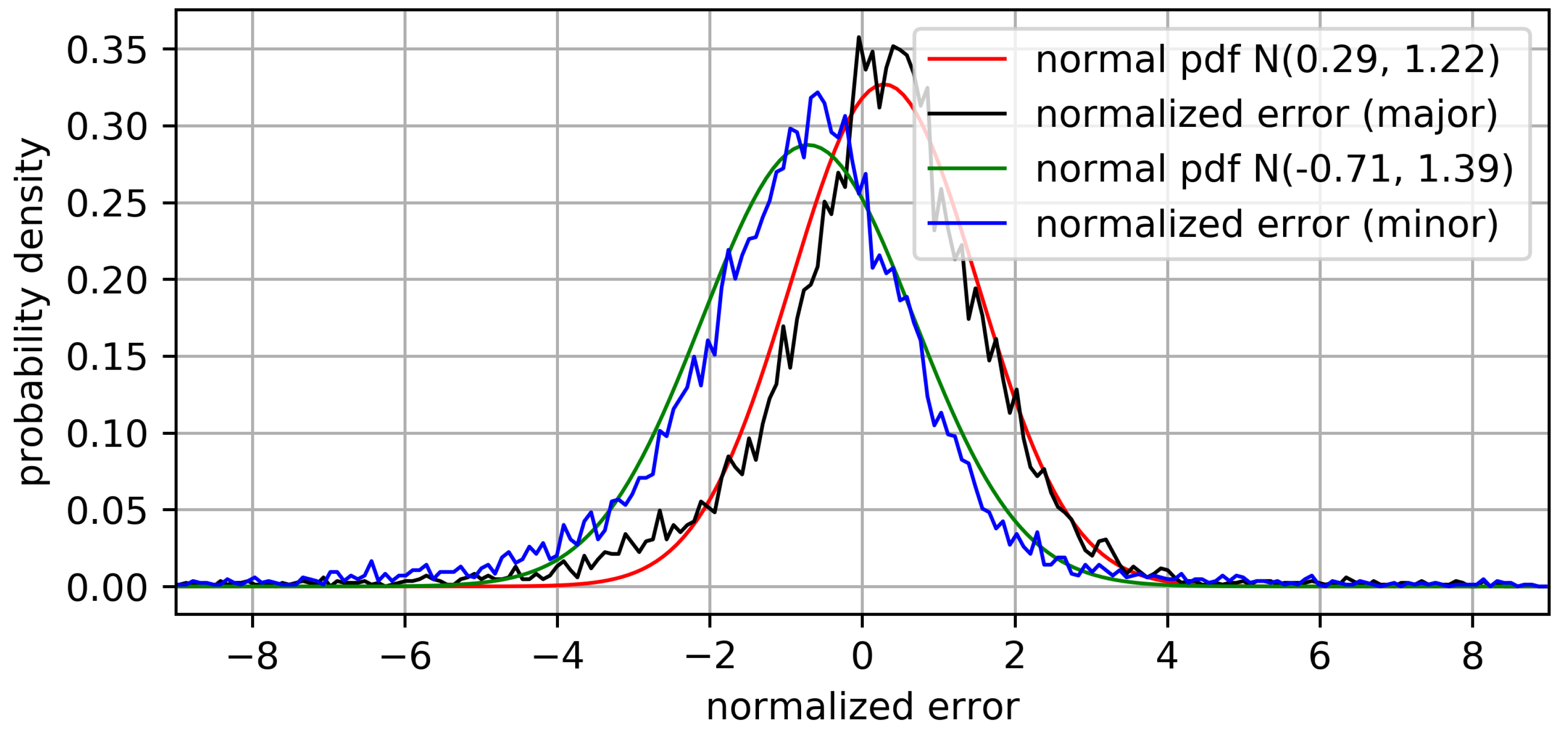
4.3. Patch Matching Uncertainty Analysis

Unlike the majority of prior hand-crafted and learning-based SMs, the proposed DLSM has the ability to predict the distribution of the estimated translation vector between the compared patches. To the best of our knowledge, the only SM with this ability is the logLR (log-likelihood ratio) published by the authors in [12]. However, the logLR can only be applied to isotropic textures, it has a lower discriminative power than that of the MIND and impractically high computational complexity for patch size 32 by 32 pixel. Therefore, we decided not to include it in the comparison.
For each patch pair, the DLSM estimates the covariance matrix C of the translation estimation error. Let us define eigenvalues of C as λ m a x and λ m i n , where λ m a x > λ m i n . The eigenvector corresponding to λ m a x is defined as v m a x = ( c o s ( α c o v ) , s i n ( α c o v ) ) , where 90 < α c o v 90 . The values λ m a x and λ m i n characterize the semi-axis of the estimation error distribution ellipse, the angle α c o v characterizes its orientation, and the ratio r λ = λ m a x / λ m i n 1 characterizes its elongation.
Large values of the r λ ratio indicate that the pair of matched patches has a dominant direction, for example, representing an anisotropic texture. Let us analyze what the patches that lead to high predicted values of r λ by the DLSM look like. We selected patches with λ m a x < 1 pixels and r λ > 3 . These patches are collected into four groups according to the value of α c o v : (1) 15 < α c o v < 15 ; (2) 60 < α c o v < 30 ; (3) 75 < α c o v < 90 or 90 < α c o v < 75 ; (4) 30 < α c o v < 60 . For each group, Figure 7 shows the translation estimation error scatterplot and displays two pairs of patches with the highest ratio r λ . The estimate of the translation error distribution ellipse obtained by DLSM is overlaid on the corresponding patch.
From Figure 7, it is seen that the DLSM correctly detects the patches with correlated translation error components: the error for patches grouped according to the value of α c o v has a distribution with a pronounced orientation aligned with α c o v . Patches with the highest r λ have strongly anisotropic linear oriented structure. Interestingly, the number of patches for the two cases α c o v = ± 45 are significantly lower than for the cases α c o v = 0 , 90 . This effect could be related to the content of the test images. Another possibility is that the distribution ellipse of the estimation errors by DLSM may be biased.
The analysis above is essentially qualitative. To quantitatively characterize the DLSM translation estimation error ϵ = ( Δ x ^ , Δ x ^ ) ( Δ x 0 , Δ y 0 ) , let us normalize the translation vector error as ϵ n o r m = L 1 · ϵ , where C = L L T is the Cholesky decomposition of the covariance matrix. Two particular elements of ϵ n o r m , denoted as ϵ n o r m . m a j o r and ϵ n o r m . m i n o r , correspond to the errors along semi-major and semi-minor axes of the distribution ellipse, respectively. If the estimated covariance matrix C is correct, the normalized error should posses the following properties; ϵ n o r m . m a j o r and ϵ n o r m . m i n o r should follow a standard normal distribution N ( 0 , 1 ) and be uncorrelated.
The experimental distributions of ϵ n o r m . m a j o r and ϵ n o r m . m i n o r are shown in Figure 8 in comparison to the normal distribution. The shape of both pdfs is close to normal, but the parameters differ from standard ones. Both ϵ n o r m . m a j o r and ϵ n o r m . m i n o r are slightly biased and have an SD of ~1.3 instead of 1. This deviation can be, at least partially, explained by a not perfect registration of the train and test data. Let us assume, that registration error of the test data is normal with SD σ t e s t and bias b t e s t . For a translation error with SD σ t r u e , the normalized error will have SD 1 + ( σ t e s t / σ t r u e ) 2 and bias b t e s t / σ t r u e . For the considered set of test images, we checked that the observed bias of the normalized translation error can be caused by b t e s t = 0.1 0.15 and that of SD by σ t e s t = 0.15 pixels. This level of registration error is quite normal for multimodal images registration. Given the characteristics of the test data, the DLSM prediction of the covariance matrix of translation vector estimation errors for multimodal patches is very accurate.

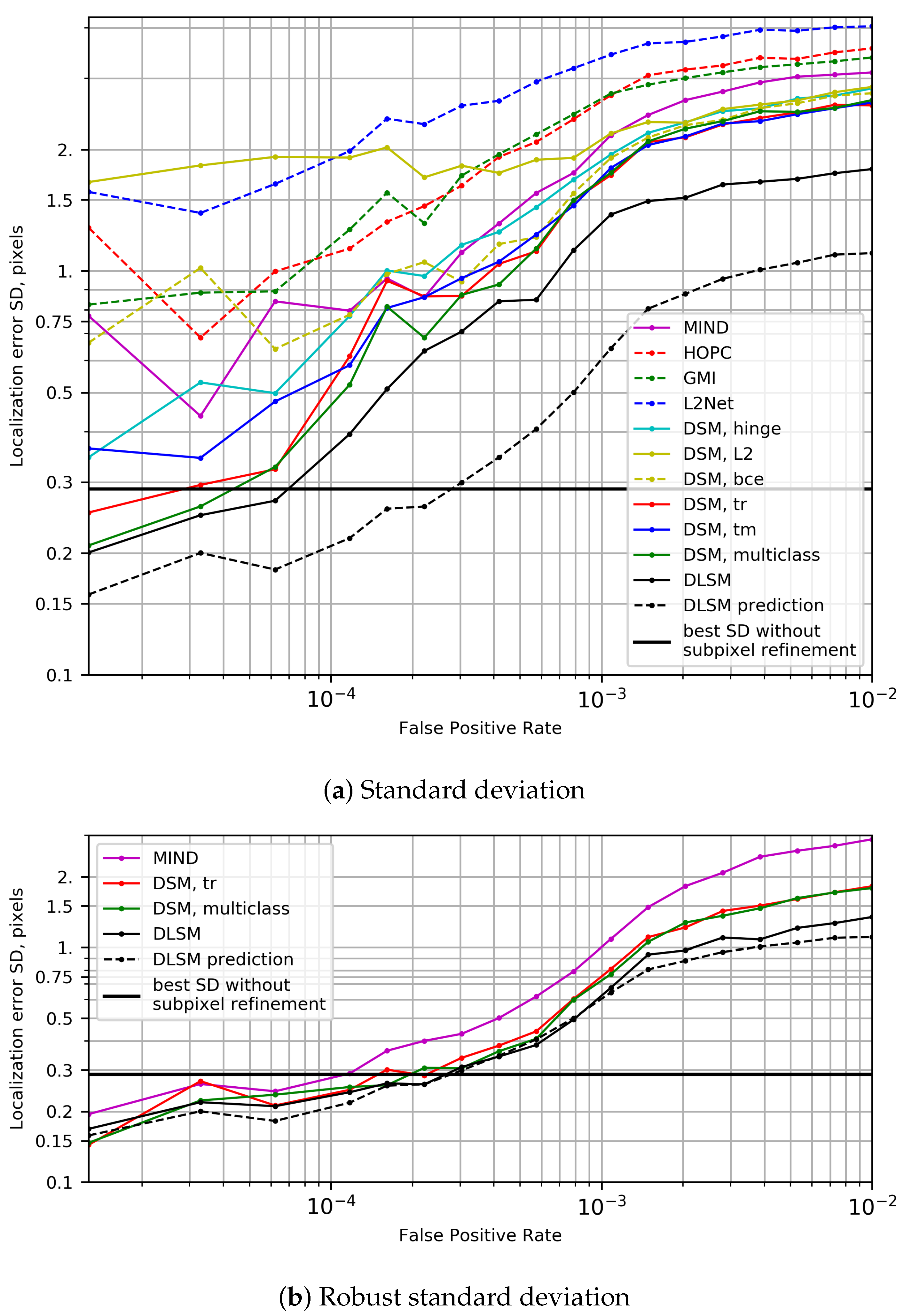
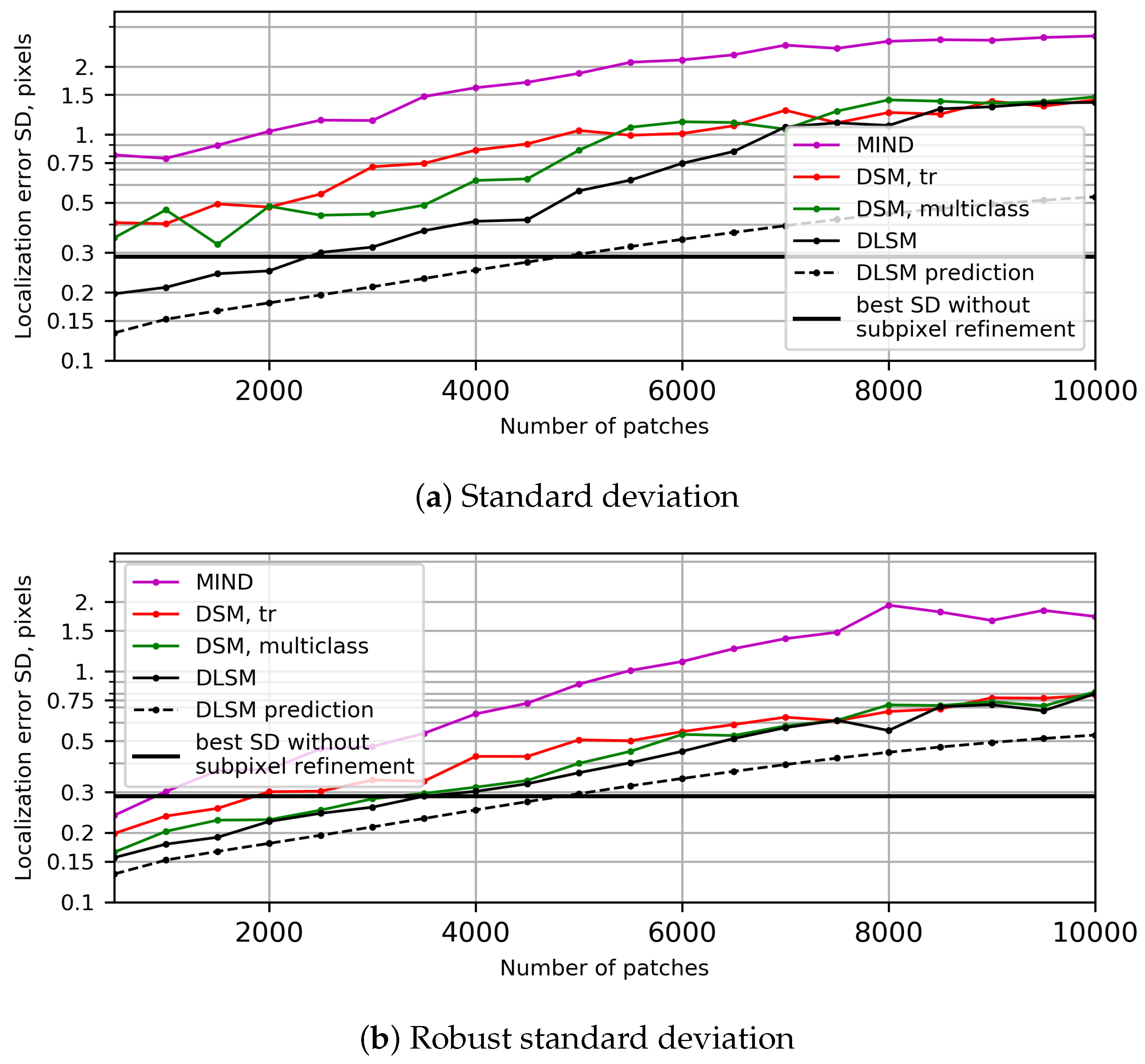
4.4. Localization Accuracy Analysis

In the analysis of the localization accuracy of SMs, we pursue two goals: comparing the localization accuracy for the same set of patches for different SMs and studying the localization accuracy dependence on the SM value. For the first experiment, we selected the hand-crafted SM with the highest AUC—MIND—as a reference SM and ordered all patches in order of decreasing similarity established by MIND. For each value of MIND descriptor, the corresponding False Positive Rate (FPR) value is calculated. The FPR value ranges from 10 6 to 10 2 and is split into 30 intervals using a logarithmic scale. All patches with MIND value falling into the same FPR interval are grouped together. The translation vector error SD and robust SD are calculated for each interval and for each SM.
To calculate the translation error for each patch, a random subpixel shift in the range −3...3 pixels is first applied in both directions with respect to TP getting a modified TP. This shift represents the ground truth value. For each SM, its value is calculated by translating the modified TP in the interval from −5 to 5 pixels in horizontal and vertical directions. The coordinates of the SM main extrema are found and then refined to subpixel values according to (4). For the proposed DLSM, the translation vector is estimated according to the fourth strategy described in Section 4.3. The translation estimation error is calculated as the difference between the estimated and ground truth translation vectors.
The SD and robust SD of the localization error as a function of the MIND FPR is shown in Figure 9a,b, respectively, for the compared set of SMs. If the localization of a PC is implemented with integer precision, the best reachable error SD corresponds to the SD of a uniform distribution in the interval [ 0.5 , 0.5 ] pixels equal to 0.2887. This value is marked for reference as the black thick line in Figure 9a,b. Below we will refer to it as subpixel accuracy level.
For all SMs, the SD of the localization accuracy increases when the FPR decreases, that is, for more similar SMs. This is a natural observation, as very similar patches produce a delta-function-like SM shape. SIFT-OCT has the worst localization accuracy exceeding 1.5 pixels even for the most similar patches. The MIND SM is characterized by the best localization accuracy among the hand-crafted SMs. However, MIND accuracy never reaches subpixel accuracy. This is caused by outlying estimates. The SD calculated in a robust manner (Figure 9b) exceeds the subpixel accuracy level for FPR less than 2 · 10 4 .
Note that among the considered learning-based SMs, four have a step-like SM profile: DSM with hinge, L 2 , binary cross-entropy losses, and the proposed DLSM. Three SMs have the smooth profile: DSM with triplet ratio, triplet margin, and multiclass losses. DSMs with the stepwise profile have localization accuracy worse than MIND; DSM with the smooth profile has a better localization accuracy than MIND. DLSM possesses advantages of both groups: the stepwise SM profile (see Figure 4) and the best localization accuracy over the compared SMs. In average, the DLSM improves SD by about 1.86 times as compared to MIND, by 1.28 as compared to the multiclass loss, and by 1.36 as compared to the triplet loss. For multiclass and triplet losses, subpixel accuracy for FPR is ~ 5 · 10 5 and for DLSM for FPR is ~ 7 · 10 5 . For robust SD, DLSM has also the highest accuracy but the gain is less visible: about 1.63 times as compared to MIND, by 1.15 as compared to the multiclass loss, and by 1.20 as compared to the triplet loss.
As discussed above, DLSM is able to predict its localization accuracy. This prediction is shown in both Figure 9a,b. For robust SD, predicted accuracy follows closely the measured values. For non-robust SD, measured accuracy is lower due to outliers influence.
In the next experiment, we compare the absolute number of reliable PCs provided by each SM. For this, SMs in comparison are applied to all corresponding test patches (50,000 in total). For each SM, patches are sorted in decreasing order of similarity. The SD and robust SD are calculated for successive groups of 500 patches. For the first 10,000 pairs, the dependencies of (robust) SD on the increasing number of patches are shown in Figure 10 for MIND, triplet ratio loss and DLSM.
In contrast to the previous experiment, both SM discriminative power and localization accuracy are important. According to SD measure, DLSM detects ~2400 patches with subpixel localization accuracy, whereas triplet ratio loss, multiclass loss, and MIND detect none of them. For the first group of 500 patches, DLSM results in SD of 0.195, multiclass loss of 0.35, triplet loss of SD of 0.4 pixels, and MIND-SD of 0.8 pixels. According to the robust SD measure, DLSM detects 3500 patches with subpixel localization accuracy, triplet loss of 1840, multiclass loss of 3090, and MIND of 590 patches. For the first group of 500 patches, DLSM results in an SD of 0.156, multiclass loss of 0.165, triplet loss of SD of 0.2, and MIND-SD of 0.244 pixels. In this case, the DLSM SM value also accurately describes the observed translation vector estimation error of the DLSM.
In practice, multimodal registration requires few, but accurate and reliable matching points [24]. For this, the ability of DLSM to detect and localize high quality correspondences is important.

5. Conclusions

In this paper, we have proposed a new CNN structure for training a multimodal similarity measure that satisfies two properties: a high discriminative power and accurate localization of the compared patches.
Analysis of the existing patch matching CNNs and loss functions commonly used for their training revealed that the accurate localization is not a property explicitly considered. Therefore, subpixel localization accuracy can only be obtained for losses such as triplet ratio, triplet margin, and multi-class cross entropy, and only for a limited number of patches.
We have chosen to consider the discrimination and location of two patches not as different problems but as two sides of the same problem. We assume that a pair of patches are easier to align when they become more similar. Or conversely, uncertainty of a patches’ pair localization can serve as a measure of their similarity. The proposed CNN, called DLSM, solves a regression task with the uncertainty taken into account and predicts the translation vector between two patches as well as the covariance matrix of the prediction error of this translation vector. The determinant of the predicted covariance matrix is a measure of localization uncertainty and we use it as a similarity value. The proposed CNN is trained with a specific joint regression–classification loss.
The experiments performed on 16 multimodal image pairs representing visual-infrared, optical-radar, optical-to-DEM, and radar-to-DEM cases have shown that the DLSM achieves both superior discriminating power and localization accuracy. The DLSM has desired step-like SM profile, but with localization accuracy better than SMs with the smooth SM profile. Thanks to the stepwise profile, a PC between reference and template images can be found by calculating DLSM values on a coarse translation grid. However, unlike hinge, L 2 , and binary cross entropy losses, PC can be accurately localized.
In addition to a high discrimination power and high localization accuracy, another aspect of DLSM is important in practice. Unlike existing SMs, DLSM is able to predict the covariance matrix of the translation vector prediction error. We found that the DLSM correctly predicts the covariance matrix of localization errors for different modalities, isotropic, and anisotropic patches and different noise levels. This property is essential for the selection and proper weighting of putative correspondences in advanced image registration methods.

Author Contributions

M.U. conceived of the paper, designed the experiments, generated the dataset, wrote the source code, performed the experiments, and wrote the paper. B.V. performed the experiments and revised the manuscript. V.L. and K.C. provided detailed advice during the writing process and revised the manuscript. All authors have read and agreed to the published version of the manuscript.

Funding

This research received no external funding.

Conflicts of Interest

The authors declare no conflict of interest.

Abbreviations

The following abbreviations are used in this manuscript:
RSRemote Sensing
SMSimilarity Measure
CNNConvolutional Neural Network
DLSMDeep Localization Similarity Measure
PCPutative Correspondence
DEMDigital Elevation Model
SSDSum of Squared Differences
NCCNormalized Correlation Coefficient
SIFTScale-Invariant Feature Transform
MIMutual Information
HOPCHistogram of Orientated Phase Congruency
MINDModality Independent Neighborhood Descriptor
SNRSignal-to-Noise Ratio
FCFully Connected (layer)
SARSynthetic Aperture Radar
RPReference Patch
TPTemplate Patch
ROCReceiver Operating Characteristic
AUCArea Under the Curve
FPRFalse Positive Rate
SDStandard Deviation
MADMedian Absolute Deviation
DSMDeep Similarity Measure
pdfprobability density function

References

  1. Uss, M.; Vozel, B.; Lukin, V.; Chehdi, K. Multimodal remote sensing images registration with accuracy estimation at local and global scales. IEEE Trans. Geosci. Remote Sens. 2016, 54, 6587–6605. [Google Scholar] [CrossRef] [Green Version]
  2. Ma, J.; Zhao, J.; Tian, J.; Yuille, A.L.; Tu, Z. Robust Point Matching via Vector Field Consensus. IEEE Trans. Image Process. 2014, 23, 1706–1721. [Google Scholar] [CrossRef] [PubMed] [Green Version]
  3. Le Moigne, J.; Netanyahu, N.S.; Eastman, R.D. Image Registration for Remote Sensing; Cambridge University Press: Cambridge, UK, 2011. [Google Scholar]
  4. En, S.; Lechervy, A.; Jurie, F. TS-NET: Combining Modality Specific and Common Features for Multimodal Patch Matching. In Proceedings of the 2018 25th IEEE International Conference on Image Processing (ICIP), Athens, Greece, 7–10 October 2018; pp. 3024–3028. [Google Scholar] [CrossRef] [Green Version]
  5. Aguilera, C.A.; Aguilera, F.J.; Sappa, A.D.; Aguilera, C.; Toledo, R. Learning cross-spectral similarity measures with deep convolutional neural networks. In Proceedings of the IEEE Conference on Computer Vision and Pattern Recognition Workshops, Las Vegas, NV, USA, 26 June–1 July 2016; pp. 1–9. [Google Scholar]
  6. Aguilera, C.A.; Sappa, A.D.; Aguilera, C.; Toledo, R. Cross-Spectral Local Descriptors via Quadruplet Network. Sensors 2017, 17, 873. [Google Scholar] [CrossRef] [PubMed] [Green Version]
  7. Goshtasby, A.; Le Moign, J. Image Registration: Principles, Tools and Methods; Springer: London, UK, 2012. [Google Scholar]
  8. Zitová, B.; Flusser, J. Image registration methods: A survey. Image Vis. Comput. 2003, 21, 977–1000. [Google Scholar] [CrossRef] [Green Version]
  9. Roche, A.; Malandain, G.; Pennec, X.; Ayache, N. The correlation ratio as a new similarity measure for multimodal image registration. In Medical Image Computing and Computer-Assisted Interventation—MICCAI’98; Springer: Heidelberg, Germany, 1998; pp. 1115–1124. [Google Scholar]
  10. Foroosh, H.; Zerubia, J.B.; Berthod, M. Extension of phase correlation to subpixel registration. IEEE Trans. Image Process. 2002, 11, 188–200. [Google Scholar] [CrossRef] [Green Version]
  11. Suri, S.; Reinartz, P. Mutual-Information-Based Registration of TerraSAR-X and Ikonos Imagery in Urban Areas. IEEE Trans. Geosci. Remote Sens. 2010, 48, 939–949. [Google Scholar] [CrossRef]
  12. Uss, M.; Vozel, B.; Lukin, V.; Chehdi, K. Statistical power of intensity- and feature-based similarity measures for registration of multimodal remote sensing images. Proc. SPIE 2016, 10004. [Google Scholar] [CrossRef]
  13. Ye, Y.; Shan, J.; Bruzzone, L.; Shen, L. Robust Registration of Multimodal Remote Sensing Images Based on Structural Similarity. IEEE Trans. Geosci. Remote Sens. 2017, 55, 2941–2958. [Google Scholar] [CrossRef]
  14. Lowe, D. Distinctive Image Features from Scale-Invariant Keypoints. Int. J. Comput. Vis. 2004, 60, 91–110. [Google Scholar] [CrossRef]
  15. Suri, S.; Schwind, P.; Uhl, J.; Reinartz, P. Modifications in the SIFT operator for effective SAR image matching. Int. J. Image Data Fusion 2010, 1, 243–256. [Google Scholar] [CrossRef] [Green Version]
  16. Heinrich, M.P.; Jenkinson, M.; Bhushan, M.; Matin, T.; Gleeson, F.V.; Brady, S.M.; Schnabel, J.A. MIND: Modality independent neighbourhood descriptor for multi-modal deformable registration. Med. Image Anal. 2012, 16, 1423–1435. [Google Scholar] [CrossRef] [PubMed]
  17. Yi, K.M.; Trulls, E.; Lepetit, V.; Fua, P. Lift: Learned invariant feature transform. In European Conference on Computer Vision; Springer: Heidelberg, Germany, 2016; pp. 467–483. [Google Scholar]
  18. Zagoruyko, S.; Komodakis, N. Learning to compare image patches via convolutional neural networks. In Proceedings of the IEEE Conference on Computer Vision and Pattern Recognition, Boston, MA, USA, 7–12 June 2015; pp. 4353–4361. [Google Scholar]
  19. Zeng, A.; Song, S.; Nießner, M.; Fisher, M.; Xiao, J.; Funkhouser, T. 3dmatch: Learning local geometric descriptors from rgb-d reconstructions. In Proceedings of the IEEE Conference on Computer Vision and Pattern Recognition, Honolulu, HI, USA, 21–26 July 2017; pp. 1802–1811. [Google Scholar]
  20. Schonberger, J.L.; Hardmeier, H.; Sattler, T.; Pollefeys, M. Comparative evaluation of hand-crafted and learned local features. In Proceedings of the IEEE Conference on Computer Vision and Pattern Recognition, Honolulu, HI, USA, 21–26 July 2017; pp. 1482–1491. [Google Scholar]
  21. Yang, X.; Kwitt, R.; Styner, M.; Niethammer, M. Quicksilver: Fast predictive image registration—A deep learning approach. NeuroImage 2017, 158, 378–396. [Google Scholar] [CrossRef] [PubMed]
  22. Balakrishnan, G.; Zhao, A.; Sabuncu, M.R.; Guttag, J.; Dalca, A.V. An unsupervised learning model for deformable medical image registration. In Proceedings of the IEEE Conference on Computer Vision and Pattern Recognition, Salt Lake City, UT, USA, 18–22 June 2018; pp. 9252–9260. [Google Scholar]
  23. Altwaijry, H.; Trulls, E.; Hays, J.; Fua, P.; Belongie, S. Learning to Match Aerial Images with Deep Attentive Architectures. In Proceedings of the 2016 IEEE Conference on Computer Vision and Pattern Recognition (CVPR), Las Vegas, NV, USA, 27–30 June 2016; pp. 3539–3547. [Google Scholar] [CrossRef]
  24. Merkle, N.; Luo, W.; Auer, S.; Müller, R.; Urtasun, R. Exploiting Deep Matching and SAR Data for the Geo-Localization Accuracy Improvement of Optical Satellite Images. Remote Sens. 2017, 9, 586. [Google Scholar] [CrossRef] [Green Version]
  25. Uss, M.L.; Vozel, B.; Dushepa, V.A.; Komjak, V.A.; Chehdi, K. A precise lower bound on image subpixel registration accuracy. IEEE Trans. Geosci. Remote Sens. 2013, 52, 3333–3345. [Google Scholar] [CrossRef]
  26. Torr, P.H.S.; Zisserman, A. MLESAC: A New Robust Estimator with Application to Estimating Image Geometry. Comput. Vis. Image Underst. 2000, 78, 138–156. [Google Scholar] [CrossRef] [Green Version]
  27. Tian, Y.; Fan, B.; Wu, F. L2-net: Deep learning of discriminative patch descriptor in euclidean space. In Proceedings of the IEEE Conference on Computer Vision and Pattern Recognition, Honolulu, HI, USA, 21–26 July 2017; pp. 661–669. [Google Scholar]
  28. Han, X.; Leung, T.; Jia, Y.; Sukthankar, R.; Berg, A.C. Matchnet: Unifying feature and metric learning for patch-based matching. In Proceedings of the IEEE Conference on Computer Vision and Pattern Recognition, Boston, MA, USA, 7–12 June 2015; pp. 3279–3286. [Google Scholar]
  29. Žbontar, J.; LeCun, Y. Stereo matching by training a convolutional neural network to compare image patches. J. Mach. Learn. Res. 2016, 17, 2287–2318. [Google Scholar]
  30. Simo-Serra, E.; Trulls, E.; Ferraz, L.; Kokkinos, I.; Fua, P.; Moreno-Noguer, F. Discriminative learning of deep convolutional feature point descriptors. In Proceedings of the IEEE International Conference on Computer Vision, Boston, MA, USA, 7–12 June 2015; pp. 118–126. [Google Scholar]
  31. Hadsell, R.; Chopra, S.; LeCun, Y. Dimensionality reduction by learning an invariant mapping. In Proceedings of the 2006 IEEE Computer Society Conference on Computer Vision and Pattern Recognition (CVPR’06), New York, NY, USA, 17–22 June 2006; Volume 2, pp. 1735–1742. [Google Scholar]
  32. Georgakis, G.; Karanam, S.; Wu, Z.; Ernst, J.; Košecká, J. End-to-end learning of keypoint detector and descriptor for pose invariant 3D matching. In Proceedings of the IEEE Conference on Computer Vision and Pattern Recognition, Salt Lake City, UT, USA, 18–22 June 2018; pp. 1965–1973. [Google Scholar]
  33. Mobahi, H.; Collobert, R.; Weston, J. Deep learning from temporal coherence in video. In Proceedings of the 26th Annual International Conference on Machine Learning; ACM: New York, NY, USA, 2009; pp. 737–744. [Google Scholar]
  34. Balntas, V.; Johns, E.; Tang, L.; Mikolajczyk, K. PN-Net: Conjoined triple deep network for learning local image descriptors. arXiv 2016, arXiv:1601.05030. [Google Scholar]
  35. Choy, C.B.; Gwak, J.; Savarese, S.; Chandraker, M. Universal correspondence network. In Proceedings of the Advances in Neural Information Processing Systems 29: Annual Conference on Neural Information Processing Systems, Barcelona, Spain, 5–10 December 2016; pp. 2414–2422. [Google Scholar]
  36. Deng, H.; Birdal, T.; Ilic, S. Ppfnet: Global context aware local features for robust 3d point matching. In Proceedings of the IEEE Conference on Computer Vision and Pattern Recognition, Salt Lake City, UT, USA, 18–22 June 2018; pp. 195–205. [Google Scholar]
  37. Hoffer, E.; Ailon, N. Deep Metric Learning Using Triplet Network. International Workshop on Similarity-Based Pattern Recognition; Springer International Publishing: Cham, Switzerland, 2015; pp. 84–92. [Google Scholar]
  38. Khoury, M.; Zhou, Q.Y.; Koltun, V. Learning compact geometric features. In Proceedings of the IEEE International Conference on Computer Vision, Venice, Italy, 22–29 October 2017; pp. 153–161. [Google Scholar]
  39. Masci, J.; Migliore, D.; Bronstein, M.M.; Schmidhuber, J. Descriptor learning for omnidirectional image matching. In Registration and Recognition in Images and Videos; Springer: Heidelberg, Germany, 2014; pp. 49–62. [Google Scholar]
  40. Wang, J.; Song, Y.; Leung, T.; Rosenberg, C.; Wang, J.; Philbin, J.; Chen, B.; Wu, Y. Learning fine-grained image similarity with deep ranking. In Proceedings of the IEEE Conference on Computer Vision and Pattern Recognition, Columbus, OH, USA, 23–28 June 2014; pp. 1386–1393. [Google Scholar]
  41. Suárez, P.L.; Sappa, A.D.; Vintimilla, B.X. Cross-spectral image patch similarity using convolutional neural network. In Proceedings of the 2017 IEEE International Workshop of Electronics, Control, Measurement, Signals and their Application to Mechatronics (ECMSM), Donostia-San Sebastian, Spain, 24–26 May 2017; pp. 1–5. [Google Scholar] [CrossRef]
  42. He, H.; Chen, M.; Chen, T.; Li, D. Matching of Remote Sensing Images with Complex Background Variations via Siamese Convolutional Neural Network. Remote Sens. 2018, 10, 355. [Google Scholar] [CrossRef] [Green Version]
  43. Kumar, B.; Carneiro, G.; Reid, I. Learning local image descriptors with deep siamese and triplet convolutional networks by minimising global loss functions. In Proceedings of the IEEE Conference on Computer Vision and Pattern Recognition, Las Vegas, NV, USA, 27–30 June 2016; pp. 5385–5394. [Google Scholar]
  44. Yang, Z.; Dan, T.; Yang, Y. Multi-Temporal Remote Sensing Image Registration Using Deep Convolutional Features. IEEE Access 2018, 6, 38544–38555. [Google Scholar] [CrossRef]
  45. Simonyan, K.; Zisserman, A. Very deep convolutional networks for large-scale image recognition. arXiv 2014, arXiv:1409.1556. [Google Scholar]
  46. Deng, J.; Dong, W.; Socher, R.; Li, L.; Kai, L.; Li, F.F. ImageNet: A large-scale hierarchical image database. In Proceedings of the 2009 IEEE Conference on Computer Vision and Pattern Recognition, Miami, FL, USA, 20–25 June 2009; pp. 248–255. [Google Scholar]
  47. Luo, W.; Schwing, A.G.; Urtasun, R. Efficient deep learning for stereo matching. In Proceedings of the IEEE Conference on Computer Vision and Pattern Recognition, Las Vegas, NV, USA, 26 June– 1 July 2016; pp. 5695–5703. [Google Scholar]
  48. Dosovitskiy, A.; Springenberg, J.T.; Riedmiller, M.; Brox, T. Discriminative unsupervised feature learning with convolutional neural networks. In Proceedings of the Advances in Neural Information Processing Systems 27: Annual Conference on Neural Information Processing Systems, Montreal, QC, Canada, 8–13 December 2014; pp. 766–774. [Google Scholar]
  49. Ye, Y.; Bruzzone, L.; Shan, J.; Bovolo, F.; Zhu, Q. Fast and Robust Matching for Multimodal Remote Sensing Image Registration. IEEE Trans. Geosci. Remote Sens. 2019, 57, 9059–9070. [Google Scholar] [CrossRef] [Green Version]
  50. Goncalves, H.; Corte-Real, L.; Goncalves, J.A. Automatic Image Registration Through Image Segmentation and SIFT. IEEE Trans. Geosci. Remote Sens. 2011, 49, 2589–2600. [Google Scholar] [CrossRef] [Green Version]
  51. Fawcett, T. An introduction to ROC analysis. Pattern Recognit. Lett. 2006, 27, 861–874. [Google Scholar] [CrossRef]
  52. Huber, P.J. Robust Statistics; Springer: Berlin/Heidelberg, Germany, 2011. [Google Scholar]
  53. Gurevich, P.; Stuke, H. Learning uncertainty in regression tasks by deep neural networks. arXiv 2017, arXiv:1707.07287. [Google Scholar]
  54. Kendall, A.; Gal, Y. What uncertainties do we need in bayesian deep learning for computer vision? In Proceedings of the Advances in Neural Information Processing Systems 30: Annual Conference on Neural Information Processing Systems, Long Beach, CA, USA, 4–9 December 2017; pp. 5574–5584. [Google Scholar]
  55. Pluim, J.P.W.; Maintz, J.B.A.; Viergever, M.A. Image registration by maximization of combined mutual information and gradient information. IEEE Trans. Med. Imag. 2000, 19, 809–814. [Google Scholar] [CrossRef] [PubMed]
  56. Kingma, D.P.; Ba, J. Adam: A method for stochastic optimization. arXiv 2014, arXiv:1412.6980. [Google Scholar]
Figure 1. Convolutional neural network (CNN) architectures for measuring similarity between image patches.
Remotesensing 12 00703 g001
Figure 2. Shape of SMs as a function of horizontal translation between a pair of similar patches: (a) hinge loss, (b) L 2 loss, (c) multiclass loss, and (d) MIND SM. For patch matching CNN with hinge and L 2 losses, unity SM value means high similarity; zero SM value means no similarity. For patch matching CNN with multiclass loss, higher SM values correspond to higher similarity. Patch matching CNN structure is described in Section 3.4. For MIND, lower SM values mean higher similarity. Inverse MIND value is shown for consistency. Profiles are obtained for a pair of similar visual and infrared patches from Landsat 8 and Sentinel 2 sensors. SMs values are calculated by mutually shifting RP and TP by an integer number of pixels in horizontal direction in interval −5...5 pixels.
Remotesensing 12 00703 g002
Figure 3. The proposed Siamese CNN structure.
Remotesensing 12 00703 g003
Figure 4. Deep Localization Similarity Measure (DLSM) prediction (a) of translation value between a patch pair: (b) reference patch and (c) template patch. The colorbar corresponds to the SM value. Each predicted translation vector is shown as an arrow starting in the input translation between patches and ended in predicted correspondence position. The true correspondence is marked by the red dot.
Remotesensing 12 00703 g004
Figure 5. Example of one training image pair. (a) reference radar image acquired by Sentinel-1 and (b) template optical image acquired by Landsat-8.
Remotesensing 12 00703 g005
Figure 6. Receiver Operating Characteristic (ROC) curves for the proposed DLSM and existing SMs for the general registration case.
Remotesensing 12 00703 g006
Figure 7. DLSM translation prediction errors grouped together. Each panel corresponds to a specific deviation ellipse orientation (the major axis is marked as double headed error): (a) α c o v = 0 , (b) α c o v = 45 , (c) α c o v = 90 , and (d) α c o v = 45 .
Remotesensing 12 00703 g007
Figure 8. Experimental probability function of normalized translation vector estimation error by DLSM.
Remotesensing 12 00703 g008
Figure 9. Localization error SD using Modality Independent Neighborhood Descriptor (MIND) as reference vs. SM quantile.
Remotesensing 12 00703 g009
Figure 10. Localization error vs. The number of patches.
Remotesensing 12 00703 g010
Table 1. Area Under the Curve (AUC) in % for SMs in comparison for general and particular registration cases. The best AUC in each registration case is marked in bold.
MethodGeneralOptical-DEMOptical-OpticalOptical-RadarRadar-DEM
GMI63.3360.8372.1664.3960.19
SIFT-OCT65.8658.9765.7873.5168.21
HOPC70.6767.4378.4170.1667.26
MIND72.3268.6185.1570.3164.51
L2-Net60.6561.8571.2155.5055.41
DSM, hinge80.6676.7487.7779.3276.20
DSM, L 2 80.2576.3088.9977.2975.98
DSM, binary cross-entropy81.1476.3689.8878.6076.68
DSM, triplet ratio loss83.4681.1990.1880.4481.14
DSM, triplet margin loss82.8879.0690.5780.1780.28
DSM, multiclass loss81.9375.0392.4979.4478.32
DLSM84.0779.9690.2183.1681.73

