Uncertainty Analysis for Topographic Correction of Hyperspectral Remote Sensing Images

Abstract

Quantitative uncertainty analysis is generally taken as an indispensable step in the calibration of a remote sensor. A full uncertainty propagation chain has not been established to set up the metrological traceability for surface reflectance inversed from remotely sensed images. As a step toward this goal, we proposed an uncertainty analysis method for the two typical semi-empirical topographic correction models, i.e., C and Minnaert, according to the ‘Guide to the Expression of Uncertainty in Measurement (GUM)’. We studied the data link and analyzed the uncertainty propagation chain from the digital elevation model (DEM) and at-sensor radiance data to the topographic corrected radiance. We obtained spectral uncertainty characteristics of the topographic corrected radiance as well as its uncertainty components associated with all of the input quantities by using a set of Earth Observation-1 (EO-1) Hyperion data acquired over a rugged soil surface partly covered with snow. Firstly, the relative uncertainty of cover types with lower radiance values was larger for both C and Minnaert corrections. Secondly, the trend of at-sensor radiance contributed to a spectral feature, where the uncertainty of the topographic corrected radiance was poor in bands below 1400 nm. Thirdly, the uncertainty components associated with at-sensor radiance, slope, and aspect dominated the total combined uncertainty of corrected radiance. It was meaningful to reduce the uncertainties of at-sensor radiance, slope, and aspect for reducing the uncertainty of corrected radiance and improving the data quality. We also gave some suggestions to reduce the uncertainty of slope and aspect data.

1. Introduction

The development of imaging spectroscopy leads optical remote sensing to hyperspectral remote sensing. The special three-dimensional structure of hyperspectral remote sensing data provides more properties for land surface. At the same time, the higher spectral resolution makes the spectral response finer and provides more effective means for recognizing the targets.

The Guide to the Expression of Uncertainty in Measurement (GUM) [1] is a widely used methodology to evaluate uncertainties in measurements. The Quality Assurance Framework for Earth Observation (QA4EO) [2] was written and endorsed by the Committee on Earth Observation Satellites (CEOS) based on GUM, stating the key principle that “Data and derived products shall have associated with them a fully traceable indicator of their quality.” It encourages the quantification of uncertainties and indicates the importance of quality indicator and traceability. In reality, “different spectra for the same substance” and “the same spectrum for different substances” in the application of hyperspectral remotely sensed data also show the uncertainty of the spectral characteristics. Therefore, in hyperspectral quantitative analysis and application, measurement needs to be traceable to ensure good data quality.

From 2015, the Horizon 2020 project “FIDelity and Uncertainty in Climate data from Earth Observation” (FIDUCEO) [3] conducted (i) a thorough metrological uncertainty analysis for each instrument and (ii) a recalibration using enhanced input data, such as reconstructed spectral response function (SRF). The project is also based on GUM and focuses on uncertainties of climate data records.

For pre-processing in earth observation, the uncertainty research is limited. Pre-processing is a necessary process for remote sensing data including spectral calibration, radiometric calibration, geometric correction, topographic correction, and atmospheric correction. Subsequent research on metrological traceability and uncertainty analysis only concentrated on parts of the entire data pre-processing until now.

For spectral calibration and radiometric calibration, uncertainty analysis is generally taken as an important and indispensable step [4,5,6,7,8]. Woolliams et al. wrote a course text which provides an introduction to uncertainty analysis for earth observation instrument calibration and suggests a step-by-step methodical approach [4]. Chrien et al. verified the laboratory calibration of Airborne Visible Infrared Imaging Spectrometer (AVIRIS) determined through an in-flight calibration experiment and reported the quantitative result that the spectral calibration of AVIRIS agrees with the in-flight data to within 2 nm. The absolute radiometric calibration is consistent with the in-flight verification to 10% over the spectral range [5]. Bachmann et al. conducted uncertainty analysis for radiometric calibration and spectral calibration using the Monte Carlo approach and analyzed the influence on data products (two vegetation indices). The study got the qualitative conclusion that the uncertainty in the Environmental Mapping and Analysis Program (EnMAP) L2A product is wavelength-dependent and also spatially variable over the scene [6].

For atmospheric correction of remote sensing data over a flat terrain, a few studies on uncertainty analysis were conducted [9,10]. Honkavaara et al. studied the uncertainties propagated via image processing and proposed a method of calculating the uncertainty of surface reflectance using the Empirical Line Method (ELM). The surface reflectance and its standard deviation were obtained, but correlations were not considered in their research [9]. Jia et al. also studied the uncertainty of reflectance propagated by ELM and put their effort into the uncertainty estimation of linear regression. They considered correlations in their study [10].

For remote sensing data over rugged terrains, topographic correction is the step that follows radiometric calibration. A rugged terrain leads to radiance variation between pixels which have different topographic features, but the same surface cover type, so that the spectral features of the object could be seriously interfered and accurate classification is hardly achievable. Therefore, topographic correction and its uncertainty analysis are also necessary.

The existing topographic correction models can be divided into three types: empirical model, physical model, and semi-empirical model. The empirical models are based on an empirical relationship between the radiance received by the sensor and the cosine of the effective incident angle. The Tillet Regression Model [11] attempts to remove the influence of terrain on direct solar irradiance by linear regression between the at-sensor radiance and the cosine of the incident angle. Its error in the mountainous area is large, because in a rugged area, the radiance over a flat terrain needed in this method is hard to acquire, and it was obtained only by calculating the mean value of same objects [12]. The b correction model [13] and the Variable Empirical Coefficient Algorithm (VECA) model [14] are both based on this empirical relationship, but they make some improvements. The b correction method has two selective equations to choose the better one in correction and the VECA model has a variable coefficient to correct the radiance. Both of them do not have overcorrection and the VECA is easier and more operable. Another widely used empirical model is the normalized topographic correction model (also called two-stage normalization, 2SN) [15], which obtains correction coefficient by shaded and sunlit slope data and carries out a second correction. More two-stage correction methods [16,17] were proposed after this.

Physical models, based on the Lambertian assumption, include the cosine correction [11], Sun–canopy–sensor (SCS) correction [18], and radiative transfer (RT) models. Cosine correction introduces a term associated with Sun zenith, based on the geometric relationship of "Sun–surface–sensor". The SCS correction considers vegetation gravitropism for mountainous forest, based on the geometric relationship of "Sun–canopy–sensor". These two physical models only consider direct solar irradiance onto the rugged terrain, and often bring obvious overcorrection. The Proy model [19], one of the RT models, divides the total radiation received by a pixel on the slope into three parts: direct solar radiation, sky scattering, and surrounding terrain reflection radiation. It takes sky scattering and surrounding terrain reflection radiation into account, especially focusing on the latter. Some scholars made a more elaborate division for the radiative transfer process and optimized the RT models after this [20].

Compared to the empirical models which often have a large error and the physical models which involve many parameters and complex calculation, the semi-empirical models balance the accuracy and complexity to some degree. To improve the correction effect, some scholars successively introduced empirical parameters into pure physical functions and formed semi-empirical models, including C correction [11], SCS+C correction [21], Minnaert correction [22], and Minnaert+SCS correction [23]. The C correction and SCS+C correction models introduce the empirical parameter c for Lambertian surface, while Minnaert correction and Minnaert+SCS correction introduce the empirical constant k for non-Lambertian surface.

Currently, there is no relevant research on uncertainty analysis for topographic correction. The existing validations of the corrected results mainly rely on visual contrast and statistical comparison. They do not account for uncertainty in either inputs or output. It is important to note that the correction uncertainty varies depending on input quantities as well as empirical parameters.

Within this study, we selected two classical semi-empirical topographic correction models, i.e., C correction and Minnaert correction, to propose an uncertainty analysis method for a typical semi-empirical topographic correction process. We established the uncertainty propagation model, according to the GUM [1] issued by the Joint Committee for Guides in Metrology, by summing up the data link of the correction process. We stressed on the uncertainty propagation analysis, more in general cases than for specific surface types, because topographic correction is just one of the pre-processing steps to get better remotely sensed applications (i.e., classification). We conducted an exemplar experiment by using a set of Earth Observation-1 (EO-1) Hyperion data acquired over a mountainous area in China, with surface type of soil partly covered with snow. The metrological traceability of the C correction and Minnaert correction processes was preliminarily realized.

2. Methods

2.1. Data Link of Topographic Correction

2.1.1. Core Formulas

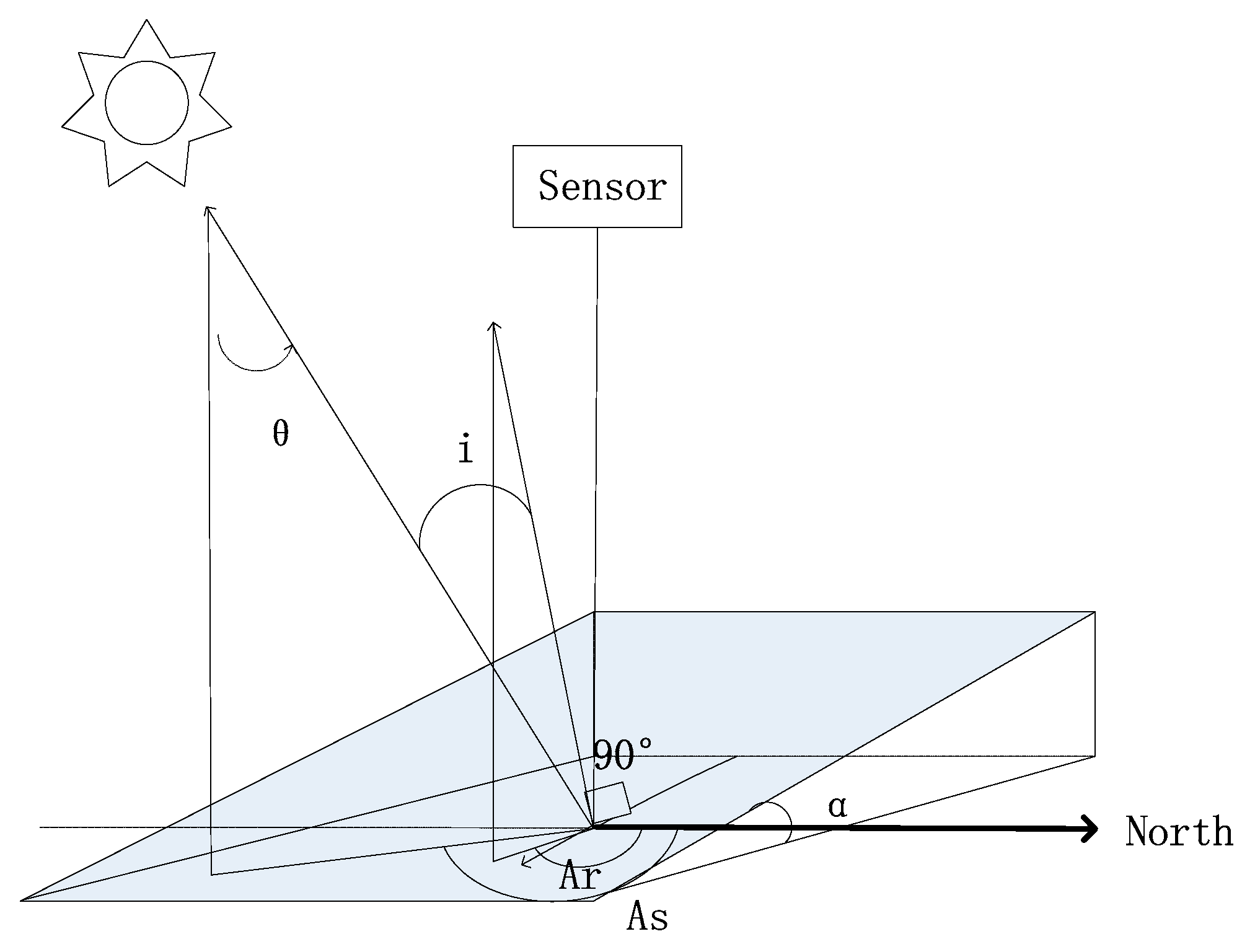
The two typical semi-empirical topographic correction models selected in this study were based on the cosine correction model and aided by the digital elevation model (DEM) data. According to the geometric relationship of Sun–surface–sensor" as shown in Figure 1, the cosine correction model [11] can be expressed as:

$$L_H=L_T\frac{\mathit{cos}\theta }{\mathit{cos}i},$$

(1)

where $L_H$ is the corrected radiance observed from horizontal surface (simply called corrected radiance), $L_T$ is the radiance before correction observed from the inclined face (generally the at-sensor radiance), i is the solar incident angle, and $\theta$ is the solar zenith angle.

C correction is based on uniform and isotropic Lambertian surface. The linear relationship between the radiance of the incline and the cosine of incident angle was used for empirical fitting, and factor c was introduced for adjustment. The core correction equation [11] is:

$$L_H=L_T\frac{\mathit{cos}\theta +c}{\mathit{cos}i+c} ,$$

(2)

where c is the C correction empirical parameter.

Minnaert correction is based on non-Lambertian surface. Minnaert constant k, which describes the bidirectional reflectance distribution function (BRDF) of objects, was introduced into the expression. The correction equation [22] is:

$$L_H=L_T\frac{\mathit{cos}e}{{\mathit{cos}}^k e {\mathit{cos}}^{k}i} ,$$

(3)

where e is the solar exitance angle and k is the Minnaert constant. It is assumed that the sensor is over the target, so the solar exitance angle is equal to the slope angle. Equation (4) is calculated as:

$$L_H=L_T\frac{\mathit{cos}\alpha }{{\mathit{cos}}^k \alpha {\mathit{cos}}^{k}i} .$$

(4)

2.1.2. Data Link

In actual topographic correction, L_T is obtained directly from the at-sensor radiance of hyperspectral images. The other inputs are obtained by further calculation.

The cosine of the solar incident angle is calculated by Equation (5) [11], which expresses the triangular relation in Figure 1:

$$\mathit{cos}i=\mathit{cos}\theta \mathit{cos}\alpha +\mathit{sin}\theta \mathit{sin}\alpha \mathit{cos}(A_s-A_r),$$

(5)

where $\alpha$ is the slope of the surface, A_r is the aspect of the surface, and A_s is the solar azimuth angle. The solar illumination parameters, which include the solar zenith angle and the solar azimuth angle, are important parameters in radiative transfer. They describe the direction and orientation of solar ray onto the target. The topographic parameters, which include the slope angle and the aspect angle, are calculated based on DEM data according to Equations (6) and (7) [24]:

$$\alpha =\mathit{arctan}(\sqrt{f_x^2+f_y^2}),$$

(6)

$$A_r=270+\mathit{arctan}[\frac{f_y}{f_x}\left]-90\times \right[\frac{f_x}{\left|f_x\right|}],$$

(7)

where f_x and f_y are the gradients in the North–South and East–West directions, respectively. They are calculated by the third-order finite difference weighted by reciprocal of squared distance (3FDWRSD) [25].

Using the linear relationship between the at-sensor radiance and the cosine of the solar incident angle, the regression equation is established as Equation (8) [11]:

$$L_T=l+m\cdot \mathit{cos}i,$$

(8)

where l and m denote the intercept and the slope of the line, respectively. Then empirical parameter c is the ratio of the intercept to the slope:

$$c=l/m.$$

(9)

Equation (3) is transformed into:

$$L_{T}cos\alpha =L_H{\mathit{cos}}^k i co{s}^k\alpha ,$$

(10)

and then taking the logarithm of both sides of the equation as Equation (11) [22]:

$$\mathit{log}(L_T\mathit{cos}\alpha )=\mathit{log}{L}_H+k\cdot \mathit{log}(\mathit{cos}i\mathit{cos}\alpha ).$$

(11)

Minnaert constant k is obtained by a linear regression with $x=\mathit{log}(\mathit{cos}i\mathit{cos}\alpha )$ regarded as the independent variable and $y=\mathit{log}(L_T\mathit{cos}\alpha )$ regarded as the dependent variable. Each band of hyperspectral data should be fitted independently.

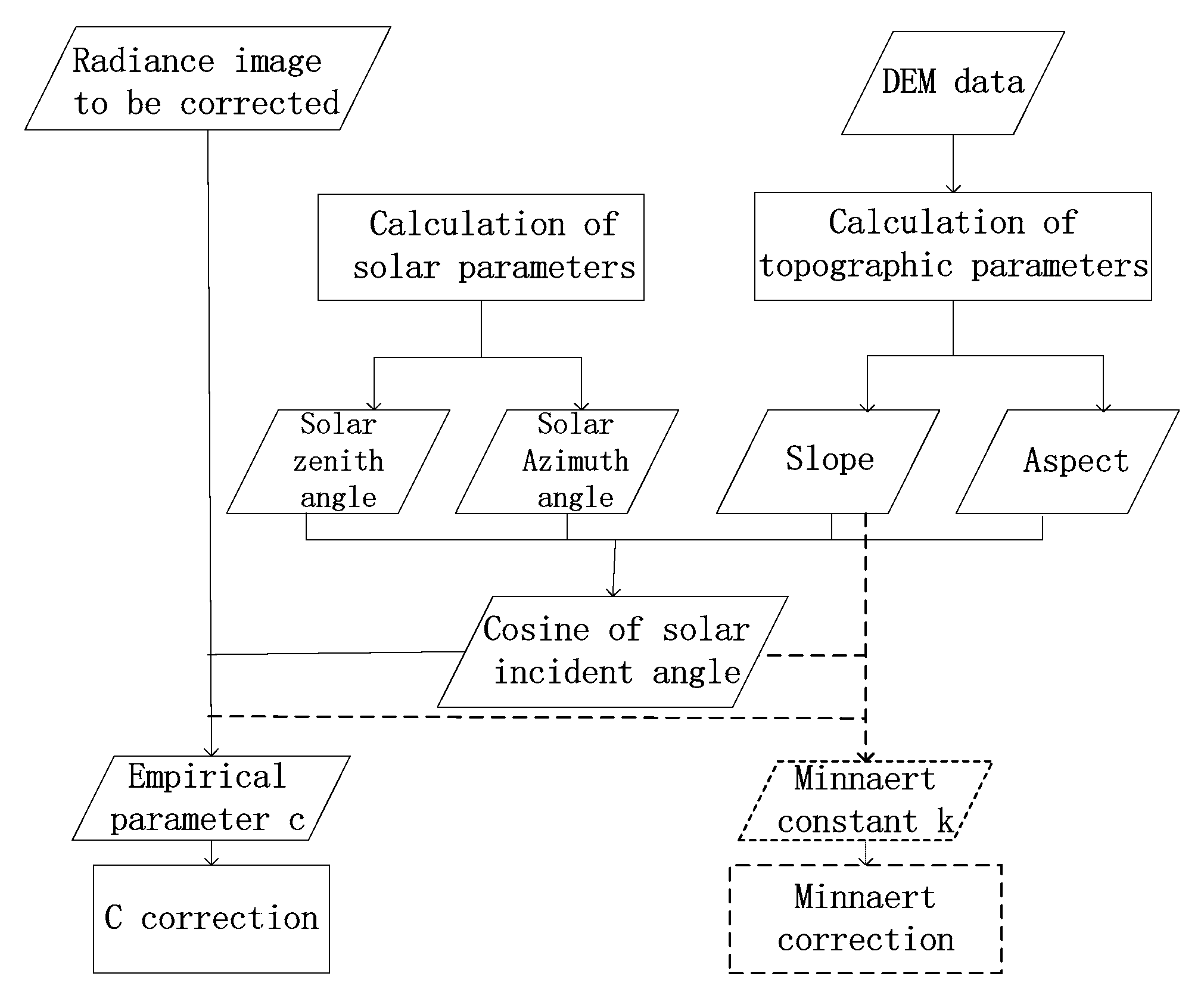
The outputs of C and Minnaert corrections are traced back to DEM data and the at-sensor radiance according to the core correction formulas. The data link, which describes the transmission from the inputs to the output via calculation models, is shown in Figure 2.

2.2. Uncertainty Propagation

2.2.1. General Concepts

According to GUM and the International Vocabulary of Metrology (VIM) [26], the process of uncertainty estimation, based on the propagation law of uncertainty and the mathematical model, is as follows:

1. Defining the measurement equation

In most cases, a measurand $Y$ is not measured directly, but is determined from N other quantities $X_1,X_2,\dots ,X_N$ through the function:

$$Y=f\left(X_1,X_2,\dots ,X_N\right),$$

(12)

$\mathrm{where} x_i$ and $y_i$ are the estimates of the measurands $X_i$ and $Y_i,$ respectively, then the measurement equation can be written as:

$$y=f\left(x_1,x_2,\dots ,x_N\right).$$

(13)

2. Considering the sources of uncertainty

Each term in the measurement equation has associated uncertainties and should be listed. Each uncertainty should be traced back to uncertainty sources. Then the traceability chain is established.

3. Calculating the uncertainty of each input quantities

The standard uncertainty (simply called uncertainty) of each input quantity, denoted as $u\left(x_i\right)$, should be calculated on the basis of type A or type B evaluation of standard uncertainty.

4. Determining combined standard uncertainty

There are two cases. When some of the input quantities are correlated (the estimated variables in measurement, not the physical quantities assumed to be invariants), the equation for the combined variance associated with the result of a measurement is:

$$u_c^2\left(y\right)={\displaystyle \sum }_{i=1}^N{[\frac{\partial f}{\partial x_i}]}^2{u}^2\left(x_i\right)+2{\displaystyle \sum }_{i=1}^{N-1}{\displaystyle \sum }_{j=i+1}^N\frac{\partial f}{\partial x_i}\frac{\partial f}{\partial x_j}u\left(x_i,x_j\right).$$

(14)

$\mathrm{where} u\left(x_i,x_j\right)$ is the estimated covariance associated with $x_i$ and $x_j$, which are interdependent. Samples of $x_i$ and $x_j$ are used to calculate the covariance between the two as:

$$u\left(x_i,x_j\right)=\mathit{cov}(x_i,x_j)=E\left\{\left[x_i-E\left(x_i\right)\right]\left[x_j-E\left(x_j\right)\right]\right\},$$

(15)

where E denotes the expectation of the variables [1]. When all of the input quantities are independent, $u\left(x_i,x_j\right)=0$.

The square root of the combined covariance is the combined standard uncertainty (simply called combined uncertainty).

5. Determining expanded uncertainty

The expanded uncertainty $U$ is obtained by multiplying the combined standard uncertainty by a coverage factor $k_p$, considering the level of confidence p:

$$U=k_p{u}_c\left(y\right).$$

(16)

The result of a measurement is then expressed as $Y=y\pm U$, which means that the best estimate of the measurand $Y$ is $y$, and $y-U$ to $y+U$ is an interval that may be expected to encompass a large fraction of the distribution of values that could reasonably be attributed to $Y$.

6. Reporting uncertainty

The measurement results are expressed as $y\pm U$ using the estimated value $y$, expanded uncertainty $U$, and the level of confidence p.

2.2.2. Uncertainty Sources

The core correction formulas of C and Minnaert corrections are the measurement equations. The corrected radiance $L_H$ is considered as the measurand. In C correction, $L_T$, $\theta$, i, and c are considered as the input quantities. In Minnaert correction, $L_T$, $\alpha$, i, and k are considered as the input quantities.

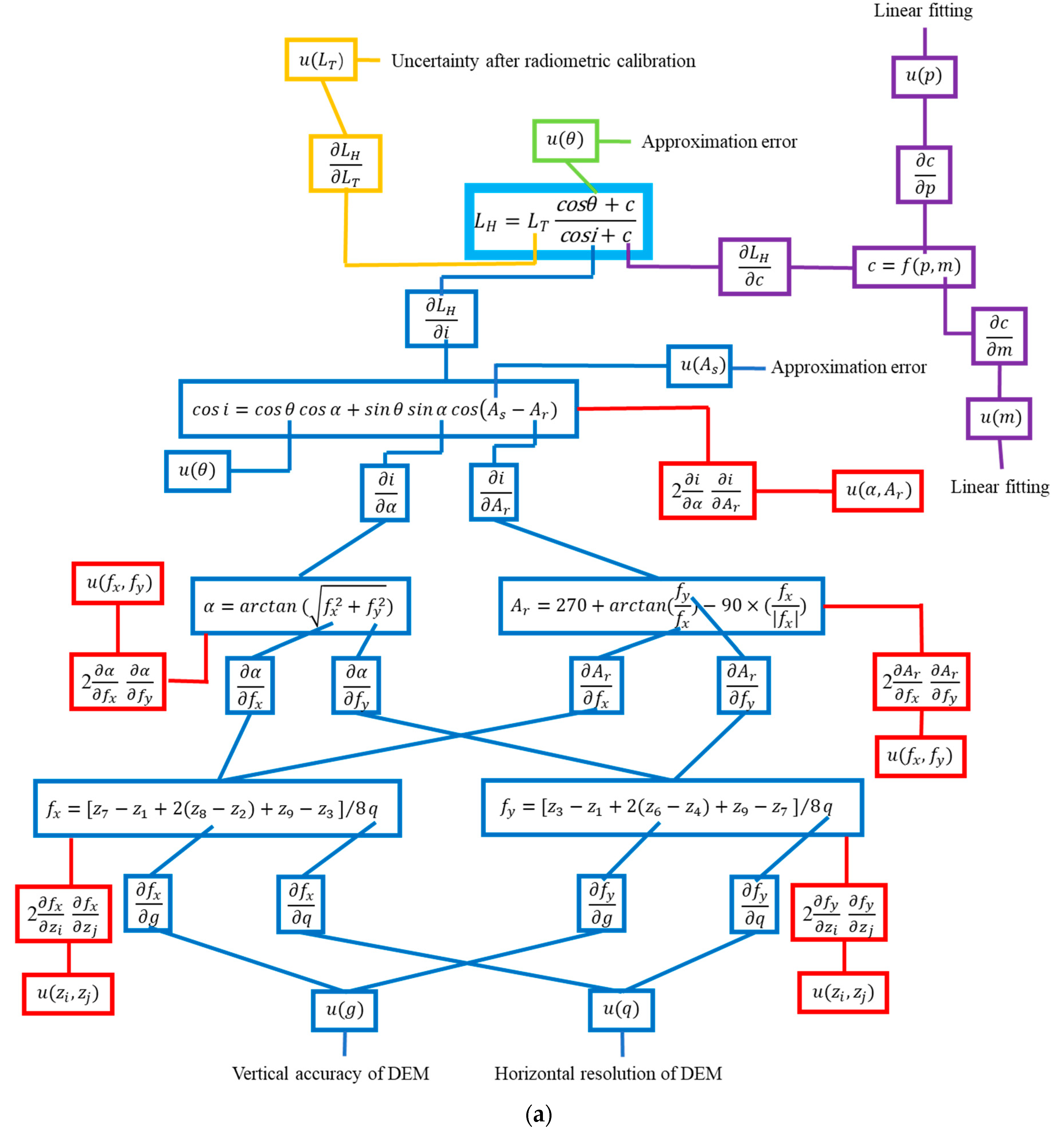
According to the data link in Section 2.1, the uncertainty propagation chain of the two topographic correction results are shown in Figure 3a,b. The uncertainty sources can be traced back to the uncertainty of at-sensor radiance after radiometric calibration, the vertical accuracy of DEM, the horizontal resolution of DEM, the approximation errors of solar illumination angles, and the uncertainty of linear fitting. In actual topographic correction for one scene, the solar illumination angles are consistent values for all pixels. The approximation errors introduce uncertainties into topographic correction, but their uncertainties are too small to be compared with other uncertainties. Therefore, the uncertainty introduced by solar illumination angles are considered negligible. The other four kinds of uncertainty sources should be evaluated by referring to actual conditions by type A or type B methods.

In addition, when combining the uncertainty, the correlations between each two input quantities should be considered. For C correction, the correlations among elevation values, between $f_x$ and $f_y$ and between $\alpha$ and $A_r,$ are considered. For Minnaert correction, the correlations among elevation values, between $f_x$ and $f_y$, between $\alpha$ and $A_r$, and between i and $\alpha$, are considered. They will be explained in detail in Section 2.2.3.

2.2.3. Uncertainties Introduced by Input Quantities

The uncertainties of $\alpha$, i, c, and k are from the uncertainty sources in Section 2.2.2. They are determined as follows:

1. Uncertainty of slope

The uncertainty of slope comes from the accuracy of DEM data.

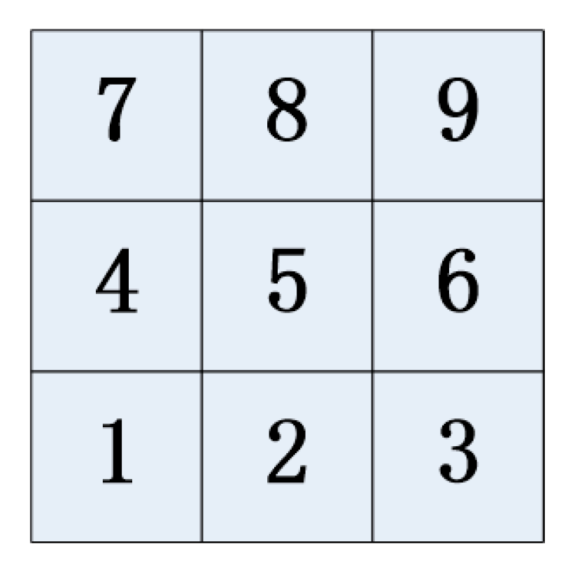
According to Equations (6) and (7), the slope and aspect are defined as functions of gradients at $x$ and $y$. It is clear that the key for slope and aspect computation is the calculation of $f_x$ and $f_y$. The common approach is to use a moving three-by-three window shown in Figure 4. Then $f_x$ and $f_y$ can be calculated as Equations (17) and (18), respectively, according to the 3FDWRSD algorithm [25]:

$$f_x=\left[z_7-z_1+2\left(z_8-z_2\right)+z_9-z_3\right]/8q,$$

(17)

$$f_y=\left[z_3-z_1+2\left(z_6-z_4\right)+z_9-z_7\right]/8q,$$

(18)

where $z_i$ is the elevation value of the grid i ($1\le i\le 9$) in a three-by-three moving window and q is the grid size.

When the uncertainty of elevation is known to be $u\left(g\right)$, the uncertainty of $z_i$ is $u\left(g\right)$. The uncertainty of q is known to be $u\left(q\right)$. Then the uncertainties associated with gradients are calculated as:

$$u_c\left(f_x\right)=\sqrt{{\displaystyle \sum }_{i=1,2,3,7,8,9}{\left[\frac{\partial f_x}{\partial z_i}\right]}^2{u}^2\left(g\right)+{[\frac{\partial f_x}{\partial q}]}^2{u}^2\left(q\right)+2{\displaystyle \sum }_{i=1,2,3,7,8,9}{\displaystyle \sum }_{j=1,2,3,7,8,9,j>i}\frac{\partial f_x}{\partial z_i}\frac{\partial f_x}{\partial z_j}u\left(z_i,z_j\right)},$$

(19)

$$u_c\left(f_y\right)=\sqrt{{\displaystyle \sum }_{i=1,3,4,6,7,9}{\left[\frac{\partial f_y}{\partial z_i}\right]}^2{u}^2\left(g\right)+{[\frac{\partial f_y}{\partial q}]}^2{u}^2\left(q\right)+2{\displaystyle \sum }_{i=1,3,4,6,7,9}{\displaystyle \sum }_{j=1,3,4,6,7,9,j>i}\frac{\partial f_y}{\partial z_i}\frac{\partial f_y}{\partial z_j}u\left(z_i,z_j\right)}.$$

(20)

The elevation values of grids $z_i$ are from the same dataset, hence they are correlated; and $u\left(z_i,z_j\right)$ is the covariance associated with the elevation values of every two grids.

Both $f_x$ and $f_y$ values are calculated from DEM data by 3FDWRSD, hence they are correlated. With reference to Equation (6), the combined standard uncertainty of slope is:

$$u_c\left(\alpha \right)=\sqrt{[\frac{\partial \alpha }{\partial f_x}{]}^2{u}_c^2\left(f_x\right)+[\frac{\partial \alpha }{\partial f_y}{]}^2{u}_c^2\left(f_y\right)+2\frac{\partial \alpha }{\partial f_x}\frac{\partial \alpha }{\partial f_y}u\left(f_x,f_y\right)}.$$

(21)

2. Uncertainty of solar incident angle

The computation of uncertainty of $A_r$ is similar to uncertainty of $\alpha$. Referring to Equation (7), the combined uncertainty of aspect is determined as:

$$u_c\left(A_r\right)=\sqrt{[\frac{\partial A_r}{\partial f_x}{]}^2{u}_c^2\left(f_x\right)+[\frac{\partial A_r}{\partial f_y}{]}^2{u}_c^2\left(f_y\right)+2\frac{\partial A_r}{\partial f_x}\frac{\partial A_r}{\partial f_y}u\left(f_x,f_y\right)}.$$

(22)

The correlation between $\alpha$ and $A_r$ should be considered because both $\alpha$ and $A_r$ are calculated from $f_x$ and $f_y$. With reference to Equation (5), the combined uncertainty of solar incident angle is:

$$u_c\left(i\right)=\sqrt{[\frac{\partial i}{\partial \alpha }{]}^2{u}_c^2\left(\alpha \right)+[\frac{\partial i}{\partial A_r}{]}^2{u}_c^2\left(A_r\right)+2\frac{\partial i}{\partial \alpha }\frac{\partial i}{\partial A_r}u\left(\alpha ,A_r\right)}.$$

(23)

3. Uncertainty of empirical parameter in C correction

The uncertainty of empirical parameter c comes from the process of linear fitting by the least square method.

For correlated variables $x$ and $y$, $\left(x_1,y_1\right),\left(x_2,y_2\right),\dots ,\left(x_n,y_n\right)$ is a set of samples whose size is n. The equation $\widehat{y}=\widehat{a}+\widehat{b}x$ is the unbiased estimation of $E\left(y\right)=a+bx$, which describes the linear relationship between $x$ and $y$. $a$ and $b$ denote the intercept and slope of the line; $E\left(y\right)$ denotes the expectation of $y$; $\widehat{a}$, $\widehat{b},$ and $\widehat{y}$ denote the estimates of $a$, $b,$ and $y, \mathrm{respectively}$. The least square estimate (LSE) of the linear coefficients is:

$$\{\begin{array}{c}\widehat{a}=\overline{y}-\widehat{b}\overline{x}\\ \widehat{b}=\frac{{{\displaystyle \sum }}_{i=1}^n\left(x_i-\overline{x}\right)(y_i-\overline{y})}{{{\displaystyle \sum }}_{i=1}^n{(x_i-\overline{x})}^2}\end{array},$$

(24)

where $\overline{x}=\frac{1}{n}{{\displaystyle \sum }}_{i=1}^n{x}_i$ denotes the mean of $x_i$, and $\overline{y}=\frac{1}{n}{{\displaystyle \sum }}_{i=1}^n{y}_i$ denotes the mean of $y_i$.

Referring to the properties of LSE in statistics [27], the variances of the estimated linear coefficients can be calculated as:

$$Var\left(\widehat{a}\right)=[\frac{1}{n}+\frac{{\overline{x}}^2}{{{\displaystyle \sum }}_{i=1}^n{(x_i-\overline{x})}^2}]·\frac{1}{n-2}{\displaystyle \sum }_{i=1}^n{(y_i-{\widehat{y}}_i)}^2,$$

(25)

$$Var\left(\widehat{b}\right)=\frac{\frac{1}{n-2}{{\displaystyle \sum }}_{i=1}^n{(y_i-{\widehat{y}}_i)}^2}{{{\displaystyle \sum }}_{i=1}^n{(x_i-\overline{x})}^2}.$$

(26)

The covariance of $\widehat{a}$ and $\widehat{b}$ is:

$$Cov\left(\widehat{a},\widehat{b}\right)=-\frac{\overline{\mathrm{x}}}{{{\displaystyle \sum }}_{i=1}^n{(x_i-\overline{x})}^2}·\frac{1}{n-2}{\displaystyle \sum }_{i=1}^n{(y_i-{\widehat{y}}_i)}^2,$$

(27)

The fitting result of C correction is as Equation (8). When $x=\mathit{cos}i$ and $y=L_T$, the uncertainties $u\left(m\right)$, $u\left(l\right),$ and $u\left(m,l\right)$ can be calculated as:

$$u\left(m\right)=\sqrt{\frac{\frac{1}{n-2}{{\displaystyle \sum }}_{i=1}^n{(y_i-\widehat{y_i})}^2}{{{\displaystyle \sum }}_{i=1}^n{(x_i-\overline{x})}^2}},$$

(28)

$$u\left(l\right)=\sqrt{[\frac{1}{n}+\frac{{\overline{x}}^2}{{{\displaystyle \sum }}_{i=1}^n{(x_i-\overline{x})}^2}]\cdot \frac{1}{n-2}{\displaystyle \sum }_{i=1}^n{(y_i-\widehat{y_i})}^2},$$

(29)

$$u\left(l,m\right)=-\frac{\overline{\mathrm{x}}}{{{\displaystyle \sum }}_{i=1}^n{(x_i-\overline{x})}^2}·\frac{1}{n-2}{\displaystyle \sum }_{i=1}^n{(y_i-{\widehat{y}}_i)}^2,$$

(30)

The combined uncertainty of empirical parameter c is synthesized as:

$$u_c\left(c\right)=\sqrt{{\left[\frac{\partial c}{\partial l}\right]}^2{u}^2\left(l\right)+{\left[\frac{\partial c}{\partial m}\right]}^2{u}^2\left(m\right)+2\frac{\partial c}{\partial l}\frac{\partial c}{\partial m}u\left(m,l\right)}.$$

(31)

4. Uncertainty of Minnaert constant

The uncertainty of Minnaert constant k can be calculated by the same linear regression process as that used for the uncertainty of empirical parameter in C correction. When setting $x=\mathit{log}(\mathit{cos}i\mathit{cos}\alpha )$ and $y=\mathit{log}(L_T\mathit{cos}\alpha )$, the combined uncertainty of empirical parameter k is:

$$u\left(k\right)=\sqrt{\frac{\frac{1}{n-2}{{\displaystyle \sum }}_{i=1}^n{(y_i-\widehat{y_i})}^2}{{{\displaystyle \sum }}_{i=1}^n{(x_i-\overline{x})}^2}}.$$

(32)

2.2.4. Total Combined Standard Uncertainty

After the steps in Section 2.2.3, the uncertainties associated with all of the input quantities are available. The total combined uncertainty can be obtained.

At the same time, to analyze the uncertainty results clearly, we need to clarify what the combined uncertainty is composed of. The combined variance (the square of the combined uncertainty) is the sum of different terms associated with input quantities. We define these terms as uncertainty components. The uncertainty component associated with each input quantity includes the uncertainty of the input quantity and its sensitivity. To compare the sensitivity of these components, we define the sensitivity coefficient in two different cases.

For C correction, all of the input quantities are independent. The total combined uncertainty of corrected radiance is:

$$u_c^C\left(L_H\right)=\sqrt{[\frac{\partial f}{\partial L_T}{]}^2{u}^2\left(L_T\right)+[\frac{\partial f}{\partial i}{]}^2{u}_c^2\left(i\right)+{[\frac{\partial f}{\partial c}]}^2{u}_c^2\left(c\right)}\mathrm{and}$$

(33)

the sensitivity coefficient is evaluated as $z_{x_i}=\frac{\partial f}{\partial x_i}$.

For Minnaert correction, as shown in Figure 3b, there is a correlation between solar incident angle and slope, so the combined standard uncertainty of corrected radiance is:

$$u_c^M\left(L_H\right)=\sqrt{[\frac{\partial f}{\partial L_T}{]}^2{u}^2\left(L_T\right)+[\frac{\partial f}{\partial i}{]}^2{u}_c^2\left(i\right)+[\frac{\partial f}{\partial \alpha }{]}^2{u}_c^2\left(\alpha \right)+[\frac{\partial f}{\partial k}{]}^2{u}_c^2\left(k\right)+2\frac{\partial f}{\partial i}\frac{\partial f}{\partial \alpha }u\left(i,\alpha \right)}.$$

(34)

We define $2\frac{\partial f}{\partial i}\frac{\partial f}{\partial \alpha }u\left(i,\alpha \right)$ as the correlated component and the others as independent components. For the independent component, $z_{x_i}={\left[\frac{\partial f}{\partial x_i}\right]}^2$; and for the correlated component, $z_{x_i,x_j}=2\frac{\partial f}{\partial x_i}\frac{\partial f}{\partial x_j}$. Then the components can be compared.

In the following section, to analyze the combined uncertainty results better, we take the absolute values to compare the magnitude of the sensitivity coefficients among different uncertainty components. When some input quantities are correlated, the combined variance (the square of the combined uncertainty) and its uncertainty components are presented.

2.2.5. Expanded Uncertainty

After the total combined standard uncertainty is obtained, the expanded uncertainty, denoted by $U$, can be obtained as Equation (35) by multiplying the combined standard uncertainty $u_c\left(L_H\right)$ by the coverage factor $k_p$:

$$U=k_p{u}_c\left(L_H\right).$$

(35)

Then the coverage interval associated with the corrected radiance, denoted as $L_H-U~L_H+U$, can be obtained.

It should be recognized that the expanded uncertainty provides no new information, but presents the previously available information in a different form. Ideally, one would like to choose a specific value of the coverage factor $k_p$ corresponding to a particular level of confidence p. This is not easy to do in practice because it requires extensive knowledge of the probability distribution characterized by the measurement result and its combined uncertainty.

For this problem, GUM provides a preferred method for its approximate solution according to the Central Limit Theorem. For topographic correction, the probability distribution cannot be exactly known. The uncertainties of input quantities and output do not meet the requirements of the Central Limit Theorem because the theorem requires all of the input quantities to be independent and the variance of output is much larger than any single component from a non-normally distributed input.

Therefore, the expanded uncertainty can only be roughly evaluated without the level of confidence. According to GUM, $k_p$ will be in the range from 2 to 3 in general. $k_p$ is determined as 2 in this study.

3. Exemplar Experiment

3.1. Experimental Area and Data Set

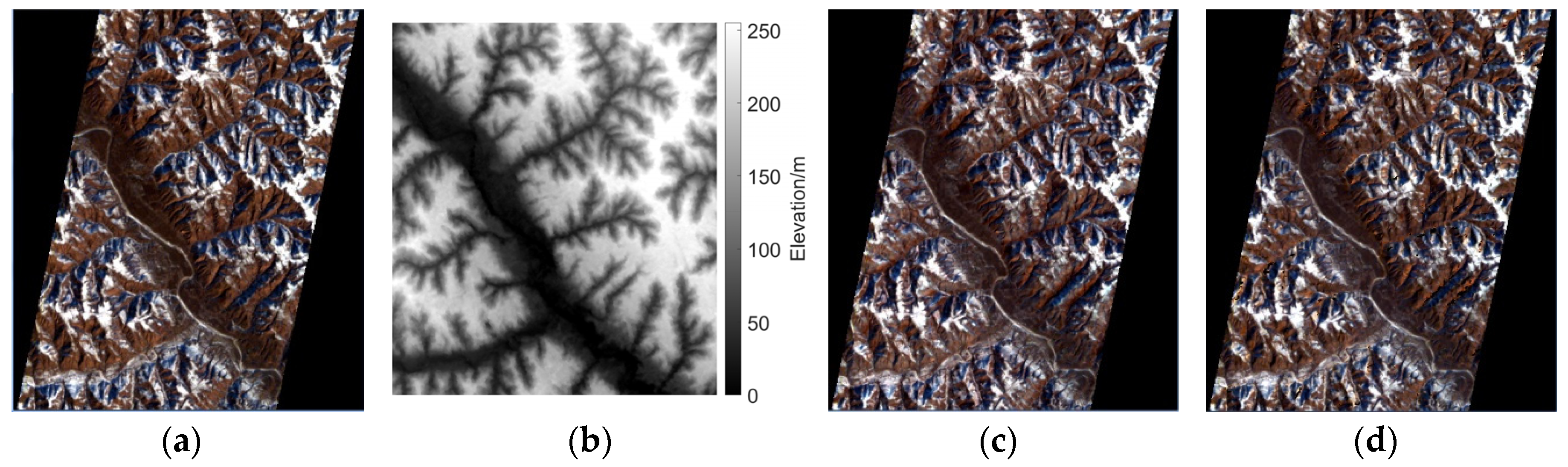
The selected experimental area was in the Loess Plateau near eastern Gansu and northern Shaanxi, China, covered with only snow and soil. The original data involved in the topographic correction included the hyperspectral at-sensor radiance (Figure 5a) and the DEM data (Figure 5b) of the area. The hyperspectral data used in this study was Hyperion data of EO-1 with a spatial resolution of 30 m, containing 196 bands, acquired on January 20, 2003. Its wavelength range was from 426 nm to 2395 nm. The DEM used in this study was ASTER GDEM data with a spatial resolution of 30 m and a scale of 1:250,000. The size of the image was 400 pixels by 348 pixels.

In topographic correction, the empirical coefficients were fitted first according to Equations (8)–(11). To calculate the empirical coefficients, 29,570 pixels on a sunlit slope were selected as samples. The samples were the same, but the fitting processes of each band were independent. Then the topographic correction was conducted for every pixel in each band. From the visual effect (Figure 5c,d), the undulating parts, such as the river course in the middle and the larger gullies on both sides of the river, were corrected to some degree, but inadequately.

The input data in topographic correction was radiance, not reflectance. Though the BRDFs of snow and soil differed markedly, it was not straightforward to classify the image data into different cover types. It should be clarified that though the surface was not classified before topographic correction, the coefficient fitting results were influenced by land cover, especially for Minnaert correction [28,29].

3.2. Uncertainty Analysis

3.2.1. Estimation of Uncertainty Sources

1. Estimation of uncertainty associated with at-sensor radiance

The at-sensor radiance was from the tier L1T data product of Hyperion after a series of pre-processing. The uncertainty of at-sensor radiance was roughly evaluated by the uncertainty after radiometric calibration, which is the key step in the pre-processing. The relative uncertainty of radiometric calibration $u_r\left(L_T\right)$ is usually 5%–8% [7]. In this study, the relative uncertainty of the at-sensor radiance was estimated as 5%. Therefore, the standard uncertainty of $L_T$ can be estimated as:

$$u\left(L_T\right)=u_r\left(L_T\right)\cdot L_T=5\%L_T.$$

(36)

2. Estimation of vertical uncertainty of DEM

The vertical uncertainty of DEM can be estimated by type B evaluation methods from the reference data of the handbook. According to GUM about type B evaluation method, the quoted uncertainty a can be assessed by information, which is usually uncertainty or half-width of the possible value interval of the measurand, from a manufacturer’s specification, calibration certificate, handbook, or other sources. When the probability distribution of the measurand and the level of confidence are known, the quoted uncertainty can be converted to the type B standard uncertainty divided by the factor.

According to ‘ASTER Global Digital Elevation Model Version 2—Summary of Validation Results’ [30], “the absolute vertical accuracy, expressed as a linear error at the 95% confidence level, is 17.01 meters”. The quoted accuracy gives the interval of the possible elevation values, which is ±17.01 m, and then the quoted uncertainty can be assessed by the half-width. According to GUM, if the quoted data has a percent level of confidence, unless otherwise indicated, one may assume it obeys normal distribution. Therefore, the vertical uncertainty of DEM can be estimated as:

$$u\left(g\right)=\frac{a}{k_{0.95}}.$$

(37)

By looking up the table, the factor $k_{0.95}$ of normal distribution is 1.96.

3. Estimation of horizontal uncertainty of DEM

The horizontal uncertainty can be estimated from the spatial resolution of DEM by type B evaluation methods. According to GUM, the distribution of the resolution can be considered as uniform distribution. Then the horizontal uncertainty can be evaluated as:

$$u\left(q\right)=\frac{resolution}{\sqrt{3}},$$

(38)

where $\sqrt{3}$ is the multiplier of uniform distribution with 100% level of confidence.

4. Estimation of uncertainties associated with solar illumination angles

As mentioned in Section 2.2.2, the uncertainties of solar illumination angles are introduced by approximation error between the center and the corners.

According to GUM, in the cases that it may be possible to estimate only bounds (upper limits $a_{+}$ and lower limits $a_{-}$) for the measurand, if there is no specific knowledge about the possible values of the measurand within the interval $a_{-}$ to $a_{+}$, one can assume that it obeys uniform distribution.

In this scene of image, the maximum errors of zenith and azimuth were 0.07° and 0.04°, respectively, and their relative uncertainties calculated by type B evaluation methods were less than 0.1% and less than 0.01%, respectively. The magnitudes of their uncertainties were not at the same level with uncertainties associated with other quantities. It was not much meaningful for topographic correction and thus the uncertainties of solar illumination angles were neglected.

3.2.2. Uncertainties of Input Quantities

The relative uncertainty of each input quantity was calculated to analyze its data quality (

Table 1. Relative uncertainty of input quantities.

Correction Model	${\mathit{u}}_{\mathit{r}}\left({\mathit{L}}_{\mathit{T}}\right)$	$\mathit{M}\mathit{d}\left({\mathit{u}}_{\mathit{r}}\left(\mathit{\alpha }\right)\right)$	$\mathit{M}\mathit{d}\left({\mathit{u}}_{\mathit{r}}\left({\mathit{A}}_{\mathit{r}}\right)\right)$	$\mathit{M}\mathit{d}\left({\mathit{u}}_{\mathit{r}}\left(\mathit{c}\right)\right)$$/\mathit{M}\mathit{d}\left({\mathit{u}}_{\mathit{r}}\left(\mathit{k}\right)\right)$
C correction	5%	62.47%	20.25%	5.50%
Minnaert correction				3.02%

). In uncertainty calculation, $u\left(\alpha \right)$, $u\left(A_r\right)$ relied on the location of each pixel, but had nothing to do with different bands; $u\left(c\right)$ and $u\left(k\right)$ were calculated band-by-band and at the same band, the uncertainty was the same; and $u\left(L_T\right)$ relied on both pixels and bands. Based on this situation, each pixel in each band had an uncertainty. In order to suppress the influence of extreme values, the median was used to estimate the uncertainty level of the input quantities. In Table 1, $Md\left(u_r\left(\alpha \right)\right)$, $Md\left(u_r\left(A_r\right)\right)$, $Md\left(u_r\left(c\right)\right),$ and $Md\left(u_r\left(k\right)\right)$ were respectively the median of the calculation results associated with $u_r\left(\alpha \right)$, $u_r\left(A_r\right)$, $u_r\left(c\right),$ and $u_r\left(k\right)$. As mentioned in Section 3.2.1, $u_r\left(L_T\right)$ was estimated as 5%.

It can be seen from Table 1 that $u_r\left(\alpha \right)$ and $u_r\left(A_r\right)$ were large, indicating that they were unstable. The relative uncertainty $u_r\left(\alpha \right)$, $u_r\left(A_r\right)$, $u_r\left(c\right),$ and $u_r\left(k\right)$ were analyzed further in detail.

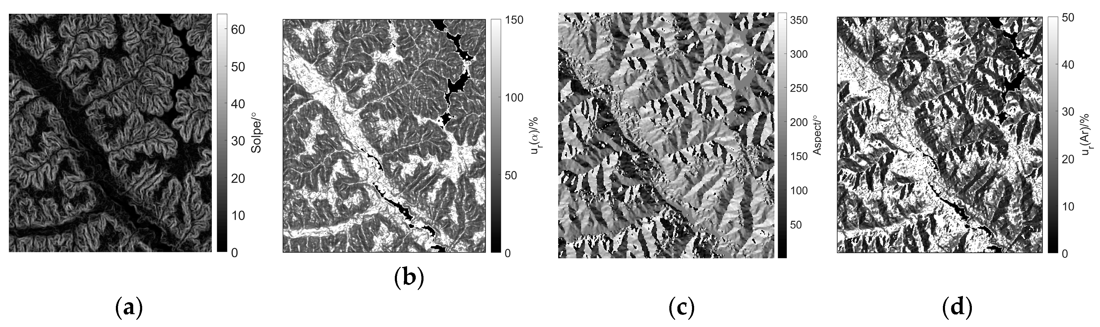
Parts a and b of Figure 6 are the visual images of slope and its uncertainty, respectively; and parts c and d of Figure 6 are the visual images of aspect and its uncertainty, respectively. The results indicated that in areas where the slope and the aspect values were smaller, the relative uncertainty was greater.

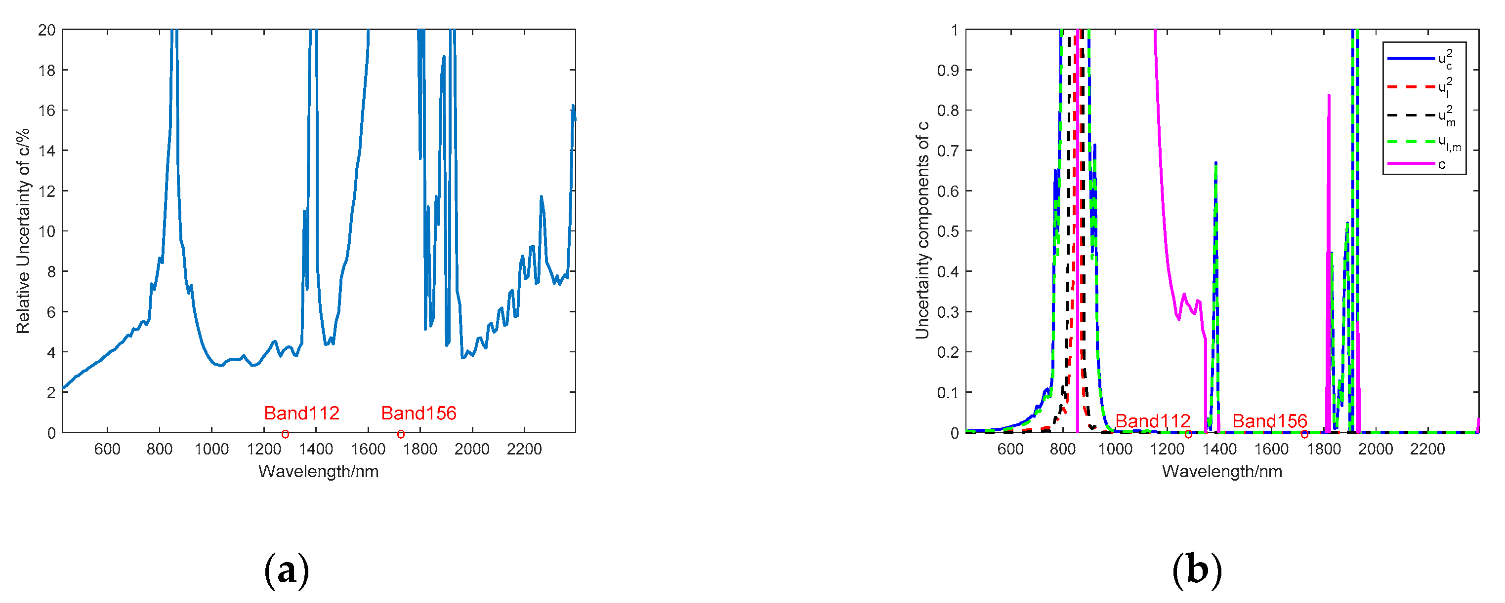
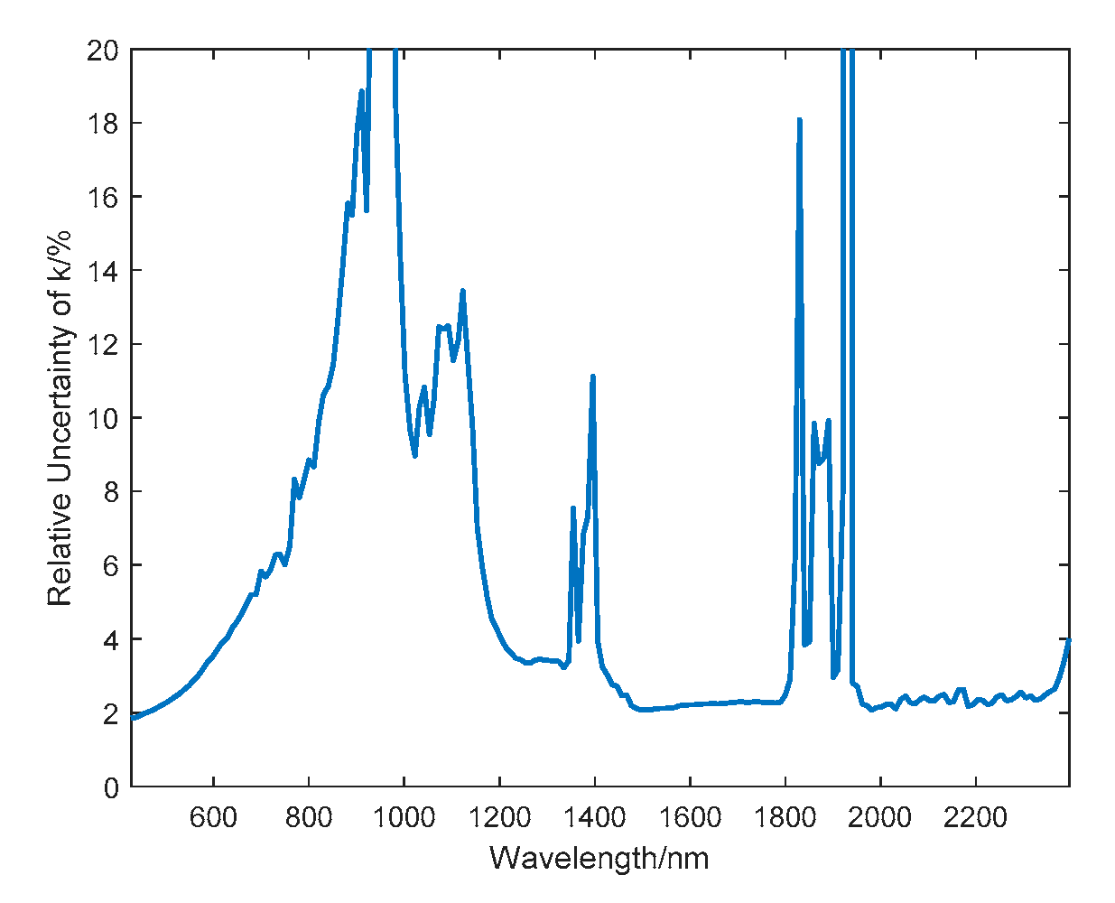
The relative uncertainties of empirical parameters were calculated band-by-band (Figure 7a and Figure 9). Uncertainties of the empirical parameter c and the Minnaert constant k were mainly derived from the linear regression and greatly influenced by the distribution of the samples. It should be noted that $u_c\left(c\right)$ was a combined uncertainty (Section 2.2.3). Figure 7b shows the combined variance (the square form of the combined uncertainty) and its uncertainty components to analyze the uncertainty of c better.

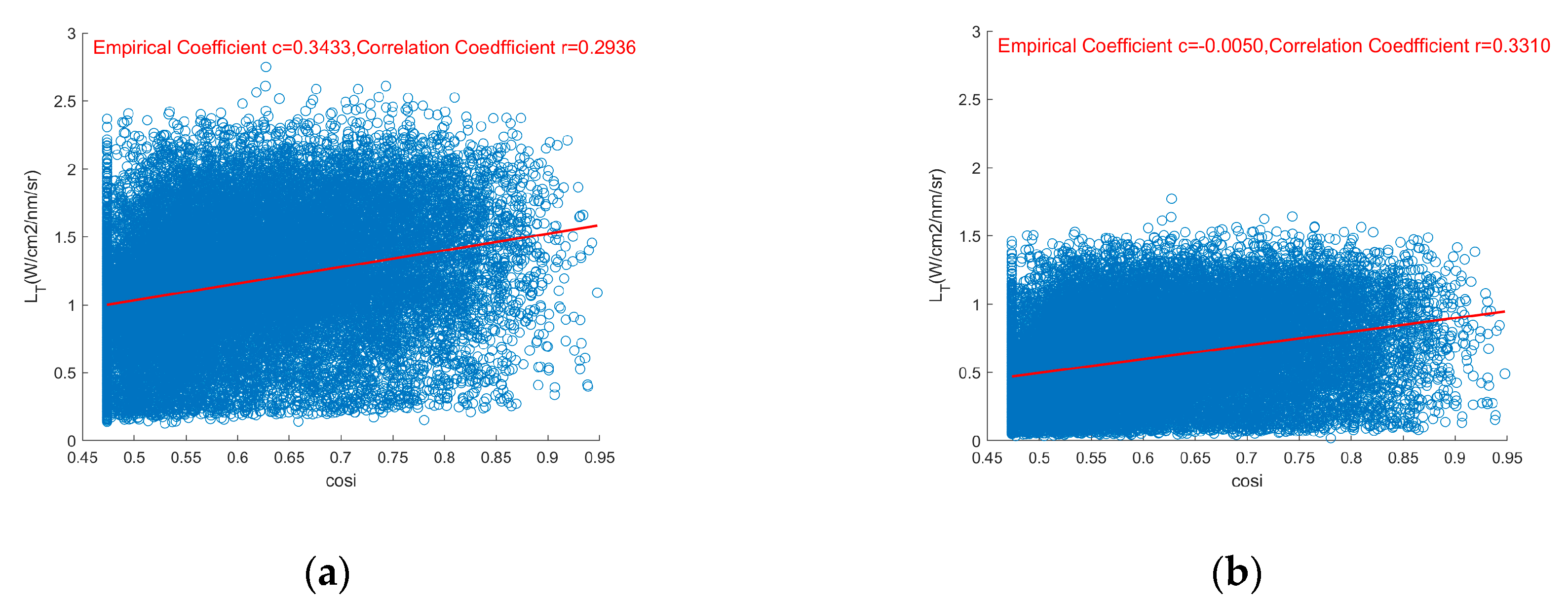
In the wavelength range of 400–2500 nm, there were five water vapor absorption bands: 820 nm, 940 nm, 1135 nm, 1400 nm, and 1900 nm, among which 1400 nm and 1900 nm were strong absorption bands. It can be seen from Figure 7 that the peaks around 820 nm, 1400 nm, and 1900 nm appeared in both relative and absolute uncertainties. The wavelength range of 1500–1800 nm had no features (Figure 7b), but high relative uncertainties (Figure 7a), only because the value of coefficient c dropped greatly in this wavelength range (pink line in Figure 7b). The distribution of sample points and fitting results in band 156 and band 112 are shown in Figure 8.

For Minnaert correction, the peaks of $u_r\left(k\right)$ around 940 nm, 1135 nm, 1400 nm, and 1900 nm shown in Figure 9 were all the water vapor absorption bands.

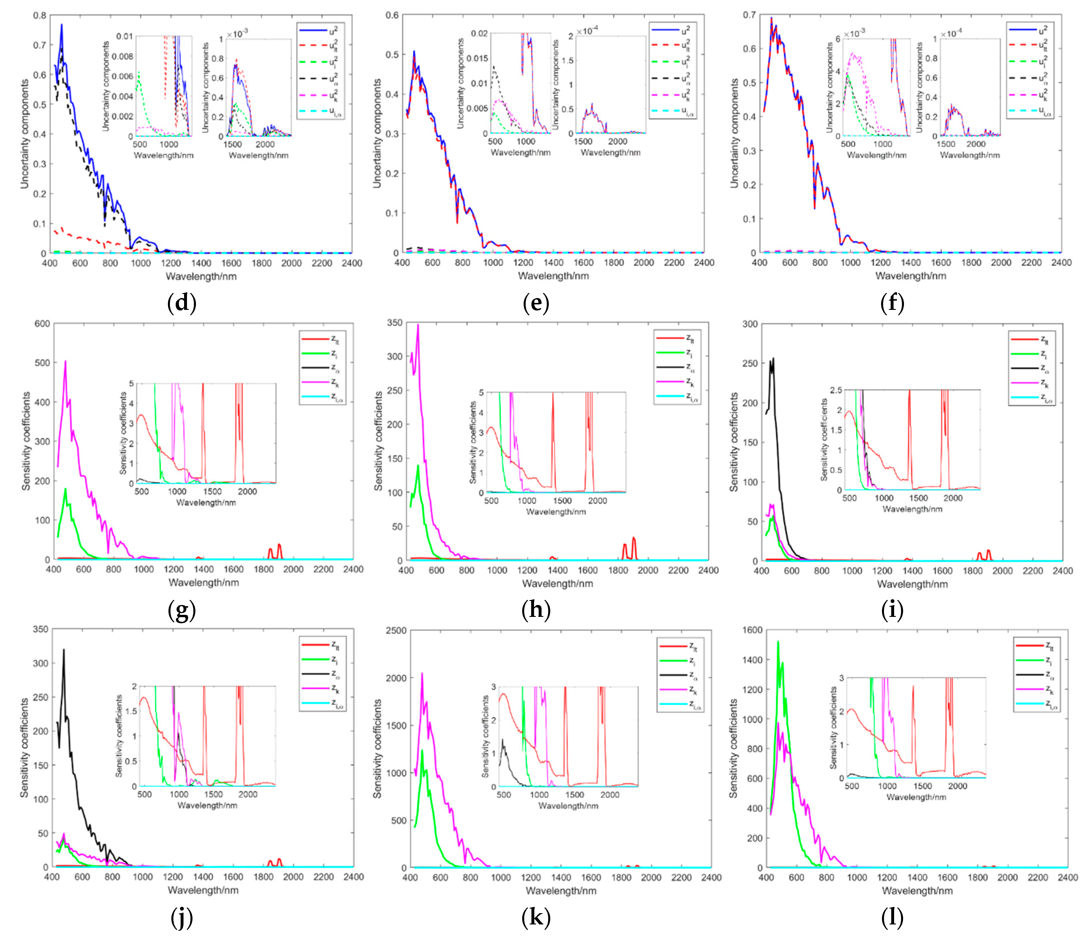
3.2.3. Uncertainty Components of the Total Combined Uncertainty

We selected six typical pixels of different cover types and different terrains for uncertainty analysis in this section. Information about these verification points is shown in

Table 2. Information about verification points.

Number	Coordinates	Slope (rad)	Aspect (rad)	Terrain	Cover Type
1	(76, 182)	0.0555	0.2268	flat, shaded	soil
2	(258, 214)	0.0395	4.3906	flat, sunlit	soil
3	(283, 236)	0.3923	1.4090	rugged, shaded	soil
4	(210, 258)	0.04396	3.6607	rugged, sunlit	soil
5	(303, 90)	0.0458	0.2450	flat, shaded	snow
6	(173, 288)	0.0314	2.3562	flat, sunlit	snow

. Under the cover type of soil, two flat points and two rugged points on a shaded slope and a sunlit slope were selected; under the cover type of snow, two points in shaded and sunlit flat areas were selected (snow falls in flat area). Figures 12 and 13 show the uncertainty components and sensitivity coefficients of the combined uncertainties.

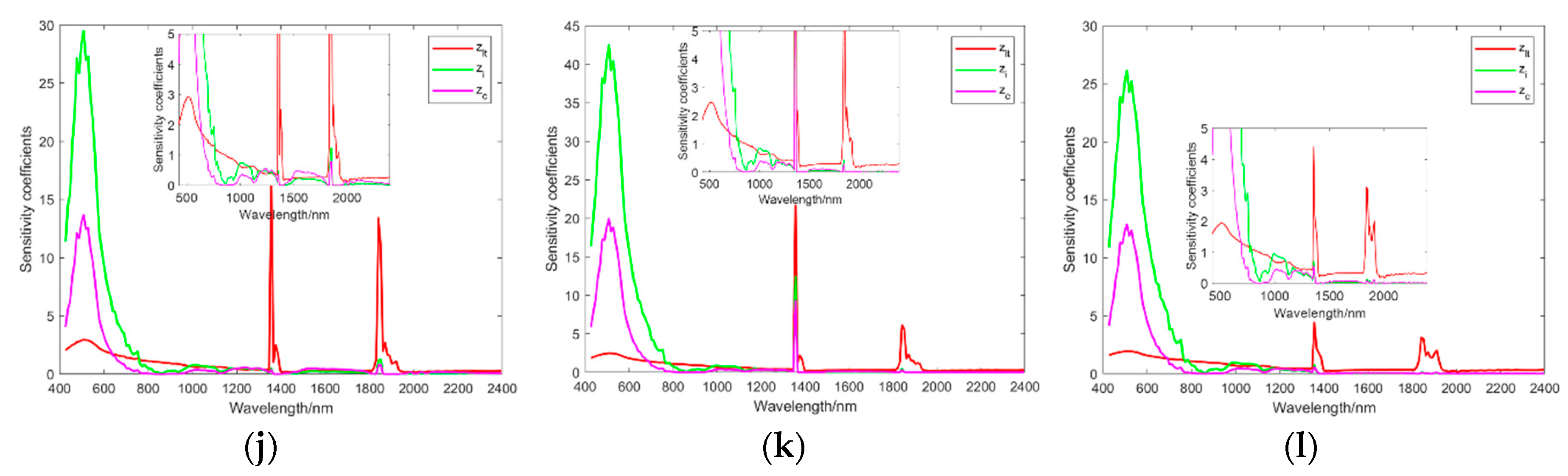
The uncertainty components considered in C correction were components associated with $L_T$, i, and c. They were independent. Figure 10 indicates the following about C correction: (i) For sensitivity coefficients, the trend of different conditions was consistent, which was to increase first, then decrease, and finally stabilize. They were similar to the trend of $L_T$. The bands around 1400 nm and 1900 nm were water vapor strong absorption bands, so they were not in the comparison. In bands below 600 nm, the input quantities whose sensitivity from high to low were i, c, and $L_T$. In bands between 800 nm to 2000 nm, their sensitivity coefficients were at the same level. In bands above 2000 nm, the input quantities whose sensitivity from high to low were $L_T$, c, and i. (ii) From the perspective of proportion, except point 4, the largest uncertainty component was always the uncertainty component associated with $L_T$. For the other five points, in bands below 800 nm, the uncertainty component associated with $L_T$ was the largest component, while the uncertainty component associated with i was the second largest component, and the uncertainty component associated with c was the smallest component; in bands between 800 nm and 1400 nm, the uncertainty component associated with c became the second largest one; in bands above 1400 nm, the uncertainty component associated with $L_T$ dominated the total combined uncertainty of the corrected result. (iii) From the perspective of different terrains, when the terrain was rugged and sunlit, the proportion of uncertainty component associated with i increased. The uncertainty of i was combined by uncertainties associated with slope and aspect. The result showed that when both slope and aspect were large (point 4, Figure 10d,j), the proportion of uncertainty component associated with i became the largest in bands below 600 nm. It should be noted that the terrain can affect the total combined uncertainty markedly in bands below 600 nm, because the sensitivity coefficient of i only dominated in bands below 600 nm. (iv) From the perspective of different cover types, there was nearly no difference.

The uncertainty components considered in Minnaert correction were independent uncertainty components associated with $L_T$, $\alpha$, i, and k, and the correlated uncertainty component between $\alpha$ and i. Figure 11 indicates the following about Minnaert correction: (i) Comparing the uncertainty results of the same cover type, but different terrain conditions: The uncertainty result changed markedly when the terrain condition changed. Comparing points covered with soil (points 1, 2, 3, and 4): When the terrain was flat, the uncertainty component associated with $L_T$ dominated the proportion of components and the sensitivity coefficients associated with k and i were the largest two components; when the terrain was rugged, the uncertainty component associated with $\alpha$ dominated the proportion of components and the uncertainty component associated with $L_T$ became the second largest component. Besides, the sensitivity coefficient associated with $\alpha$ became the largest and the sensitivity coefficients associated with k and i dropped to the second and the third largest components. Comparing points covered with snow (points 5 and 6): The two points were both in a flat area. When the aspects of them were different, the sensitivity coefficients differed. The sensitivity coefficient associated with i became the largest. (ii) Comparing the uncertainty results of the same terrain condition, but different cover types (points 1, 2, 5, and 6): The sensitivity coefficients of snowy points were influenced by the different aspects, in particular, the sensitivity coefficient associated with i. It may be because Minnaert correction considers non-Lambertian properties and the directional reflectance characteristics of snow and soil are different [31].

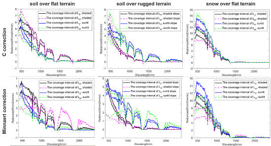
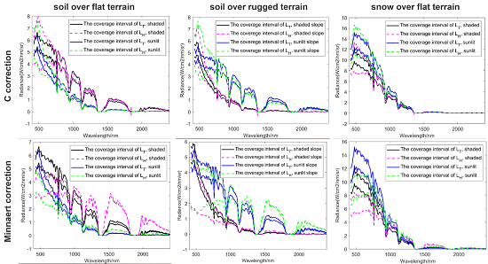
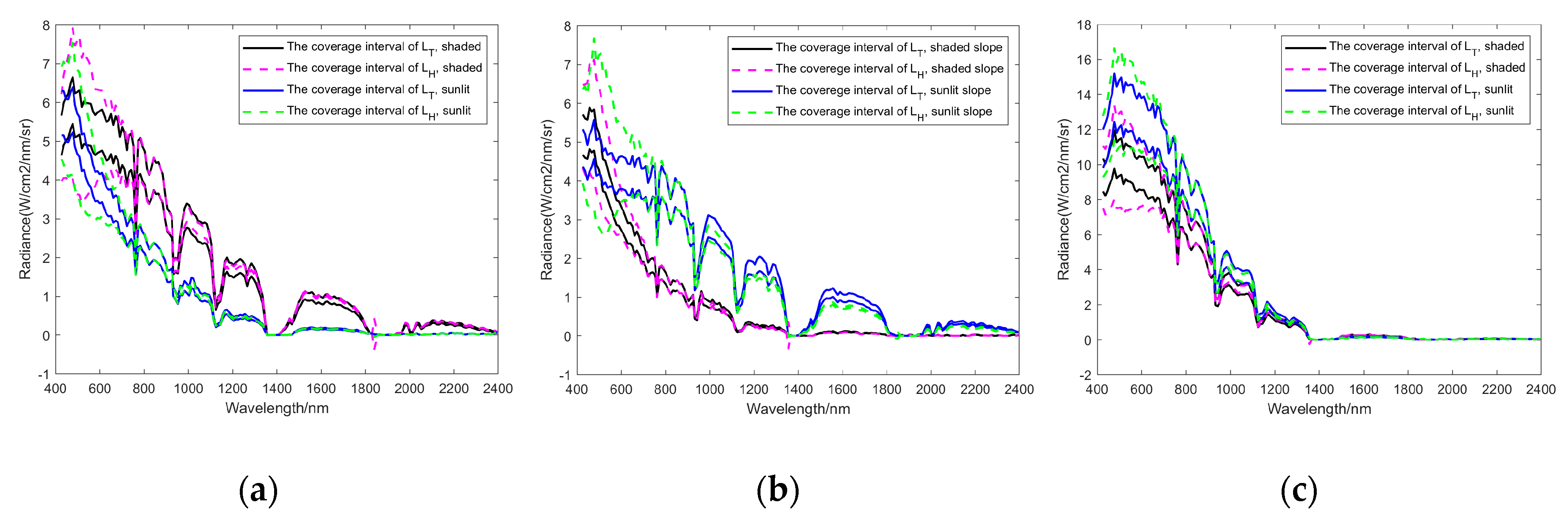
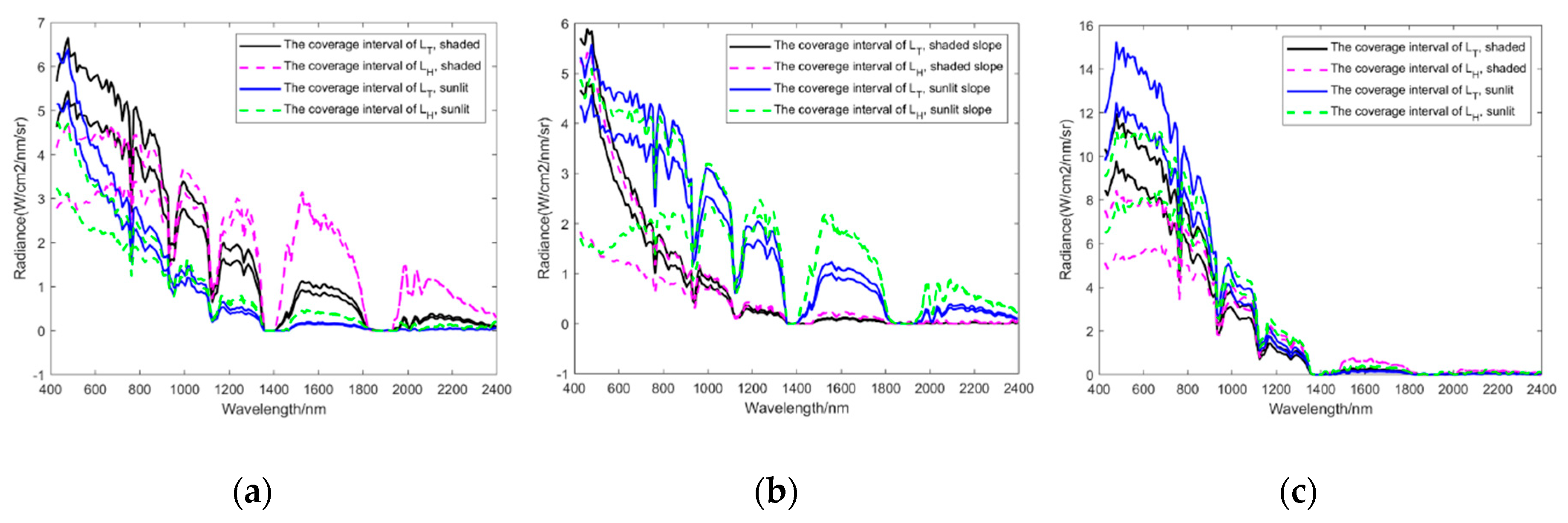
3.2.4. Uncertainty of the Corrected Radiance

The expanded uncertainty results of corrected radiance are shown in coverage intervals in Figure 12 (C correction) and Figure 13 (Minnaert correction). The two figures show the uncertainty coverage intervals of the six verification points before and after topographic correction, where the solid and dashed lines represent uncertainty coverage intervals before and after topographic correction, respectively. It can be seen that the uncertainty coverage intervals of radiance expanded after topographic correction, indicating that the DEM data and the topographic correction model introduced uncertainty. Combined with the analysis of Section 3.2, the expansion was due to the comprehensive impact of uncertainty components associated with input quantities propagating via correction models. It should be noted that the coverage intervals of C correction and Minnaert correction did not overlap well because the differences of the two correction methods caused systematic errors. The systematic errors of the correction models were not considered in our uncertainty results.

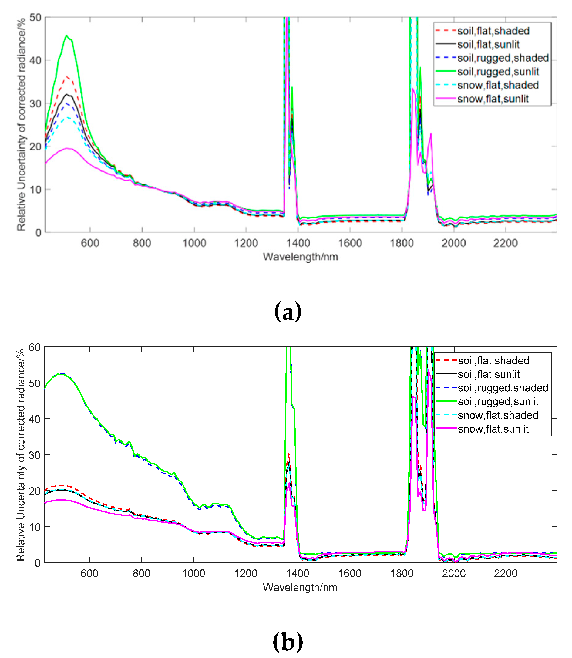
To analyze the uncertainty results removing the effect of the radiance value itself, the relative uncertainties (radio of the expanded uncertainty and the corrected radiance) of the six verification points are shown in Figure 14. From the perspective of spectral dimension, the relative uncertainties in bands around 1400 nm and 1900 nm were disturbed by strong water vapor absorption. Except these bands, the relative uncertainties of the six different conditions were close and relatively small in bands above 900 nm for C correction, while the relative uncertainties of the six different conditions were close and relatively small in bands above 1400 nm for Minnaert correction. In bands below 900 nm for C correction and below 1400 nm for Minnaert correction, the relative uncertainties were large, indicating that the data quality of the corrected radiance was poor in these bands.

The relative uncertainties of the snowy points were the smallest compared to points covered with soil, in both C correction and Minnaert correction. It indicated that the lower the radiance values, the larger the relative uncertainties.

For C correction, the point covered with soil and on the sunlit slope over a rugged terrain (green, solid line in Figure 14a) had the largest relative uncertainty, while for Minnaert correction, the points covered with soil over a rugged terrain, whatever the aspect was (green, solid line, and blue dashed line in Figure 14b), had the largest relative uncertainty. It indicated that from the perspective of spatial dimension, the uncertainties of the points whose terrains were rugged and aspect was sunlit were poor after C correction, while the uncertainties of the points over rugged terrains were poor after Minnaert correction.

4. Discussion

From the uncertainty results of the corrected radiance (Figure 14), we found that (i) the relative uncertainty of the cover types with lower radiance value was larger for both C and Minnaert corrections, (ii) the rugged terrain increased the uncertainty of the corrected radiance, and (iii) the uncertainty of the topographic corrected radiance was poor in bands below 1400 nm.

Over rugged terrains, the uncertainty of corrected radiance after C and Minnaert corrections increased in different situations. For C correction, the uncertainty component associated with i, which is related to terrain, was an important component of the total combined uncertainty associated with corrected radiance. It was combined by uncertainties associated with $\alpha$ and $A_r$. When the terrain was rugged and the aspect was sunlit, the proportion of uncertainty component associated with i increased markedly (Figure 10d). For Minnaert correction, the uncertainty component associated with i and the uncertainty component associated with $\alpha$, which are related to terrain, directly participated in the combination of the total combined uncertainty associated with corrected radiance. The uncertainty introduced by $\alpha$ had a bigger effect on the total combined uncertainty after Minnaert correction compared to C correction. When the terrain was rugged, whatever the aspect was, the proportion of uncertainty component associated with $\alpha$ increased markedly (Figure 11c,d). In summary, the rugged terrain increased the uncertainty of the corrected radiance substantially both for C and Minnaert corrections. It was meaningful to reduce the uncertainty of $\alpha$ and $A_r$ for topographic correction.

The poor uncertainty of the corrected radiance in bands below 1400 nm could be attributed to the following reasons. The uncertainty components associated with $L_T$, $\alpha ,$ and $A_r$ were the key components of the total combined uncertainty associated with corrected radiance. Generally speaking, the uncertainty component associated with $L_T$ dominated the combined uncertainty when the terrain was flat, while the uncertainty components associated with topographic parameters $\alpha$ and $A_r$ dominated the combined uncertainty when the terrain was rugged. The poor uncertainty of the corrected radiance in bands below 1400 nm was mainly because of the poor uncertainty components associated with $L_T$, $\alpha ,$ and $A_r$ in bands below 1400 nm.

The uncertainty component associated with each input quantity was disassembled into the uncertainty and its sensitivity for further analysis. The spectral trend of all of these sensitivity coefficients (of $L_T$, $\alpha$, and $A_r$) was related to the trend of $L_T$. The $L_T$ value decreased in bands above 1400 nm compared to the value in bands below 1400 nm, and a similar trend was observed for the sensitivity coefficients. For the uncertainty component associated with $\alpha$ and $A_r,$ the uncertainties of $\alpha$ and $A_r$ had nothing to do with wavelength, so the trend of sensitivity contributed to the larger values of uncertainty components associated with $\alpha$ and $A_r$ in bands below 1400 nm (actually below 600 nm in C correction and below 1200 nm in Minnaert correction). For the uncertainty component associated with $L_T$, the sensitivity coefficient also decreased due to the decrease of $L_T$ (only comparing value above 1400 nm with value below 1400 nm roughly). Besides, the uncertainty of $L_T$ was evaluated by 5% of the radiance value, so the trend of radiance value also relied on the trend of $L_T$. The two reasons contribute to the larger values of uncertainty components associated with $L_T$ in bands below 1400 nm.

The abovementioned spectral differences of the uncertainty components associated with $L_T$, $\alpha ,$ and $A_r$ would explain why the uncertainty was poor in bands below 1400 nm, while the uncertainty was relatively acceptable in bands above 1400 nm (except in water vapor absorption bands). It was meaningful to reduce the uncertainties of $L_T$, $\alpha$ and $A_r$ for reducing the total combined uncertainty associated with corrected radiance because the sensitivity was determined by the mathematical relationships in measurement equations.

According to the results of the uncertainty analysis, uncertainty can be reduced and data quality can be improved. In particular, the uncertainty in bands below 1400 nm and the uncertainty of low-radiance cover type should be paid more attention.

The uncertainty of $L_T$ was mainly from the uncertainty of radiance after radiometric calibration. Therefore, higher precision of radiometric calibration was needed, especially in bands below 1400 nm.

The uncertainties of $\alpha$ and $A_r$ were derived from the vertical accuracy and horizontal resolution of DEM by the 3FDWRSD algorithm. The possible approaches to reduce the uncertainty of $\alpha$ and $A_r$ can include: (i) The use of DEM data with higher accuracy and precision. This study used DEM data with a vertical accuracy of 17.01 m and a horizontal resolution of 30 m. DEM with higher accuracy and resolution would make sense to uncertainty reduction. (ii) The selection of a larger grid size of the moving window. In the 3FDWRSD algorithm, the grid size q was adjustable. According to Equations (20) and (21), the selection of a larger grid size can reduce the uncertainty of $f_x$ and $f_y$. It should be noted that the selection of grid size may also affect the accuracy of $\alpha$ and $A_r$. Therefore, the appropriate selection of the grid size is pivotal. (iii) The use of other algorithms for calculating slope and aspect. It should be noted that this study focused on the uncertainty propagation via mathematical models, but the actual uncertainty sources of the algorithms for calculating slope and aspect also include the error caused by the algorithm model itself [15]. Improving the data quality of slope and aspect is more complicated and needs further research.

5. Conclusions

In this study, the GUM method was used to analyze the uncertainty propagation of topographic correction models. We summed up the data links of the C and Minnaert models and traced the uncertainty sources back to the uncertainty of at-sensor radiance after radiometric calibration, the vertical accuracy of DEM, the horizontal resolution of DEM, the approximation errors of solar illumination angles, and the uncertainty of linear fitting. We proposed the uncertainty analysis method for semi-empirical topographic correction models and preliminarily established the uncertainty propagation chains.

We applied the uncertainty analysis method to a set of EO-1 Hyperion data acquired in the Loess Plateau, China, in winter, which actually contains two surface cover types, namely, soil and snow. We obtained the uncertainty characteristics of terrain-corrected hyperspectral radiance by analyzing the uncertainties associated with input quantities, the components of the total combined uncertainty, and the uncertainty associated with corrected radiance. The conclusions were: (i) The relative uncertainty of the cover types with lower radiance value was larger for both C and Minnaert corrections. (ii) The uncertainty of the topographic corrected radiance was poor in bands below 1400 nm. It was because the trend of $L_T$ value had influence on the sensitivity of uncertainty components and the uncertainty of $L_T$. The $L_T$ value was higher in bands below 1400 nm compared to the value in bands above 1400 nm. (iii) The uncertainty components associated with $L_T$, $\alpha ,$ and $A_r$ dominated the total combined uncertainty of corrected radiance. Over a rugged terrain, the uncertainty components associated with $\alpha$ and $A_r$ increased the uncertainty of the corrected radiance. It was meaningful to reduce the uncertainty of $L_T$, $\alpha$, and $A_r$ for reducing the uncertainty of corrected radiance and improving the data quality.

Besides, the uncertainty information of remote sensing products is usually limited. More thorough uncertainty indexes are expected to be reported.

References

- BIPM; IEC; IFCC; ILAC; ISO; IUPAC; IUPAP; OIML. Evaluation of Measurement Data-Guide to the Expression of Uncertainty in Measurement. Available online: http://www.bipm.org/utils/common/documents/jcgm/JCGM_100_2008_E.pdf (accessed on 6 January 2020).
- Fox, N. A Guide to Expression of Uncertainty of Measurements. Available online: http://qa4eo.org/docs/QA4EO-QAEO-GEN-DQK-006_v4.0.pdf (accessed on 6 January 2020).
- Fidelity and Uncertainty in Climate Data Records from Earth Observations. Available online: http://www.fiduceo.eu/ (accessed on 6 January 2020).
- Woolliams, E.; Hueni, A.; Gorrono, J. Intermediate Uncertainty Analysis for Earth Observation (Instrument Calibration): NPL Training Course Textbook. Available online: http://www.emceoc.org/documents/uaeo-int-trg-course.pdf (accessed on 2 September 2019).
- Chrien, T.G.; Green, R.O.; Eastwood, M.L. Accuracy of the spectral and radiometric laboratory calibration of the Airborne Visible/Infrared Imaging Spectrometer. In Proceedings of the SPIE, Orlando, FL, USA, 1 September 1990. [Google Scholar]
- Bachmann, M.; Makarau, A.; Segl, K.; Richter, R. Estimating the influence of spectral and radiometric calibration uncertainties on EnMAP data products-examples for ground reflectance retrieval and vegetation indices. Remote Sens. Basel 2015, 7, 10689–10714. [Google Scholar] [CrossRef] [Green Version]
- Li, Y.; Yu, B.; Wang, Y.; Fang, W. Measurement chain of influence quantities and uncertainty of radiometric calibration for imaging spectrometer. Opt. Precis. Eng. 2006, 14, 822–828. (In Chinese) [Google Scholar]
- Jia, G.; Zhao, H.; Li, H. Uncertainty propagation algorithm from the radiometric calibration to the restored earth observation radiance. Opt. Express 2014, 22, 9442–9449. [Google Scholar]
- Honkavaara, E.; Markelin, L.; Hakala, T.; Peltoniemi, J. The metrology of directional, spectral reflectance factor measurements based on area format imaging by UAVs. Photogramm. Fernerkun. 2014, 2014, 175–188. [Google Scholar] [CrossRef]
- Jia, G.; Xue, Q.; Zhao, H. Uncertainty analysis for surface reflectance retrieved from hyperspectral remote sensing image using empirical line method. In Proceedings of the IEEE Conference on Hyperspectral Image and Signal Processing: Evolution in Remote Sensing, Amsterdam, The Netherlands, 23–26 September 2018. [Google Scholar]
- Teillet, P.M.; Guindon, B.; Goodenough, D.G. On the slope-aspect correction of multispectral scanner data. Can. J. Remote Sens. 1982, 8, 84–106. [Google Scholar] [CrossRef] [Green Version]
- Meyer, P.; Itten, K.I.; Kellenberger, T.; Sandmeier, S. Radiometric corrections of topographically induced effects on Landsat TM data in an alpine environment. ISPRS J. Photogramm. 1993, 48, 17–28. [Google Scholar] [CrossRef]
- Vincini, M.; Reeder, D.; Frazzi, E. An empirical topographic normalization method for forest TM data. In Proceedings of the IEEE International Geoscience and Remote Sensing Symposium, Toronto, ON, Canada, 24–28 June 2002. [Google Scholar]
- Gao, Y.; Zhang, W. Variable empirical coefficient algorithm for removal of topographic effects on remotely sensed data from rugged terrain. In Proceedings of the IEEE International Geoscience and Remote Sensing Symposium, Barcelona, Spain, 23–28 July 2007. [Google Scholar]
- Civco, D.L. Topographic normalization of Landsat thematic mapper digital imagery. Photogramm. Eng. Rem. Sens. 1989, 55, 1303–1309. [Google Scholar]
- Baraldi, A.; Gironda, M.; Simonetti, D. Operational two-stage stratified topographic correction of spaceborne multispectral imagery employing an automatic spectral-rule-based decision-tree preliminary classifier. IEEE Trans. Geosci. Remote 2010, 48, 112–146. [Google Scholar] [CrossRef]
- Zhang, W. Water Resource and Hydrological Processes Studies on the Urumqi River Basin, Tianshan, China by Means of Remote Sensing and GIS Techniques. Ph.D. Thesis, Nagoya University, Nagoya, Japan, 2000. [Google Scholar]
- Gu, D.; Gillespie, A. Topographic normalization of Landsat TM images of forest based on subpixel sun-canopy-sensor geometry. Remote Sens. Environ. 1998, 64, 166–175. [Google Scholar] [CrossRef]
- Proy, C.; Tanre, D.; Deschamps, P.Y. Evaluation of topographic effects in remotely sensed data. Remote Sens. Environ. 1989, 30, 21–32. [Google Scholar] [CrossRef]
- Sandmeier, S.; Itten, K.I. A physically-based model to correct atmospheric and illumination effects in optical satellite data of rugged terrain. IEEE Trans. Geosci. Remote 1997, 35, 708–717. [Google Scholar] [CrossRef] [Green Version]
- Soenen, S.A.; Peddle, D.R.; Coburn, C.A. SCS+C: A modified sun-canopy-sensor topographic correction in forested terrain. IEEE Trans. Geosci. Remote 2005, 43, 2148–2159. [Google Scholar] [CrossRef]
- Smith, J.A.; Lin, T.L.; Ranson, K.L. The Lambertian assumption and Landsat data. Photogramm. Eng. Rem. S. 1980, 46, 1183–1189. [Google Scholar]
- Vincini, M.; Reeder, D.; Frazzi, E. Seasonal Landsat TM data topographic dependence in rugged deciduous forest areas. In Proceedings of the Analysis of Multi-Temporal Remote Sensing Images-the First International Workshop on Multitemp, Trento, Italy, 13–14 September 2001. [Google Scholar]
- Zhou, Q.; Liu, X. Analysis of errors of derived slope and aspect related to DEM data properties. Comput. Geosci. 2004, 30, 369–378. [Google Scholar] [CrossRef]
- Horn, B.K. Hill shading and the reflectance map. Proc. IEEE 1981. [Google Scholar] [CrossRef] [Green Version]
- International Vocabulary of Metrology—Basic and General Concepts and Associated Terms (VIM 3rd edition). Available online: https://www.bipm.org/utils/common/documents/jcgm/JCGM_200_2012.pdf (accessed on 6 January 2020).
- Sun, R.H. Applied Mathematical Statistics, 3rd ed.; Science Press: Beijing, China, 2014. (In Chinese) [Google Scholar]
- Bishop, M.P.; Colby, J.D. Anisotropic reflectance correction of SPOT-3 HRV imagery. Int. J. Remote Sens. 2002, 23, 2125–2131. [Google Scholar] [CrossRef]
- Bishop, M.P.; Shroder, J.F., Jr.; Colby, J.D. Remote sensing and geomorphometry for studying relief production in high mountains. Geomorphology 2003, 55, 345–361. [Google Scholar] [CrossRef] [Green Version]
- ASTER Global Digital Elevation Model Version 2- Summary of Validation Results. Available online: https://lpdaac.usgs.gov/documents/220/Summary_GDEM2_validation_report_final.pdf (accessed on 6 January 2020).
- Nolin, A.W.; Liang, S. Progress in bidirectional reflectance modeling and applications for surface particulate media: Snow and soils. Remote Sens. Rev. 2000, 18, 307–342. [Google Scholar] [CrossRef]
Figure 1.
Geometric relationship of “Sun–surface–sensor”.
Figure 2.
Data link of the two topographic correction models.
Figure 3.
Uncertainty propagation chain of: (a) C correction; (b) Minnaert correction.
Figure 4.
Schematic diagram of a three-by-three moving window.
Figure 5.
The original data and corrected results: (a) RGB hyperspectral image to be corrected; (b) digital elevation model (DEM) image; (c) RGB radiance image after C correction; (d) RGB radiance image after Minnaert correction.
Figure 6.
Visual images of (a) slope and (b) its relative uncertainty; visual images of (c) aspect and (d) its relative uncertainty.
Figure 7.
Absolute uncertainty and relative uncertainty of parameter c. (a) Relative uncertainty; (b) absolute uncertainty and its components. In subplot (b), the blue solid line is the combined variance of c; the dashed lines are the uncertainty components associated with intercept l (red), slope m (black), and the correlation component between l and m (green); the pink solid line is the value of c.
Figure 8.
The coefficient fitting of (a) band112 and (b) band 156. Significance level is 0.10.
Figure 9.
Relative uncertainty of parameter k.
Figure 10.
Uncertainty components of C correction. The subplots (a–f) and (g–l) represent the uncertainty components and sensitivity coefficients associated with input quantities of the six verification points, respectively; In each subplot of (a–f), the blue solid line is the total combined variance of corrected radiance after C correction; the dashed lines are the uncertainty components associated with (red), i (green), and c (pink). In each subplot of (g–l), the lines are the sensitivity coefficients associated with (red), i (green), and c (pink). Every subplot is zoomed in on y-axis as its inner plot to show local details of low-value points.
Figure 11.
Uncertainty components of Minnaert correction. The subplots (a–f) and (g–l) represent the uncertainty components and sensitivity coefficients associated with input quantities of the six verification points, respectively. In each subplot of (a–f), the blue solid line is the total combined variance of corrected radiance after Minnaert correction; the dashed lines are the uncertainty components associated with (red), i (green), (black), and k (pink), and the correlation components between i and (cyan). In each subplot of (g–l), the lines are the sensitivity coefficients associated with (red), i (green), (black), and k (pink), and the correlation components between i and (cyan). Every subplot is zoomed in on y-axis as its inner plot to show local details of low-value points.
Figure 12.
The uncertainty coverage intervals before and after C correction. (a) The coverage interval of soil over a flat terrain; (b) the coverage interval of soil over a rugged terrain; (c) the coverage interval of snow over a flat terrain. In each subplot, the solid and dashed lines are respectively the uncertainty coverage intervals before and after C correction; the black and pink lines are verification points on the shaded slope, while the blue and green lines are verification points on the sunlit slope.
Figure 13.
The uncertainty coverage intervals before and after Minnaert correction. (a) The coverage interval of soil over a flat terrain; (b) the coverage interval of soil over a rugged terrain; (c) the coverage interval of snow over a flat terrain. In each subplot, the solid and dashed lines are respectively the uncertainty coverage intervals before and after Minnaert correction; the black and pink lines are verification points on the shaded slope, while the blue and green lines are verification points on the sunlit slope.
Figure 14.
The relative uncertainties of the six verification points after (a) C correction; (b) Minnaert correction. In each subplot, the six points are respectively the pink dashed line (point 1), the black solid line (point 2), the blue dashed line (point 3), the green solid line (point 4), the cyan dashed line (point 5), and the pink solid line (point 5).