A New Model for Transfer Learning-Based Mapping of Burn Severity
by
 , , , ,
Zhong Zheng
1,2,3,4 ,
,
Jinfei Wang
2,*,
Bo Shan
2,
Yongjun He
2,
Chunhua Liao
2,
Yanghua Gao
3 and
Shiqi Yang
3 1
College of Resources and Environment, Chengdu University of Information Technology, Chengdu 610225, China
2
Department of Geography, The University of Western Ontario, London, ON N6A 5C2, Canada
3
Chongqing Institute of Meteorological Sciences, Chongqing 401147, China
4
School of Geographical Sciences, Southwest University, Chongqing 400715, China
*
Author to whom correspondence should be addressed.
Remote Sens. 2020, 12(4), 708; https://0-doi-org.brum.beds.ac.uk/10.3390/rs12040708
Submission received: 29 January 2020
/
Revised: 17 February 2020
/
Accepted: 19 February 2020
/
Published: 21 February 2020
(This article belongs to the Special Issue Advances in Remote Sensing of Post-fire Environmental Damage and Recovery Dynamics)
Abstract
:In recent years, global forest fires have occurred more frequently, seriously destroying the structural functions of forest ecosystem. Mapping the burn severity after forest fires is of great significance for quantifying fire’s effects on landscapes and establishing restoration measures. Generally, intensive field surveys across burned areas are required for the effective application of traditional methods. Unfortunately, this requirement could not be satisfied in most cases, since the field work demands a lot of personnel and funding. For mapping severity levels across burned areas without field survey data, a semi-supervised transfer component analysis-based support vector regression model (SSTCA-SVR) was proposed in this study to transfer knowledge trained from other burned areas with field survey data. Its performance was further evaluated in various eco-type regions of southwestern United States. Results show that SSTCA-SVR which was trained on source domain areas could effectively be transferred to a target domain area. Meanwhile, the SSTCA-SVR could maintain as much spectral information as possible to map burn severity. Its mapped results are more accurate (RMSE values were between 0.4833 and 0.6659) and finer, compared to those mapped by ∆NDVI-, ∆LST-, ∆NBR- (RMSE values ranged from 0.7362 to 1.1187) and SVR-based models (RMSE values varied from 1.7658 to 2.0055). This study has introduced a potentially efficient mechanism to map burn severity, which will speed up the response of post-fire management.

1. Introduction
Forests contain up to 80% of the planet’s above ground biomass carbon, which plays a very important role in maintaining the security of global ecosystem [1,2]. Annually, millions of hectares of global forest areas are severely damaged by fires [3]. Mapping the spatial distribution of damage levels not only facilitates the quantification of fire’s impact on landscapes, but also effectively guides the implementation of post-fire restoration efforts [4,5].
Burn severity is often considered a measure for describing fire’s impacts on forest landscape, which is commonly measured by a quantitative metric: composite burn index (CBI) [6,7]. For mapping the spatial distribution of this variable, the field survey method is supposed to be direct and accurate, but requires a great deal of time, money, and human resources [8]. With large-scale and low-cost characteristics, remote sensing-based methods can greatly improve the efficiency of mapping burn severity [9,10].
Generally, remote sensing-based methods for mapping burn severity include: predictor variables-based regression models [5,7,9], spectral mixture analysis [4,11], and radiative transfer models [6,12,13]. Regarding predictor variables, spectral indices are widely employed in most reported models [14,15,16,17,18,19,20,21,22]. One of spectral indices is the normalized burn ratio (NBR) which can be calculated from near- and shortwave-infrared spectral bands of remotely sensed data [17]. The differenced NBR (∆NBR) was further derived from pre- and post-fire images and it has been recognized as a reference for mapping burn severity [4,23]. Following that, a relative modification of ∆NBR (RdNBR) was developed to remove the burn severity misclassification of low vegetated pixels [24]. Based on the Moderate Resolution Imaging Spectroradiometer Fire Radiative Power data (i.e., MODIS FRP), Heward, et al. [25] further tested the potential of fire intensity measures to predict burn severity. For avoiding several difficulties associated with the denominator of RdNBR, Parks, et al. [26] proposed and evaluated a new relative version of ∆NBR, i.e., relativized burn ratio (RBR).
As another new and attractive predictor variable, the land surface temperature (LST) has recently been applied to map burn severity [27,28,29,30,31,32,33]. To be specific, Lentile et al. [27] argued that thermal infrared bands might be a predictor variable of burn severity. After that, the relationship between LST differences and burn severity levels was assessed, separately by using MODIS [31] and Landsat images [34]. In Mediterranean forest ecosystems, Quintano et al. [28] first confirmed that summer post-fire LST might be a valuable predictor variable for mapping burn severity. Meanwhile, Chen et al. [35] stated that the mid to thermal infrared spectral bands from MASTER data (i.e., MODIS/ASTER airborne simulator data) could augment the visible to shortwave infrared spectral bands from Landsat in burn severity assessment. Following that, Zheng et al. [30] proposed a new burn severity index combining LST with enhanced vegetation index (EVI) together in the Western United States.
Spectral mixture analysis (SMA) was also utilized to generate fraction images for estimating burn severity. For example, Fernández-Manso et al. [36] employed SMA in northwestern Spain to obtain fraction images as input data for object-based image analysis, which achieved a high overall accuracy and improved accuracy of individual classes. Then, Quintano et al. [11] used multiple endmember spectral mixture analysis (MESMA) to overcome the linear-SMA limitation of fixed endmembers. More recently, Quintano et al. [4] further concluded that combining fraction images of MESMA and LST can map burn severity accurately in Mediterranean countries.
Moreover, to propose a physically based approach despite of biomes characteristics, Chuvieco, et al. [6] applied the radiative transfer models (RTM) to simulate spectral signatures for assessing burn severity. Subsequently, De Santis and Chuvieco [13] applied the inversion of a simulation model to estimate burn severity levels in central Spain. By combining two commonly used RTM models (i.e., PROSPECT at leaf level and GeoSail at canopy level), De Santis, et al. [12] further improved simulation models to estimate burn severity from satellite data in three Mediterranean forest fires.
If dense field survey data are presented as training samples, methods mentioned above will perform well in different challenging scenarios. But, because of the limitation of some resources, the amount of field survey data usually is limited. In a previous study, Zheng et al. [8] proposed a SVR-based model with multi-temporal satellite data to maximize the generalization ability of trained models. Results indicated that, in small sample size scenarios, the SVR-based model could achieve better generalization ability due to reduced complexity. Unfortunately, the more common reality is that field survey data are not available in most cases, since the field work demands a lot of personnel and funding. Thus, there is an urgent need to develop a new model for transferring knowledge trained from other burned areas with field survey data [37].
The main purpose of this study was to propose a transfer learning model for mapping severity levels across burned areas where field survey data are not available. This model is based on a domain adaptation approach (i.e., semi-supervised Transfer Component Analysis, SSTCA [38]) which can transfer trained knowledge on source domain areas (i.e., burned areas with field survey data) to a target domain area (i.e., a burned area where no field survey data are available). The main objectives of this study are to: (1) Develop a transfer learning-based model (i.e., SSTCA-SVR) for mapping burn severity, (2) then test its performance and compare it with some predictor variables- and SVR-based models, (3) and consequently evaluate its reliability in different eco-type regions using a cross-validation procedure.
2. Methodology
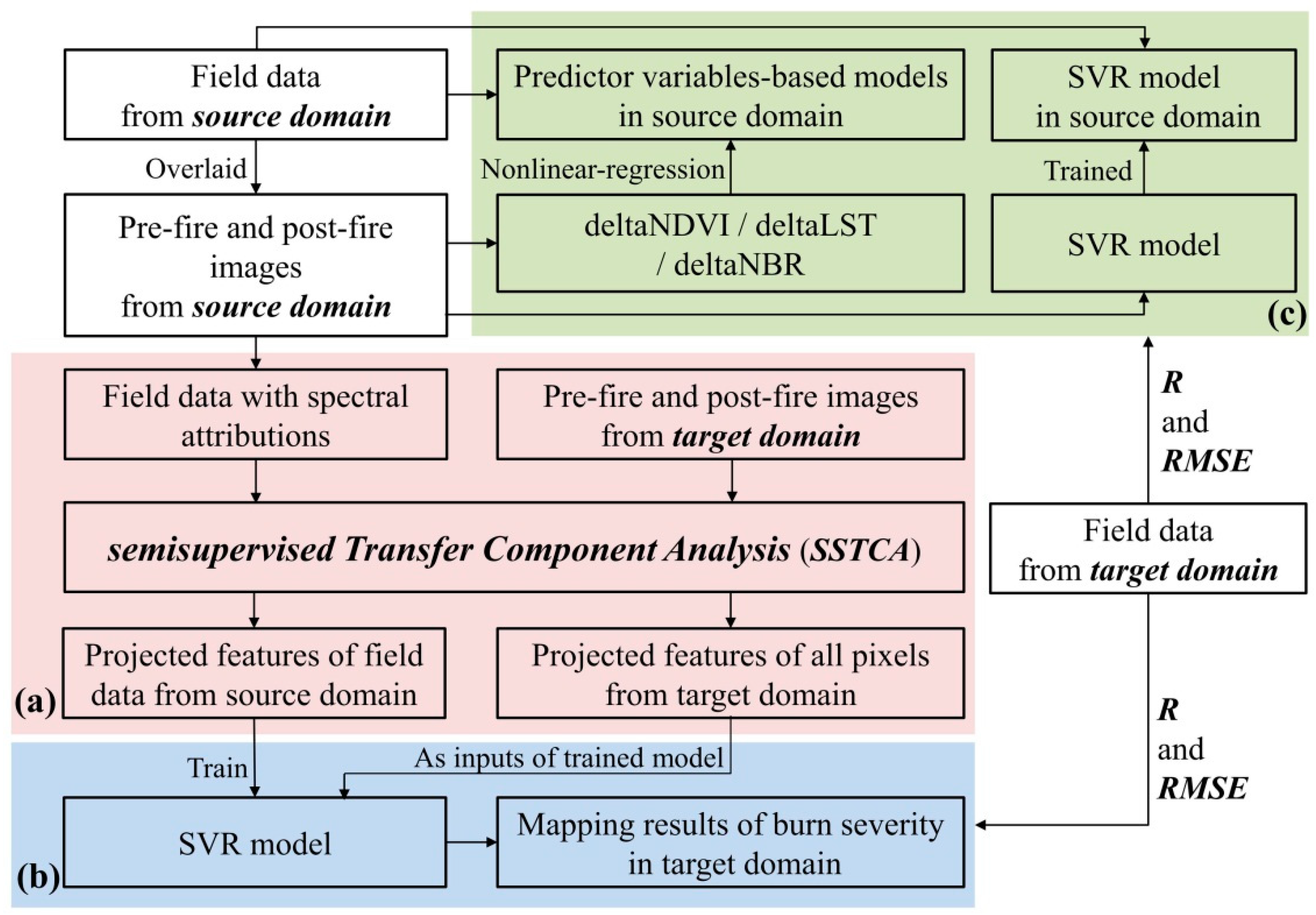
The SSTCA-SVR consists of the following three steps (see in Figure 1): (a) the SSTCA was applied at first to project a set of shared and invariant features from source and target domains [39]. (b) Based on the projected features of field survey data from source domain areas, support vector regression (SVR) model was trained and the burn severity level of each pixel from the target domain area was estimated. (c) The performance of SSTCA-SVR was validated and compared with that of other models (i.e., predictor variables-based regression models and SVR model with original spectral features). Its main operations are described in the following sections.
2.1. Domain Adaptation
Generally, a model for burn severity mapping is trained and applied in the same burned area, which means that training data and targeting data all come from the same domain area. Thus, the feature of these data should have the same distribution:
where XTr represents the feature space {xTr1, xTr2, ……, xTrn} of training data, YTr is their corresponding output which could be obtained using the field survey, and P(X) means a marginal probability of feature distributions. While, XTa is the feature space {xTa1, xTa2, ……, xTan} of target data and YTa is their corresponding output which needs to be estimated.
The corresponding outputs of training data are typically difficult to obtain because of the resources required [40]. Thus, there is a strong desire to make the use of any related data (i.e., source data) [38]. However, the distributions of source data and target data vary, since these data are collected under different background conditions:
where XS is the feature space {xS1, xS2, ……, xSn} of source data and YS are their corresponding outputs which have already been obtained in previous field survey.
Here, a transformation Φ is needed to project original spectral features of source and target data to an invariant subspace which can be shared:
This means that the distributions of source and target data are similar:
Hence, the model which was trained on projected features of source data could be applied to estimate corresponding outputs of target data with projected subspace feature as inputs. Next, the key issue is to find an appropriate transformation Φ using the SSTCA, which could be defined using a supervision process [38]. The resulting function of SSTCA should fulfill the following three objectives:
Objective 1: To minimize the distance between the distributions of Φ(XS) and Φ(XTa) in subspace after using the transformation Φ, as well as to preserve the variances of initial data.
The similarity of projected features in subspace should be great, which could be measured using a distance metric: Maximum Mean Discrepancy (i.e., Formula (A1) in Appendix A). By virtue of well-known kernel matrix (i.e., Formula (A2) in Appendix A) and coefficient L (i.e., Formula (A3)) in Appendix A), this distance can be written as a matrix trace (i.e., Formula (A4) in Appendix A). Further, considering the use of original kernel matrix K and transformation matrix W, kernel matrix between projected data (K*) could be calculated as Formula (A5) in Appendix A. Consequently, we could rewrite the Maximum Mean Discrepancy of projected source (XS*) and projected target (XTa*) data as Formula (A6) in Appendix A.
Meanwhile, the statistical properties of original data should be preserved, since it might be useful for the target supervised learning job. The variance matrix of projected samples (Σ*) could be quantitatively calculated as Formula (A7) in Appendix A.
Based on Objective 1, the unsupervised version of SSTCA (i.e., TCA) could be expressed as:
where is a regularization term which is introduced for controlling the complexity of W by adjusting μ.
Objective 2: To maximize the dependence between projected features of source data and their corresponding outputs. This is to make full use of outputs of available source data for defining an appropriate transformation Φ. Specifically, this objective could be expressed as:
where can be calculated as Formula (A9) in Appendix A.
Objective 3: To preserve the local geometrical structure. This is to ensure that close data in the original spectral feature space still are close in the projected subspace. This objective could be expressed as:
where is the graph Laplacian matrix which can be computed as Formula (A10) in Appendix A.
Integrated with Objective 2 and Objective 3, the Objective 1-based TCA can be updated as a semi-supervised version, i.e., the SSTCA:
The Formula (8) could be further reformulated as trace maximization which could be solved by introducing Lagrange multipliers and a supervision process. The SSTCA was implemented in this study using “a domain adaptation toolbox” of Matlab 2011b [41] and the Eigendecompose matrix is Formula (A12) in Appendix A. In this matrix, m leading eigenvectors is selected to build the matrix W for transformation Φ.
2.2. Burn Severity Mapping
After applying the transformation Φ, original spectral features of source data are projected to a shared subspace. Then, parameters of traditional SVR (i.e., ) are trained on these projected features (i.e., ) [42,43,44]. The basic principle of SVR model could be seen in Formula (A13) in Appendix A, which was executed in this study using the LIBSVM Toolbox of Matlab 2011b.
Based on the trained SVR model (i.e., ), could be replaced by the projected features of target data (i.e., ), since they distribute similarly in the projected subspace:
2.3. Performance Validation and Comparisons
Subsequently, a validation procedure was conducted to test the performance of SSTCA-SVR. More specifically, for field survey data from the target domain area, their estimated values were calculated using SSTCA-SVR and two accuracy measurements of R and RMSE were then computed. The performance of SSTCA-SVR was then evaluated against some predictor variables-based regression models (i.e., ∆NDVI, ∆LST, and ∆NBR) as well as that of SVR model with original spectral features.
3. Data and Processing
3.1. Study Area
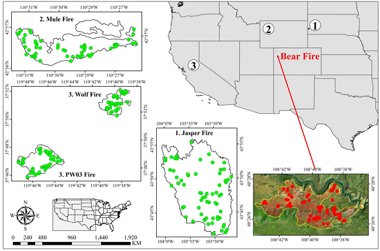
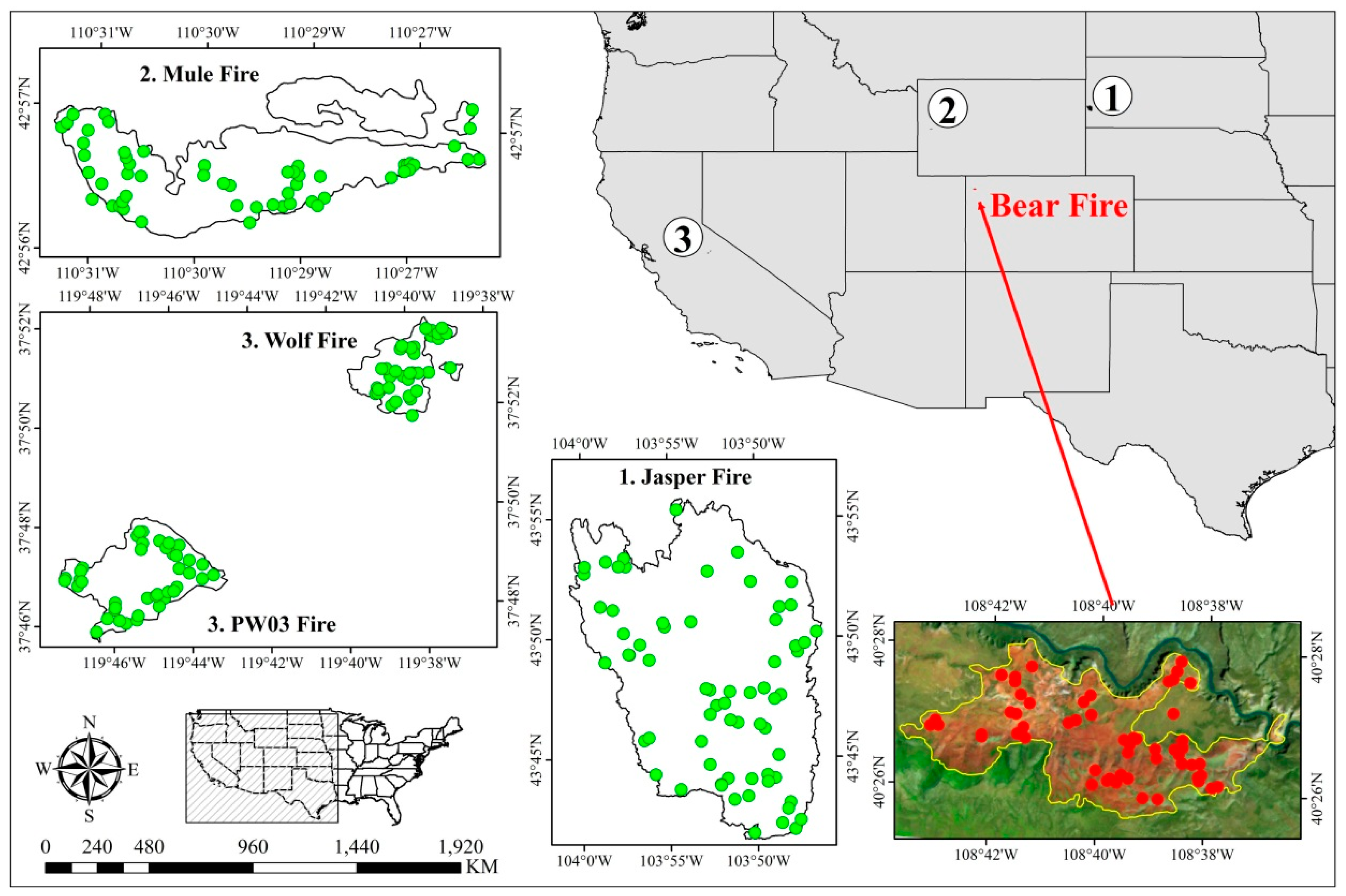
The Bear Fire, located in the Southwest of United States, was selected as the target domain area in this study (see in Figure 2). This fire occurred at the Dinosaur National Monument on 27 June 2002. After 8 days of burning, the final burned area was about 18.62 km2. This area was situated in the Highland (alpine) region with a low annual precipitation (<300 mm), which was mainly covered by trees, shrubs, and grasses.
Jasper Fire, Mule Fire, and PW03-Wolf Fire were chosen as the source domain areas where training data were from. The Jasper Fire, alarmed on 24 August 2000, was located in the Black Hills National Forest. Its burned area was about 336 km2. The local region was Semiarid Steppe climate and the primary tree species was ponderosa pine. The Mule Fire was caused by lightning strike on 11 July 2002 and occurred in Northern Rockies region. Its climate also belongs to Highland (alpine) with annual precipitation between 750 and 1150 mm. Predominant tree species in this area were subalpine fir, Engelmann spruce, and Douglas-fir. The Pw03-Wolf Fire includes two nearby fires and both of them were located in the Yosemite National Park of California region. These burned area featured Mediterranean climate with a high annual precipitation being between 804 and 1722 mm. The Chaparral and Sierra Mixed Conifer were primary vegetation species in this area. More descriptions about abovementioned fires could be found in reported studies [8,30,45].
3.2. Remotely Sensed Data
Three sets of remotely sensed data (i.e., Landsat 5 TM, Landsat 7 ETM+, and Terra MODIS) were obtained in this study (see in Table 1). For each fire, TM or ETM+ satellite images, close to the collection time of field survey data, were selected as post-fire remotely sensed data. The pre-fire remotely sensed data were selected according to the principle of “minimal moisture contents and phenology difference.” All TM and ETM+ remotely sensed data were downloaded from the U.S. Geological Survey EarthExplorer, which have already undergone Level L1G processing [46]. Subsequently, reflectance transformation and atmospheric correction were done with the ENVI 5.0 software.
To calculate LST for each fire, one MODIS product (i.e., total precipitable water, MOD05_L2. v051) was employed as atmospheric water vapor content for application of generalized single-channel algorithm. At first, this product was georeferenced using the MODIS Conversion Toolkit tool of ENVI 5.0 software. It was then resampled for matching the spatial resolution of thermal infrared band. A second MODIS product (i.e., Daily Land Surface Temperature/Emissivity, MOD11A1.v005) was applied to check the rightness of Landsat-based LST calculations [30,47]. All these MODIS data were obtained from the NASA’s Level 1 and Atmosphere Archive and Distribution System (LAADS Web) [48].
3.3. Field Survey Data
The CBI field survey data were collected during the first or second following growing season for extended assessment for each fire [7]. All field survey data were obtained from the Joint Fire Science Program (JFSP) project which was undertaken by National Park Service and the US Geological Survey [45]. The specific number of field survey data for each fire is: 55 for Bear Fire, 66 for Jasper Fire, 55 for Mule Fire, and 78 for Pw03-Wolf Fire. Based on the recorded locations during data collections, each CBI field survey data was matched with corresponding pixel on remote sensing images. In a 3 × 3 matrix centered on matched pixel, the spectral value of each band was extracted and averaged to reduce the influence of GPS positioning error [30].
3.4. Cross-Validation Setting
First, the Bear Fire was selected as the target domain area and all CBI field survey data were employed as testing data to validate the accuracy of mapping results of burn severity. Meanwhile, Jasper, Mule, and PW03-Wolf Fire were chosen as the source domain areas. This means all CBI field survey data in these fires were applied to train predictor variables-based regression, SVR, and SSTCA-SVR models. Then, to further evaluate the performance of SSTCA-SVR in different eco-type regions, a cross-validation procedure was repeated by sequentially changing the target domain area and the source domain areas. Four scenarios were finally formed as follows (see in Table 2).
4. Results
4.1. Parameters Analysis of SSTCA
The SSTCA was applied in this study as domain adaptation approach to project original spectral features of target and source data. As described in Section 2, it mainly involved six parameters, i.e., μ, γ, kernel function, k, number of projected features, and λ. Specifically, μ was used for adjusting the complexity of transformation matrix in Formula (5) and γ was employed to balance the outputs dependence and the data variance in Formula (A9) in Appendix A. They were respectively fixed to 1 and 0.5 based on the preliminary tests and some reported researches [38,39]. Meanwhile, several preliminary trials suggested that the kernel function in Formula (A2) in Appendix A should be set to “Linear” and the optimum number of k neighbors in Formula (A11) in Appendix A was 100 which was also consistent with the previous research [39]. Therefore, only two parameters (i.e., number of projected features and λ) need to be further fitted for SSTCA in this study.
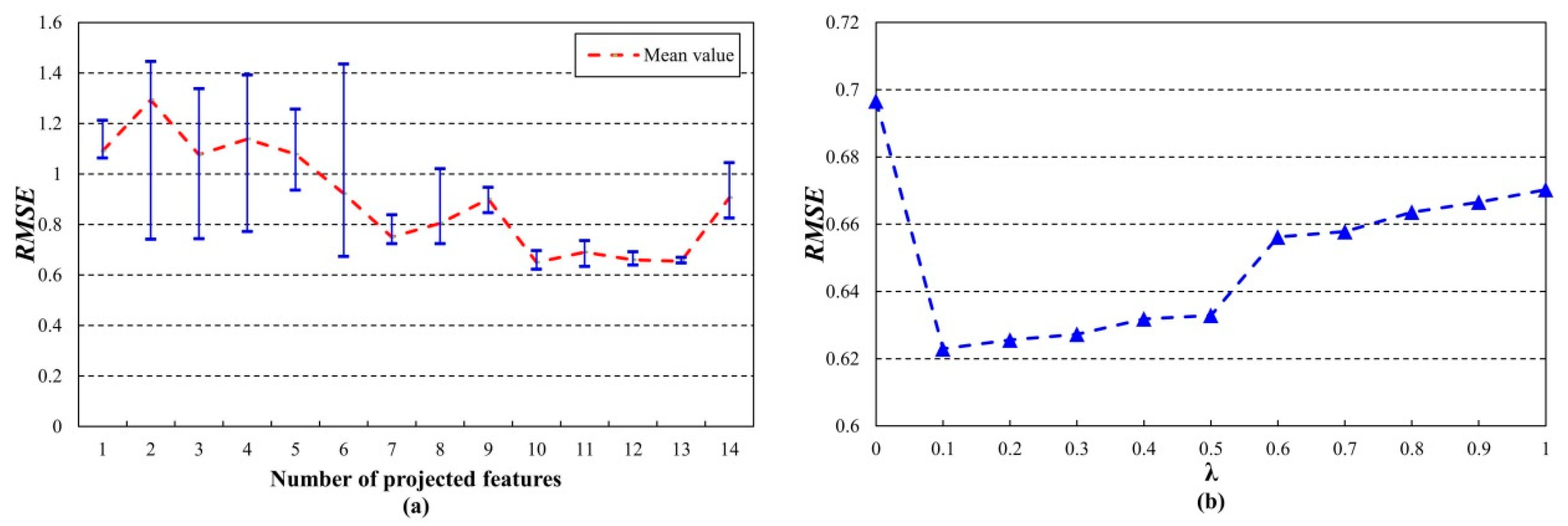
Figure 3a shows that, when the number of projected features varied from 1 to 14, mean RMSE value decreased and then increased. The minimum RMSE value was 0.6229, when the number of projected features was 10. Thus, the optimum number of projected features on Bear Fire should be 10. After this setting, Figure 3b further displays that optimal value of parameter λ should be 0.1, when it was chosen between 0 and 1. At last, optimal parameters (i.e., μ = 1, γ = 0.5, kernel = linear, k = 100, number of projected features = 10, and λ = 0.1) were fixed in SSTCA for projecting the original spectral features of source domain areas (i.e., Jasper, Mule, and PW-03 Fire) and the target domain area (i.e., Bear Fire) to an invariant and shared subspace.
4.2. Visual Analysis of Projected Features
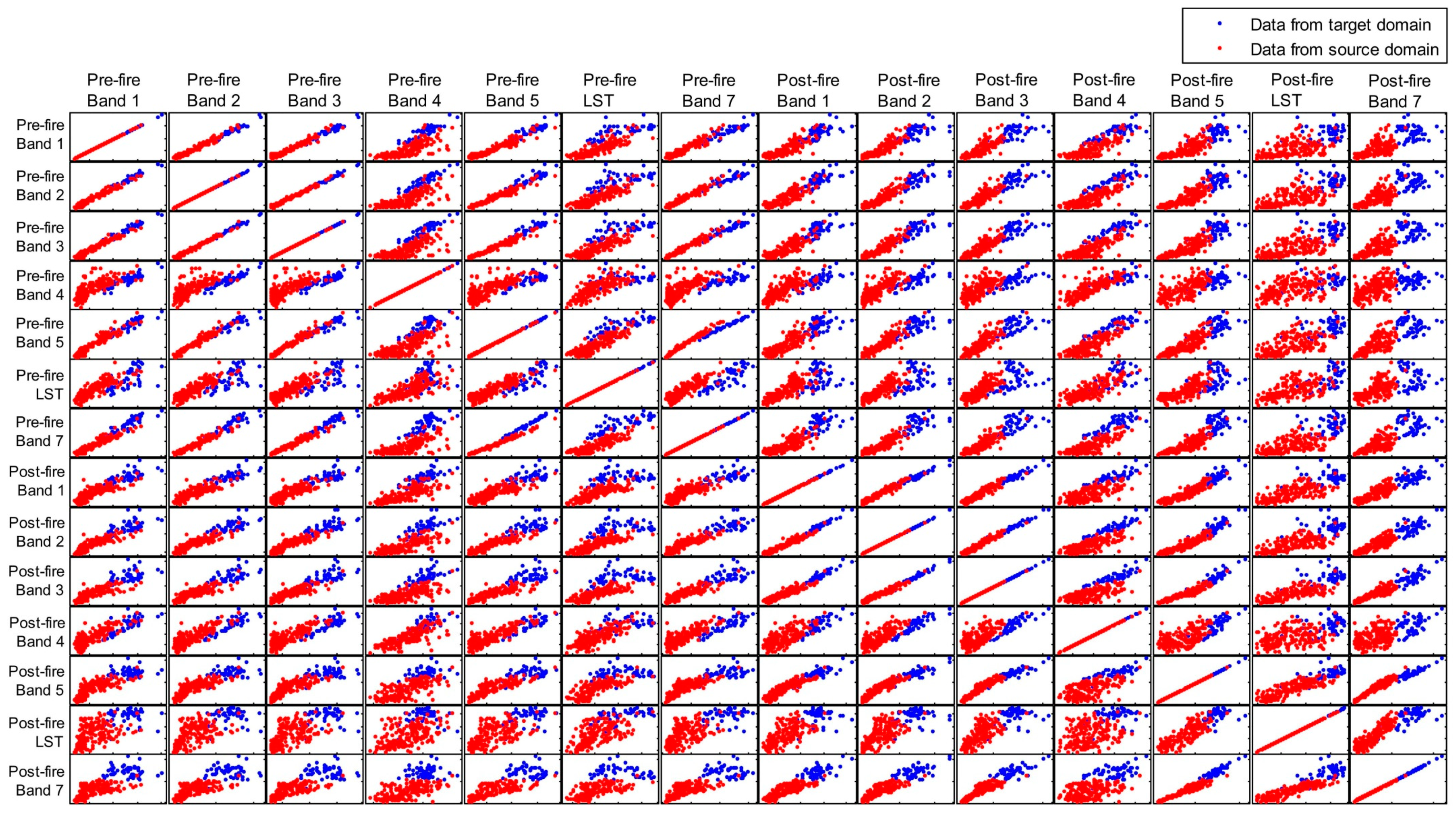
Across the target domain area (i.e., blue dots) and source domain areas (i.e., red dots), original spectral feature space of remote sensing data (i.e., spectral bands of pre- and post-fire images) was plotted. Figure 4 illustrates that, in most scatter plots, blue and red dots have different distributions. This means that a difference of each band in original spectral feature space was evident.
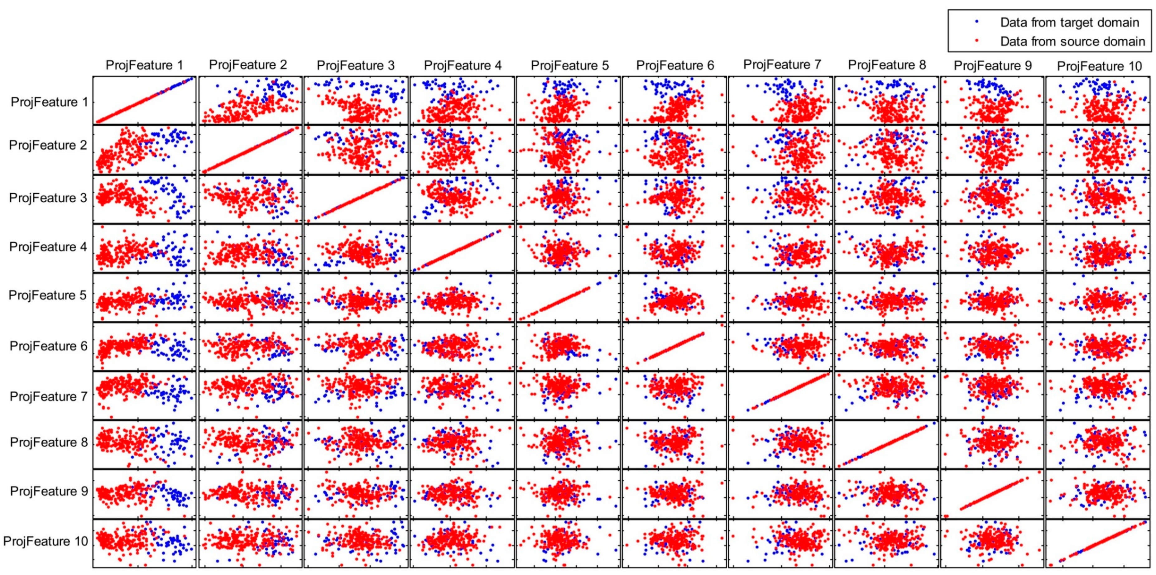
Based on the optimal parameters selected in Section 4.1, ten projected features were transformed using SSTCA. Figure 5 shows that the distributions of blue dots were similar with that of red dots in most scatter plots. This means that, in these projected feature spaces, the model trained from data of source domain areas could be transferred to data of the target domain area. Figure 5 also displays that, after domain adaptation of SSTCA, data from source and target domain areas have the maximum variance, which means that transformation matrix of the fixed SSTCA have fulfilled the objective 1 in Section 2 (i.e., preserving the variances of initial data in Formula (7)). This maximized variance of data would be very useful for following supervised learning job.
4.3. Mapping Results of Burn Severity
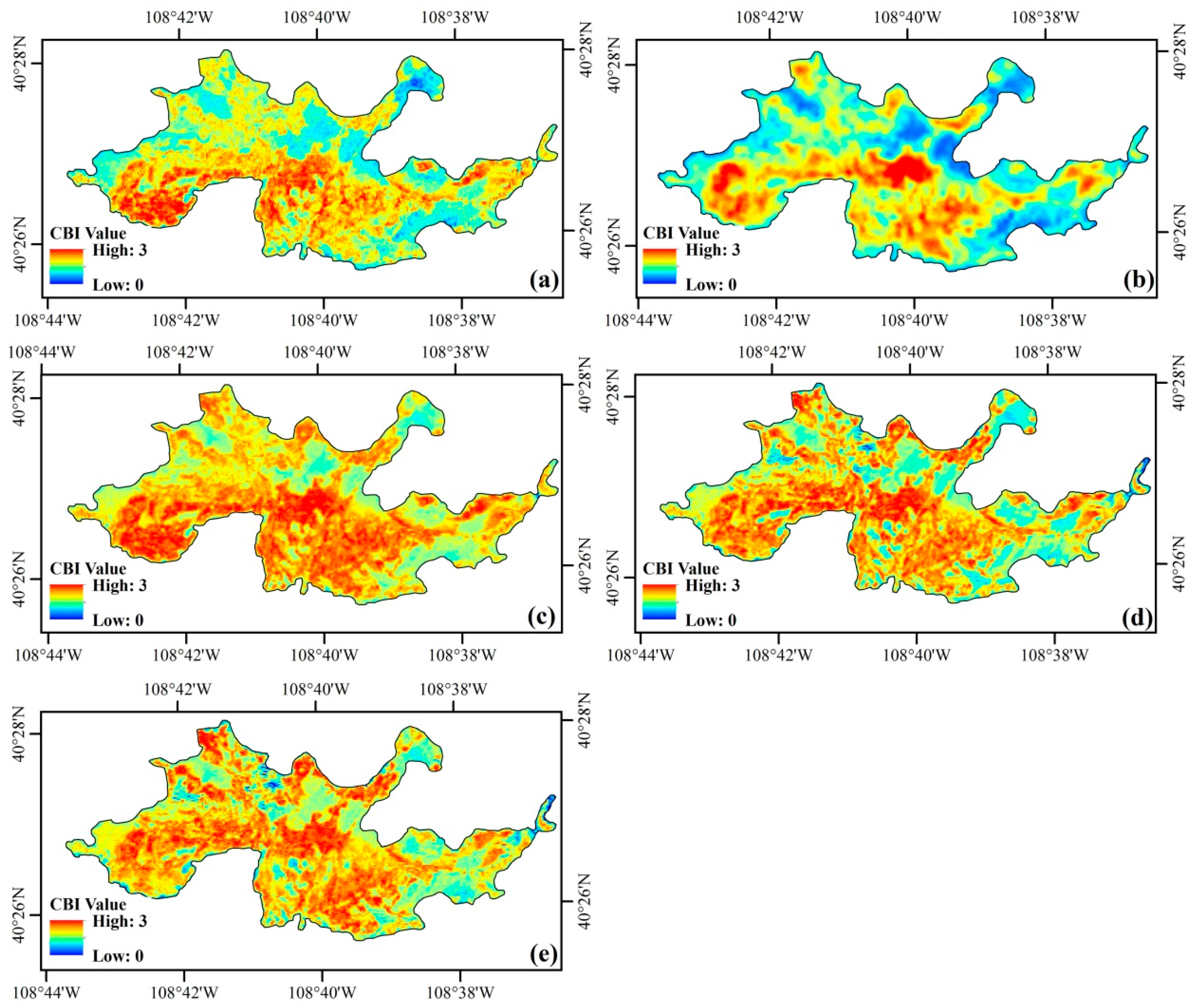
As a specific example, mapped results of burn severity across Bear Fire were chosen for analysis. From a visual perspective, Figure 6 exhibits that the spatial distributions of burn severity mapped by using different methods were similar as a whole. However, the mapped spatial distribution of CBI value using ∆LST-based model was coarser as shown in Figure 6b. This was because LST value was calculated from thermal infrared data of Landsat TM/ETM+ which has a lower spatial resolution (i.e., 60 m/120 m). In contrast, it can be observed from Figure 6 that spatial distributions of burn severity mapped by SSTCA-SVR were finer than that of other predictor variables-based empirical fitting models. Although SVR model also has a fine burn severity results, its values were generally higher than that of SSTCA-SVR.
From a quantitative perspective, the field survey data of Bear Fire were employed as testing data to validate the accuracy of mapped results in Figure 6. Statistical results of accuracy in Table 3 revealed that SSTCA-SVR has the best performance at mapping burn severity with the lowest error value (i.e., RMSE is 0.6229). In contrast, we found that mapping result of SVR has the lowest accuracy with the highest RMSE value of 1.7658. This was consistent with the visual analysis result shown in Figure 6. The RMSE values of other predictor variables-based regression models were between 0.7362 and 1.1187.
4.4. Cross-Validation in Different Scenarios
In order to further verify the reliability of SSTCA-SVR model in different eco-type regions, a cross-validation has been applied to sequentially exchange target and source domain data. Similar procedures in Section 4.1, Section 4.2 and Section 4.3 were operated in each scenario. Table 4 illustrates that SSTCA-SVR has the best performance at mapping burn severity in all scenarios (RMSE values are between 0.4833 and 0.6659). On the contrary, accuracies of mapped results by using SVR were the worst (RMSE value varies from 1.7658 to 2.0055), which was consistent with the above results in Figure 6 and Table 3. Moreover, ∆NBR-based regression model has a similar performance (i.e., RMSE value is 0.5917) with SSTCA-SVR (i.e., RMSE value is 0.5824) in Scenario 4.
5. Discussion
In this study, a transfer learning-based model was developed to map the burn severity of forest fire. Our findings suggest that, based on the domain adaptation of SSTCA approach, the proposed model could transfer knowledge from other burned areas. This model will be very helpful for mapping severity levels across burned areas where field survey data are not available. This research has advanced our capability to use remotely sensed data to quantitatively measure the damage levels after forest fire.
In original spectral features space, the data distributions of source and target domain areas indeed are different, since the remotely sensed data with temporal and spatial variations have different spectral signature. Thus, models which were trained on data from source domain areas should not be directly applied to map burn severity of a target domain area. This might result in a poor performance, which has been confirmed in experimental results.
Experimental results further indicated that, using SSTCA approach, original spectral features of target and source domains can be projected to a new subspace. In this subspace, data distributions of source and target domains actually are similar, which means that trained knowledge from source domain areas could be transferred to the target domain area. This fact also has been verified by subsequent experimental results. Therefore, to build a model for mapping burn severity of burned areas without field survey data, the domain adaptation is needed at first.
Moreover, results in this study have revealed that some predictor variables-based regression models (i.e., ∆NDVI, ∆LST, and ∆NBR) also have a certain transferring ability across target and source domain areas. This result agrees with that of a reported study [37], in which the overall ∆NBR-derived model has the transferability across multiple western Canadian landscapes. For spectral indices (e.g., NDVI and NBR), their calculations mainly are based on the differencing and ratio operations of spectral bands. This can reduce spectral changing of each original band caused by environmental variations to a certain extent. As for LST, it was retrieved in this study using the generalized single-channel algorithm from the radiative transfer equation [49,50]. During its retrieval process, variations of local environmental factors (e.g., atmospheric water vapor content, vegetation cover, and land surface emissivity) have also been considered as inputs of retrieval algorithm. Therefore, LST variations caused by environmental variations have been reduced and the transferring ability of LST-based model can also be observed across different domain areas.
In essence, the domain adaptation in the proposed model performs a similar function as the calculation of predictor variables (i.e., ∆NDVI, ∆LST, and ∆NBR), since they all have extracted several new features from original spectral features space. However, the calculation of predictor variables was based on limited spectral bands, which would lead to a lower transferring ability. In contrast, SSTCA method has projected all original spectral bands to exclude the difference of spectral signature. This means that more spectral information as possible have been utilized to map burn severity. Therefore, SSTCA-SVR model could map the burn severity finer and its obtained results have higher accuracy [8].
Compared to the LST-based model, SSTCA-SVR model not only has higher accuracy, but also higher efficiency. The reason for this is that SSTCA-SVR could be considered one type of machine learning algorithms, in which all model parameters could be learned by using supervision process and optimization procedure. Therefore, SSTCA-SVR model is relatively simple and efficient without setting of complex physical parameters and supporting of external environmental data.
Lastly, this research has introduced a potentially efficient mechanism to map burn severity, which could speed up the response of post-fire management. Unlike traditional mapping process which requires field survey data to build the regression model, only remote sensing data in the target domain area and field survey data in the source domain areas are needed as inputs of SSTCA-SVR. This means that burn severity levels can be mapped quickly with a certain degree of reliability, as long as appropriate remote sensing data are obtained across target burned areas. There is no need to wait for the collection of field survey data and external support data.
We should acknowledge that the transferring ability of SSTCA-SVR is limited, when climatic variations between source domain area (e.g., Pw03-Wolf Fire is located in the Mediterranean climate region) and target domain areas (e.g., Bear, Jasper, and Mule Fires are located in the Highland and Semiarid Steppe climate regions) are very high. It thus can be found in Scenario 4 that the accuracy of SSTCA-SVR is similar with that of ∆NBR-based regression model. But, for a specific target domain area (e.g., in African savanna), this limitation could be overcome to a certain extent if some historical field survey data in the similar climate region are available.
Moreover, considering the availability of CBI-field survey data, the performance of SSTCA-SVR was only tested in the Midwestern United States. Its transferring ability needs to be further validated in different types of forest ecosystems around the world. Subsequent studies also are required to explore the spatial scale adaptability of SSTCA-SVR across different geographic regions in the future.
6. Conclusions
In this study, a transfer learning-based model was proposed to map the severity levels across the burned areas without field survey data. We have evaluated the performance of proposed model in different eco-type regions of Southwestern United States. Results indicate that original spectral features with different characteristic could be projected to an invariant and shared subspace by using SSTCA approach. Based on these projected features, the SVR model which was trained on source domain areas could be transferred to a target domain area. Compared to that of ∆NDVI-, ∆LST-, ∆NBR-, and SVR-based models, mapped results of CBI values using by SSTCA-SVR were more fine and accurate. This research has further developed our capability to use remotely sensed data to map the burn severity of forest fire. Moreover, this study has introduced a potentially efficient mechanism to map the burn severity to speed up the response of post-fire management.
Author Contributions
Z.Z. performed the experiment designing, the data analysis, as well as the manuscript writing; J.W. supervised the research work; B.S. helped with revisions. All authors contributed to writing the paper. All authors have read and agreed to the published version of the manuscript.
Funding
This work has been funded by the National Natural Science Foundation of China under Grant number 41801315, 41771535, the program of China Scholarship Council under Grant number 201908510029, the Open Research Fund of Chongqing Meteorological Bureau under Grant number KFJJ-201705, the Project Supported by the Scientific Research Foundation of CUIT under Grant number KYTZ201742, and the Scientific Research Foundation of the Education Department of Sichuan Province under Grant number 18ZB0128.
Acknowledgments
The authors would like to acknowledge the data made available by the U.S. Geological Survey, the U.S. Geological Survey’s National Center for Earth Resources Observation and Science, the USDA Forest Service Remote Sensing Applications Center for making remote sensing data available, and the Joint Fire Science Program (JFSP) project undertaken by the National Park Service and the US Geological Survey. We wish to thank the editor and anonymous reviewers for their thoughtful and helpful comments.
Conflicts of Interest
The authors declare no conflict of interest.
Appendix A
While, is the identify matrix () and 1 is the column vector with all 1′s ().
where is to maximize the outputs dependence and maximize the data variance. The is used as the tradeoff parameter to balance the two terms.
where D is a diagonal matrix with elements and the Mi,j can be calculated as:
where represents the model complexity, slack variables (, ) are deviation measurements, and tradeoff constant C determines tradeoff between these two terms.
References
- Dixon, R.K.; Solomon, A.M.; Brown, S.; Houghton, R.A.; Trexier, M.C.; Wisniewski, J. Carbon pools and flux of global forest ecosystems. Science 1994, 263, 185–190. [Google Scholar] [CrossRef] [PubMed]
- Park, H.-J.; Lim, S.-S.; Yang, H.I.; Lee, K.-S.; Park, S.-I.; Kwak, J.-H.; Kim, H.-Y.; Oh, S.-W.; Choi, W.-J. Co-elevated CO2 and temperature and changed water availability do not change litter quantity and quality of pine and oak. Agric. For. Meteorol. 2020, 280, 107795. [Google Scholar] [CrossRef]
- Zheng, Z.; Huang, W.; Li, S.; Zeng, Y. Forest fire spread simulating model using cellular automaton with extreme learning machine. Ecol. Model. 2017, 348, 33–43. [Google Scholar] [CrossRef] [Green Version]
- Quintano, C.; Fernandez-Manso, A.; Roberts, D.A. Burn severity mapping from landsat mesma fraction images and land surface temperature. Remote Sens. Environ. 2017, 190, 83–95. [Google Scholar] [CrossRef]
- Chen, G.; Metz, M.R.; Rizzo, D.M.; Dillon, W.W.; Meentemeyer, R.K. Object-based assessment of burn severity in diseased forests using high-spatial and high-spectral resolution master airborne imagery. ISPRS J. Photogramm. Remote Sens. 2015, 102, 38–47. [Google Scholar] [CrossRef] [Green Version]
- Chuvieco, E.; Riaño, D.; Danson, F.M.; Martin, P. Use of a radiative transfer model to simulate the postfire spectral response to burn severity. J. Geophys. Res. Biogeosci. 2006, 111. [Google Scholar] [CrossRef] [Green Version]
- Key, C.H.; Benson, N.C. Landscape assessment (la): Sampling and analysis methods. In Rocky Mountain Research Station, USDA; Forest Service: Fort Collins, CO, USA, 2006; pp. LA-1–LA-51. [Google Scholar]
- Zheng, Z.; Zeng, Y.; Li, S.; Huang, W. Mapping burn severity of forest fires in small sample size scenarios. Forests 2018, 9, 608. [Google Scholar] [CrossRef] [Green Version]
- Schepers, L.; Haest, B.; Veraverbeke, S.; Spanhove, T.; Vanden Borre, J.; Goossens, R. Burned area detection and burn severity assessment of a heathland fire in belgium using airborne imaging spectroscopy (apex). Remote Sens. 2014, 6, 1803–1826. [Google Scholar] [CrossRef] [Green Version]
- He, Y.; Chen, G.; De Santis, A.; Roberts, D.A.; Zhou, Y.; Meentemeyer, R.K. A disturbance weighting analysis model (dwam) for mapping wildfire burn severity in the presence of forest disease. Remote Sens. Environ. 2019, 221, 108–121. [Google Scholar] [CrossRef]
- Quintano, C.; Fernández-Manso, A.; Roberts, D.A. Multiple endmember spectral mixture analysis (mesma) to map burn severity levels from landsat images in mediterranean countries. Remote Sens. Environ. 2013, 136, 76–88. [Google Scholar] [CrossRef]
- De Santis, A.; Chuvieco, E.; Vaughan, P.J. Short-term assessment of burn severity using the inversion of prospect and geosail models. Remote Sens. Environ. 2009, 113, 126–136. [Google Scholar] [CrossRef]
- De Santis, A.; Chuvieco, E. Burn severity estimation from remotely sensed data: Performance of simulation versus empirical models. Remote Sens. Environ. 2007, 108, 422–435. [Google Scholar] [CrossRef]
- Epting, J.; Verbyla, D.; Sorbel, B. Evaluation of remotely sensed indices for assessing burn severity in interior alaska using landsat tm and etm+. Remote Sens. Environ. 2005, 96, 328–339. [Google Scholar] [CrossRef]
- Veraverbeke, S.; Hook, S.; Hulley, G. An alternative spectral index for rapid fire severity assessments. Remote Sens. Environ. 2012, 123, 72–80. [Google Scholar] [CrossRef]
- van Wagtendonk, J.W.; Root, R.R.; Key, C.H. Comparison of aviris and landsat etm+ detection capabilities for burn severity. Remote Sens. Environ. 2004, 92, 397–408. [Google Scholar] [CrossRef]
- Key, C.H.; Benson, N.C. The Normalized Burn Ratio (nbr): A Landsat tm Radiometric Measure of Burn Severity. Available online: http://www.nrmsc.usgs.gov/research/ndbr.htm (accessed on 22 May 2015).
- Garcia, M.L.; Caselles, V. Mapping burns and natural reforestation using thematic mapper data. Geocarto Int. 1991, 6, 31–37. [Google Scholar] [CrossRef]
- Cocke, A.E.; Fulé, P.Z.; Crouse, J.E. Comparison of burn severity assessments using differenced normalized burn ratio and ground data. Int. J. Wildland Fire 2005, 14, 189–198. [Google Scholar] [CrossRef] [Green Version]
- Roy, D.P.; Boschetti, L.; Trigg, S.N. Remote sensing of fire severity: Assessing the performance of the normalized burn ratio. IEEE Geosci. Remote Sens. Lett. 2006, 3, 112–116. [Google Scholar] [CrossRef] [Green Version]
- Escuin, S.; Navarro, R.; Fernandez, P. Fire severity assessment by using nbr (normalized burn ratio) and ndvi (normalized difference vegetation index) derived from landsat tm/etm images. Int. J. Remote Sens. 2008, 29, 1053–1073. [Google Scholar] [CrossRef]
- Zheng, Z. Study on the risk, spread and assessment of forest fire based on the model and remote sensing. Acta Geod. Cartogr. Sin. 2019, 48, 133. [Google Scholar]
- Soverel, N.O.; Perrakis, D.D.B.; Coops, N.C. Estimating burn severity from landsat dnbr and rdnbr indices across western canada. Remote Sens. Environ. 2010, 114, 1896–1909. [Google Scholar] [CrossRef]
- Miller, J.D.; Thode, A.E. Quantifying burn severity in a heterogeneous landscape with a relative version of the delta normalized burn ratio (dnbr). Remote Sens. Environ. 2007, 109, 66–80. [Google Scholar] [CrossRef]
- Heward, H.; Smith, A.M.S.; Roy, D.P.; Tinkham, W.T.; Hoffman, C.M.; Morgan, P.; Lannom, K.O. Is burn severity related to fire intensity? Observations from landscape scale remote sensing. Int. J. Wildland Fire 2013, 22, 910–918. [Google Scholar] [CrossRef]
- Parks, S.; Dillon, G.; Miller, C. A new metric for quantifying burn severity: The relativized burn ratio. Remote Sens. 2014, 6, 1827–1844. [Google Scholar] [CrossRef] [Green Version]
- Lentile, L.B.; Holden, Z.A.; Smith, A.M.S.; Falkowski, M.J.; Hudak, A.T.; Morgan, P.; Lewis, S.A.; Gessler, P.E.; Benson, N.C. Remote sensing techniques to assess active fire characteristics and post-fire effects. Int. J. Wildland Fire 2006, 15, 319–345. [Google Scholar] [CrossRef]
- Quintano, C.; Fernández-Manso, A.; Calvo, L.; Marcos, E.; Valbuena, L. Land surface temperature as potential indicator of burn severity in forest mediterranean ecosystems. Int. J. Appl. Earth Obs. Geoinf. 2015, 36, 1–12. [Google Scholar] [CrossRef]
- Fernández-García, V.; Santamarta, M.; Fernández-Manso, A.; Quintano, C.; Marcos, E.; Calvo, L. Burn severity metrics in fire-prone pine ecosystems along a climatic gradient using landsat imagery. Remote Sens. Environ. 2018, 206, 205–217. [Google Scholar] [CrossRef]
- Zheng, Z.; Zeng, Y.; Li, S.; Huang, W. A new burn severity index based on land surface temperature and enhanced vegetation index. Int. J. Appl. Earth Obs. Geoinf. 2016, 45, 84–94. [Google Scholar] [CrossRef]
- Veraverbeke, S.; Verstraeten, W.W.; Lhermitte, S.; Van De Kerchove, R.; Goossens, R. Assessment of post-fire changes in land surface temperature and surface albedo, and their relation with fire–burn severity using multitemporal modis imagery. Int. J. Wildland Fire 2012, 21, 243–256. [Google Scholar] [CrossRef] [Green Version]
- Marcos, E.; Fernández-García, V.; Fernández-Manso, A.; Quintano, C.; Valbuena, L.; Tárrega, R.; Luis-Calabuig, E.; Calvo, L. Evaluation of composite burn index and land surface temperature for assessing soil burn severity in mediterranean fire-prone pine ecosystems. Forests 2018, 9, 494. [Google Scholar] [CrossRef] [Green Version]
- Harris, S.; Veraverbeke, S.; Hook, S. Evaluating spectral indices for assessing fire severity in chaparral ecosystems (southern california) using modis/aster (master) airborne simulator data. Remote Sens. 2011, 3, 2403–2419. [Google Scholar] [CrossRef] [Green Version]
- Vlassova, L.; Pérez-Cabello, F.; Mimbrero, M.; Llovería, R.; García-Martín, A. Analysis of the relationship between land surface temperature and wildfire severity in a series of landsat images. Remote Sens. 2014, 6, 6136–6162. [Google Scholar] [CrossRef] [Green Version]
- Chen, G.; Metz, M.R.; Rizzo, D.M.; Meentemeyer, R.K. Mapping burn severity in a disease-impacted forest landscape using landsat and master imagery. Int. J. Appl. Earth Obs. Geoinf. 2015, 40, 91–99. [Google Scholar] [CrossRef] [Green Version]
- Fernández-Manso, O.; Quintano, C.; Fernández-Manso, A. Combining spectral mixture analysis and object-based classification for fire severity mapping. For. Syst. 2009, 18, 296–313. [Google Scholar] [CrossRef]
- Soverel, N.O.; Coops, N.C.; Perrakis, D.D.B.; Daniels, L.D.; Gergel, S.E. The transferability of a dnbr-derived model to predict burn severity across 10 wildland fires in western canada. Int. J. Wildland Fire 2011, 20, 518–531. [Google Scholar] [CrossRef]
- Pan, S.J.; Tsang, I.W.; Kwok, J.T.; Yang, Q. Domain adaptation via transfer component analysis. IEEE Trans. Neural Netw. 2011, 22, 199–210. [Google Scholar] [CrossRef] [Green Version]
- Matasci, G.; Volpi, M.; Kanevski, M.; Bruzzone, L.; Tuia, D. Semisupervised transfer component analysis for domain adaptation in remote sensing image classification. IEEE Trans. Geosci. Remote Sens. 2015, 53, 3550–3564. [Google Scholar] [CrossRef]
- Yan, K.; Kou, L.; Zhang, D. Learning domain-invariant subspace using domain features and independence maximization. IEEE Trans. Cybern. 2018, 48, 288–299. [Google Scholar] [CrossRef]
- Yan, K. A Domain Adaptation Toolbox. Available online: https://www.github.com/viggin/domain-adaptation-toolbox (accessed on 9 December 2019).
- Cherkassky, V.; Ma, Y. Practical selection of svm parameters and noise estimation for svm regression. Neural Netw. 2004, 17, 113–126. [Google Scholar] [CrossRef] [Green Version]
- Vapnik, V.N. An overview of statistical learning theory. IEEE Trans. Neural Netw. 1999, 10, 988–999. [Google Scholar] [CrossRef] [Green Version]
- Vapnik, V.N. Statistical Learning Theory; Wiley: New York, NY, USA, 1998; Volume 2. [Google Scholar]
- Zhu, Z.; Key, C.; Ohlen, D.; Benson, N.C. Evaluate sensitivities of burn-severity mapping algorithms for different ecosystems and fire histories in the united states. In Final Report to the Joint Fire Science Program; JFSP 01-1-4-12; Joint Fire Science Program: Boise, IA, USA, 2006. [Google Scholar]
- USGS. Earthexplorer. Available online: http://earthexplorer.usgs.gov/ (accessed on 20 December 2013).
- Srivastava, P.K.; Majumdar, T.J.; Bhattacharya, A.K. Surface temperature estimation in singhbhum shear zone of india using landsat-7 etm+ thermal infrared data. Adv. Space Res. 2009, 43, 1563–1574. [Google Scholar] [CrossRef]
- NASA. Level 1 and Atmosphere Archive and Distribution System (LAADS). Available online: http://earthexplorer.usgs.gov/ (accessed on 20 October 2014).
- Zhou, J.; Li, J.; Zhang, L.; Hu, D.; Zhan, W. Intercomparison of methods for estimating land surface temperature from a landsat-5 tm image in an arid region with low water vapour in the atmosphere. Int. J. Remote Sens. 2012, 33, 2582–2602. [Google Scholar] [CrossRef]
- Zhang, Z.; He, G.; Wang, M.; Long, T.; Wang, G.; Zhang, X. Validation of the generalized single-channel algorithm using landsat 8 imagery and surfrad ground measurements. Remote Sens. Lett. 2016, 7, 810–816. [Google Scholar] [CrossRef]
Figure 1.
The flowchart of methodology: (a) domain adaptation; (b) burn severity mapping; and (c) performance validation and comparisons.
Figure 1.
The flowchart of methodology: (a) domain adaptation; (b) burn severity mapping; and (c) performance validation and comparisons.

Figure 2.
The location of study area in the southwest of United States. Red plots are testing data from target domain area and Green plots are training data from source domain areas.
Figure 2.
The location of study area in the southwest of United States. Red plots are testing data from target domain area and Green plots are training data from source domain areas.

Figure 3.
Performance of SSTCA-SVR on Bear Fire with respect to two parameters: (a) the number of projected-features and (b) λ. Note that the SSTCA-SVR has the lowest RMSE value, with number of projected features set to 10. After this setting, the optimal value for λ was 0.1.
Figure 3.
Performance of SSTCA-SVR on Bear Fire with respect to two parameters: (a) the number of projected-features and (b) λ. Note that the SSTCA-SVR has the lowest RMSE value, with number of projected features set to 10. After this setting, the optimal value for λ was 0.1.

Figure 4.
The scatter plot matrix of original spectral feature space over Bear Fire. Each panel is one scatter plot of a pair of spectral bands. Blue dots are field survey data from the target domain area: Bear Fire (n = 55). Red dots are field survey data from source domain areas: Jasper, Mule, and PW03-Wolf Fires (n = 199). Note that the distributions of data from target domain area and source domain areas are different in original spectral feature spaces.

Figure 5.
The scatter plot matrix of projected feature spaces over Bear Fire. Each panel is one scatter plot of a pair of projected features. Blue dots are field survey data from the target domain area: Bear Fire (n = 55). Red dots are field survey data from source domain areas: Jasper, Mule, and PW03-Wolf Fires (n = 199). Note that the distributions of data from target domain area and source domain areas are similar in most projected feature spaces.

Figure 6.
Mapped results of burn severity levels across Bear Fire using different models: (a) ∆NDVI-based regression model; (b) ∆LST-based regression model; (c) ∆NBR-based regression model; (d) SVR model; and (e) SSTCA-SVR model.
Figure 6.
Mapped results of burn severity levels across Bear Fire using different models: (a) ∆NDVI-based regression model; (b) ∆LST-based regression model; (c) ∆NBR-based regression model; (d) SVR model; and (e) SSTCA-SVR model.


Table 1.
Summary of study area and data.
| Fire Name | Bear | Jasper | Mule | Pw03-Wolf |
|---|---|---|---|---|
| Regional Eco-types | Southwest | Central | Northern Rockies | California |
| Alarmed Date | 27 June 2002 | 24 August 2000 | 11 July 2002 | 3 October 2002 and 11 July 2002 |
| Regional Climate | Highland (alpine) | Semiarid Steppe | Highland (alpine) | Mediterranean |
| Annual Precipitation | <300 mm | 440 to 673 mm | 750 to 1150 mm | 804 to 1722 mm |
| Elevations Range | 1700 to 2740 m | 1050 to 2207 m | 1981 to 3353 m | 657 to 3997 m |
| Sensors | TM and MODIS | TM/ETM+ and MODIS | TM and MODIS | TM/ETM+ and MODIS |
| Pre-fire Image | 13 June 2002 | 1 May 2000 | 21 September 2001 | 18 October 2001 |
| Post-fire Image | 31 May 2003 | 31 May 2002 | 27 September 2003 | 16 October 2003 |
| CBI Collection Date | 28–30 May 2003 | 14–26 May 2002 | 8–11 September 2003 | 15 August–30 October 2003 |
| Burned Area Size | 18.62 km2 | 336.37 km2 | 11.86 km2 | 13.61 km2 |
Table 2.
Evaluation scenarios of cross-validation.
| Scenarios | Target Domain Area | Source Domain Areas |
|---|---|---|
| Scenario 1 | Bear Fire | Jasper, Mule, and PW03-Wolf Fires |
| Scenario 2 | Jasper Fire | Bear, Mule, and PW03-Wolf Fires |
| Scenario 3 | Mule Fire | Bear, Jasper, and PW03-Wolf Fires |
| Scenario 4 | Pw03-Wolf Fire | Bear, Jasper, and Mule Fires |
Table 3.
Accuracies of mapped results across Bear Fire using different models.
| Predictor Variable | Empirical Fitting’s Parameters | Accuracy | Model | Parameters | Accuracy | |||||
|---|---|---|---|---|---|---|---|---|---|---|
| a | b | c | R | RMSE | C | ε | R | RMSE | ||
| ∆NDVI | 0.5963 | 4.1368 | 1.0724 | 0.63 | 1.1187 | SVR | 97.0059 | 0.2176 | 0.76 | 1.7658 |
| ∆LST | 2.3073 | 2.5626 | 1.4793 | 0.69 | 0.7362 | SSTCA-SVR | 55.7152 | 0.0412 | 0.80 | 0.6229 |
| ∆NBR | −1.3456 | 3.5138 | 0.9056 | 0.73 | 0.9732 | N.P.F. = 10 | λ = 0.1 | |||
Note: N.P.F. means the number of projected features and the nonlinear regression model for ∆NDVI, ∆LST, and ∆NBR are CBI = a × (x)2 + b × x + c (all p values < 0.05).
Table 4.
Accuracies of mapped results in different scenarios.
| Models | Scenario 1 | Scenario 2 | Scenario 3 | Scenario 4 | |
|---|---|---|---|---|---|
| ∆NDVI | a | 0.5963 | −4.1698 | −2.825 | −1.5803 |
| b | 4.1368 | 5.789 | 4.445 | 4.6692 | |
| c | 1.0724 | 1.0724 | 1.4011 | 1.4085 | |
| R | 0.63 | 0.62 | 0.62 | 0.75 | |
| RMSE | 1.1187 | 0.6316 | 0.8683 | 0.7422 | |
| ∆LST | a | 2.3073 | −3.8144 | 1.7842 | 4.2049 |
| b | 2.5626 | 5.6159 | 3.356 | 2.5752 | |
| c | 1.4793 | 1.2141 | 1.5525 | 1.3911 | |
| R | 0.69 | 0.58 | 0.58 | 0.38 | |
| RMSE | 0.7362 | 0.8814 | 0.9763 | 0.7733 | |
| ∆NBR | a | −1.3456 | −3.4368 | −3.2525 | −2.5958 |
| b | 3.5138 | 5.0849 | 4.5846 | 4.1274 | |
| c | 0.9056 | 0.8436 | 1.1096 | 1.1155 | |
| R | 0.73 | 0.69 | 0.71 | 0.74 | |
| RMSE | 0.9732 | 0.5123 | 0.8282 | 0.5917 | |
| SVR | C | 97.0059 | 97.0059 | 97.0059 | 97.0059 |
| ε | 0.2176 | 0.125 | 0.0412 | 0.2176 | |
| R | 0.76 | 0.76 | 0.61 | 0.60 | |
| RMSE | 1.7658 | 1.9093 | 1.1464 | 2.0055 | |
| SSTCA-SVR | N.P.F. | 10 | 5 | 7 | 8 |
| λ | 0.1 | 0.9 | 0.5 | 0.1 | |
| C | 55.7152 | 97.0059 | 55.7152 | 10.5561 | |
| ε | 0.0412 | 0.0136 | 0.0412 | 0.2176 | |
| R | 0.80 | 0.76 | 0.77 | 0.72 | |
| RMSE | 0.6229 | 0.4833 | 0.6659 | 0.5824 | |
Note: N.P.F. means the Number of projected features and the nonlinear regression model for ∆NDVI, ∆LST, and ∆NBR are CBI = a × (x)2 + b × x + c (all p values < 0.05).
© 2020 by the authors. Licensee MDPI, Basel, Switzerland. This article is an open access article distributed under the terms and conditions of the Creative Commons Attribution (CC BY) license (http://creativecommons.org/licenses/by/4.0/).
Share and Cite
MDPI and ACS Style
Zheng, Z.; Wang, J.; Shan, B.; He, Y.; Liao, C.; Gao, Y.; Yang, S. A New Model for Transfer Learning-Based Mapping of Burn Severity. Remote Sens. 2020, 12, 708. https://0-doi-org.brum.beds.ac.uk/10.3390/rs12040708
AMA Style
Zheng Z, Wang J, Shan B, He Y, Liao C, Gao Y, Yang S. A New Model for Transfer Learning-Based Mapping of Burn Severity. Remote Sensing. 2020; 12(4):708. https://0-doi-org.brum.beds.ac.uk/10.3390/rs12040708
Chicago/Turabian StyleZheng, Zhong, Jinfei Wang, Bo Shan, Yongjun He, Chunhua Liao, Yanghua Gao, and Shiqi Yang. 2020. "A New Model for Transfer Learning-Based Mapping of Burn Severity" Remote Sensing 12, no. 4: 708. https://0-doi-org.brum.beds.ac.uk/10.3390/rs12040708
Note that from the first issue of 2016, this journal uses article numbers instead of page numbers. See further details here.