Evidence of Carbon Uptake Associated with Vegetation Greening Trends in Eastern China


1
Key Laboratory of Digital Earth Science, Institute of Remote Sensing and Digital Earth, Chinese Academy of Sciences, Beijing 100094, China
2
College of Resources and Environment, University of Chinese Academy of Sciences, Beijing 100049, China
3
Department of Earth, Atmospheric, and Planetary Sciences, Purdue University, West Lafayette, IN 47907-2051, USA
4
Zhejiang Climate Center, Hangzhou 310017, China
5
Division of Geological and Planetary Sciences, California Institute of Technology, Pasadena, CA 91125, USA
*
Author to whom correspondence should be addressed.
Remote Sens. 2020, 12(4), 718; https://0-doi-org.brum.beds.ac.uk/10.3390/rs12040718
Submission received: 24 December 2019
/
Revised: 8 February 2020
/
Accepted: 19 February 2020
/
Published: 21 February 2020
(This article belongs to the Section Biogeosciences Remote Sensing)
Abstract
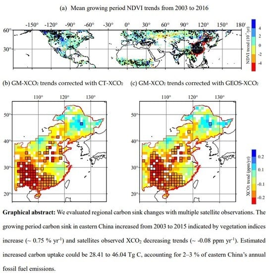
:Persistent and widespread increase of vegetation cover, identified as greening, has been observed in areas of the planet over late 20th century and early 21st century by satellite-derived vegetation indices. It is difficult to verify whether these regions are net carbon sinks or sources by studying vegetation indices alone. In this study, we investigate greening trends in Eastern China (EC) and corresponding trends in atmospheric CO2 concentrations. We used multiple vegetation indices including NDVI and EVI to characterize changes in vegetation activity over EC from 2003 to 2016. Gap-filled time series of column-averaged CO2 dry air mole fraction (XCO2) from January 2003 to May 2016, based on observations from SCIAMACHY, GOSAT, and OCO-2 satellites, were used to calculate XCO2 changes during growing season for 13 years. We derived a relationship between XCO2 and surface net CO2 fluxes from two inversion model simulations, CarbonTracker and Monitoring Atmospheric Composition and Climate (MACC), and used those relationships to estimate the biospheric CO2 flux enhancement based on satellite observed XCO2 changes. We observed significant growing period (GP) greening trends in NDVI and EVI related to cropland intensification and forest growth in the region. After removing the influence of large urban center CO2 emissions, we estimated an enhanced XCO2 drawdown during the GP of −0.070 to −0.084 ppm yr−1. Increased carbon uptake during the GP was estimated to be 28.41 to 46.04 Tg C, mainly from land management, which could offset about 2–3% of EC’s annual fossil fuel emissions. These results show the potential of using multi-satellite observed XCO2 to estimate carbon fluxes from the regional biosphere, which could be used to verify natural sinks included as national contributions of greenhouse gas emissions reduction in international climate change agreements like the UNFCC Paris Accord.
1. Introduction
Greening trends appear over much of the global land area [1], indicating changes in ecosystem function at regional scales. Atmospheric carbon dioxide (CO2) fertilization, temperature, and precipitation changes account for most of the greening of the Northern Hemisphere (NH) over the past two decades [2,3,4]. Terrestrial greening in cold climate zones is considered primarily due to warming temperature [5]. Greening may also be caused by the precipitation changes in cool-arid systems like Northern China and Mongolia [6]. In addition to changing climate, vegetation greening can also be related to forest regrowth following the abandonment of agricultural lands or plantations [7]. The drivers of greening are fairly well understood and correspond to changes in photosynthetic CO2 uptake [2,4]. However, relating these changes in vegetation indices to changes in net carbon fluxes is challenging, because they are largely insensitive to CO2 release by respiration fluxes [8].
Large-scale land management in certain areas, including agricultural expansion and intensification and afforestation and reforestation efforts, is expected to alter net carbon uptake at the local to regional scales. China’s land management policies have promoted both of these practices in recent decades [9,10,11,12,13]. Globally, agricultural production has intensified from the last century to maintain food production for population growth [14,15]. Mixed influences on carbon fluxes have been shown, for example, increased carbon uptake due to longer growing seasons [16] or intensification [17] but stronger carbon emissions from the conversion of natural systems to cultivated crops [18]. Sustainable cropland intensification is necessary for China using available arable land and water [10]. If done properly, it has the potential to reduce greenhouse gas emissions, through careful management of soil, nutrients, and water [19].
Forests are significant contributors to the global terrestrial carbon sink [20], absorbing approximately one-quarter to one-third of the anthropogenic CO2 emissions. Planted forests (afforestation and reforestation) may be used to offset anthropogenic CO2 emissions [21]. Planted forests across China increased significantly at the end of 20th century, increasing the carbon density from 15.3 to 31.1 mega-grams per hectare [22]. Forests planted by China’s Grain for Green Program, started in 1999, are estimated to have increased natural carbon sequestration, thereby mitigating CO2 emissions from fossil fuel and cement production [12,13] by about 3–5% of China’s annual carbon emissions (relative to 2010 emissions), which may continue for next 40 years as these forests continue to grow [11]. Even though the precise forest area change is difficult to estimate, the terrestrial carbon sink increase over China is generally accepted [9,23], with a net sink in the range of 0.26 Pg C per year absorbing 28–37% of the country’s cumulated fossil carbon emissions during the 1980s and 1990s [9,23,24].
In addition to vegetation indices, atmospheric CO2 concentrations using column-averaged CO2 dry air mole fraction (XCO2) provide an alternative way to investigate terrestrial biosphere carbon flux changes [25]. XCO2 represents the total amount of CO2 in a vertical column through the atmosphere, and therefore is less sensitive to changes in boundary layer height and surface winds that impact a concentration measurement near the surface without necessarily a corresponding change in local CO2 fluxes. Regional CO2 fluxes have been inferred using satellite observed XCO2 and atmospheric transport models, even though some challenges exist, like satellite observations coverage, systematic errors of the retrievals, and systematic errors of the transport models [26,27]. XCO2 seasonal cycle changes are strongly correlated with vegetation indices from satellite observations from 2009 to 2014 [28,29]. Extremely high XCO2 anomalies are usually accompanied by events such as extreme droughts or floods that reduce vegetation productivity [30,31]. Parazoo et al. [32] found a decrease in tropical XCO2 corresponding to the gross primary production (GPP) increase in the wet season and a XCO2 increase associated with strong biomass burning in dry season in Southern Amazonia. These studies show that XCO2 observations started in 2002 are just beginning to yield insight into variability and trends in surface CO2 fluxes as the records now extend to just over 15 years.
Regional CO2 fluxes have been inferred from satellite-observed XCO2 and in-situ surface observations using atmospheric transport models [26,27,33]. Incorporating XCO2 into atmospheric inversions improves upon sparse and location-biased in-situ surface observations and yields estimates that are less sensitive to atmospheric transport model uncertainty [34,35,36]. It has also been noted that including XCO2 constraints in atmospheric inversions shifts regional biospheric uptake from the tropics to the boreal latitudes [33]. Surface flux estimates from atmospheric inversions are most robust across large scales, like the Transcom regions [37] and diverge at sub-continental scales and smaller [35]. This is due largely to uncertainty in atmospheric transport models and the typically sparse surface CO2 constraints, which may attribute observed atmospheric CO2 anomalies to many different source/sink spatial distributions. In this analysis, we assume that observed localized spatial XCO2 anomalies are likely more sensitive to local surface CO2 fluxes in that specific region than flux estimates derived from atmospheric inversions. This is because there is finer spatial resolution in XCO2 observations than estimated inversion CO2 fluxes. Therefore, sub-continental-scale CO2 fluxes may be inferred from XCO2 anomalies directly.
Eastern China (EC) is one area with high densities of vegetation cover and greening trends. Even though there are some modeled carbon sequestration estimates of China’s Grain-to-Green Program [11,12,13], the magnitude of CO2 uptake has not been validated at the regional scale. This study aims to quantify recent trends in regional carbon uptake by quantifying changes in satellite-observed XCO2 during the growing period (GP). We adopt various satellite-observed vegetation parameters to characterize the seasonality and locations of increased vegetation photosynthetic activity in EC and examine XCO2 trends in those regions specifically.
2. Data and Methods
Eastern China (EC) mainland, a large carbon storage area in the mid-latitudes [24], was selected for this case study evaluation of carbon uptake trends because it shows persistent vegetation greening (Section 3.1) (outlined in red in Figure 1). Land cover consists of forest, irrigated and rain-fed cropland, and grassland in south (<34°N) and north (>=34°N) parts of EC.
Datasets used in this research are summarized in Table 1. They include four categories: (1) Vegetation parameters, including normalized difference vegetation index (NDVI), enhanced vegetation index (EVI), leaf area index (LAI), and gross primary production (GPP); (2) XCO2 time series based on observations from multiple greenhouse gas satellites, including Scanning Imaging Absorption spectrometer for Atmospheric Chartography (SCIAMACHY) onboard the Environmental Satellite (ENVISAT), Greenhouse Gases Observing Satellite (GOSAT), and Orbiting Carbon Observatory 2 (OCO-2); (3) CO2 fluxes and corresponding modeled XCO2 concentrations from two inversion models, CarbonTracker (CT) 2017 and Monitoring Atmospheric Composition and Climate (MACC-III), and one forward model GEOS-Chem v11.4; (4) supporting independent datasets, including tree canopy cover percentage (TCCP) and climate factors like land surface temperature (LST) and precipitation, are described in more detail in Section 2.4.
2.1. Trends in Regional Vegetation Indices
2.1.1. Multiple Vegetation Parameters
Satellite observed vegetation indices, included normalized difference vegetation index (NDVI) and enhanced vegetation index (EVI) from Moderate-Resolution Imaging Spectroradiometer (MODIS) (MOD13C1 v6) [38] and NDVI from Advanced Very-High-Resolution Radiometer (AVHRR) (GIMMS 3g) [39] were used for greening trend analysis. Leaf area index (LAI), indicating vegetation canopy, from MODIS (MCD15A3H v6) [40] and AVHRR (NOAA CDR v4) [41], were also used for estimating vegetation growth. In addition, GPP (MOD17A2H v6) [42] from MODIS was also used for identifying the trend of photosynthetic productivity.
MOD13C1 v6 was downloaded from National Aeronautics and Space Administration (NASA: https://search.earthdata.nasa.gov/). GIMMS 3g was from National Oceanic and Atmospheric Administration (NOAA: https://data.nodc.noaa.gov/). MCD15A3H v6, MOD17A2H v6, and NOAA CDR v4 were retrieved from Google Earth Engine [54]. NDVI/EVI from MOD13C1 v6, LAI, and GPP were resampled to temporal and spatial resolution of 16 days and 1 × 1 degree using bilinear interpolation. NDVI from GIMMS 3g was also integrated to 1 × 1 degree.
2.1.2. Growing Period Identification
Vegetation indices are widely used to characterize phenology [55,56,57]. We adopted an exponential and logistical smoothing function [57] to fit EVI time series to quantify the beginning and end of strong vegetation activity as the growing period (GP), shown in Equation (1).
where t is time in days, is the EVI value at time t, a and b are fitting parameters, and c and d were used to constrain the range of EVI values. The spatial/temporal resolution of EVI used here is in 1 × 1 degree/16-day. The start/end of GP for each grid cell can be defined as minimum/maximum value of derivation of the curvature of the function fitted to either the early season data or the late season data separately (Figure 2, the period between two red dashed lines). We excluded grid cells with poorly constrained GP from our analysis including those starting after July, ending before April, or extending for longer than 12 months as these are unrealistic results. The start, end, and length of the GP in each grid cell used for the trend analysis shown in Figure S1. The GP length retrieved in EC was 149 ± 36 days, which started from day of year 126 ± 27 and went to day of year 275 ± 16 with longer GP lengths in the south and shorter in the north (Figure S1).
2.1.3. Vegetation Indices Trend Calculation
We analyzed the trends of multiple vegetation parameters, including NDVI, EVI, and LAI, with a spatial resolution of 1 × 1 degree and time resolution of 15–16 days. After the GP was uniquely defined for each grid cell (Section 2.1.2), the mean of the vegetation indices over the fixed GP length for each year in each grid cell was calculated. Interannual trends in mean GP vegetation indices were defined using least-square linear fitting, and the Mann–Kendal test was used to determine statistical significance of the linear trends in each grid cell.
2.2. Trends in Regional XCO2 Summer Drawdown
2.2.1. Satellite-Observed XCO2
Multiple satellite-observed XCO2 products derived from SCIAMACHY, GOSAT, and OCO-2 platforms were integrated to obtain the longest and most complete record possible [58]. SCIAMACHY on-board the European ENVISAT was launched in 2002, with a temporal resolution of 36 days and spatial resolution of 60 km, available from 2003 to 2012 [59]. GOSAT was launched in 2009 by Japan, with a temporal resolution of 3 days and spatial resolution of 10 km, available from 2009 to the present [60]. NASA’s OCO-2 was launched in 2014, with a temporal resolution of 16 days and spatial resolution of 1.29 × 2.25 km at nadir, available from 2014 to present [61]. SCIAMACHY XCO2 was retrieved by the full-physics based Bremen Optimal Estimation–DOAS (BESD) algorithm (v02.01.01), referred to as BESD-XCO2 [43,44] and was downloaded from the European Space Agency (ESA, http://www.esa-ghg-cci.org/). GOSAT was retrieved by the Atmospheric CO2 Observations from Space (ACOS) project team (v7.3), referred to as ACOS-XCO2 [45]. OCO-2 was retrieved by the OCO-2 team (v7r), referred as OCO-XCO2 [46]. ACOS-XCO2 and OCO-XCO2 were downloaded from NASA (https://disc.gsfc.nasa.gov/). XCO2 from these different observations during 2003 to 2016 was integrated and mapped, described in Section 2.2.2, into global maps of XCO2 (referred as GM-XCO2) with temporal and spatial resolution of 8 days and 1 × 1 degree.
2.2.2. Merging and Gap-Filling XCO2 Data Products (Integration and Mapping)
In order to construct a long-term XCO2 dataset, BESD-XCO2 from January 2003 to May 2009, ACOS-XCO2 from June 2009 to August 2014, and OCO-XCO2 from Sep 2014 to March 2016 were used for XCO2 integration and mapping. XCO2 integration and mapping is the extension of the spatio-temporal geostatistical mapping method applied to multiple satellite observations. Corrections were made to account for differences in vertical measurement sensitivity, differences in satellite overpass times and fields of view, and observation gaps. Steps included: (1) Applying an averaging kernel correction based on vertical profiles from CarbonTracker, (2) normalizing overpass times and unifying spatio-temporal scales of multi-satellite XCO2 data, and (3) global land mapping of XCO2 based on spatio-temporal geostatistics.
In the first step, we corrected for differences in altitude sensitivity of the sensors and normalized the measurements using averaging kernels and a-priori vertical profiles of CO2 from CarbonTracker (CT-XCO2) selected as the common proxy for adjustment (Equation (2)) [43,62].
where is the adjusted XCO2 value at observation time t, corresponds to retrieved XCO2 of BESD, ACOS, or OCO-2, h and A are the pressure weighting functions and column-averaging kernels from the retrieval algorithm, respectively, I is an identity matrix, is the common priori CO2 profile from CT, and is a priori CO2 profile from satellite retrievals.
Considering the diurnal variability in XCO2 and differences in satellite overpass times, step 2 unified XCO2 from multiple satellites to a common observing local time and spatial resolution. We introduced a scale factor derived from the diurnal variation of XCO2 using CT-XCO2 to normalize the overpass time of XCO2 retrievals from these three satellites to a reference time (Equation (3)).
where is the normalized satellite-observed XCO2 at the reference time (rt: 13:00, local time); is the adjusted satellite XCO2 derived from Equation (2) at satellite overpass time t; and are the XCO2 from CT model at the reference time rt and satellite overpass time t, respectively.
Additionally, we unified the different field of views (30 × 60 km, diameter of 10.5 km and 2.25 × 1.5 km, respectively) and repeat cycles (36 days, 3 days, and 16 days, respectively) of SCIAMACHY, GOSAT, and OCO-2 before using a gap-filling method. In this study, we used a uniform spatio-temporal scale of 30 × 30 km as a space unit and 8-day as a time unit to average of BESD-XCO2, ACOS-XCO2, and OCO-XCO2 respectively. This uniform spatio-temporal scale was introduced to aggregate different XCO2 data products in order to maintain as much as possible the spatial (regional and national) and temporal (monthly and seasonally) variation of XCO2 observed by these three satellites. The integrated XCO2 dataset in 30 × 30 km and 8 days was generated from 2003 to 2016, hereafter referred to as integrated-XCO2. The data quantity and trends of integrated-XCO2 from 2003 to 2016 is shown in Figure S2.
In step 3, we applied a gap-filling interpolation method to the integrated XCO2 to produce continuous global XCO2 maps in time and space. The spatio-temporal geostatistical mapping method, GM-XCO2, applied in GOSAT observations has been previously used in global carbon research studies [28,31,63,64]. Considering the spatial connectivity used in variogram modelling, we divided global land area (within 45°S–60°N) into five continents. As different atmospheric transport exists between hemispheres, Africa was separated into North Africa and South Africa. As a result, modelling the spatio-temporal correlation structure using variograms of XCO2 in the gap-filling method was implemented for each of the six land regions: North America, South America, North Africa, South Africa, Europe, and Asia and Oceania, as shown in Figure S3. Detailed information about the spatio-temporal interpolation method can be found in Zeng et al. [63,64]. GM-XCO2 from Europe and Asia was used in the XCO2 trend analysis over EC.
GM-XCO2 data was evaluated using cross-validation (Figure S4) and by comparing to TCCON measurements (Figure S5) [28,31,64]. The predicted XCO2 (GM-XCO2) shows a significant linear relationship with the integrated-XCO2 with R2 = 0.97 (p-value < 0.01). Good agreement of integrated-XCO2 and the gap-filled GM-XCO2 is shown by the mean predicted error, mean absolute predicted error, and standard deviation of the error equal to −0.02, 0.99, and 1.38 ppm, respectively.
2.2.3. Model Simulations of XCO2 and CO2 Fluxes
Estimated surface CO2 fluxes and XCO2 concentrations from the GEOS-Chem, CarbonTracker, and MACC models were used for two purposes: (1) To create estimates of XCO2 background increase in the study area (Section 2.2.4), and (2) estimate relationships between local surface CO2 fluxes and XCO2 variability (Section 2.3). CarbonTracker (CT) 2017 is a global inversion model from NOAA providing atmospheric CO2 mixing ratio distributions and inferred surface CO2 fluxes with a time resolution of 3 h [47]. It uses the Carnegie–Ames–Stanford Approach (CASA) land surface model to estimate prior flux estimates and Transport Model 5 (TM5) to represent atmospheric circulation [65]. Optimized posterior surface flux components were solved for with a spatial resolution of 1 × 1 degrees including fossil fuel, fire, ocean, and biosphere. Each surface flux was tagged to create associated CO2 concentrations in 25 vertical atmospheric levels with spatial resolution of 2 degrees in latitude and 3 degrees in longitude. The atmospheric pressure of the different levels used was from the CT CO2 total files. Contributions to XCO2 from each component and background concentration were calculated from the vertical profiles based on the pressure-averaged method [66]. MACC-III is also an inversion model from the European Space Agency (ESA) providing global XCO2 and net CO2 fluxes with a temporal and spatial resolution of 3 h and 1.875 degrees latitude and 3.75 degrees longitude [48]. Both inversion model results have been compared to the FLUXCOM product in Asia [67], but as both are prone to different types of errors and uncertainties, there is no way to provide a robust validation of these model products.
In order to separate local biospheric CO2 flux influence in Eastern China from remote biospheric and other non-biospheric CO2 flux influences on that region, we created estimates of various CO2 flux components using transport model simulations. These simulation results were later used to remove other non-local and non-biospheric influences from observed GM-XCO2 trends using detrending methods. GEOS-Chem is a global 3-D transport model for atmospheric trace gas simulation driven by meteorological and surface flux input [49]. We adopted GEOS-Chem version 11.4 driven by MERRA-2. In the GEOS-Chem global CO2 simulation, we used the CarbonTracker fossil fuel, ocean exchange, and biosphere posterior CO2 fluxes to replace the standard GEOS-Chem surface CO2 flux input. The biomass fire emissions were taken from the Global Fire Emission Database version 4.1s (GFEDv4.1s) [68]. We used annually neutral net terrestrial exchange fluxes and turned off ship and aviation emissions and the 3-D Chemical Oxidized Source. Fossil fuel CO2 emissions used in these tracer models were from the Open-source Data Inventory for Anthropogenic CO2 (ODIAC), which is a global anthropogenic CO2 emission dataset based on estimates made by the Carbon Dioxide Information and Analysis Center (CDIAC) and satellite-observed nightlights and the power plant profile dataset for spatial and temporal distributions [51]. It is monthly data with a spatial resolution of 1 × 1 degree.
The global background and a nested GEOS-Chem simulated XCO2 for Eastern Asia (referred as Back-GEOS-XCO2 and Nested-GEOS-XCO2, respectively) were used for local XCO2 background corrections without introducing modeled local biosphere flux variability. In the nested Eastern Asia CO2 simulation, we used the GFED 4.1s land net ecosystem exchange, CarbonTracker biosphere prior CO2 fluxes with annually neutral net CO2 fluxes instead of the CarbonTracker biosphere posterior CO2 fluxes, which are time-varying from year-to-year. The boundary conditions used for the GEOS-Chem nested grid model in eastern Asia at 0.5° (latitude) × 0.625° (longitude) simulation were provided by the global background model at 2° (latitude) × 2.5° (longitude) horizontal resolution. We made a restart file with 3-D CO2 concentrations from CarbonTracker at 0:00, on Jan 1 of 2003. The resolution from 25 vertical layers and 2° × 3° in CT to 47 vertical layers and 2° × 2.5° in GEOS-Chem, was resampled using the nearest neighbor method. Model CO2 profiles (averages for 12:00–14:00 local time) and the pressure-weighting function described in [66] were used to convert modelled CO2 in discrete layers to XCO2. Temporal mean values of GEOS-Chem background and GEOS-Chem nested simulated XCO2 from 2003 to 2016 over Eastern Asia are shown in Figure S6.
In addition, changes in the sum of XCO2 components (XCO2 changes resulting from fossil, fire, biosphere, and ocean CO2 fluxes) from CT and the MACC-III inversion models were used to estimate relationships between local surface CO2 fluxes and XCO2 variability described in Section 2.3.
2.2.4. XCO2 Detrending Methods
To quantify local biosphere-driven changes in XCO2 over time, we need to remove the background XCO2 increase due to sustained fossil fuel emissions and influence from ocean exchange and fire, as well as remote biospheric influence from the study region [69,70]. The precise influence of all non-local non-biospheric processes cannot be directly measured, so we tested four different approaches for defining the background trend to isolate the local biospheric influence in the GM-XCO2 record. For a first approximation, we adopted the global mean yearly increase from NOAA (https://www.esrl.noaa.gov/gmd/ccgg/trends/gr.html) to build a global background XCO2 increase and applied that uniformly to all grid cells in the study region. The three other detrending methods were based on curve-fitting long-term trends, calculated and applied on a grid cell-by-cell basis. For one, we used the long-term trend XCO2 increase from the gridded GM-XCO2 observations themselves. In another, we used the fitted XCO2 gridded results from CT-XCO2. Finally, we fitted the global background and nested GEOS-Chem simulated XCO2 to clarify the remote influences from the local influences.
The curve-fitting equation applied to each of the three XCO2 records used a combination of a step-wise linear function and annual periodic function as shown in Equation (4).
Here, is XCO2 in time t, and are treated as the background and cumulated increase of XCO2 in each year, and is used for characterizing the XCO2 seasonal cycle. An example of GM-XCO2 and CT-XCO2 fitting of 13 years in one grid cell (Lat: 38.5°N; Lon: 115.5°E) over EC is shown in Figure 3. Because fitting trends for individual years leads to discontinuities due to the start and end values, we used the mean value of three fitting results using 3 different time windows, starting from 1 December of previous year, 1 January, or 1 February of that year. Example curve fits are shown in Figure 3, but different patterns may be observed at other grid cells. The background XCO2 increase (y) in year i and day j are extracted from the non-seasonal portion of Equation (4) and can be interpolated to daily values using Equation (5).
where and are the fitted XCO2 background () and increase ratio () in year i (from Equation (4) fit), n is the total units in one year (‘365′ used for daily data and ‘46′ used for data with time resolution of 8 days), and j is the current time step (day or number of 8-day interval). The yearly fitting performed well in global/site CO2 yearly increase with differences of −0.04 ± 0.27 ppm for NOAA global mean, −0.03 ± 0.13 ppm for global mean of CT-XCO2, and −0.06 ± 0.19 ppm for Mauna Loa shown in Figure S7 and Table S1.
2.2.5. Quantifying XCO2 Trends
Global detrended GM-XCO2 maps derived from integrated and gap-filled satellite observations with temporal and spatial resolution of 8 days and 1 × 1 degree were examined for growing period (GP) drawdown trends from 2003 to 2015. The GP was defined for each grid cell using the EVI analysis presented in Section 2.1.2 and the mean GP value of the detrended GM-XCO2 was calculated for each grid cell and for each year. Least-squares linear fitting and the Mann–Kendal test were used to calculate XCO2 trends and significance for each grid cell.
2.3. Estimating Surface CO2 Fluxes from XCO2 Variability Based on Correlations in Inversion Models
XCO2 variability is closely related to surface CO2 fluxes, however quantifying that relationship is challenging due to uncertainties in atmospheric transport and remote versus local CO2 contributions. To estimate the magnitude of the surface flux responsible for observed trends in XCO2, we derived a relationship between surface CO2 fluxes and atmospheric XCO2 from model simulations including CarbonTracker and MACC-III across different time and spatial scales: Daily and 16 days and global and grid cells in EC regions (shown in Figure 1). The total area of selected grid cells in EC shown in Figure S8 is 4.47 × 10¹² m2. As the regions become smaller, we expected more noise in the correlations due to transport of CO2 in/out of the region. We also examined the relationship over different time intervals. Daily XCO2 changes were calculated from the difference between two consecutive days and compared to the daily mean CO2 flux. The daily XCO2 and CO2 flux changes from 1 January 2003 to 31 December 2016 in each grid cell were calculated using CT and MACC. XCO2 changes of several days were defined as the sum of daily changes and CO2 flux changes were defined as total CO2 fluxes of these days. Correlation analysis and least-squares fitting were calculated for the flux-XCO2 relationships (defined as transform ratios) at these different time and space scales. For this analysis of EC, we chose the 16-day correlation over EC to estimate CO2 flux anomalies from XCO2 changes.
2.4. Supporting Independent Datatsets
2.4.1. Vegetation Coverage Changes
We compared trends in atmospheric XCO2 to independent evidence of vegetation changes in EC. We adopted tree canopy cover percentage (TCCP) from global vegetation continuous fields (VCF) products by Song et al. [50], which were retrieved from the NASA website (https://search.earthdata.nasa.gov/). This vegetation continuous field was developed using daily satellite AVHRR observations. Tree canopy cover percentage with a spatial resolution of 0.05 × 0.05 degree was resampled to 1 × 1 degree, same as that of vegetation parameters and GM-XCO2 used in this analysis.
2.4.2. XCO2 from TCCON Measurements
TCCON is a global network of ground-based Fourier transform spectrometers for atmospheric XCO2 and other trace gases measurements [71]. We compared GM-XCO2 retrievals to these ground-based measurements to identify potential measurement biases. XCO2 retrievals from TCCON has a high accuracy with approximately 0.25%, which can be used for validation of satellites observed XCO2 [72]. In this study, we selected atmospheric CO2 measurement from TCCON sites with data between 2003.01 to 2016.03 for GM-XCO2 validation. These sites include Bialystok, Bremen, Karlsruhe, Orleans, Garmisch, Park Falls, Lamont, Tsukuba, Edwards, JPL/Caltech, Saga, Manus, Darwin, Wollongong, and Lauder. Locations of former 11 sites in northern hemisphere are shown in Figure 1, and other the 4 sites (Manus, Darwin, Wollongong, and Lauder) in the southern hemisphere are inside of Brazil, north and south of Australia, and New Zealand, respectively. TCCON measurements from Jan 2003 to Mar 2016, observing local time during 11:00 to 15:00 were used for XCO2 comparison. As a result, there were 3603 pairs of GM-XCO2 and TCCON XCO2, from 15 TCCON sites, used for comparison (GM-XCO2 minus TCCON XCO2). R2, mean bias, mean absolute bias, and standard deviation between them were 0.96, 0.20, 0.90, and 1.16, respectively.
2.4.3. Climate Factors
Land surface temperature (LST) and precipitation were used for evaluating the effects from climate change in XCO2 change. LST from MODIS (MOD11C2 v6) [52] was downloaded from NASA (https://search.earthdata.nasa.gov/). Precipitation from the Tropical Rainfall Measuring Mission (TRMM) v3B42 [53] was obtained from Google Earth Engine. LST and precipitation were resampled to temporal and spatial resolution of 16 days and 1 × 1 degree for correlation analysis with corrected XCO2.
3. Results
3.1. Trends in Regional Vegetation Parameters
Here, we show mean growing period (GP) vegetation trends for MODIS NDVI and AVHRR NDVI from 2003 to 2016 and AVHRR LAI and tree canopy cover trends from 2003 to 2016 (Figure 4). These vegetation indices are unitless because NDVI and EVI range 0–1 and LAI is in m2 of leaf area per m2 land surface area. MODIS EVI, LAI, and GPP trends during the GP from 2003 to 2016 are shown in Figure S9. Significant greening trends were observed in EC (Eastern China with red edge) with similar patterns in MODIS NDVI, AVHRR NDVI, and MODIS EVI (Figure 4a,b and Figure S9a). The trends in mean GP values of MODIS NDVI, AVHRR NDVI, and MODIS EVI over EC from 2003 to 2016 were 0.38 ± 0.27 × 10⁻² yr−1, 0.38 ± 0.30 × 10⁻² yr−1, and 0.32 ± 0.21 × 10⁻² yr−1, which accounted for 0.70 ± 0.61% yr−1 and 0.71 ± 0.75% yr−1 of NDVI (MODIS and AVHRR, respectively) and 0.86 ± 0.60% yr−1 of EVI relative to the mean values over this 14-year period. The standard deviation reported here is the variability in all grid cells trends across the EC domain and not an indicator of within-grid cell trend uncertainty. AVHRR LAI also showed significant increasing trends in EC with 0.013 ± 0.010 m2 m−2 yr−1 (Figure 4c). In addition, increasing trends (0.009 ± 0.010 m2 m−2 yr−1 and 0.11 ± 0.19 g C m−2 yr−2) of LAI and GPP from MODIS were also significant in most area of Eastern China (Figure S9). Total increases of NDVI and GPP over Eastern China from 2003 to 2015 could be around 8.40% to 8.52% and 9.24 g C m−2, respectively.
Tree canopy annual trends from 2003 to 2016 showed a strong net increasing trend (0.65 ± 0.34% yr−1) in the southern part of EC (Figure 4d, latitude < 34°N). Large total tree canopy increase from 2003 to 2015 (7.80%), potentially resulting in enhanced photosynthesis rates, may have increased the net carbon sink in this region.
3.2. Trends in Regional XCO2 Summer Drawdown
Here we identify the trends in GM-XCO2 that best reflect local biospheric processes in EC and present different methods for removing the influence from fossil fuel and fire emissions and ocean exchange from the observations, and in some cases, remote biospheric influence.
3.2.1. Satellite Observed XCO2 Trends after Removing Global Mean Growth
As a first attempt, we removed the NOAA global mean XCO2 growth rate from the GM-XCO2 in order to calculate summer drawdown trends using the mean value of detrended GM-XCO2 during the GP of each year as shown in Figure 5a. This removed remote influence, the long-term atmospheric growth rate, at each grid cell. Red grid cells with black outlines, indicating significant decreasing trends, were observed in some parts of south China (−0.07 ± 0.05 ppm yr−1 for decreasing grid cells). Blue grid cells with black outlines, indicating significant increasing trends, 0.05 ± 0.05 ppm yr−1, were observed in some urban regions like Beijing and Shanghai.
Regions around cites like Beijing and Shanghai showed increasing XCO2 at more extreme rates than the global mean. Blue grid cells indicate CO2 emission increases (0.045 ± 0.055 kg C m−2 yr−2) near urban centers of Eastern Asia in Figure 5a. This is because fossil emissions have increased faster in Beijing and Shanghai than most other regions. Gridded trends in anthropogenic emissions from January 2003 to December 2016 from ODIAC are shown in Figure 5b. Therefore, it is necessary to remove the influence of the local urban CO2 emission domes in order to isolate trends in local biospheric influence on XCO2.
3.2.2. Satellite-Observed XCO2 Trends after Removing Influence of the Urban CO2 Dome
In order to remove the influence of increasing anthropogenic emissions from urban centers in our study area, we tested four different spatially variable methods of detrending GM-XCO2 observations: GM-XCO2 fitting (Figure 6a), CT-XCO2 fitting (Figure 6b), and GEOS-Chem simulated XCO2 fitting at two different spatial scales: a coarse 2 × 2.5 degree lat/lon simulation and a high-resolution nested simulation for Eastern Asia (Figure 6c–d). All methods showed GM-XCO2 residuals decreasing in many EC grid cells from 2003 to 2015 indicating greater CO2 uptake during the GP. For the entire EC domain, detrending the XCO2 time series of each grid by the long-term trend of each grid cell (GM-XCO2 detrending using the full record including growing season and dormant season) resulted in a small trend in the corrected GM-XCO2 during the GP, −0.058 ± 0.029 ppm yr−1. The standard deviation reported here is the variability in individual grid cell trends across the EC domain and not an indicator of within grid cell trend uncertainty. This is possible because the annual means and the GP drawdown only can have different trends as seasonal cycles change over time. Detrending using model simulations of XCO2 from remote and local non-biospheric CO2 fluxes resulted in larger GP CO2 uptake trends: −0.084 ± 0.090, −0.081 ± 0.088, and −0.070 ± 0.093 ppm yr−1 (mean ± 1 standard deviation in space), for CT-XCO2 and GEOS-Chem coarse and fine resolution, respectively. Of all the grid cells, larger GP CO2 uptake trends were observed in 80%, 79%, and 77% of the grid cells depending on the correction method applied, CT-XCO2 fitting, and GEOS-Chem fittings at coarse and fine resolution, respectively. Grid cells with statistically significant (p < 0.05) increasing GP CO2 uptake trends occupied 40%, 41%, and 39% of EC, respectively. The trends for just the grid cells that showed increased CO2 uptake were −0.116 ± 0.067, −0.113 ± 0.069, and −0.108 ± 0.068 ppm yr−1, respectively (mean ± 1 standard deviation in space).
The similar pattern of trends of these last three correction methods showed that there was robust evidence of increased GP CO2 uptake in EC due to biological activity. We consider the corrected GP trend using the GM-XCO2 annual increase of −0.058 ppm yr−1 to be the lower estimate of biospheric influence on EC CO2 uptake because the local biospheric influence is in the GM-XCO2 signal itself and a portion of it is removed by the fitting. CT-XCO2 should depict the general pattern of atmospheric CO2 concentration over city areas, as the posterior CO2 concentration and flux from CT includes fossil fuel emissions and was the optimum estimate of the inversion model.
The spatial patterns of corrected GM-XCO2 decreases were similar to the increases in vegetation indices, south of the urban centers, shown in Figure 4 and Figure S9a. These results indicate vegetation increases have been accompanied by stronger photosynthesis rates during the GP from 2003 to 2016 and imply increased carbon uptake in EC during the growing season.
3.3. Trends in Flux Estimates
The corrected GM-XCO2 trends of −0.070 to −0.084 ppm yr−1 in EC suggest an increased biospheric uptake. In order to estimate the magnitude of the surface CO2 fluxes that would produce that XCO2 anomaly, we used the CT and MACC models to relate CO2 fluxes to atmospheric CO2 concentration anomalies. We explored correlation between model simulated XCO2 changes daily or over 16 days and net CO2 flux changes in the global or EC region shown in Figure 7. Significant and strong positive correlations were found in the global daily mean data both from CT (Figure 7a, R2 = 0.84, p < 0.01) and MACC (Figure 7d, R2 = 0.49, p < 0.01) with slopes approaching 0.26 ppm/(g C/m2/day) from CT and 0.21 ppm/(g C/m2/day) from MACC, where the former was a little larger. The correlation and slopes over EC were much lower than that in the global mean, but still significant (Figure 7b–d). This is because at the global scale, CO2 is conserved during atmospheric transport within the global domain, whereas at the regional domain, transport can be a source or sink of CO2. The correlation decreased as the domain considered got smaller from global to EC. The correlation from daily to 16 days (the time resolution of satellite observed XCO2 and vegetation parameters) became stronger both for CT (Figure 7c) (R2 = 0.26, p < 0.01) and MACC (Figure 7f) (R2 = 0.23, p < 0.01). The flux-XCO2 transform ratios of 16-day were similar for CT (0.0523 ppm/(g C/m2/16days)) and MACC (0.0465 ppm/(g C/m2/16days)). The correlation became stronger as the time interval increased (from daily to 16-day means), because the influence of persistent CO2 fluxes built up within the domain.
We estimated the CO2 flux change from the corrected GM-XCO2 trends and the model correlation between XCO2 16-day changes and CO2 flux change shown in Table 2. The total XCO2 change were estimated as −1.008 ± 1.080, −0.972 ± 1.056, and −0.840 ± 1.116 ppm (standard deviation represents spatial variability) from 2003 to 2015 for different correction methods (CT-XCO2 fitting, background GEOS-XCO2 fitting, and nested GEOS-XCO2 fitting). The inferred carbon uptake increase mean value over the region and its spatial variability were 9.57 ± 10.94, 8.88 ± 10.48, and 6.36 ± 11.63 g C/m2 using the CT ppm-to-flux transform ratio and 10.30 ±11.85, 9.52 ± 11.33, and 6.69 ± 12.62 g C/m2 using the MACC transform ratio. That is basically consistent with GPP increase of 9.24 g C m−2 shown in Section 3.1. The total carbon uptake amount from 2003 to 2015 ranged from 28.41 to 46.04 Tg C with an EC region area of 4.47 × 10¹² m2 shown in Figure S8.
To put this carbon uptake into perspective, we compared it to the carbon exchange inferred from CT during the GP (from day 126 to 275) and the whole year in this region. The averaged biospheric CO2 flux during the GP during 2003 to 2016 over EC was −99.8 ± 30.6 g C m−2 yr−1 (uncertainty is 1 standard deviation of inter-annual variability). Annual fossil fuel CO2 emission for the same period was 328.48 ± 91.38 g C m−2 yr−1 (uncertainty is 1 standard deviation of inter-annual variability). The satellite-observed total carbon uptake increases from 2003 to 2015 accounted for 6.4% to 10.3% of the mean biosphere flux during the GP, approaching the percentage increase in the vegetation indices of 8.4% to 10.3% from 2003 to 2015. This uptake could offset 1.9% to 3.1% of annual fossil carbon emissions over that region.
3.4. Possible Contribution from Climate Variability, Independent of Land Management
To check the relationship between XCO2 and climate change, we present the Pearson correlation coefficients between corrected XCO2 and MODIS land surface temperature (LST) and TRMM precipitation during the GP from 2003 to 2016 shown in Figure 8. In EC, there was no significant correlation between corrected XCO2 and temperature. This is because vegetation growth is not temperature-limited due to already warm temperatures (Figure S10a) and there were no significant grid-cell trends in LST (Figure S10c). The correlation between corrected XCO2 and precipitation was also not significant. The precipitation in the southern part of EC increased and in the northern part decreased (Figure S10d). A decrease in rainfall in that region was unlikely to result in increased CO2 uptake. Vegetation growth was limited by water in the northern region (Figure S10b), which is why water diversion projects have been constructed to transfer water to the north, therefore disconnecting CO2 uptake from precipitation. Overall, there is no strong support for the observed EC greening trends to be caused by changes in regional temperature and rainfall. It is more likely that greening patterns are driven by increased irrigation in Northeastern China [22,73] and land use change in Southeastern China [74].
4. Discussion
Vegetation greening trends (Figure 4) and XCO2 decreasing trends (Figure 6) during the GP show similar patterns of enhanced greening and CO2 uptake in Eastern China (EC). This indicates that enhancements in vegetation activity have had a measurable influence on regional atmospheric XCO2 concentrations due to enhanced CO2 uptake during the GP. Here, we discuss the likely drivers of the vegetation changes we observed, our estimates of the flux changes associated with the XCO2 trend, and consider the uncertainty in our analysis.
4.1. Different Drivers of Greening in North and South Parts of Eastern China
Greening trends are observed throughout EC (Figure 4), however the main drivers of these trends are likely different in the north and the south. In the northern part, cropland production has increased significantly from 1987 to 2010 [10] in order to feed the large increase in Chinese population (from 1.08 to 1.34 billion). Increases in agricultural productivity come from increased cropland area [10,74,75] and increased irrigation from water diversion projects moving water from the south to the North China Plain [22,73]. In addition, increased fertilization by nitrogen and phosphorus application [76] and lengthening of the growing period due to warmer temperatures with climate change [77] could provide more nutrients and a longer period of optimal growth conditions.
In the southern part, tree canopy coverage has increased by 9.27 ± 4.93% in 2016 from 30.51 ± 13.90% in 2003 [50]. Over the last century, widespread deforestation and forest degradation occurred due to conversion to cropland, infrastructure development, mining, fire, and urbanization. During the 21st century, afforestation and reforestation increased significantly in the south part of EC [4], due to governmental policy. Climate conditions over southern EC are suitable for forest growth and expansion to increase carbon uptake with protection provided by land management policies [9].
4.2. Uncertainty of GM-XCO2 Trends
The GM-XCO2 product involves merging and gap-filling multiple satellite records (Section 2.2.2), therefore, we need to consider the uncertainty associated with this product. Spurious trends could be caused by the gap-filling method, so we checked the amount of available satellite-observed XCO2 in each grid cell over EC (Figure S11). A greater proportion of observations are distributed in the northern part of China for SCIAMACHY BESD XCO2 (2003.01–2009.05), GOSAT ACOS XCO2 (2009.06–2014.08), and OCO-2 XCO2 (2014.09–2016.03) because of the cloud contamination discussed earlier. Here, we show the temporal change of integrated XCO2 (the merging of data from the three sensors) and GM-XCO2 (gap-filled) using available data in EC as shown in Figure 9. GM-XCO2 agreed well with integrated XCO2 with a mean difference of 0.25 ± 1.33 ppm. Some differences exist during summer for distinct XCO2 spatial variations shown with mean ± 1 STD GM-XCO2 (red dashed lines). We found no significant trend in the GP residuals between integrated XCO2 and the gap-filled GM-XCO2 using the Mann–Kendal trend test. Therefore, we conclude that the XCO2 decreasing trends are not caused by the gap-filling method.
In addition, we checked the GM-XCO2 product against TCCON measurements as shown in Figure S5. The mean absolute difference (bias) between GM-XCO2 and TCCON observations with 3608 co-located data pairs was 0.90 ± 1.16 ppm. Individual grid-cell GM-XCO2 bias followed a Gaussian distribution, therefore the XCO2 uncertainty over EC was estimated as the averaged bias divided by the square root of the number of grid cells in EC. As a result, the uncertainty was less than 0.045 ppm, which is significantly less than the XCO2 total change (0.840–1.008 ppm from 2003 to 2016). XCO2 differences between GM-XCO2 and TCCON measurements from 2003 to 2016 are shown in Figure 10. The differences fluctuate around zero and present no trends from 2003 to 2016 for data pairs in the northern hemisphere. This comparison with the TCCON observations showed that there was no evidence of sensor offsets or drift that would create artificial GM-XCO2 trends over time.
4.3. Uncertainties in Constraining the Urban Dome and Remote Influence on XCO2 Trends
The XCO2 trends observed over EC result from a combination of remote and local influences. Accurately quantifying the influence of regional biospheric CO2 fluxes in EC depends on how well we remove the influence from non-local biospheric CO2 fluxes including remote and local anthropogenic fossil and fire emissions and ocean gas exchange as well as remote biospheric influence. In this study, we tested four methods for removing the cumulated XCO2 increase to better study the local biospheric component of XCO2 changes. The first method using the NOAA-reported global mean CO2 is not able to remove the influence from the local urban CO2 dome, which increases over time and therefore underestimated the trend in XCO2 due to local biospheric influence. In addition, the time series fitting of GM-XCO2 removed the local annual biospheric contribution to the XCO2 trend and underestimated the signal of interest, although there was still a component of GS trends in XCO2 that served as a lower bound of local biospheric influence. The trends calculated from detrending using simulated XCO2 using CT and GEOS-Chem transport (with and without nested grid cells) of CT surface CO2 fluxes were likely the best representation of local biospheric influence on XCO2 because they are designed to remove trends caused by the remote biospheric CO2 fluxes over time, but retain trends in local biospheric CO2 fluxes, plus remove all the non-biospheric influence. Similarities between Figure 6c,d showed that characterizing the fine spatial scale resolution of the urban XCO2 dome was not critical to defining GP trends. Therefore, XCO2 decreasing trends of −0.084 ± 0.090, −0.081 ± 0.088, and −0.070 ± 0.093 ppm yr−1 were our best estimates of XCO2 change caused by EC region local biospheric CO2 fluxes with uncertainty listed is the grid-scale spatial variability in trends (Table 2). These trends result in a total XCO2 change from 2003 to 2015 of −0.84 to −1.01 ppm.
This analysis is subject to two sources of bias. First, uncertainty in remote CO2 fluxes could result in artificial trends in local biospheric CO2 fluxes in the study region, however it is very unlikely that such an artificial signal from remote CO2 flux uncertainty would correspond to the exact region that shows vegetation greening. Second, an overestimate in local fossil fuel CO2 emissions from EC in the EDGAR database would result in an overestimate of local biospheric uptake. Saeki and Patra [78] suggested that fossil fuel CO2 emissions in EC may in fact be overestimated based on scaling with methane emissions. There is no independent way to verify local fossil emissions in EC at the moment. However, the correction method based on detrending using annual global mean CO2 concentrations from NOAA supports a local biospheric sink in the southern portion of EC in addition to showing urban emissions increasing faster than the global mean in the northern part (Figure 4a). This correction method cannot create regional artificial biospheric uptake due to local CO2 emissions uncertainty. However, the magnitude of the inferred sink is sensitive to local CO2 emissions uncertainty. This demonstrates the importance of independent constraints of fossil and biospheric CO2 fluxes in order to understand CO2 flux trends near urban centers.
4.4. Inferred Surface Flux Changes over This Period
It is predicted that China’s investments into environmental improvement has likely increased the forest carbon sink in EC [9,23,24]. However, the carbon sink over the East Asian monsoon region is difficult to measure and there is speculation that it has been underestimated [79]. We find the estimated cumulated carbon uptake increases from 2003 to 2015 was in range from 6.36 to 10.30 g C m−2 over EC. To understand the significance of these changes, we compare with mean posterior flux estimates from CT (Table 3). The carbon sink increase is equivalent to 9.0% to 14.6% of the annual biospheric flux over EC and equivalent to offsetting about 1.9–3.1% of EC’s annual fossil fuel CO2 emissions. By comparison, the increased carbon uptake during the GP was slightly underestimated in the interannually varying CT posterior CO2 fluxes, which is about 6.4% to 10.3% of regional CT posterior annual biopsheric flux.
In this estimation, we calculated the biospheric CO2 flux trend during the GP only, not including the dormant season. It is possible that carbon release during the dormant season could cancel some of the carbon uptake gains made in the GP. We tested XCO2 trends in the dormant season, after CT-XCO2 correction (Figure S12), but find no significant trends in EC. It is possible that this carbon sink could saturate in the future as the forests mature and agricultural intensification peaks [80]. These could be evaluated with continuous observations.
The method used here to infer flux changes is different from atmospheric inversion approaches [26,27] and more recent Lagrangian methods [81,82] to link surface CO2 fluxes to atmospheric CO2 observations. Our approach may likely underestimate the surface CO2 sink strength as some of the negative CO2 anomaly is transported out of the study domain. However, it is unlikely that an anomaly caused by a CO2 sink outside of the domain is transported inside because of the distribution of vegetation in this region. This analysis should be viewed as an independent method with a different sensitivity to atmospheric transport uncertainty.
5. Conclusions
Significant greening trends in Eastern China were observed by various parameters including NDVI trends of 0.70 ± 0.61% yr−1 (MODIS) and 0.71 ± 0.75% yr−1 (AVHRR) and an EVI trend of 0.86 ± 0.60% yr−1 (MODIS). Greening trends over the northern and southern parts of EC are consistent with increased cropland area and production increase in north, and forest canopy increase in south. These have previously been attributed to the national policies of sustainable development, including intensification of agriculture and afforestation and reforestation as part of China’s Grain-to-Green program [2]. Here, we show that these greening patterns are consistent with increased growing season CO2 uptake in this region.
Satellite-observed XCO2 trends showed a corresponding increase in the carbon sink in the region of greening in EC. Significant XCO2 decreases attributable to local biospheric influence during the growing period were shown using different correction methods to remove non-local, non-biospheric influence. Averaged XCO2 trends across EC varied from −0.070 to −0.084 ppm yr−1. Estimated local CO2 uptake increases were 6.36 to 10.30 g C m−2 over EC during the growing period, which is consistent with a MODIS observed GPP increase of 9.24 g C m−2. These fluxes accounted for 6.4 to 10.3% of the mean biosphere flux during the GP, which is similar to percent increases in vegetation indices, 8.40 to 10.32% from 2003 to 2015. The total carbon uptake increase ranged from 28.41 to 46.04 Tg C. That could offset about 2–3% of EC’s annual fossil fuel emissions. Integrated data from multiple greenhouse satellite (SCIAMACHY, GOSAT, OCO-2 or the recently launched Tansat) observations could provide a valuable method for estimating regional CO2 flux change.
Supplementary Materials
The following are available online at https://0-www-mdpi-com.brum.beds.ac.uk/2072-4292/12/4/718/s1.
Author Contributions
Conceptualization, L.R.W. and Z.H.; methodology, L.R.W. and Z.H.; formal analysis, L.R.W., Z.H. and L.L.; software, L.L., Z.-C.Z., and M.S.; writing—original draft preparation, Z.H. and L.R.W.; writing—review and editing, L.R.W., Z.H. and L.L. All authors have read and agreed to the published version of the manuscript.
Funding
This research was funded by the National Key Research and Development Program of China (2016YFA0600303), the Strategic Priority Research Program of the Chinese Academy of Sciences (XDA19080303) and the Key Research Program of Chinese Academy of Sciences (ZDRW-ZS-2019-3). Z.H. was supported by a University of Chinese Academy of Sciences (UCAS) Joint Ph.D. Program scholarship.
Acknowledgments
We thank Prabir Patra for productive conversations regarding this analysis. We also thank ESA for sharing the SCIAMACHY BESD XCO2 level 2 data, the ACOS/OCO-2 project at JPL for sharing ACOS-GOSAT v7.3 and OCO-2 v7r data, NOAA ESRL for proving CarbonTracker CT2017 results, and ECMWF for providing MACC-III results. We thank NASA, NOAA, and Google Earth Engine for providing vegetation indices.
Conflicts of Interest
The authors declare no conflict of interest.
References
- Zhu, Z.; Piao, S.; Myneni, R.B.; Huang, M.; Zeng, Z.; Canadell, J.G.; Ciais, P.; Sitch, S.; Friedlingstein, P.; Arneth, A.; et al. Greening of the Earth and its drivers. Nat. Clim. Chang. 2016, 6, 791–795. [Google Scholar] [CrossRef]
- Chen, C.; Park, T.; Wang, X.; Piao, S.; Xu, B.; Chaturvedi, R.K.; Fuchs, R.; Brovkin, V.; Ciais, P.; Fensholt, R.; et al. China and India lead in greening of the world through land-use management. Nat. Sustain. 2019, 2, 122–129. [Google Scholar] [CrossRef] [PubMed]
- Piao, S.; Friedlingstein, P.; Ciais, P.; Zhou, L.; Chen, A. Effect of climate and CO2 changes on the greening of the Northern Hemisphere over the past two decades. Geophys. Res. Lett. 2006, 33. [Google Scholar] [CrossRef] [Green Version]
- Piao, S.; Yin, G.; Tan, J.; Cheng, L.; Huang, M.; Li, Y.; Liu, R.; Mao, J.; Myneni, R.B.; Peng, S.; et al. Detection and attribution of vegetation greening trend in China over the last 30 years. Glob. Chang. Biol. 2015, 21, 1601–1609. [Google Scholar] [CrossRef]
- Nemani, R.R.; Keeling, C.D.; Hashimoto, H.; Jolly, W.M.; Piper, S.C.; Tucker, C.J.; Myneni, R.B.; Running, S.W. Climate-Driven Increases in Global Terrestrial Net Primary Production from 1982 to 1999. Science 2003, 300, 1560–1563. [Google Scholar] [CrossRef] [Green Version]
- Poulter, B.; Pederson, N.; Liu, H.; Zhu, Z.; D’Arrigo, R.; Ciais, P.; Davi, N.; Frank, D.; Leland, C.; Myneni, R.; et al. Recent trends in Inner Asian forest dynamics to temperature and precipitation indicate high sensitivity to climate change. Agric. For. Meteorol. 2013, 178, 31–45. [Google Scholar] [CrossRef] [Green Version]
- Xiao, J.; Moody, A. Geographical distribution of global greening trends and their climatic correlates: 1982–1998. Int. J. Remote Sens. 2008, 26, 2371–2390. [Google Scholar] [CrossRef]
- Piao, S.; Wang, X.; Park, T.; Chen, C.; Lian, X.; He, Y.; Bjerke, J.W.; Chen, A.; Ciais, P.; Tømmervik, H.; et al. Characteristics, drivers and feedbacks of global greening. Nat. Rev. Earth Environ. 2019, 1, 14–27. [Google Scholar] [CrossRef]
- Ahrends, A.; Hollingsworth, P.M.; Beckschäfer, P.; Chen, H.; Zomer, R.J.; Zhang, L.; Wang, M.; Xu, J. China’s fight to halt tree cover loss. Proc. R. Soc. B Biol. Sci. 2017, 284. [Google Scholar] [CrossRef]
- Zuo, L.; Zhang, Z.; Carlson, K.M.; MacDonald, G.K.; Brauman, K.A.; Liu, Y.; Zhang, W.; Zhang, H.; Wu, W.; Zhao, X.; et al. Progress towards sustainable intensification in China challenged by land-use change. Nat. Sustain. 2018, 1, 304–313. [Google Scholar] [CrossRef]
- Deng, L.; Liu, S.; Kim, D.G.; Peng, C.; Sweeney, S.; Shangguan, Z. Past and future carbon sequestration benefits of China’s grain for green program. Glob. Environ. Chang. 2017, 47, 13–20. [Google Scholar] [CrossRef]
- Liu, D.; Chen, Y.; Cai, W.; Dong, W.; Xiao, J.; Chen, J.; Zhang, H.; Xia, J.; Yuan, W. The contribution of China’s Grain to Green Program to carbon sequestration. Landsc. Ecol. 2014, 29, 1675–1688. [Google Scholar] [CrossRef]
- Persson, M.; Moberg, J.; Ostwald, M.; Xu, J. The Chinese Grain for Green Programme: Assessing the carbon sequestered via land reform. J. Environ. Manag. 2013, 126, 142–146. [Google Scholar] [CrossRef] [PubMed]
- Foley, J.A.; Ramankutty, N.; Brauman, K.A.; Cassidy, E.S.; Gerber, J.S.; Johnston, M.; Mueller, N.D.; O’Connell, C.; Ray, D.K.; West, P.C.; et al. Solutions for a cultivated planet. Nature 2011, 478, 337–342. [Google Scholar] [CrossRef] [Green Version]
- Matson, P.A.; Parton, W.J.; Power, A.G.; Swift, M.J. Agricultural Intensification and Ecosystem Properties. Science 1997, 277, 504–509. [Google Scholar] [CrossRef] [Green Version]
- Reyes-Fox, M.; Steltzer, H.; Trlica, M.J.; McMaster, G.S.; Andales, A.A.; LeCain, D.R.; Morgan, J.A. Elevated CO2 further lengthens growing season under warming conditions. Nature 2014, 510, 259–262. [Google Scholar] [CrossRef]
- Gray, J.M.; Frolking, S.; Kort, E.A.; Ray, D.K.; Kucharik, C.J.; Ramankutty, N.; Friedl, M.A. Direct human influence on atmospheric CO2 seasonality from increased cropland productivity. Nature 2014, 515, 398–401. [Google Scholar] [CrossRef]
- Baumann, M.; Gasparri, I.; Piquer-Rodriguez, M.; Gavier Pizarro, G.; Griffiths, P.; Hostert, P.; Kuemmerle, T. Carbon emissions from agricultural expansion and intensification in the Chaco. Glob. Chang. Biol. 2017, 23, 1902–1916. [Google Scholar] [CrossRef]
- Burney, J.A.; Davis, S.J.; Lobell, D.B. Greenhouse gas mitigation by agricultural intensification. Proc. Natl. Acad. Sci. USA 2010, 107, 12052–12057. [Google Scholar] [CrossRef] [Green Version]
- Canadell, J.G.; Raupach, M.R. Managing forests for climate change mitigation. Science 2008, 320, 1456–1457. [Google Scholar] [CrossRef] [Green Version]
- Zomer, R.J.; Trabucco, A.; Bossio, D.A.; Verchot, L.V. Climate change mitigation: A spatial analysis of global land suitability for clean development mechanism afforestation and reforestation. Agric. Ecosyst. Environ. 2008, 126, 67–80. [Google Scholar] [CrossRef]
- Fang, Q.; Ma, L.; Yu, Q.; Ahuja, L.R.; Malone, R.W.; Hoogenboom, G. Irrigation strategies to improve the water use efficiency of wheat–maize double cropping systems in North China Plain. Agric. Water Manag. 2010, 97, 1165–1174. [Google Scholar] [CrossRef]
- Ouyang, Z.; Zheng, H.; Xiao, Y.; Polasky, S.; Liu, J.; Xu, W.; Wang, Q.; Zhang, L.; Xiao, Y.; Rao, E. Improvements in ecosystem services from investments in natural capital. Science 2016, 352, 1455. [Google Scholar] [CrossRef] [PubMed]
- Piao, S.; Fang, J.; Ciais, P.; Peylin, P.; Huang, Y.; Sitch, S.; Wang, T. The carbon balance of terrestrial ecosystems in China. Nature 2009, 458, 1009–1013. [Google Scholar] [CrossRef]
- Kaminski, T.; Scholze, M.; Vossbeck, M.; Knorr, W.; Buchwitz, M.; Reuter, M. Constraining a terrestrial biosphere model with remotely sensed atmospheric carbon dioxide. Remote Sens. Environ. 2017, 203, 109–124. [Google Scholar] [CrossRef]
- Chevallier, F.; Palmer, P.I.; Feng, L.; Boesch, H.; O’Dell, C.W.; Bousquet, P. Toward robust and consistent regional CO2 flux estimates from in situ and spaceborne measurements of atmospheric CO2. Geophys. Res. Lett. 2014, 41, 1065–1070. [Google Scholar] [CrossRef] [Green Version]
- Deng, F.; Jones, D.B.A.; Henze, D.K.; Bousserez, N.; Bowman, K.W.; Fisher, J.B.; Nassar, R.; O’Dell, C.; Wunch, D.; Wennberg, P.O.; et al. Inferring regional sources and sinks of atmospheric CO2 from GOSAT XCO2 data. Atmos. Chem. Phys. 2014, 14, 3703–3727. [Google Scholar] [CrossRef] [Green Version]
- He, Z.; Zeng, Z.-C.; Lei, L.; Bie, N.; Yang, S. A Data-Driven Assessment of Biosphere-Atmosphere Interaction Impact on Seasonal Cycle Patterns of XCO2 Using GOSAT and MODIS Observations. Remote Sens. 2017, 9, 251. [Google Scholar] [CrossRef] [Green Version]
- Ishizawa, M.; Mabuchi, K.; Shirai, T.; Inoue, M.; Morino, I.; Uchino, O.; Yoshida, Y.; Belikov, D.; Maksyutov, S. Inter-annual variability of summertime CO2 exchange in Northern Eurasia inferred from GOSAT XCO2. Environ. Res. Lett. 2016, 11, 105001. [Google Scholar] [CrossRef]
- Detmers, R.G.; Hasekamp, O.; Aben, I.; Houweling, S.; van Leeuwen, T.T.; Butz, A.; Landgraf, J.; Köhler, P.; Guanter, L.; Poulter, B. Anomalous carbon uptake in Australia as seen by GOSAT. Geophys. Res. Lett. 2015, 42, 8177–8184. [Google Scholar] [CrossRef] [Green Version]
- He, Z.; Lei, L.; Welp, L.; Zeng, Z.-C.; Bie, N.; Yang, S.; Liu, L. Detection of Spatiotemporal Extreme Changes in Atmospheric CO2 Concentration Based on Satellite Observations. Remote Sens. 2018, 10, 839. [Google Scholar] [CrossRef] [Green Version]
- Parazoo, N.C.; Bowman, K.; Frankenberg, C.; Lee, J.-E.; Fisher, J.B.; Worden, J.; Jones, D.B.A.; Berry, J.; Collatz, G.J.; Baker, I.T.; et al. Interpreting seasonal changes in the carbon balance of southern Amazonia using measurements of XCO2 and chlorophyll fluorescence from GOSAT. Geophys. Res. Lett. 2013, 40, 2829–2833. [Google Scholar] [CrossRef] [Green Version]
- Houweling, S.; Baker, D.; Basu, S.; Boesch, H.; Butz, A.; Chevallier, F.; Deng, F.; Dlugokencky, E.J.; Feng, L.; Ganshin, A.; et al. An intercomparison of inverse models for estimating sources and sinks of CO2 using GOSAT measurements. J. Geophys. Res. Atmos. 2015, 120, 5253–5266. [Google Scholar] [CrossRef] [Green Version]
- Basu, S.; Baker, D.F.; Chevallier, F.; Patra, P.K.; Liu, J.; Miller, J.B. The impact of transport model differences on CO2; surface flux estimates from OCO-2 retrievals of column average CO2. Atmos. Chem. Phys. 2018, 18, 7189–7215. [Google Scholar] [CrossRef] [Green Version]
- Houweling, S.; Aben, I.; Breon, F.M.; Chevallier, F.; Deutscher, N.; Engelen, R.; Gerbig, C.; Griffith, D.; Hungershoefer, K.; Macatangay, R.; et al. The importance of transport model uncertainties for the estimation of CO2 sources and sinks using satellite measurements. Atmos. Chem. Phys. 2010, 10, 9981–9992. [Google Scholar] [CrossRef] [Green Version]
- Liu, J.; Bowman, K.W.; Lee, M.; Henze, D.K.; Bousserez, N.; Brix, H.; Collatz, G.J.; Menemenlis, D.; Ott, L.; Pawson, S.; et al. Carbon monitoring system flux estimation and attribution: Impact of ACOS-GOSAT XCO2 sampling on the inference of terrestrial biospheric sources and sinks. Tellus B 2014, 66. [Google Scholar] [CrossRef] [Green Version]
- Baker, D.F.; Law, R.M.; Gurney, K.R.; Rayner, P.; Peylin, P.; Denning, A.S.; Bousquet, P.; Bruhwiler, L.; Chen, Y.H.; Ciais, P.; et al. TransCom 3 inversion intercomparison: Impact of transport model errors on the interannual variability of regional CO2 fluxes, 1988–2003. Glob. Biogeochem. Cycles 2006, 20. [Google Scholar] [CrossRef] [Green Version]
- Huete, A.; Justice, C.; Leeuwen, W.V. MODIS Vegetation Index (MOD13). Algorithm Theor. Basis Doc. 1999, 3, 213. [Google Scholar]
- Pinzon, J.; Tucker, C. A Non-Stationary 1981–2012 AVHRR NDVI3g Time Series. Remote Sens. 2014, 6, 6929–6960. [Google Scholar] [CrossRef] [Green Version]
- Myneni, R.B.; Knyazikhin, Y.; Park, T. MCD15A3H MODIS/Terra+Aqua Leaf Area Index/FPAR 4-day L4 Global 500m SIN Grid V006 [Data set]; NASA EOSDIS Land Processes DAAC: Washington, DC, USA, 2015. [Google Scholar] [CrossRef]
- Claverie, M.; Matthews, J.; Vermote, E.; Justice, C. A 30+ Year AVHRR LAI and FAPAR Climate Data Record: Algorithm Description and Validation. Remote Sens. 2016, 8, 263. [Google Scholar] [CrossRef] [Green Version]
- Running, S.W.; Mu, Q.; Zhao, M. MOD17A2H MODIS/Terra Gross Primary Productivity 8-Day L4 Global 500m SIN Grid V006 [Data set]; NASA EOSDIS Land Processes DAAC: Washington, DC, USA, 2015. [Google Scholar] [CrossRef]
- Reuter, M.; Bovensmann, H.; Buchwitz, M.; Burrows, J.P.; Connor, B.J.; Deutscher, N.M.; Griffith, D.W.T.; Heymann, J.; Keppel-Aleks, G.; Messerschmidt, J.; et al. Retrieval of atmospheric CO2 with enhanced accuracy and precision from SCIAMACHY: Validation with FTS measurements and comparison with model results. J. Geophys. Res. 2011, 116. [Google Scholar] [CrossRef] [Green Version]
- Reuter, M.; Buchwitz, M.; Schneising, O.; Heymann, J.; Bovensmann, H.; Burrows, J.P. A method for improved SCIAMACHY CO2 retrieval in the presence of optically thin clouds. Atmos. Meas. Tech. 2010, 3, 209–232. [Google Scholar] [CrossRef] [Green Version]
- O’Dell, C.W.; Connor, B.; Bösch, H.; O’Brien, D.; Frankenberg, C.; Castano, R.; Christi, M.; Eldering, D.; Fisher, B.; Gunson, M.; et al. The ACOS CO2 retrieval algorithm—Part 1: Description and validation against synthetic observations. Atmos. Meas. Tech. 2012, 5, 99–121. [Google Scholar] [CrossRef] [Green Version]
- Wunch, D.; Wennberg, P.O.; Osterman, G.; Fisher, B.; Naylor, B.; Roehl, C.M.; O’dell, C.; Mandrake, L.; Viatte, C.; Kiel, M.; et al. Comparisons of the Orbiting Carbon Observatory-2 (OCO-2) XCO2 measurements with TCCON. Atmos. Meas. Tech. 2017, 10, 2209–2238. [Google Scholar] [CrossRef] [Green Version]
- Peters, W.; Jacobson, A.R.; Sweeney, C.; Andrews, A.E.; Conway, T.J.; Masarie, K.; Miller, J.B.; Bruhwiler, L.M.; Petron, G.; Hirsch, A.I.; et al. An atmospheric perspective on North American carbon dioxide exchange: CarbonTracker. Proc. Natl. Acad. Sci. USA 2007, 104, 18925–18930. [Google Scholar] [CrossRef] [Green Version]
- Chevallier, F.; Ciais, P.; Conway, T.J.; Aalto, T.; Anderson, B.E.; Bousquet, P.; Brunke, E.G.; Ciattaglia, L.; Esaki, Y.; Fröhlich, M.; et al. CO2 surface fluxes at grid point scale estimated from a global 21 year reanalysis of atmospheric measurements. J. Geophys. Res. 2010, 115. [Google Scholar] [CrossRef] [Green Version]
- Nassar, R.; Jones, D.B.A.; Suntharalingam, P.; Chen, J.M.; Andres, R.J.; Wecht, K.J.; Yantosca, R.M.; Kulawik, S.S.; Bowman, K.W.; Worden, J.R.; et al. Modeling global atmospheric CO2 with improved emission inventories and CO2 production from the oxidation of other carbon species. Geosci. Model Dev. 2010, 3, 689–716. [Google Scholar] [CrossRef] [Green Version]
- Song, X.-P.; Hansen, M.C.; Stehman, S.V.; Potapov, P.V.; Tyukavina, A.; Vermote, E.F.; Townshend, J.R. Global land change from 1982 to 2016. Nature 2018, 560, 639–643. [Google Scholar] [CrossRef]
- Oda, T.; Maksyutov, S. A very high-resolution (1 km × 1 km) global fossil fuel CO2 emission inventory derived using a point source database and satellite observations of nighttime lights. Atmos. Chem. Phys. 2011, 11, 543–556. [Google Scholar] [CrossRef] [Green Version]
- Wan, Z.; Hook, S.; Hulley, G. MOD11C2 MODIS/Terra Land Surface Temperature and the Emissivity 8-Day L3 Global 0.05Deg CMG V006 [Data set]; NASA EOSDIS LP DAAC: Washington, DC, USA, 2015. [Google Scholar] [CrossRef]
- Huffman, G.J.; Bolvin, D.T.; Nelkin, E.J.; Wolff, D.B.; Adler, R.F.; Gu, G.; Hong, Y.; Bowman, K.P.; Stocker, E.F. The TRMM Multisatellite Precipitation Analysis (TMPA): Quasi-Global, Multiyear, Combined-Sensor Precipitation Estimates at Fine Scales. J. Hydrometeorol. 2007, 8, 38–55. [Google Scholar] [CrossRef]
- Gorelick, N.; Hancher, M.; Dixon, M.; Ilyushchenko, S.; Thau, D.; Moore, R. Google Earth Engine: Planetary-scale geospatial analysis for everyone. Remote Sens. Environ. 2017, 202, 18–27. [Google Scholar] [CrossRef]
- Jeong, S.-J.; Ho, C.-H.; Gim, H.-J.; Brown, M.E. Phenology shifts at start vs. end of growing season in temperate vegetation over the Northern Hemisphere for the period 1982–2008. Glob. Chang. Biol. 2011, 17, 2385–2399. [Google Scholar] [CrossRef]
- Zhang, X.; Friedl, M.A.; Schaaf, C.B. Global vegetation phenology from Moderate Resolution Imaging Spectroradiometer (MODIS): Evaluation of global patterns and comparison with in situ measurements. J. Geophys. Res. Biogeosci. 2006, 111. [Google Scholar] [CrossRef]
- Zhang, X.; Friedl, M.A.; Schaaf, C.B.; Strahler, A.H.; Hodges, J.C.F.; Gao, F.; Reed, B.C.; Huete, A. Monitoring vegetation phenology using MODIS. Remote Sens. Environ. 2003, 84, 471–475. [Google Scholar] [CrossRef]
- He, Z.; Lei, L.; Zhang, Y.; Sheng, M.; Wu, C.; Li, L.; Zeng, Z.-C.; Welp, L.R. Spatio-temporal mapping of multi-satellite observed column atmospheric CO2 using precision-weighted kriging method. Remote Sens. 2020, 12, 576. [Google Scholar] [CrossRef] [Green Version]
- Burrows, J.P.; Hölzle, E.; Goede, A.P.H.; Visser, H.; Fricke, W. SCIAMACHY—Scanning Imaging Absorption Spectrometer for Atmospheric Chartography. Proc. Spie 1991, 35, 146–154. [Google Scholar] [CrossRef]
- Yoshida, Y.; Ota, Y.; Eguchi, N.; Kikuchi, N.; Nobuta, K.; Tran, H.; Morino, I.; Yokota, T. Retrieval algorithm for CO2 and CH4 column abundances from short-wavelength infrared spectral observations by the Greenhouse gases observing satellite. Atmos. Meas. Tech. 2011, 4, 717–734. [Google Scholar] [CrossRef] [Green Version]
- Boesch, H.; Baker, D.; Connor, B.; Crisp, D.; Miller, C. Global Characterization of CO2 Column Retrievals from Shortwave-Infrared Satellite Observations of the Orbiting Carbon Observatory-2 Mission. Remote Sens. 2011, 3, 270–304. [Google Scholar] [CrossRef] [Green Version]
- Wang, T.; Shi, J.; Jing, Y.; Zhao, T.; Ji, D.; Xiong, C. Combining XCO2 measurements derived from SCIAMACHY and GOSAT for potentially generating global CO2 maps with high spatiotemporal resolution. PLoS ONE 2014, 9, e105050. [Google Scholar] [CrossRef]
- Zeng, Z.; Lei, L.; Hou, S.; Ru, F.; Guan, X.; Zhang, B. A Regional Gap-Filling Method Based on Spatiotemporal Variogram Model of Columns. IEEE Trans. Geosci. Remote Sens. 2014, 52, 3594–3603. [Google Scholar] [CrossRef]
- Zeng, Z.-C.; Lei, L.; Strong, K.; Jones, D.B.A.; Guo, L.; Liu, M.; Deng, F.; Deutscher, N.M.; Dubey, M.K.; Griffith, D.W.T.; et al. Global land mapping of satellite-observed CO2 total columns using spatio-temporal geostatistics. Int. J. Digit. Earth 2016. [Google Scholar] [CrossRef] [Green Version]
- Krol, M.; Houweling, S.; Bregman, B.; Broek, M.V.D.; Segers, A.; Velthoven, P.V.; Peters, W.; Dentener, F.; Bergamaschi, P. The two-way nested global chemistry-transport zoom model TM5: Algorithm and applications. Atmos. Chem. Phys. 2005, 5, 417–432. [Google Scholar] [CrossRef] [Green Version]
- Connor, B.J.; Boesch, H.; Toon, G.; Sen, B.; Miller, C.; Crisp, D. Orbiting Carbon Observatory: Inverse method and prospective error analysis. J. Geophys. Res. Atmos. 2008, 113, 1–14. [Google Scholar] [CrossRef]
- Kenea, S.T.; Labzovskii, L.D.; Goo, T.-Y.; Li, S.; Oh, Y.-S.; Byun, Y.-H. Comparison of Regional Simulation of Biospheric CO2 Flux from the Updated Version of CarbonTracker Asia with FLUXCOM and Other Inversions over Asia. Remote Sens. 2020, 12, 145. [Google Scholar] [CrossRef] [Green Version]
- Giglio, L.; Randerson, J.T.; van der Werf, G.R. Analysis of daily, monthly, and annual burned area using the fourth-generation global fire emissions database (GFED4). J. Geophys. Res. Biogeosci. 2013, 118, 317–328. [Google Scholar] [CrossRef] [Green Version]
- Stocker, T.; Qin, D.; Plattner, G.; Tignor, M.; Allen, S.; Boschung, J.; Nauels, A.; Xia, Y.; Bex, B.; Midgley, B. IPCC, 2013: Climate Change 2013: The Physical Science Basis. In Contribution of Working Group I to the Fifth Assessment Report of the Intergovernmental Panel on Climate Change; Cambridge University Press: Cambridge, UK, 2013. [Google Scholar]
- Wunch, D.; Wennberg, P.O.; Messerschmidt, J.; Parazoo, N.C.; Toon, G.C.; Deutscher, N.M.; Keppel-Aleks, G.; Roehl, C.M.; Randerson, J.T.; Warneke, T.; et al. The covariation of Northern Hemisphere summertime CO2 with surface temperature in boreal regions. Atmos. Chem. Phys. 2013, 13, 9447–9459. [Google Scholar] [CrossRef] [Green Version]
- Wunch, D.; Wennberg, P.O.; Toon, G.C.; Connor, B.J.; Fisher, B.; Osterman, G.B.; Frankenberg, C.; Mandrake, L.; O’Dell, C.; Ahonen, P.; et al. A method for evaluating bias in global measurements of CO2 total columns from space. Atmos. Chem. Phys. 2011, 11, 12317–12337. [Google Scholar] [CrossRef] [Green Version]
- Wunch, D.; Toon, G.C.; Blavier, J.F.; Washenfelder, R.A.; Notholt, J.; Connor, B.J.; Griffith, D.W.; Sherlock, V.; Wennberg, P.O. The total carbon column observing network. Philos. Trans. Ser. AMath. Phys. Eng. Sci. 2011, 369, 2087–2112. [Google Scholar] [CrossRef] [Green Version]
- Zhang, Q. The South-to-North Water Transfer Project of China: Environmental Implications and Monitoring Strategy. JAWRA J. Am. Water Resour. Assoc. 2009, 45, 1238–1247. [Google Scholar] [CrossRef]
- Liu, J.; Zhang, Z.; Xu, X.; Kuang, W.; Zhou, W.; Zhang, S.; Li, R.; Yan, C.; Yu, D.; Wu, S.; et al. Spatial patterns and driving forces of land use change in China during the early 21st century. J. Geogr. Sci. 2010, 20, 483–494. [Google Scholar] [CrossRef]
- Liu, J.; Liu, M.; Tian, H.; Zhuang, D.; Zhang, Z.; Zhang, W.; Tang, X.; Deng, X. Spatial and temporal patterns of China’s cropland during 1990–2000: An analysis based on Landsat TM data. Remote Sens. Environ. 2005, 98, 442–456. [Google Scholar] [CrossRef]
- Lu, C.; Tian, H. Global nitrogen and phosphorus fertilizer use for agriculture production in the past half century: Shifted hot spots and nutrient imbalance. Earth Syst. Sci. Data 2017, 9, 1–33. [Google Scholar] [CrossRef] [Green Version]
- Song, Y.; Linderholm, H.W.; Chen, D.; Walther, A. Trends of the thermal growing season in China, 1951–2007. Int. J. Climatol. 2009, 33–43. [Google Scholar] [CrossRef]
- Saeki, T.; Patra, P.K. Implications of overestimated anthropogenic CO2 emissions on East Asian and global land CO2 flux inversion. Geosci. Lett. 2017, 4. [Google Scholar] [CrossRef] [Green Version]
- Yu, G.; Chen, Z.; Piao, S.; Peng, C.; Ciais, P.; Wang, Q.; Li, X.; Zhu, X. High carbon dioxide uptake by subtropical forest ecosystems in the East Asian monsoon region. Proc. Natl. Acad. Sci. USA 2014, 111, 4910–4915. [Google Scholar] [CrossRef] [Green Version]
- Canadell, J.; Pataki, D.E.; Gifford, R.M.; Houghton, R.A.; Luo, Y.; Raupach, M.R.; Smith, P.; Steffen, W. Saturation of the terrestrial carbon sink. In Terrestrial Ecosystems in a Changing World; Springer: Berlin/Heidelberg, Germany, 2006. [Google Scholar]
- Pillai, D.; Gerbig, C.; Kretschmer, R.; Beck, V.; Karstens, U.; Neininger, B.; Heimann, M. Comparing Lagrangian and Eulerian models for CO2 transport—A step towards Bayesian inverse modeling using WRF/STILT-VPRM. Atmos. Chem. Phys. 2012, 12, 8979–8991. [Google Scholar] [CrossRef] [Green Version]
- Dayalu, A.; Munger, J.W.; Wofsy, S.C.; Wang, Y.; Nehrkorn, T.; Zhao, Y.; McElroy, M.B.; Nielsen, C.P.; Luus, K. Assessing biotic contributions to CO2 fluxes in northern China using the Vegetation, Photosynthesis and Respiration Model (VPRM-CHINA) and observations from 2005 to 2009. Biogeosciences 2018, 15, 6713–6729. [Google Scholar] [CrossRef] [Green Version]
Figure 1.
Global land-cover data in 2015 from 0 to 60°N obtained from the European Space Agency. Global greening and XCO2 trends are evaluated in Eastern China, shown with red edge for this case study. The names of Total Carbon Column Observing Network (TCCON) measurement sites are labeled (Section 2.4.2).

Figure 2.
Example of how the growing period is identified from aggregated enhanced vegetation index (EVI) values from 2003 to 2016 data for a single grid cell (Lat = 33.5°N, Lon = 104.5°E). The symbol legends explain the original observations and the mean values. The original EVI values (gray points) for all years, mean seasonal EVI (red points), and EVI fitting results (black for spring increase and blue for fall decrease) are shown in the top panel. Curvature and derivative of the curvature of EVI fitting (black for increase and blue for decrease) are shown in bottom panel. The period between the two red dash lines was identified as the growing period for this grid cell.

Figure 3.
Example of GM-XCO2 trend “correction” methods aimed at removing remote and local non-biospheric CO2 flux influence from an individual grid cell (Lat: 38.5°N; Lon: 115.5°E). (a) GM-XCO2 (red points) and different XCO2 background characterizations: National Oceanic and Atmospheric Administration (NOAA) surface CO2 increase (grey line) is calculated from the NOAA mean global CO2 growth rate (+372 ppm), CT-XCO2 (black line), Back-GEOS-XCO2 (green line), Nested-GEOS-XCO2 (blue dashed line) and GM-XCO2 increase (red line) are the fitted results using corresponding XCO2 and Equation (4). (b) Corrected GM-XCO2 time series after removing the background characterizations from panel a. Same color key as above.

Figure 4.
Growing period greening trends from 2003 to 2016 in (a) Moderate-Resolution Imaging Spectroradiometer (MODIS) normalized difference vegetation index (NDVI) and (b) AVHRR NDVI. Annual trends for the same years in (c) Advanced Very-High-Resolution Radiometer (AVHRR) leaf area index (LAI) and (d) tree canopy coverage. Increasing trends are in blue with decreasing trends in red, and grid cells with black outlines indicate trend significance using the Mann–Kendal test (p < 0.05). All vegetation indices show significant greening in Eastern China, outlined in red.

Figure 5.
GM-XCO2 trends from 2003 to 2015 in growing period corrected with NOAA annual increase (a). Negative values in red indicate an increase in XCO2 drawdown during the growing period. Grid cells with black outlines indicate significant trends (Mann–Kendal test, p < 0.05). Increasing XCO2 values in blue are likely due to a rise in annual fossil fuel emissions in the urban centers of Beijing (North) and Shanghai (South) labeled with black stars. ODIAC fossil fuel CO2 annual emission trends from 2003 to 2016 support this interpretation (b). This GM-XCO2 trend pattern shows the need to correct for trends in fossil fuel emissions within the study region of Eastern China.

Figure 6.
XCO2 growing period drawdown trends from 2003 to 2015, after correcting GM-XCO2 for remote background and local non-biospheric increases in XCO2 by (a) removing the trend from GM-XCO2 fitting, (b) CT-XCO2 fitting, (c) background GEOS-XCO2, (d) and East Asia nested GEOS-XCO2. Red grid cells indicate decreasing trends, or stronger XCO2 drawdown during the GP and blue grids indicate increasing trends. Grid cells with black outlines in (b), (c), and (d) indicate significant trends within the grid cell (Mann–Kendal test, p < 0.05).

Figure 7.
Estimates of the relationship between XCO2 drawdown and surface CO2 flux magnitudes. Correlation between daily XCO2 changes and daily CO2 flux, from CarbonTracker (CT) and Monitoring Atmospheric Composition and Climate (MACC), for the global mean, (a) for CT and (d) for MACC, and Eastern China (EC), (b) for CT and (e) for MACC. Correlation of 16-day changes over EC is shown in (c) for CT and (f) for MACC. XCO2 changes are calculated with the XCO2 from adjacent two days (day 2 or day 16 minus day 1), and CO2 flux is the mean value of CO2 flux during day 1 or the whole of 16 days. Different colors in (a), (b), (d), and (e) show the CO2 fluxes and concentrations from different seasons (green for March to May, blue for June to August, yellow for September to November, and black for December to February). In our inferred flux estimates, we adopt the 16-day relationship.

Figure 8.
Pearson correlation coefficients between corrected GM-XCO2 and land surface temperature ((a), LST) and precipitation ((b), Precipitation) in the growing period from 2003 to 2016. The corrected method is using CT-XCO2 fitting. LST and precipitation were from MODIS (MOD11C2 v6) and TRMM (TRMM 3B42), respectively. Color bar shows the correlation coefficients and grid cells with black outline show grid cells with significant correlations (p < 0.05). Observed changes in temperature and precipitation do not effectively explain the observed trends in GM-XCO2.

Figure 9.
Integrated multi-satellite XCO2 records and GM-XCO2 over Eastern China. Light gray, dark gray. and black points represent the integrated BESC-XCO2, ACOS-XCO2, and OCO-XCO2 points from 2003 to 2016 in EC. Blue points are the median value of integrated XCO2. Red line is the regional mean (solid) GM-XCO2 ± 1 STD (dashed). Dark green points are the difference between mean GM-XCO2 and median integrated XCO2 (+355 ppm).

Figure 10.
XCO2 difference between GM-XCO2 and TCCON measurements from 2003 to 2016 using available datasets (GM-XCO2 minus TCCON XCO2). All GM-XCO2 values within 0.5 degrees around the TCCON sites (different markers) were averaged for the difference calculation.
Figure 10.
XCO2 difference between GM-XCO2 and TCCON measurements from 2003 to 2016 using available datasets (GM-XCO2 minus TCCON XCO2). All GM-XCO2 values within 0.5 degrees around the TCCON sites (different markers) were averaged for the difference calculation.


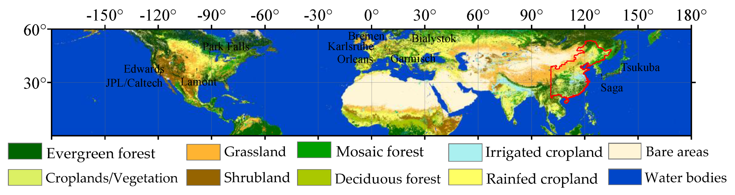
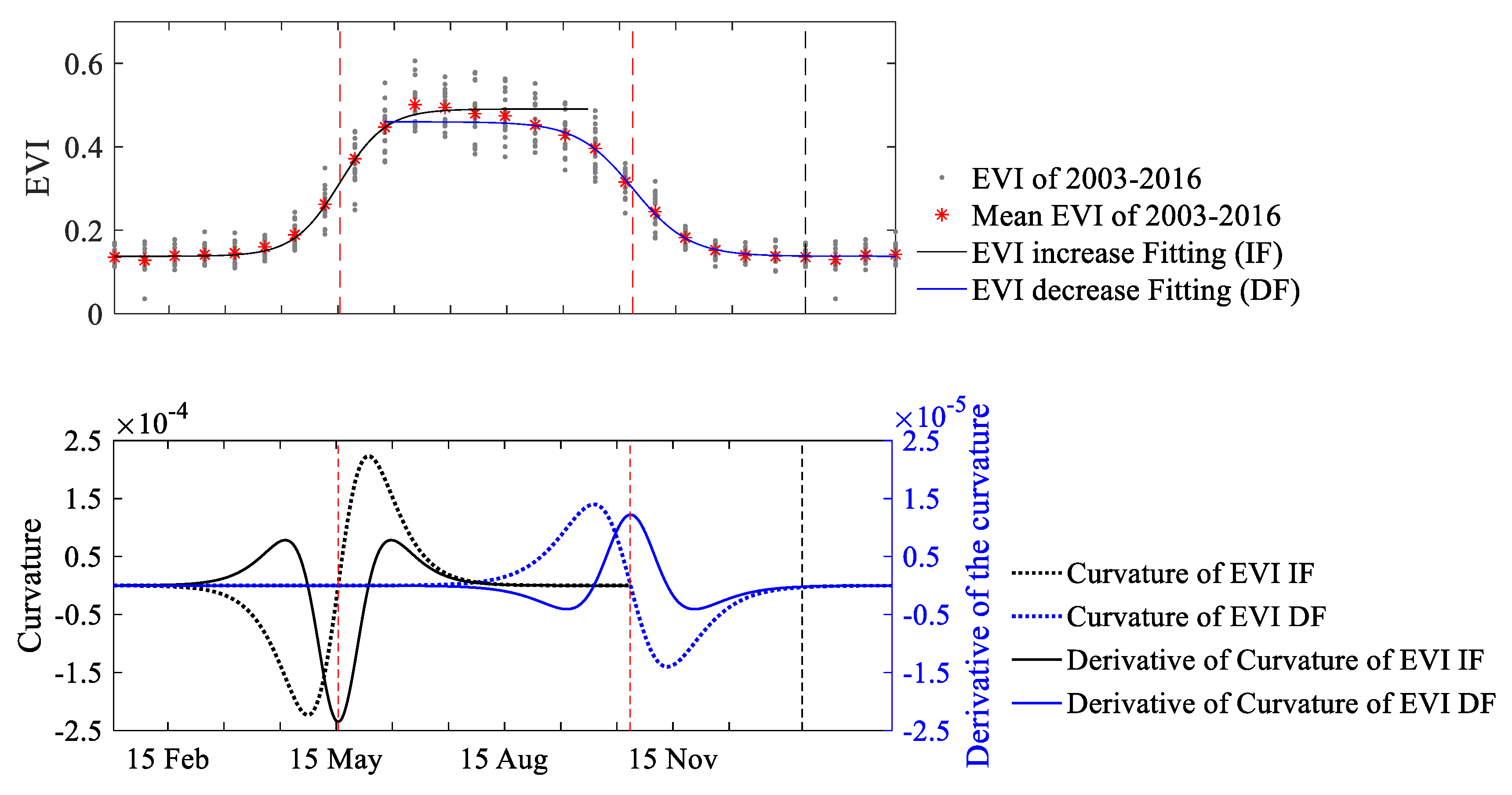
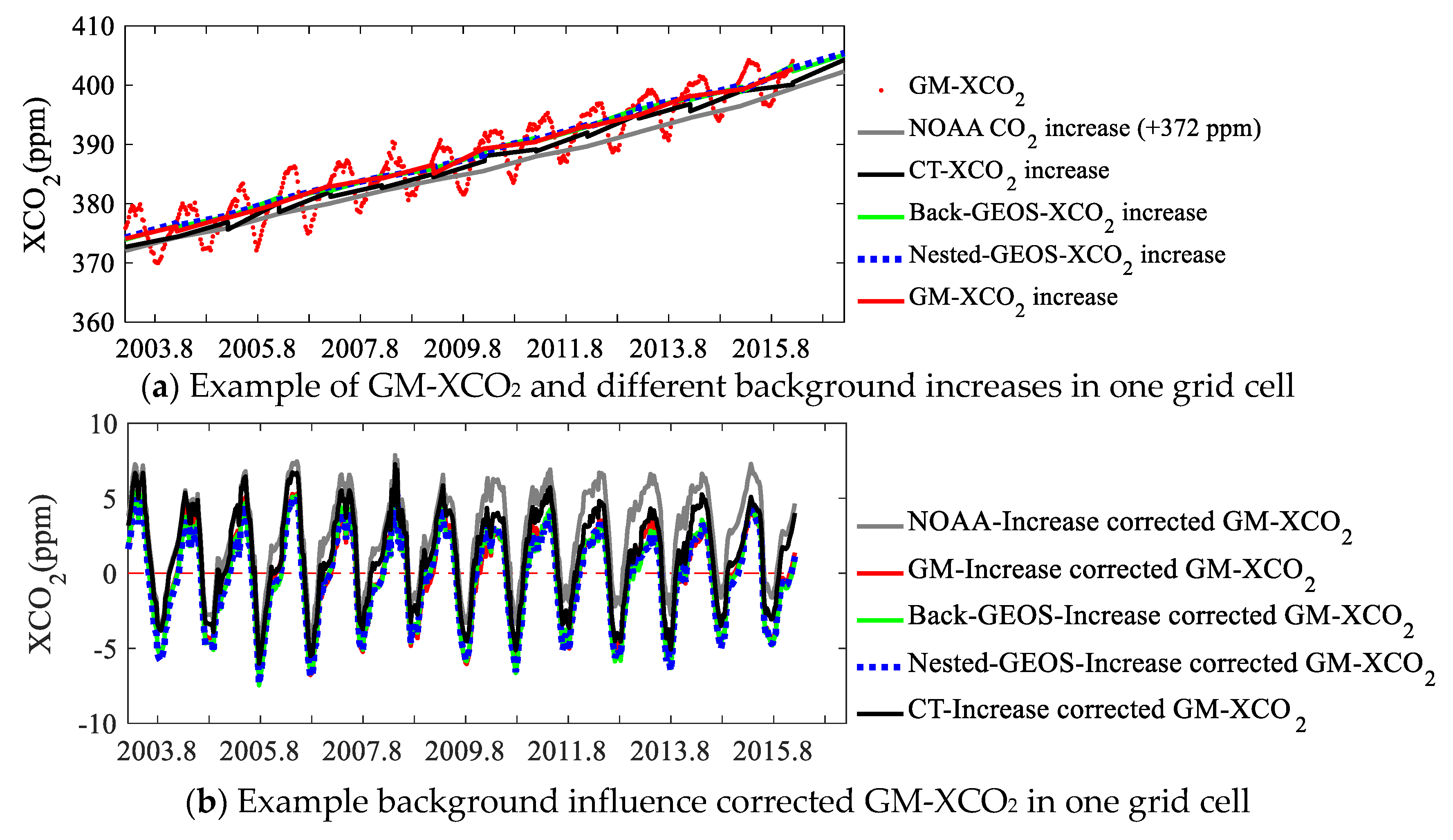
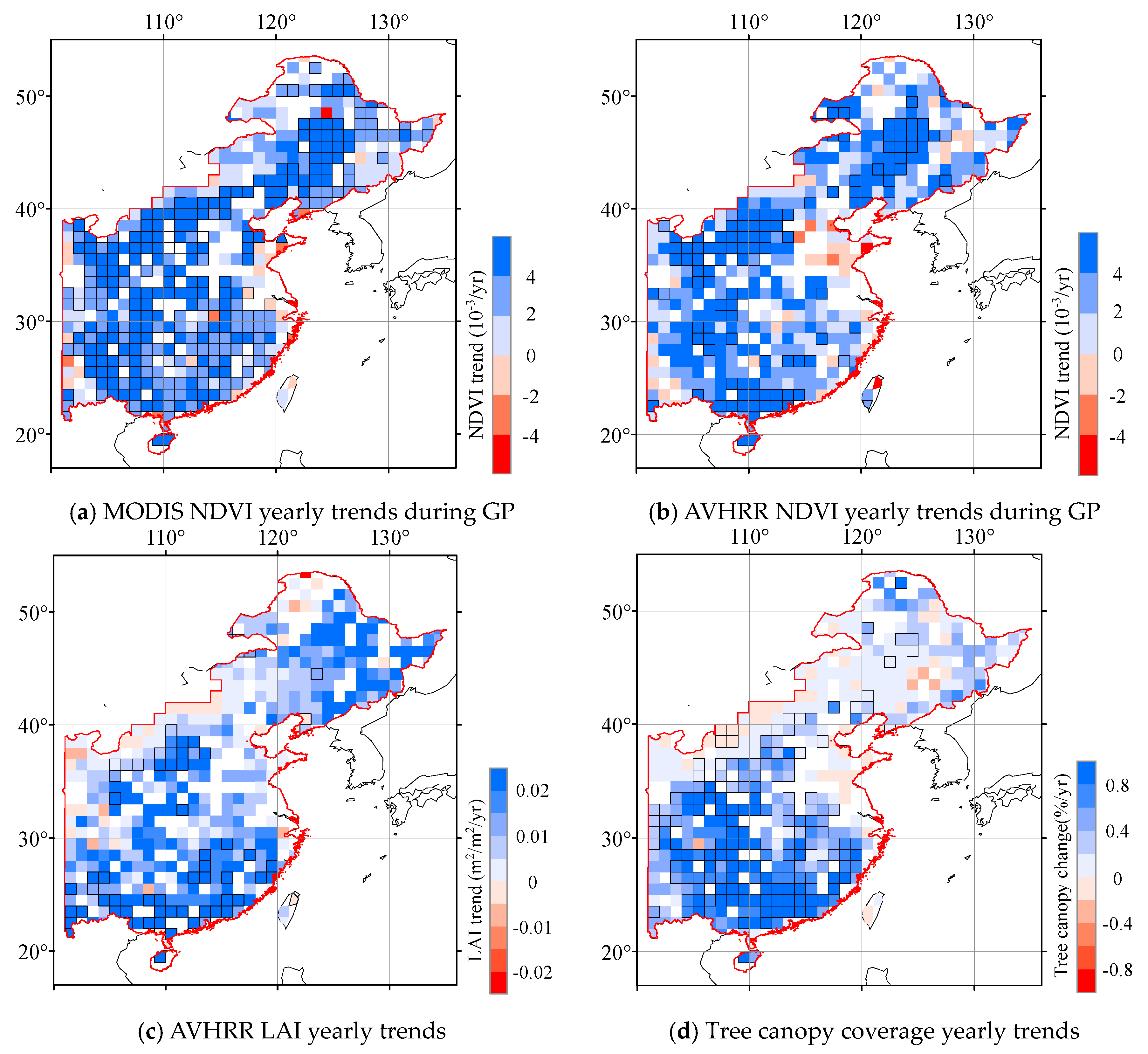
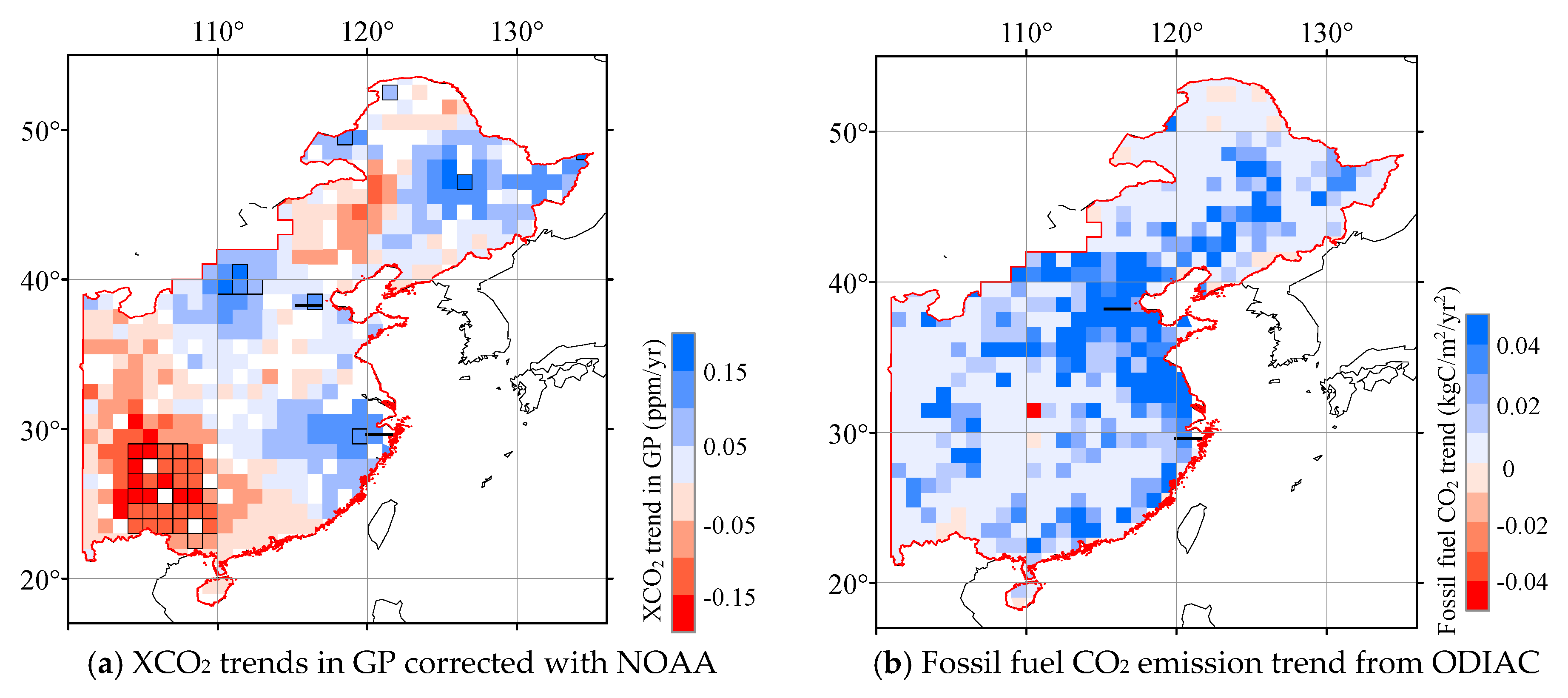
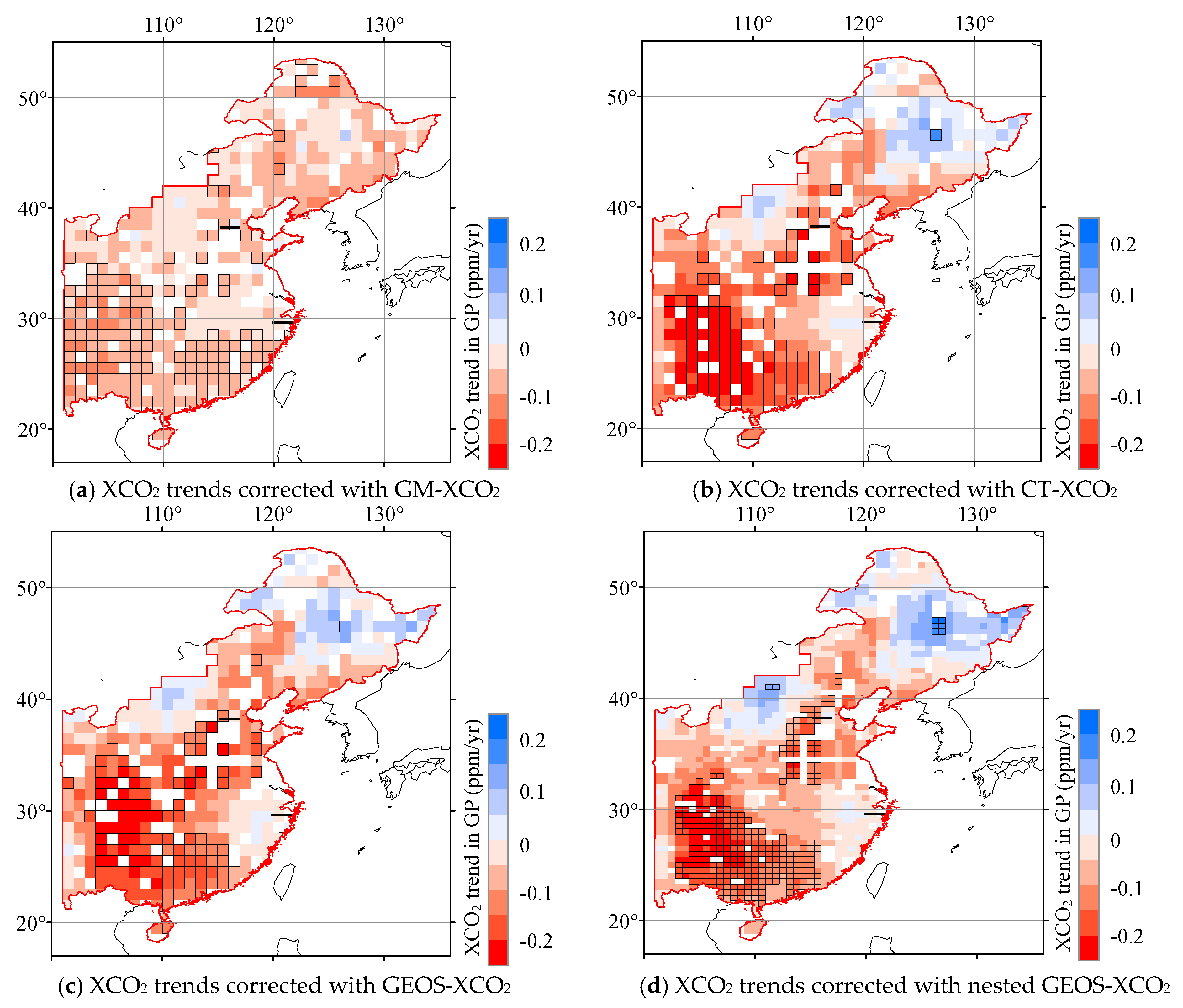
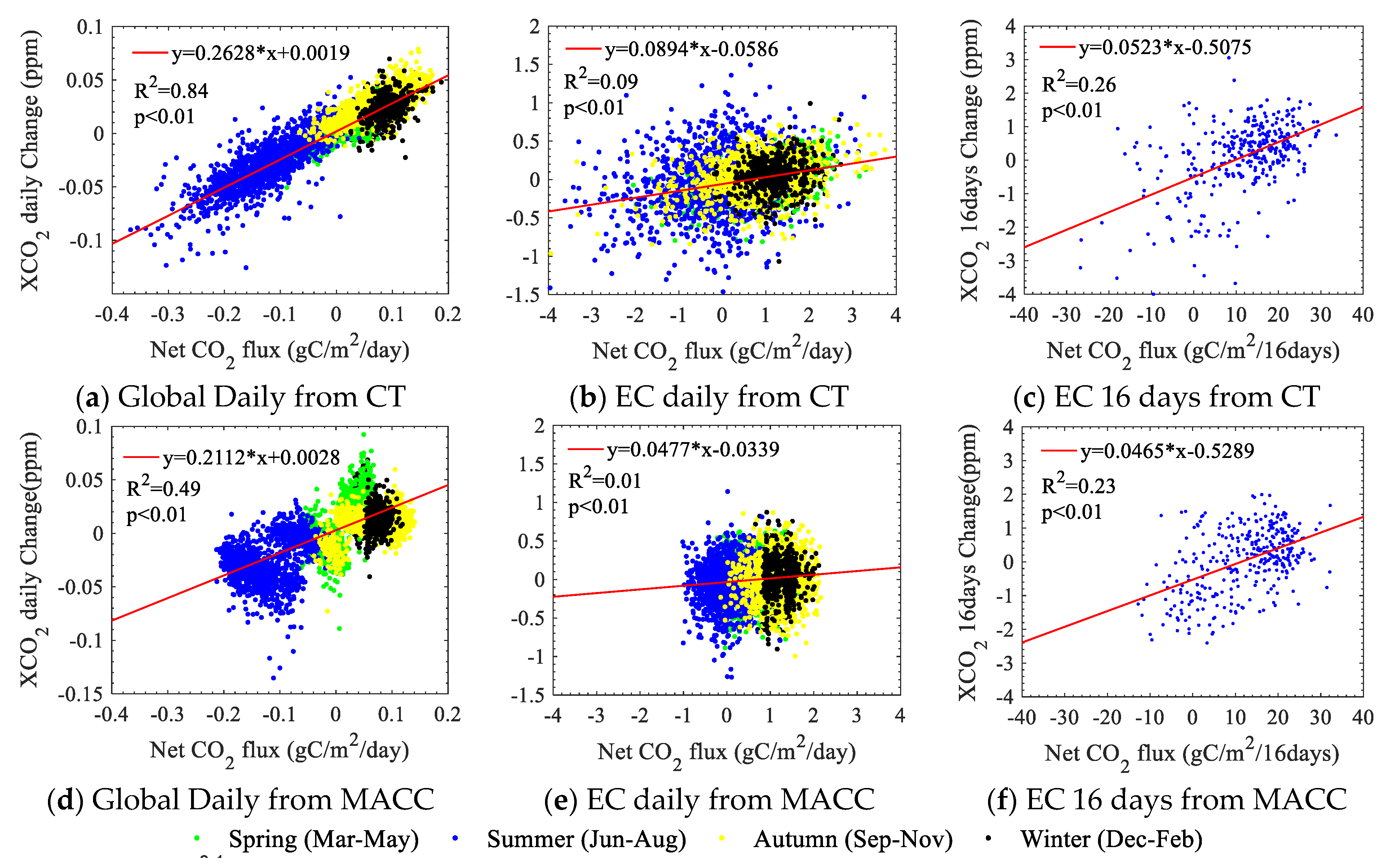
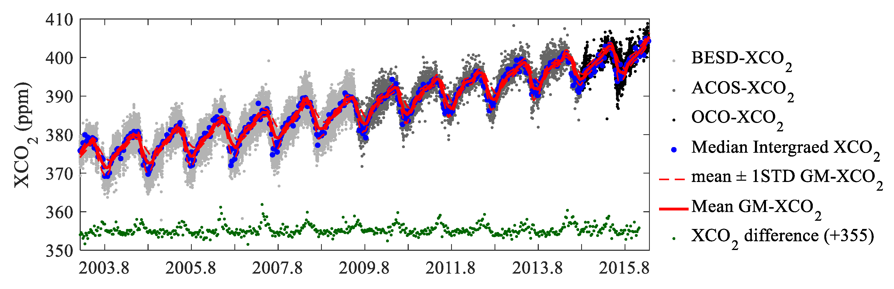
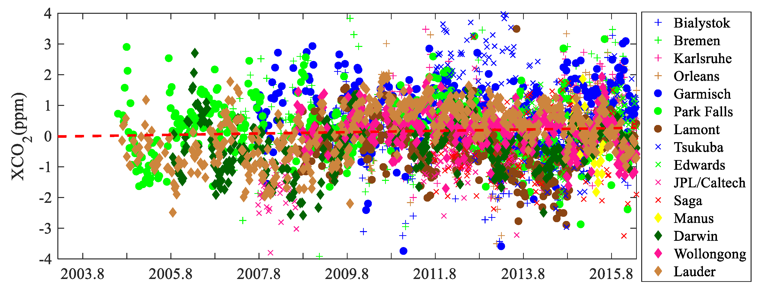
Table 1.
Datasets used in this study.
| Name | Sources | Time Res. | Space Res. | Period | Reference |
|---|---|---|---|---|---|
| NDVI/EVI | MOD13C1 v6 | 16 days | 0.05 deg. | 2003.01–2016.12 | [38] |
| NDVI | GIMMS 3g | 15 days | 1/12 deg. | [39] | |
| LAI | MCD15A3H v6 | 4 days | 500 m | [40] | |
| LAI | NOAA CDR v4 | 1 day | 0.05 deg. | [41] | |
| GPP | MOD17A2H v6 | 8 days | 500 m | [42] | |
| Global maps of XCO2 | SCIAMACHY BESD-XCO2 GOSAT ACOS-XCO2 OCO-2 XCO2 | 8 days | 1 deg. | 2003.01–2009.05 2009.06–2014.08 2014.09–2016.05 | [43,44] [45] [46] |
| XCO2/CO2 flux | CarbonTracker 2017 | 3 h | 2 × 3/1 × 1 deg. | 2003.01–2016.12 | [47] |
| XCO2/CO2 flux | MACC-III | 3 h | 1.875 × 3.75 deg. | [48] | |
| XCO2 | GEOS-Chem v11.4 | 3 h | 2 × 2.5/0.5 × 0.625 deg. | [49] | |
| TCCP | AVHRR VCF | Yearly | 0.05 deg | 2003.01–2016.12 | [50] |
| Fossil fuel CO2 Emission | ODIAC 2017 | monthly | 1 deg. | [51] | |
| LST | MCD11C2 v6 | 8 days | 0.05 deg. | [52] | |
| Precipitation | TRMM 3B42 | 3 h | 0.25 deg. | [53] |
Table 2.
GM-XCO2 decreasing trends and estimated CO2 uptake changes from 2003 to 2015 during the vegetation growing period over Eastern China (EC). There are results from three different XCO2 background corrections and two flux-XCO2 transform ratios. XCO2 background corrections are shown in Section 3.2. Transform ratios are shown in Figure 7. Uncertainties in XCO2 trends and changes refer to 1 standard deviation of spatial grid-scale variability in EC.
| Attributes\Corrections | CT-XCO2 | Back-GEOS-XCO2 | Nested-GEOS-XCO2 | |||
| XCO2 trends (ppm/yr) | −0.084 ± 0.090 | −0.081 ± 0.088 | −0.07 ± 0.093 | |||
| XCO2 change (ppm) | −1.008 ± 1.080 | −0.972 ± 1.056 | −0.840 ± 1.116 | |||
| Transform ratios | CT | MACC | CT | MACC | CT | MACC |
| Carbon uptake increase (g C/m2) | 9.57 ± 10.94 | 10.30 ±11.85 | 8.88 ± 10.48 | 9.52 ± 11.33 | 6.36 ± 11.63 | 6.69 ± 12.62 |
| Carbon amount (Tg C) | 42.76 | 46.04 | 39.69 | 42.58 | 28.41 | 29.89 |
Table 3.
Comparison of the estimated carbon uptake increase (6.36 to 10.30 g C m−2) due to greening with various posterior CO2 fluxes inferred from CT 2017 for the region during the growing period (GP) and the whole year. Posterior CO2 fluxes include the net flux, biosphere (Bio) flux, and fossil fuel emissions of annual mean and inter-annual variation. Negative values indicate carbon uptake and positive values indicate carbon emission. Values in parentheses compare the CO2 sink enhancement as percentages of the various GP CT CO2 fluxes.
| Period | Net Flux (g C m−2 yr−1) | Bio Flux (g C m−2 yr−1) | Fossil Flux (g C m−2 yr−1) |
|---|---|---|---|
| GP | 28.0 ± 54.5 | −99.8 ± 30.6 | 125.7 ± 34.8 |
| (22.6% to 36.7%) | (6.4% to 10.3%) | (5.1% to 8.2%) | |
| Annual | 264.15 ± 109.85 | −70.77 ± 36.76 | 328.48 ± 91.38 |
| (2.4% to 3.9%) | (9.0% to 14.6%) | (1.9% to 3.1%) |
© 2020 by the authors. Licensee MDPI, Basel, Switzerland. This article is an open access article distributed under the terms and conditions of the Creative Commons Attribution (CC BY) license (http://creativecommons.org/licenses/by/4.0/).
Share and Cite
MDPI and ACS Style
He, Z.; Lei, L.; Zeng, Z.-C.; Sheng, M.; Welp, L.R. Evidence of Carbon Uptake Associated with Vegetation Greening Trends in Eastern China. Remote Sens. 2020, 12, 718. https://0-doi-org.brum.beds.ac.uk/10.3390/rs12040718
AMA Style
He Z, Lei L, Zeng Z-C, Sheng M, Welp LR. Evidence of Carbon Uptake Associated with Vegetation Greening Trends in Eastern China. Remote Sensing. 2020; 12(4):718. https://0-doi-org.brum.beds.ac.uk/10.3390/rs12040718
Chicago/Turabian StyleHe, Zhonghua, Liping Lei, Zhao-Cheng Zeng, Mengya Sheng, and Lisa R. Welp. 2020. "Evidence of Carbon Uptake Associated with Vegetation Greening Trends in Eastern China" Remote Sensing 12, no. 4: 718. https://0-doi-org.brum.beds.ac.uk/10.3390/rs12040718
Note that from the first issue of 2016, this journal uses article numbers instead of page numbers. See further details here.