The Current Configuration of the OSTIA System for Operational Production of Foundation Sea Surface Temperature and Ice Concentration Analyses

 , , , , , ,
Abstract
:
1. Introduction
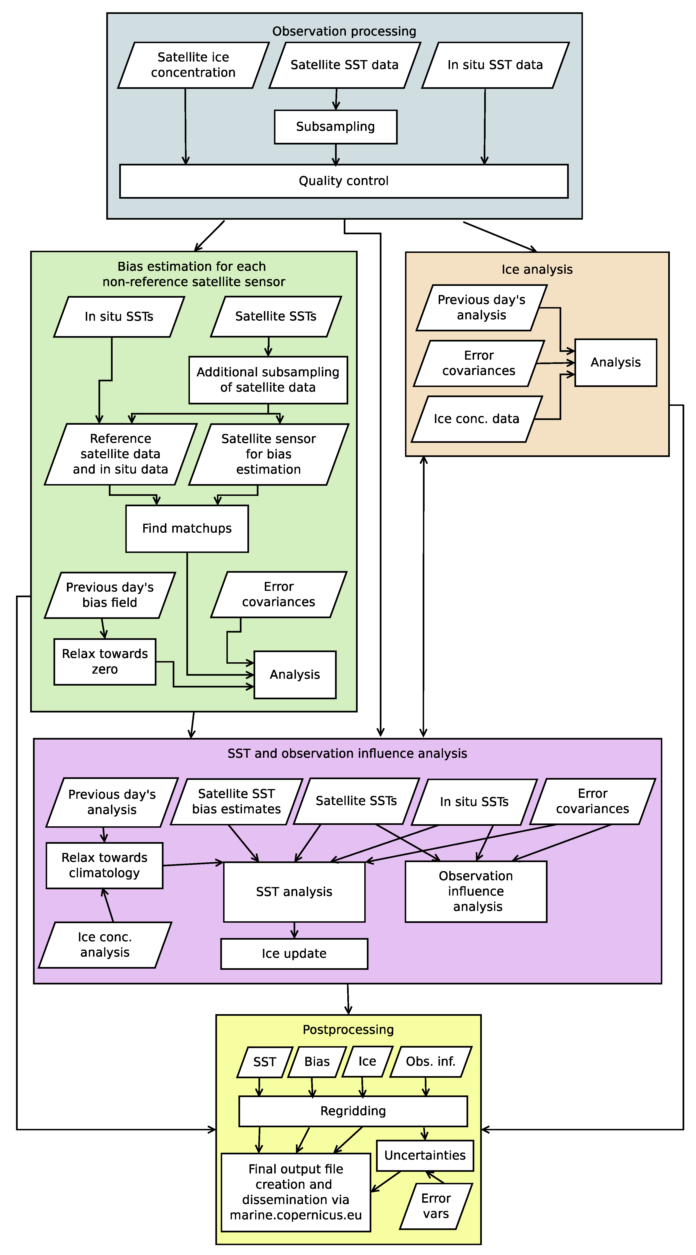
2. Methods
2.1. Observation Processing
2.1.1. Data Sources
2.1.2. Satellite SST Data Processing
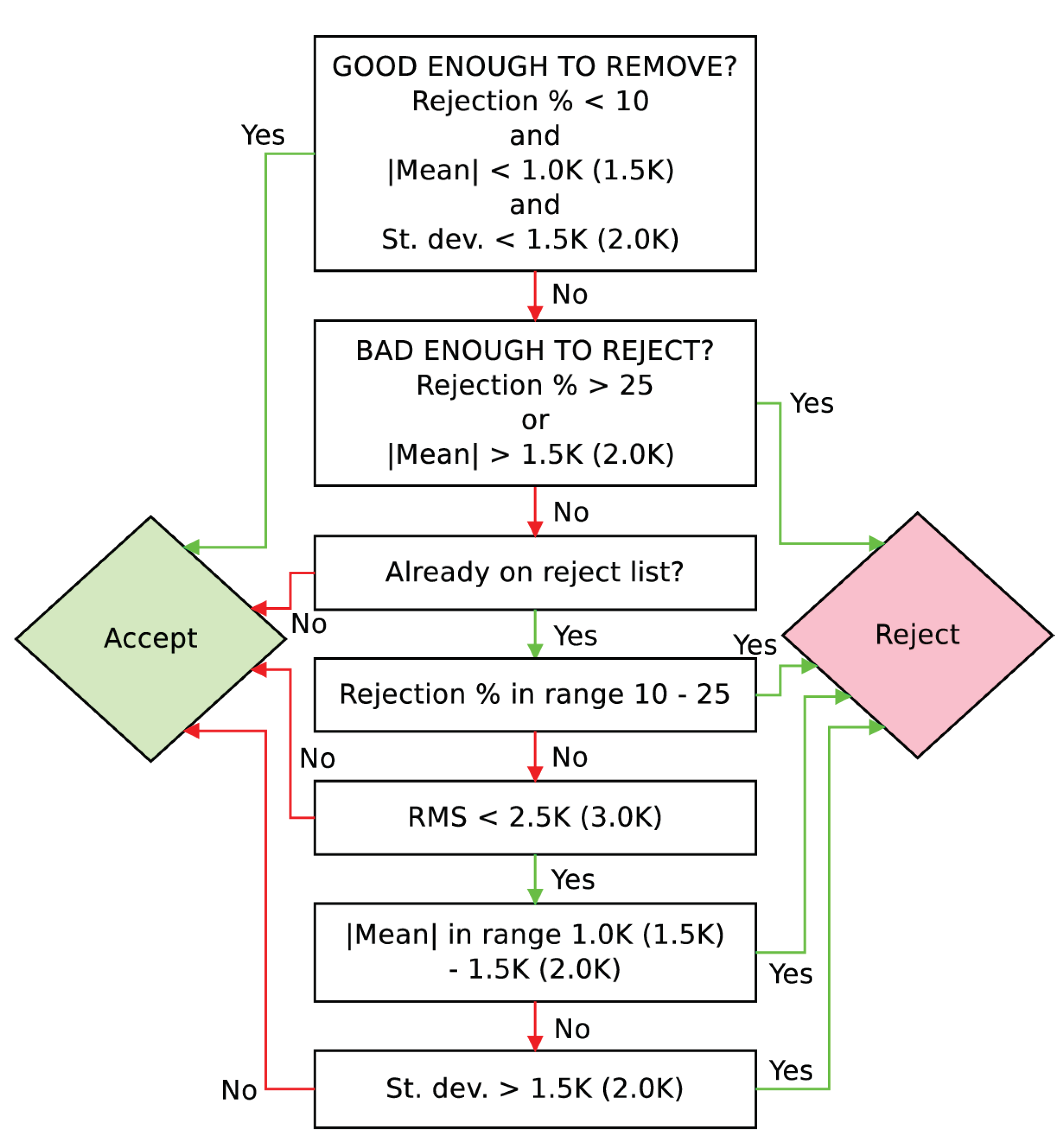
2.1.3. Quality Control
2.2. Sea Ice Analysis
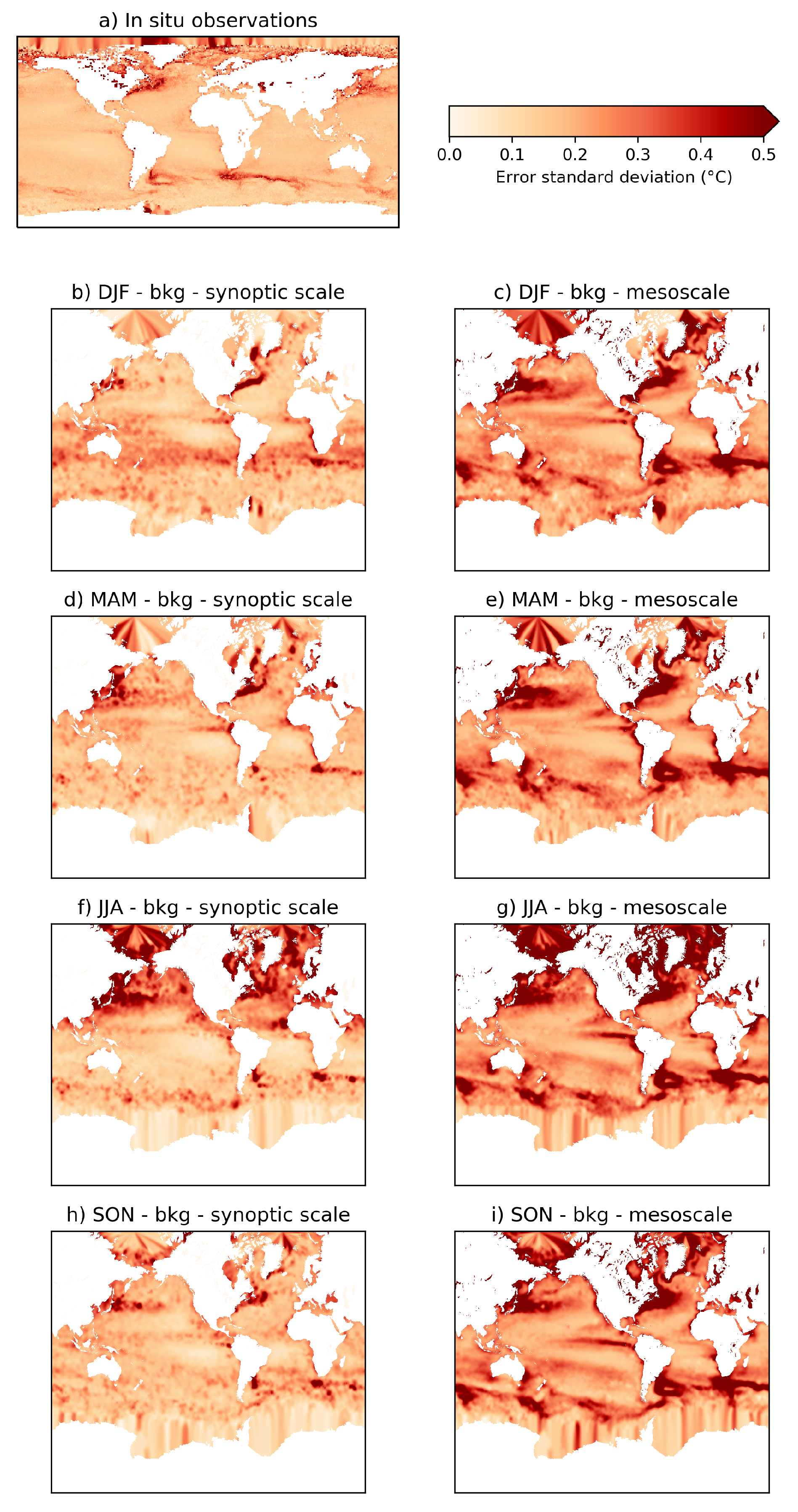
2.3. Satellite SST Bias Estimation
2.4. Analyses of SST Data
2.4.1. Temperature Analysis
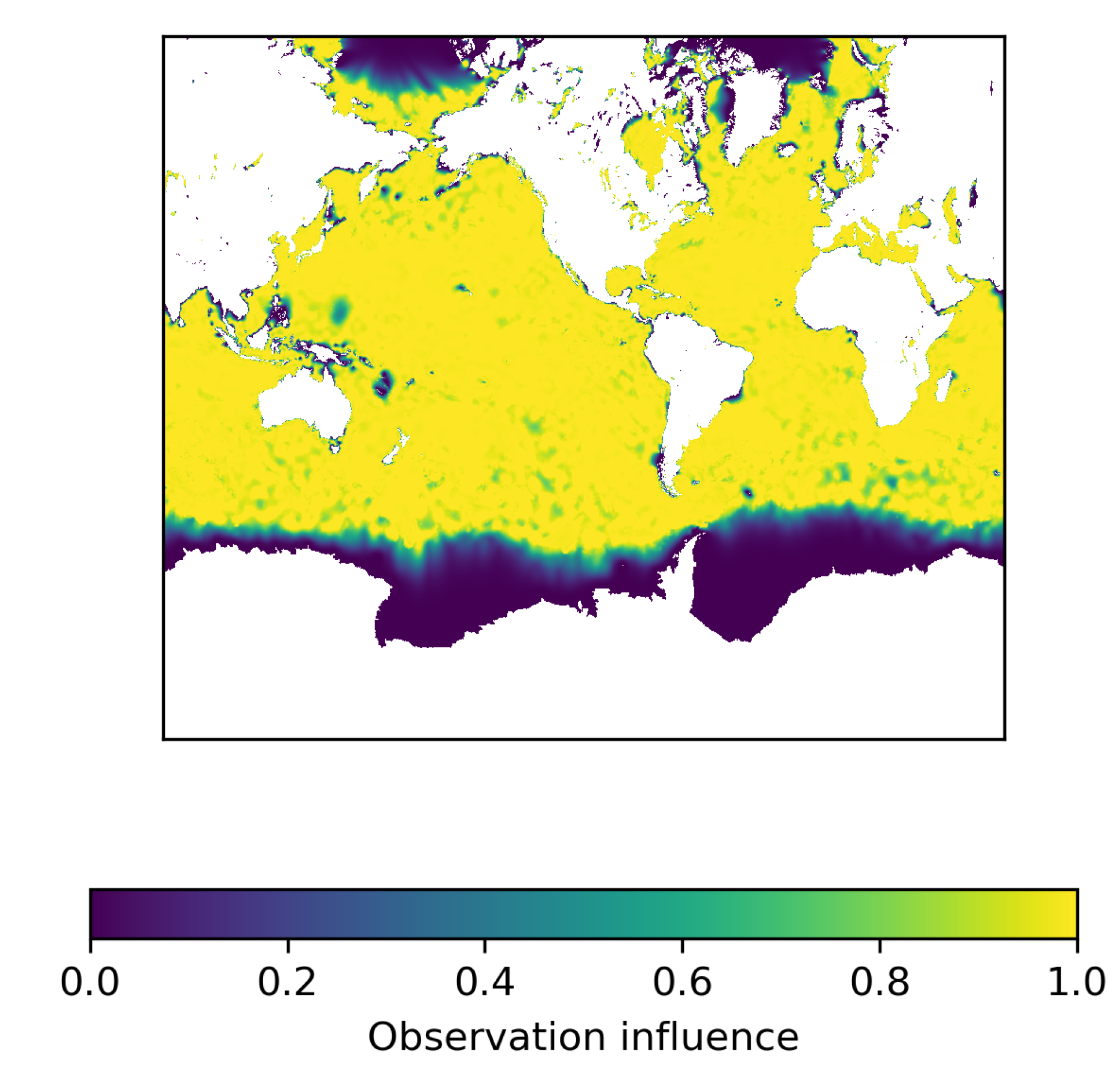
2.4.2. Observation Influence Analysis
2.5. Postprocessing
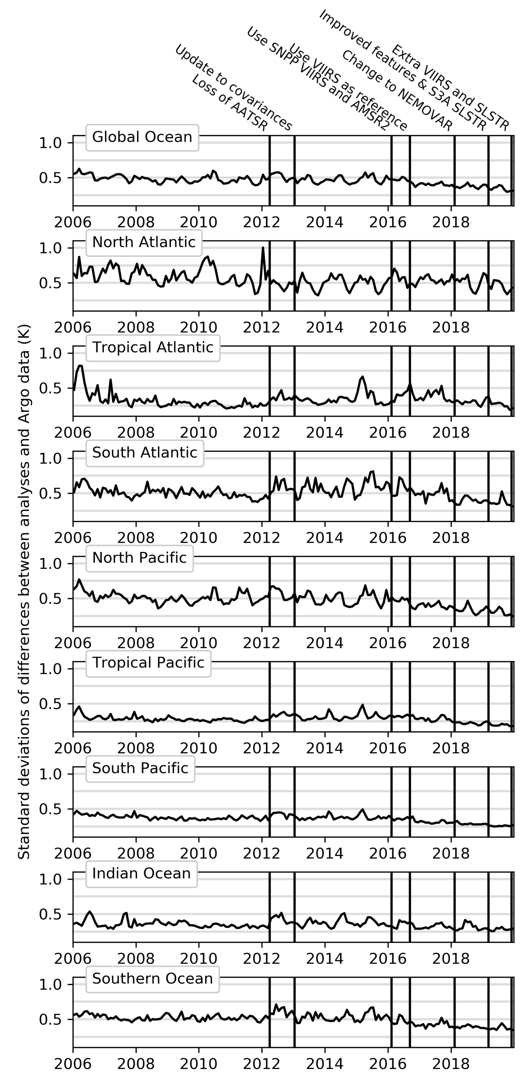
3. Results
4. Discussion
5. Conclusions
Author Contributions
Funding
Acknowledgments
Conflicts of Interest
Abbreviations
| AMSR | Advanced Microwave Scanning Radiometer |
| AVHRR | Advanced Very High Resolution Radiometer |
| CDR | Climate Data Record |
| DMSP | Defense Meteorological Satellite Program |
| EUMETSAT | European Organisation for the Exploitation of Meteorological Satellites |
| GCOM-W | Global Change Observation Mission - Water |
| GHRSST | Group for High Resolution SST |
| L2P | Level 2 Preprocessed |
| L3U | Level 3 Uncollated |
| L3C | Level 3 Collated |
| MetOp-B | Meteorological operational satellite B |
| MSG | Meteosat Second Generation |
| NAVO | Naval Oceanographic Office |
| NCEP | National Centers for Environmental Prediction |
| NOAA | National Oceanographic and Atmospheric Administration |
| OSI SAF | Ocean and Sea Ice Satellite Application Facility |
| OSPO | Office of Satellite and Product Operations |
| REMSS | Remote Sensing Systems |
| SEVIRI | Spinning Enhanced Visible Infra-Red Imager |
| SLSTR | Sea and Land Surface Temperature Radiometer |
| SNPP | Suomi National Polar-orbiting Partnership |
| SSMI/S | Special Sensor Microwave Imager / Sounder |
| SST | Sea Surface Temperature |
| WMO | World Meteorological Organisation |
| VIIRS | Visible/Infrared Imager Radiometer Suite |
References
- Donlon, C.J.; Martin, M.; Stark, J.; Roberts-Jones, J.; Fiedler, E.; Wimmer, W. The Operational Sea Surface Temperature and Sea Ice Analysis (OSTIA) system. Remote Sens. Environ. 2012, 116, 140–158. [Google Scholar] [CrossRef]
- Balmaseda, M.A.; Mogensen, K.; Weaver, A.T. Evaluation of the ECMWF ocean reanalysis system ORAS4. Q. J. R. Meteorol. Soc. 2013, 139, 1132–1161. [Google Scholar] [CrossRef]
- Dee, D.P.; Uppala, S.M.; Simmons, A.J.; Berrisford, P.; Poli, P.; Kobayashi, S.; Andrae, U.; Balmaseda, M.A.; Balsamo, G.; Bauer, P.; et al. The ERA-Interim reanalysis: Configuration and performance of the data assimilation system. Q. J. R. Meteorol. Soc. 2011, 137, 553–597. [Google Scholar] [CrossRef]
- Petch, J.C.; Short, C.J.; Best, M.J.; McCarthy, M.; Lewis, H.W.; Vosper, S.B.; Weeks, M. Sensitivity of the 2018 UK summer heatwave to local sea temperatures and soil moisture. Atmos. Sci. Lett. 2020, e948. [Google Scholar] [CrossRef] [Green Version]
- Schneemann, J.; Rott, A.; Dörenkämper, M.; Steinfeld, G.; Kühn, M. Cluster wakes impact on a far-distant offshore wind farm’s power. Wind Energy Sci. 2020, 5, 29–49. [Google Scholar] [CrossRef] [Green Version]
- Roberts-Jones, J.; Fiedler, E.K.; Martin, M.J. Daily, Global, High-Resolution SST and Sea Ice Reanalysis for 1985–2007 Using the OSTIA System. J. Clim. 2012, 25, 6215–6232. [Google Scholar] [CrossRef]
- Merchant, C.J.; Embury, O.; Roberts-Jones, J.; Fiedler, E.; Bulgin, C.E.; Corlett, G.K.; Good, S.; McLaren, A.; Rayner, N.; Morak-Bozzo, S.; et al. Sea surface temperature datasets for climate applications from Phase 1 of the European Space Agency Climate Change Initiative (SST CCI). Geosci. Data J. 2014, 1, 179–191. [Google Scholar] [CrossRef] [Green Version]
- Merchant, C.J.; Embury, O.; Bulgin, C.E.; Block, T.; Corlett, G.K.; Fiedler, E.; Good, S.A.; Mittaz, J.; Rayner, N.A.; Berry, D.; et al. Satellite-based time-series of sea-surface temperature since 1981 for climate applications. Sci. Data 2019, 6. [Google Scholar] [CrossRef] [PubMed] [Green Version]
- While, J.; Mao, C.; Martin, M.J.; Roberts-Jones, J.; Sykes, P.A.; Good, S.A.; McLaren, A.J. An operational analysis system for the global diurnal cycle of sea surface temperature: Implementation and validation. Q. J. R. Meteorol. Soc. 2017, 143, 1787–1803. [Google Scholar] [CrossRef]
- Lorenc, A.C.; Bell, R.S.; Macpherson, B. The Meteorological Office analysis correction data assimilation scheme. Q. J. R. Meteorol. Soc. 1991, 117, 59–89. [Google Scholar] [CrossRef]
- Martin, M.J.; Hines, A.; Bell, M.J. Data assimilation in the FOAM operational short-range ocean forecasting system: A description of the scheme and its impact. Q. J. R. Meteorol. Soc. 2007, 133, 981–995. [Google Scholar] [CrossRef]
- Mogensen, K.; Alonso-Balmaseda, M.; Weaver, A.; Martin, M.; Vidard, A. NEMOVAR: A variational data assimilation system for the NEMO ocean model. ECMWF Newsl. 2009, 120, 17–21. [Google Scholar] [CrossRef]
- Madec, G.; Bourdallé-Badie, R.; Bouttier, P.A.; Bricaud, C.; Bruciaferri, D.; Calvert, D.; Chanut, J.; Clementi, E.; Coward, A.; Delrosso, D.; et al. NEMO ocean engine. Notes du Pôle de Modélisation de lÍnstitut Pierre-Simon Laplace (IPSL) 2017. [Google Scholar] [CrossRef]
- Waters, J.; Lea, D.J.; Martin, M.J.; Mirouze, I.; Weaver, A.; While, J. Implementing a variational data assimilation system in an operational 1/4 degree global ocean model. Q. J. R. Meteorol. Soc. 2015, 141, 333–349. [Google Scholar] [CrossRef]
- Fiedler, E.K.; Martin, M.J.; Roberts-Jones, J. An operational analysis of Lake Surface Water Temperature. Tellus A Dyn. Meteorol. Oceanogr. 2014, 66, 21247. [Google Scholar] [CrossRef] [Green Version]
- Roberts-Jones, J.; Bovis, K.; Martin, M.J.; McLaren, A. Estimating background error covariance parameters and assessing their impact in the OSTIA system. Remote Sens. Environ. 2016, 176, 117–138. [Google Scholar] [CrossRef]
- Fiedler, E.K.; Mao, C.; Good, S.A.; Waters, J.; Martin, M.J. Improvements to feature resolution in the OSTIA sea surface temperature analysis using the NEMOVAR assimilation scheme. Q. J. R. Meteorol. Soc. 2019, 145, 3609–3625. [Google Scholar] [CrossRef]
- GHRSST Science Team. The Recommended GHRSST Data Specification (GDS) 2.0, Document Revision 4 (2010); GHRSST International Project Office: Leicester, UK, 2011. [Google Scholar]
- Wentz, F.; Meissner, T.; Gentemann, C.; Hilburn, K.; Scott, J. Remote Sensing Systems GCOM-W1 AMSR2 Daily) Environmental Suite on 0.25 deg grid, Version 8a. Remote Sensing Systems, Santa Rosa, CA. Available online: www.remss.com/missions/amsr (accessed on 30 December 2019).
- REMSS. Remote Sensing Systems GHRSST Level 2P Global Subskin Sea Surface Temperature version 8a from the Advanced Microwave Scanning Radiometer 2 on the GCOM-W satellite. Ver. 8a. PO.DAAC, CA, USA. Available online: https://0-doi-org.brum.beds.ac.uk/10.5067/GHAM2-2PR8A (accessed on 30 December 2019).
- Petrenko, B.; Ignatov, A.; Kihai, Y.; Stroup, J.; Dash, P. Evaluation and selection of SST regression algorithms for JPSS VIIRS. J. Geophys. Res. Atmos. 2014, 119, 4580–4599. [Google Scholar] [CrossRef]
- NOAA OSPO. Office of Satellite arnd Product Operations GHRSST Level 3U OSPO dataset v2.61 from VIIRS on NOAA-20 Satellite (GDS v2). Ver. 2.61. PO.DAAC, CA, USA. Available online: https://0-doi-org.brum.beds.ac.uk/10.5067/GHV20-3UO61 (accessed on 30 December 2019).
- Donlon, C.J.; Nightingale, T.J.; Sheasby, T.; Turner, J.; Robinson, I.S.; Emergy, W.J. Implications of the oceanic thermal skin temperature deviation at high wind speed. Geophys. Res. Lett. 1999, 26, 2505–2508. [Google Scholar] [CrossRef]
- Donlon, C.J.; Minnett, P.J.; Gentemann, C.; Nightingale, T.J.; Barton, I.J.; Ward, B.; Murray, M.J. Toward Improved Validation of Satellite Sea Surface Skin Temperature Measurements for Climate Research. J. Clim. 2002, 15, 353–369. [Google Scholar] [CrossRef] [Green Version]
- Lorenc, A.C.; Hammon, O. Objective quality control of observations using Bayesian methods. Theory, and a practical implementation. Q. J. R. Meteorol. Soc. 1988, 114, 515–543. [Google Scholar] [CrossRef]
- Ingleby, B.; Huddleston, M. Quality control of ocean temperature and salinity profiles - Historical and real-time data. J. Mar. Syst. 2007, 65, 158–175. [Google Scholar] [CrossRef]
- Storkey, D.; Blaker, A.T.; Mathiot, P.; Megann, A.; Aksenov, Y.; Blockley, E.W.; Calvert, D.; Graham, T.; Hewitt, H.T.; Hyder, P.; et al. UK Global Ocean GO6 and GO7: A traceable hierarchy of model resolutions. Geosci. Model Dev. 2018, 11, 3187–3213. [Google Scholar] [CrossRef] [Green Version]
- Steele, M.; Morley, R.; Ermold, W. PHC: A Global Ocean Hydrography with a High-Quality Arctic Ocean. J. Clim. 2001, 14, 2079–2087. [Google Scholar] [CrossRef]
- Fofonoff, N.; Millard, R., Jr. Algorithms for the computation of fundamental properties of seawater. In UNESCO Technical Papers in Marine Sciences 44; UNESCO: Paris, France, 1983. [Google Scholar]
- Mirouze, I.; Blockley, E.W.; Lea, D.J.; Martin, M.J.; Bell, M.J. A multiple length scale correlation operator for ocean data assimilation. Tellus A Dyn. Meteorol. Oceanogr. 2016, 68, 29744. [Google Scholar] [CrossRef] [Green Version]
- Casey, K.S.; Brandon, T.B.; Cornillon, P.; Evans, R. The Past, Present, and Future of the AVHRR Pathfinder SST Program. In Oceanography from Space: Revisited; Barale, V., Gower, J., Alberotanza, L., Eds.; Springer: Dordrecht, The Netherlands, 2010; pp. 273–287. [Google Scholar] [CrossRef]
- Argo Float Data and Metadata from Global Data Assembly Centre (Argo GDAC); SEANOE: Paris, France, 2020. [CrossRef]
- Good, S.A.; Martin, M.J.; Rayner, N.A. EN4: Quality controlled ocean temperature and salinity profiles and monthly objective analyses with uncertainty estimates. J. Geophys. Res. Ocean. 2013, 118, 6704–6716. [Google Scholar] [CrossRef]
- Fiedler, E.K.; McLaren, A.; Banzon, V.; Brasnett, B.; Ishizaki, S.; Kennedy, J.; Rayner, N.; Roberts-Jones, J.; Corlett, G.; Merchant, C.J.; et al. Intercomparison of long-term sea surface temperature analyses using the GHRSST Multi-Product Ensemble (GMPE) system. Remote Sens. Environ. 2019, 222, 18–33. [Google Scholar] [CrossRef] [Green Version]
- Dash, P.; Ignatov, A.; Kihai, Y.; Sapper, J. The SST Quality Monitor (SQUAM). J. Atmos. Ocean. Technol. 2010, 27, 1899–1917. [Google Scholar] [CrossRef]
- Dash, P.; Ignatov, A.; Martin, M.; Donlon, C.; Brasnett, B.; Reynolds, R.W.; Banzon, V.; Beggs, H.; Cayula, J.F.; Chao, Y.; et al. Group for High Resolution Sea Surface Temperature (GHRSST) analysis fields inter-comparisons—Part 2: Near real time web-based level 4 SST Quality Monitor (L4-SQUAM). Deep. Sea Res. Part II Top. Stud. Oceanogr. 2012, 77–80, 31–43. [Google Scholar] [CrossRef] [Green Version]
- Martin, M.; Dash, P.; Ignatov, A.; Banzon, V.; Beggs, H.; Brasnett, B.; Cayula, J.F.; Cummings, J.; Donlon, C.; Gentemann, C.; et al. Group for High Resolution Sea Surface temperature (GHRSST) analysis fields inter-comparisons. Part 1: A GHRSST multi-product ensemble (GMPE). Deep. Sea Res. Part II Top. Stud. Oceanogr. 2012, 77–80, 21–30. [Google Scholar] [CrossRef]


| Instrument | Satellite | Producer | Data Level | Spatial Resolution | Thinning | References | Notes |
|---|---|---|---|---|---|---|---|
| AMSR2 | GCOM-W | REMSS | L2P | 25 km | 2 × 2 | [19,20] | |
| AVHRR | MetOp-B | OSI SAF | L2P | 1 km | 6 × 6 | OSI SAF product OSI-204-b | |
| In situ | – | Various | – | – | None | Drifting/moored buoys used in reference | |
| SEVIRI | MSG | OSI SAF | L3C | 0.05 | 6 × 6 | OSI SAF product OSI-206-a | |
| VIIRS | SNPP | NOAA OSPO | L3U | 0.02 | 6 × 6 | [21] | Used in reference |
| VIIRS | NOAA-20 | NOAA OSPO | L3U | 0.02 | 6 × 6 | [21,22] | Used in reference |
| SLSTR | Sentinel 3A | EUMETSAT | L2P | 1 km at nadir | 6 × 6 | Dual view only | |
| SLSTR | Sentinel 3B | EUMETSAT | L2P | 1 km at nadir | 6 × 6 | Dual view only |
| Variable Name | Dimensions | Notes |
|---|---|---|
| time | 1 | Nominal time that the SST analysis represents |
| lat | 3600 | Central latitudes of the grid points |
| lon | 7200 | Central longitudes of the grid points |
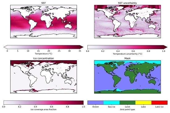
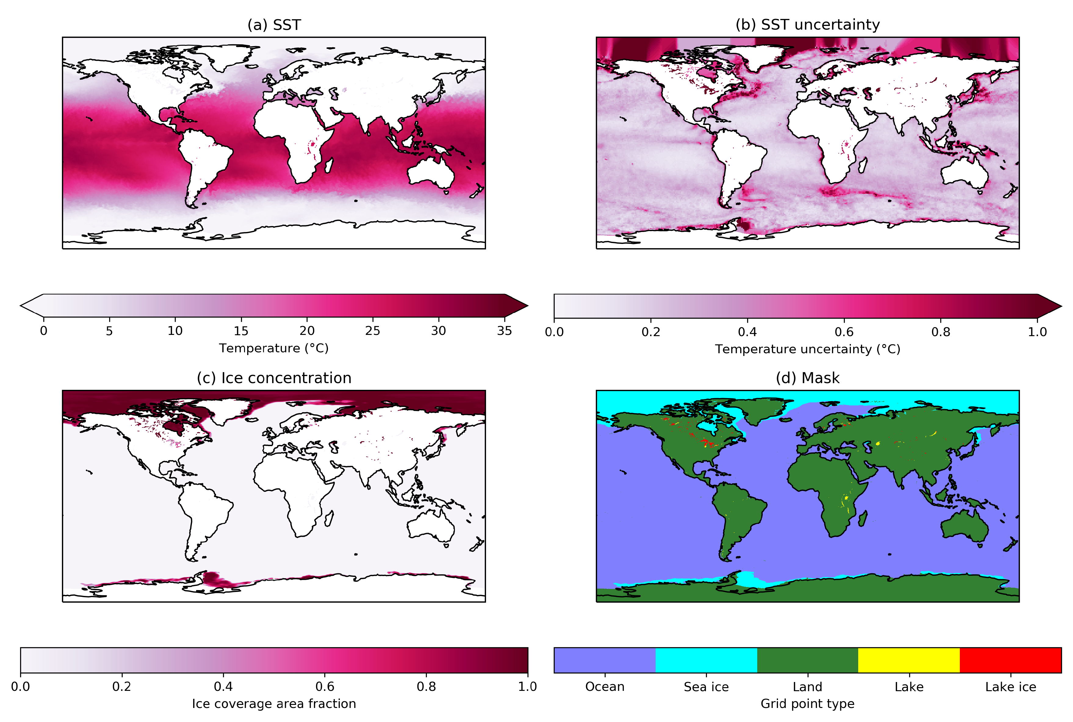
| analysed_sst | 1 × 3600 × 7200 | The SST analysis (packed data) |
| analysis_error | 1 × 3600 × 7200 | The uncertainty in the SST analysis (packed data) |
| sea_ice_fraction | 1 × 3600 × 7200 | The IC analysis (packed data) |
| mask | 1 × 3600 × 7200 | Water / land / lake / ice mask |
© 2020 by the authors. Licensee MDPI, Basel, Switzerland. This article is an open access article distributed under the terms and conditions of the Creative Commons Attribution (CC BY) license (http://creativecommons.org/licenses/by/4.0/).
Share and Cite
Good, S.; Fiedler, E.; Mao, C.; Martin, M.J.; Maycock, A.; Reid, R.; Roberts-Jones, J.; Searle, T.; Waters, J.; While, J.; et al. The Current Configuration of the OSTIA System for Operational Production of Foundation Sea Surface Temperature and Ice Concentration Analyses. Remote Sens. 2020, 12, 720. https://0-doi-org.brum.beds.ac.uk/10.3390/rs12040720
Good S, Fiedler E, Mao C, Martin MJ, Maycock A, Reid R, Roberts-Jones J, Searle T, Waters J, While J, et al. The Current Configuration of the OSTIA System for Operational Production of Foundation Sea Surface Temperature and Ice Concentration Analyses. Remote Sensing. 2020; 12(4):720. https://0-doi-org.brum.beds.ac.uk/10.3390/rs12040720
Chicago/Turabian StyleGood, Simon, Emma Fiedler, Chongyuan Mao, Matthew J. Martin, Adam Maycock, Rebecca Reid, Jonah Roberts-Jones, Toby Searle, Jennifer Waters, James While, and et al. 2020. "The Current Configuration of the OSTIA System for Operational Production of Foundation Sea Surface Temperature and Ice Concentration Analyses" Remote Sensing 12, no. 4: 720. https://0-doi-org.brum.beds.ac.uk/10.3390/rs12040720