Real-time Reconstruction of Surface Velocities from Satellite Observations in the Alboran Sea

Abstract

Surface currents in the Alboran Sea are characterized by a very fast evolution that is not well captured by altimetric maps due to sampling limitations. On the contrary, satellite infrared measurements provide high resolution synoptic images of the ocean at high temporal rate, allowing to capture the evolution of the flow. The capability of Surface Quasi-Geostrophic (SQG) dynamics to retrieve surface currents from thermal images was evaluated by comparing resulting velocities with in situ observations provided by surface drifters. A difficulty encountered comes from the lack of information about ocean salinity. We propose to exploit the strong relationship between salinity and temperature to identify water masses with distinctive salinity in satellite images and use this information to correct buoyancy. Once corrected, our results show that the SQG approach can retrieve ocean currents slightly better to that of near-real-time currents derived from altimetry in general, but much better in areas badly sampled by altimeters such as the area to the east of the Strait of Gibraltar. Although this area is far from the geostrophic equilibrium, the results show that the good sampling of infrared radiometers allows at least retrieving the direction of ocean currents in this area. The proposed approach can be used in other areas of the ocean for which water masses with distinctive salinity can be identified from satellite observations.

1. Introduction

The Strait of Gibraltar is the natural connection of the Mediterranean Sea with the world ocean, being a hot spot area in many senses. There, diverse and separated hydrodynamic phenomena occur over a wide range of spatial and temporal scales (from the small scales and submesoscale phenomena to inter-annual and climate variability). The complex hydrodynamic conditions influence the rich marine ecosystem in the adjacent coastal areas, e.g., [1,2,3]. Furthermore, the region is of great socioeconomic relevance as a key passage for marine trade. Almost 1/6 of global sea traffic and 1/5 of global oil traffic transits through the Mediterranean basin, still being the shortest route between Europe and Asia [4]. Then, it is not surprising that the Strait of Gibraltar and the adjacent Alboran Sea have been traditionally a focus area for many research and monitoring efforts since a long time ago, e.g., [5,6,7]. Although the main characteristics of the prominent processes are reasonably known and modeling efforts capture most of them, an adequate operational forecast of the hydrodynamics conditions in this region remains a challenging task [8]. Roughly, the water mass structure is close to a two-layer system characterized by an upper surface layer of Atlantic waters entering into the basin and denser Mediterranean waters outflowing below [9]. The inflow of Atlantic water and the outflow of Mediterranean water are constrained by hydraulic control in the channel where the bottom relief, stratification, tidal, and wind regimes determine the variability of water exchanges through the strait, which are therefore linked to basin scale variability, e.g., [10,11].

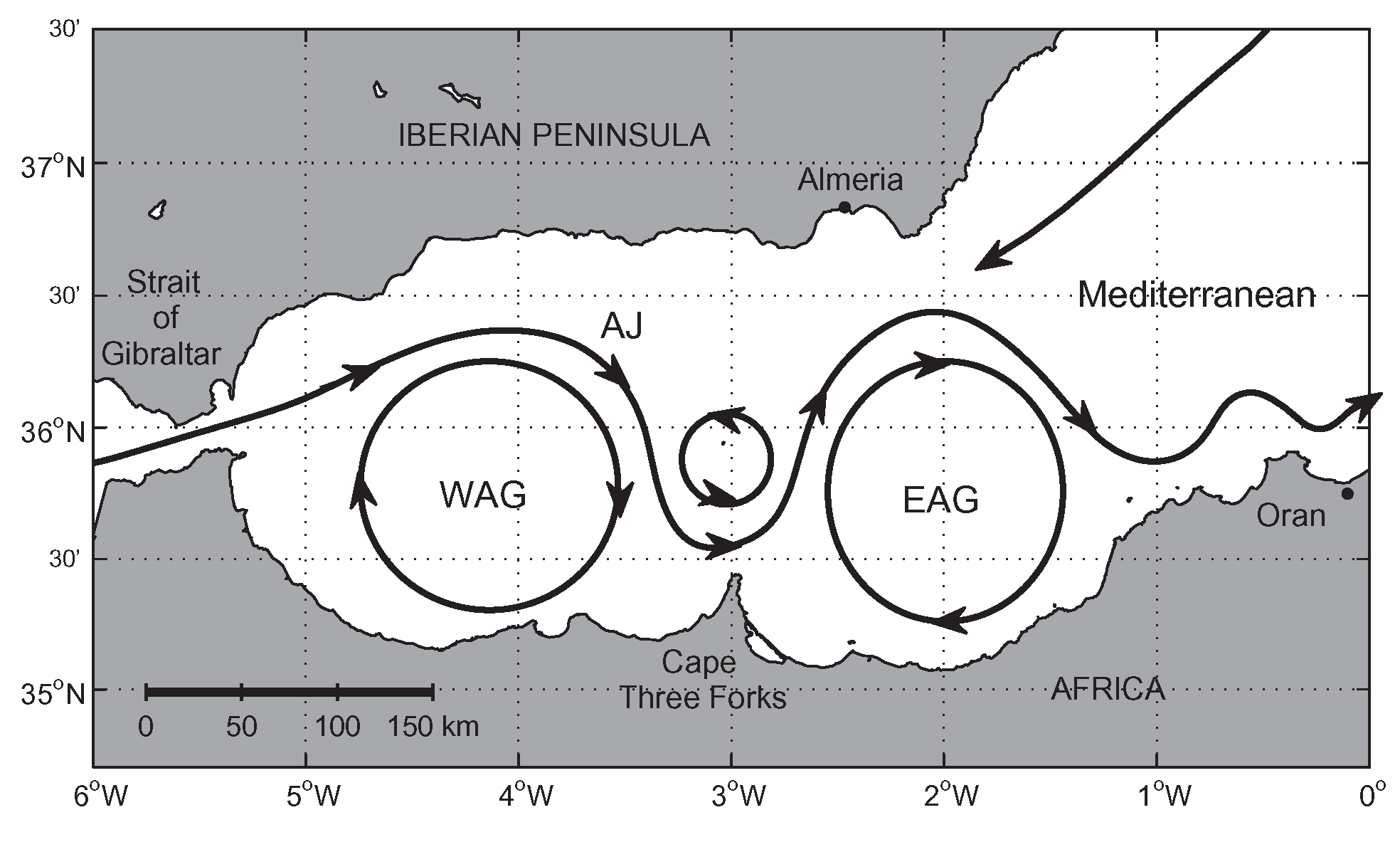
The jet of Atlantic water forms and configures a quasi-permanent vortex or gyre in the western part (western Alboran vortex, WAG) of the Alboran Sea, which progresses further into the second half after Cape Tres Forcas (around 3${}^{\circ }$W) where it forms a second gyre (eastern Alboran gyre, EAG) and continues further to the east attached to the African coast as the Algerian current, e.g., [12,13] (see Figure 1). This is the dominant general pattern of the surface circulation in the Alboran Sea, particularly in summer, emerging from the analysis of time series of sea level maps and model reanalysis [14,15] and often observed by in situ cruises, e.g., [13]. Besides, the gyres may collapse or migrate until they are restored in the spring and early summer. These events appear to be induced by high frequency processes (tides and atmospheric fluctuations) requiring high resolution in space and time to be adequately analyzed and studied [8].

Attempts to forecast the oceanographic conditions during a recent oceanographic experiment, the MEDESS-GIB experiment [16], have shown that models reasonably reproduce the main pattern but fail to reproduce the variability of short scales and the details of the evolution of the Atlantic inflow around WAG, e.g., [17]. Once models have the necessary spatial resolution and are able to reproduce the observed physical processes, as was the case of the MEDESS-GIB experiment, a way to improve the subsequent forecast is to have initial conditions and analyzed fields as close as possible to the truth. Furthermore, in the worst case, when and where operational systems are not working well and depending on the involved scales, an empirical approach using only real time field observations and assuming some kind of persistence may provide a reasonable first guess. Sea surface temperature (SST) is quite satisfactorily retrieved in real time and with enough resolution to reach fields at submesoscale. For the ocean velocity, altimetry offers the possibility to build maps of velocity fields interpolating along-track information. In this case, the resolution attained can reach the ocean mesoscale, although with limitations in terms of accuracy and reliability, e.g., [18] and real time is not possible.

The operational estimation of ocean velocities from satellite observations remains a major problem in satellite oceanography. At present, multiple methods to estimate ocean currents from SST have been proposed with a wide range of performances, see [19] for a review on this subject. In this study, we analyzed the possibility to retrieve real time high resolution fields making use of the surface quasi-geostrophic theory (SQG) [20,21]. SQG offers the theoretical body to derive high resolution surface velocity fields from a single infrared SST image [21,22,23,24,25,26]. This capability is of key importance for operational applications because it extends its usability in comparison with other techniques such as maximum cross correlation or optical flow that need a sequence of cloud-free images [19]. Two conditions are necessary to apply the SQG framework to SST images: surface density fluctuations have to be strong enough to capture a significant amount of the near-surface dynamics [22,27] and SST has to be a proxy of density anomalies at the base of the mixed layer [28]. In a pioneering work, LaCasce and Mahadevan [29] demonstrated the applicability of the SQG framework in the Alboran Sea and showed that it was possible to retrieve the full 3D structure of ocean density and velocity fields from SST fields. Their reconstructed fields were quite similar to those observed in a CTD cruise; however, the work was flawed by the assumption that three-day cruises could be considered synoptic. Consequently, they had errors in both horizontal and vertical velocities.

In the present study, we went further by validating the reliability of using a time series of ocean velocity fields from SST covering the full area between the Strait of Gibraltar and the Alboran Sea. In particular, we analyzed the performance of the SQG approach when applied to infrared satellite measurements and compared to velocities derived from surface drifters. Moreover, we explored new approaches to overcome the limitations imposed by the lack of observations of ocean salinity.

This paper is organized as follows. We first briefly present the dataset used in Section 2. We develop in detail the methodology to derive velocity fields applying a SQG-based methodology in Section 3. In Section 4, we present and validate the results comparing with field data from the MEDESS-GIB experiment. We finally discuss and conclude the major outcomes.

2. Data

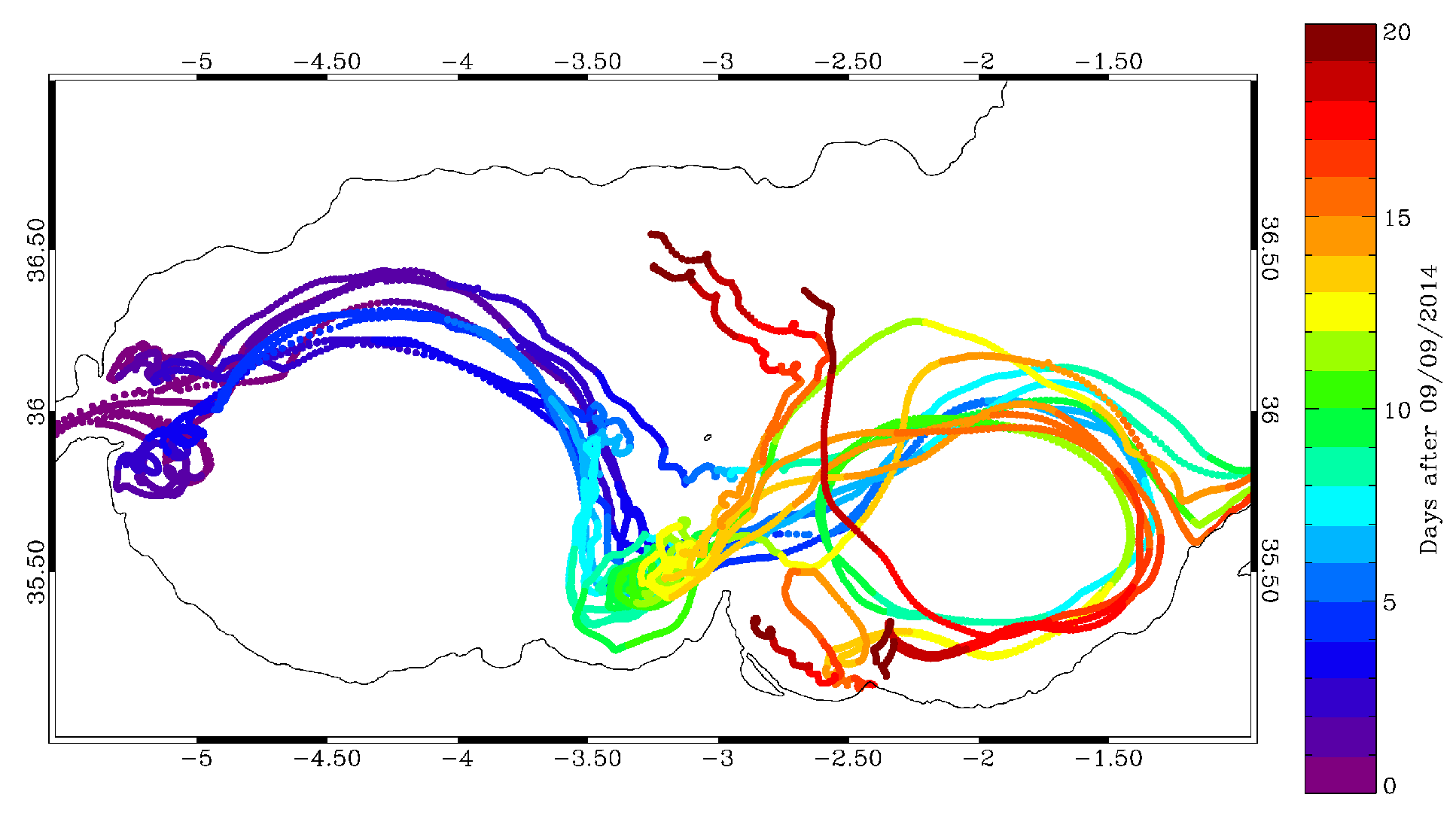
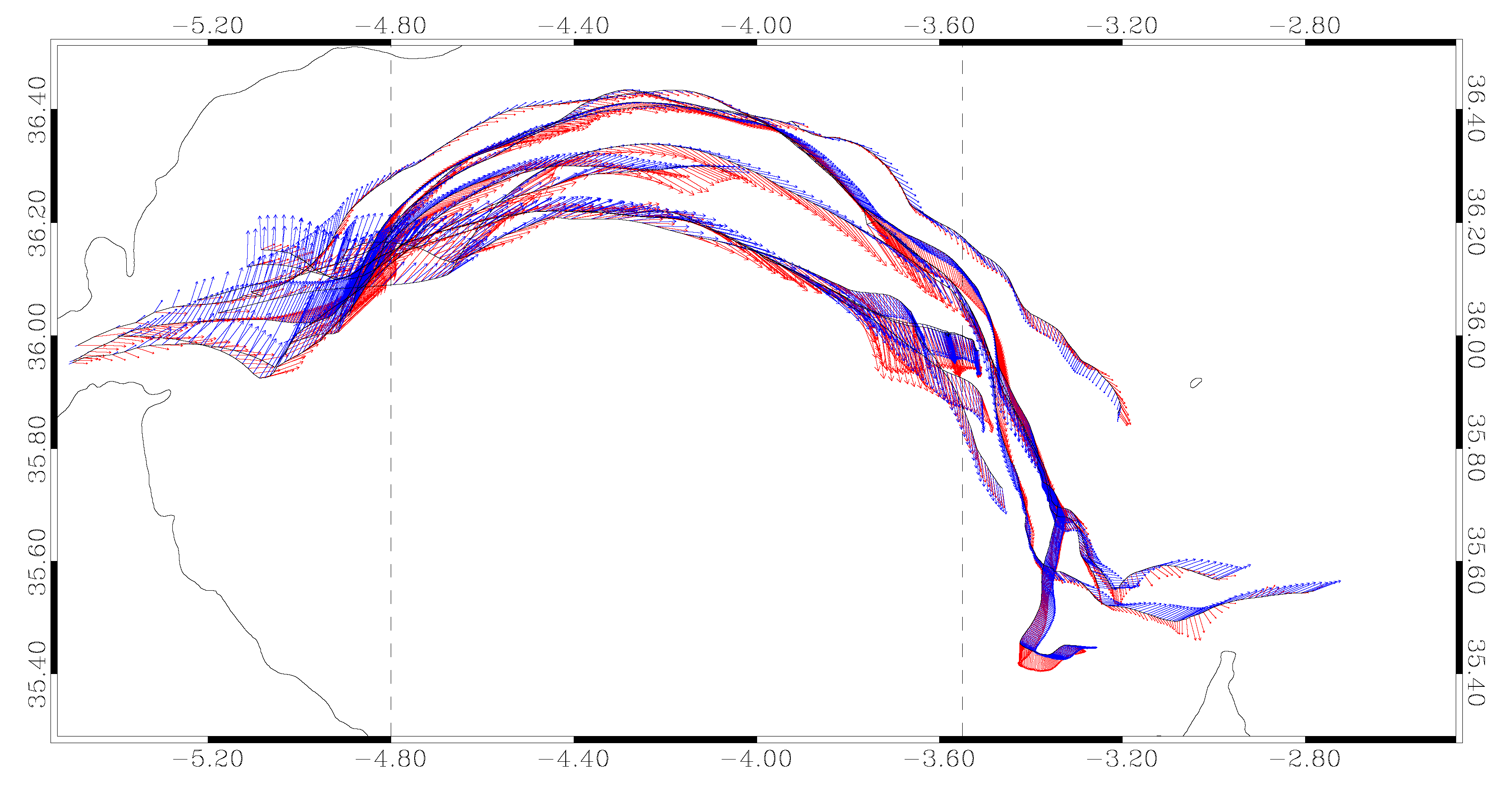
On the frame of the MEDESS-4MS project (EU MED Program), an intensive Lagrangian experiment was organized in the Strait of Gibraltar to validate and test the operational systems running in this area [16]. The experiment consisted od a quasi-synoptic deployment network of surface drifters distributed along the Strait of Gibraltar (Figure 2). The experiment started on 9 September and lasted around three months from September to December 2014. The drifters used in the experiment were mostly of CODE type [30] dragged at 1.5 m from the surface and a few units of oil-spills tracking drifters not used in this study, all set up with a sampling rate of 30 min. The dataset is available at PANGAEA (Data Publisher for Earth and Environmental Science) repository and all the quality control procedures and first view of the trajectories were described by Sotillo et al. [17].

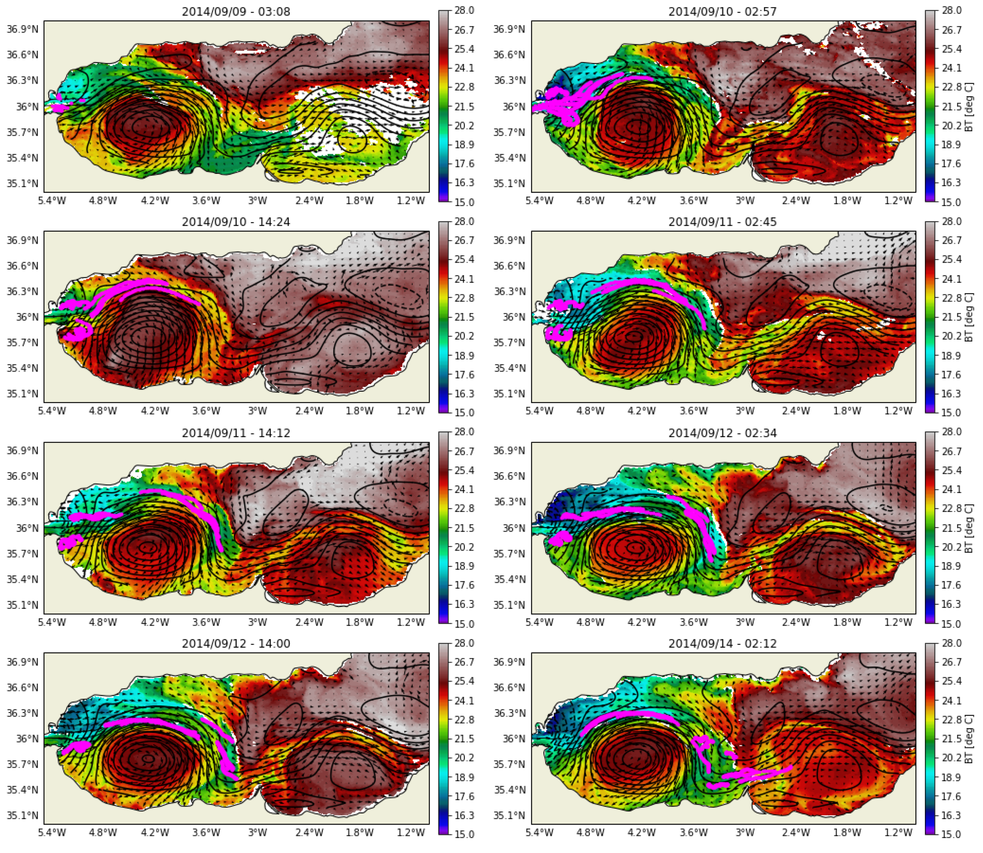
Geostrophic velocities used were derived from Near Real Time Absolute Dynamic Topography Maps (NRT-MADT) for the Mediterranean Sea generated by AVISO altimetry and distributed by the GlobCurrent project. Velocities were estimated from NRT-MADT using a nine-point stencil length, as described by Arbic et al. [31]. During the period, most drifters remained in the Alboran Sea (from 9 September to 29 September, Figure 2), but only 10 images with favorable cloud coverage were available. These images correspond to the AVHRR instrument from NOAA 19 platform for the period from 9 September at 03:08 GMT to 14 September at 02:12 GMT. Consequently, only the WAG could be simultaneously sampled by infrared instruments and drifters.

The used SSS corresponds to the Mediterranean and North Atlantic SMOS SSS maps V2.0 product from the Barcelona Expert Centre in Remote Sensing (BEC). These maps were derived from L1B Microwave Brightness Temperatures (MBT) products measured by SMOS and provided by ESA. Then, SMOS SSS daily L3 maps at $1/4^{\circ }\times 1/4^{\circ }$ resolution were produced by means of a successive corrections analysis applied over time periods of nine days using influence radii adapted to the Mediterranean Sea, see [32] and reference therein.

3. Reconstruction of Velocities from Thermal Images

3.1. Theoretical Background

Under the geostrophic approximation, surface velocities $\overrightarrow{v}(\overrightarrow{x})$ are non-divergent and are determined from a stream function $\psi (\overrightarrow{x})$

$$\overrightarrow{v}(\overrightarrow{x})={\overrightarrow{e}}_z\times \nabla \psi (\overrightarrow{x}),$$

(1)

which is proportional to sea surface height ($\eta (\overrightarrow{x})$, SSH), i.e.

$$\psi (\overrightarrow{x})=\frac{g}{f_0}\eta (\overrightarrow{x}).$$

(2)

Here, ${\overrightarrow{e}}_z$ is the vertical unit vector, $\overrightarrow{x}=(x,y)$, $f_0$ is the local Coriolis parameter, and g is the gravity constant.

When there is a strong correlation between sea surface buoyancy ($b_s(\overrightarrow{x})$, SSB) and potential vorticity (PV), it is possible to invert the quasi-geostrophic PV equations and derive the stream-function from SSB. For a semi-infinite ocean with constant stratification $N(z)=n_0{f}_0$, the stream function at any depth z is given by

$$\widehat{\psi }(\overrightarrow{k},z)=\frac{1}{n_e{f}_{0}k}{\widehat{b}}_s(\overrightarrow{k})exp(n_{0}kz),$$

(3)

where $\widehat{}$ stands for the Fourier transform, $n_e$ is an effective Prandtl ratio that takes into account the stratification and the interior PV, $\overrightarrow{k}=(k_x,k_y)$ is the wavevector, and $k=\parallel \overrightarrow{k}\parallel$ [22]. This is the so-called effective surface wuasi-geostrophic (eSQG) model.

Temperature and salinity are related to buoyancy through

$$b(\overrightarrow{x})=-\frac{g}{{\rho }_0}\left[\alpha (T(\overrightarrow{x})-T_0)+\beta (S(\overrightarrow{x})-S_0)\right],$$

(4)

where $\alpha <0$ is the thermal expansion coefficient, $-\beta >0$ is the haline contraction coefficient, and $T_0$ and $S_0$ are reference temperature and salinity, respectively. Then, assuming that temperature and salinity anomalies are related, Equation (4) can be approximated as

$$b(\overrightarrow{x})\approx -\frac{g}{{\rho }_0}\left[{\alpha }^{\prime }(T(\overrightarrow{x})-T_0)\right],$$

(5)

with ${\alpha }^{\prime }$ being an effective thermal expansion coefficient that takes into account the partial compensation between salinity and temperature [28]. Introducing this approximation to Equation (3), it is possible to derive surface currents from satellite observations of sea surface temperatures ($T_s(\overrightarrow{x})$, SST) [28]:

$$\widehat{\psi }(\overrightarrow{k},z)=-\frac{{\alpha }^{\prime }}{{\rho }_0{n}_e{f}_{0}k}{\widehat{T}}_s(\overrightarrow{k})exp(n_{0}kz).$$

(6)

Notice that this approach requires settin up the energy level of these velocities because of the presence of a free parameter ${\alpha }^{\prime }{n}_e^{-1}$ to take into account both interior PV and the partial compensation of salinity and temperature [28]. Interestingly, Equation (3) can also be used to derive buoyancy from SSH [28]

$$\widehat{b}(\overrightarrow{k},z)=n_{e}gk\widehat{\eta }(\overrightarrow{k})exp(n_{0}kz).$$

(7)

Equations (2), (6), and (7) relate key dynamical fields with satellite observations of SST and SSH.

3.2. Implementation

The diagnosis of surface currents from thermal images is straightforward using the SQG approach, if spatial resolutions below 5–10 km are not necessary. Following Isern-Fontanet and Hascoët [33], the surface stream function ($z=0$) is computed by applying Equation (6) to channel 4 brightness temperatures (BT) instead of SST due to their lower levels of noise. Before this, data gaps in BT images are filled using the approach of Isern-Fontanet et al. [28] and they are interpolated onto a doubly periodic regular grid. Then, geostrophic velocities are obtained using centered finite-differences and the free parameter ${\alpha }^{\prime }{n}_e^{-1}$ in Equation (6) is fixed imposing that the resulting velocity field has the same energy level as the velocity field derived from altimetry [28], i.e.,

$$\langle E_T\rangle \equiv \langle E_{\eta }\rangle ,$$

(8)

where $E_T(\overrightarrow{x})$ is the kinetic energy of the velocity field derived from thermal images, $E_{\eta }(\overrightarrow{x})$ is the kinetic energy of the velocity field derived from altimetry, and $\langle ·\rangle$ stands for the spatial average. Notice, however, that the velocity field derived from thermal images has a much higher spatial resolution than the field derived from altimetry. Therefore, $E_T(\overrightarrow{x})$ is first low-pass filtered with a cut-off wavelength of 60 km in order to determine the constant ${\alpha }^{\prime }{n}_e^{-1}$. It is worth mentioning that it is not necessary to have simultaneous observations of BT and SSH to calibrate the velocity field. Moreover, it is possible to use any other independent measurement of the velocities such as those obtained from HF radars, current-meters, or drifting buoys.

Figure 3 shows two examples of the SST representative of the period under study. These images unveil the presence of at least three different water masses: the warm waters associated to the WAG and EAG, a very warm water filling the northeast part of the Alboran Sea as well as the nearby Algerian basin, and a tongue of cold water newly entered from the Strait of Gibraltar that separates the previous ones. For this period, the EAG was smaller than the average situation and the front separating fresher waters from the saltier Mediterranean ones, usually located in the line Almeria–Oran, was displaced allowing Mediterranean waters to penetrate the Alboran basin, see [8] and references therein. The velocity field derived from thermal images correctly reproduce the currents associated to the WAG and partially the currents associated to the EAG. However, it also shows an intense current flowing from the southeast in the middle of the basin, i.e., along the limits of warm waters filling in the northeast of the image, which is not coherent with drifter trajectories (compare Figure 2 and Figure 3). These waters are, very likely, saline enough to dominate density and make this water mass denser than the waters of the Alboran vortices, rather than lighter as it would be expected from observed temperatures alone. Several arguments support this. First, previous in situ measurements showed that resident Mediterranean waters are saltier than the waters that form the Alboran vortices with typical salinities $S>38$ psu, e.g., [34]. Second, SSS maps derived from SMOS show the penetration of salty waters into the Alboran basing from the east (Figure 4). Third, buoyancy derived from altimetric maps using Equation (7) shows that this water mass, which is represented by the lined area in Figure 4, has less buoyancy and, consequently, it has to be more saline. Consequently, velocities have the opposite sign compared to velocities observed from drifters.

3.3. Phase Correction

The first approach to compute surface currents is to assume that temperature is a good proxy of density and, thus, the approach given by Equation (5) is valid. While this is a reasonable approach for the Alboran vortices and surrounding waters [29], results (Section 3.2, Figure 3) show that this is not valid for the warmer waters of the northeast. Consequently, the direct application of the eSQG model to these images produces velocities in the wrong sense in some parts of the image during this period of the year. Moreover, SSS from SMOS is not yet able to provide the necessary spatial resolution to correct full resolution infrared SST data, is not available in real time, and still slightly underestimates the dynamical range of SSS, see [26], for a more detailed discussion.

High resolution SST can still be used to derived currents if the dynamics in the area under study is dominated by the presence of water masses with distinctive salinity. Indeed, suppose there are M water masses with constant salinities $S_m$, where $m=1,\cdots ,M$. Then, Equation (4) becomes

$$b(\overrightarrow{x})=-\frac{g}{{\rho }_0}\left[\alpha (T(\overrightarrow{x})-T_0)+\beta \sum _{m=1}^M(S_m-S_0){\theta }_m(\overrightarrow{x})\right],$$

(9)

where ${\theta }_m(\overrightarrow{x})$ is a function such that

$${\theta }_m(\overrightarrow{x})=\left\{\begin{array}{cc}0\hfill & \mathrm{if}S(\overrightarrow{x})\ne S_m\hfill \\ 1\hfill & \mathrm{if}S(\overrightarrow{x})=S_m\hfill \end{array}\right.$$

(10)

with the additional property that

$$\sum _{m=1}^N{\theta }_m(\overrightarrow{x})=1.$$

(11)

This function segments the domain into non-overlapping areas with different constant salinities. Notice that these functions are also a function of time. If, as in the Alboran Sea, only two water masses are present, the above buoyancy can be written as

$$b(\overrightarrow{x})=-\frac{g}{{\rho }_0}\left[\alpha (T(\overrightarrow{x})-T_0)+\beta \Delta S(1-2{\theta }_{med}(\overrightarrow{x}))\right],$$

(12)

where the salinity of Atlantic waters is $S_{atl}=S_0-\Delta S$, the salinity of the Mediterranean waters is $S_{med}=S_0+\Delta S$, and ${\theta }_{med}(\overrightarrow{x})$ gives the extension of Mediterranean waters. The major practical difficulty is to determine the extension of Mediterranean waters, i.e to determine the function ${\theta }_{med}(\overrightarrow{x})$. Here, we compute ${\theta }_{med}(\overrightarrow{x})$ by computing the temperature anomaly and extracting the different water masses as the connected areas with the same sign of temperature anomaly. This idea is implemented by decomposing thermal images applying the à trous wavelets algorithm with B${}_3$-splines [33] and then removing the largest and the shortest scales. Finally, the wide, warm, and saltier mass located in the northeast can be identified as the largest connected area with positive temperature anomaly (lined area in Figure 4). Once the resident Mediterranean water mass has been identified, the effect of salinity can be corrected. To prove the concept and avoid numerical issues associated with the sharp transition of SSS, Equation (12) is further simplified to

$$b(\overrightarrow{x})\approx -\frac{g}{{\rho }_0}\left[{\alpha }^{\prime }(T(\overrightarrow{x})-T_0)(1-2{\theta }_{med}(\overrightarrow{x}))\right].$$

(13)

This approach implies that gradients of temperature and salinity tend to be aligned but with a change of sign in the different parts of the area under study (see Figure 2 in Isern-Fontanet et al. [24] and discussions in Isern-Fontanet et al. [24], Isern-Fontanet et al. [26]).

The application of Equation (6) to the corrected temperature anomalies given by Equation (13) provides more realistic results (Figure 5). Indeed, Atlantic waters now flow from west to east, as seen in previous studies [35] and in agreement with the trajectories of the drifters released during the MEDESS-GIB experiment (Figure 2). It is important to take into account that the transfer function between the stream function and temperature (or buoyancy) scales as ∼$k^{-1}$, which implies certain dominance of larger scales over smaller scales. This has as a consequence that the incorrect determination of the buoyancy sign for the Mediterranean waters can have a non-local impact. Therefore, ocean velocities around the WAG are wrongly diagnosed if this is not taken into account. Finally, its worth mentioning that the use of this crude approach (Equation (13)) instead of the approximation given by Equation (12) may affect the sign of the small scales in the Mediterranean waters. Nevertheless, we could not investigate this limitation due to the lack of data.

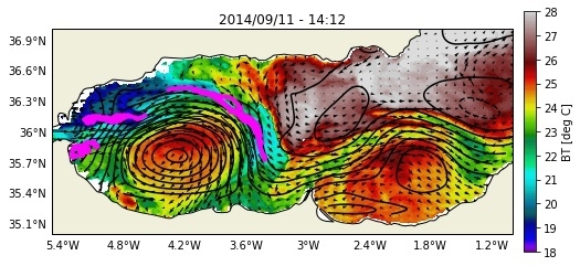
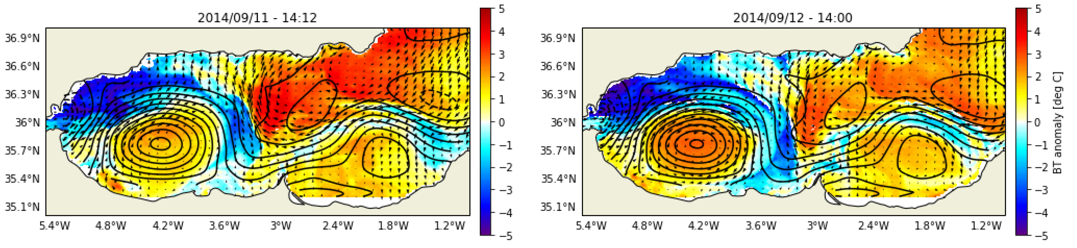
4. Comparison between Velocity Estimations

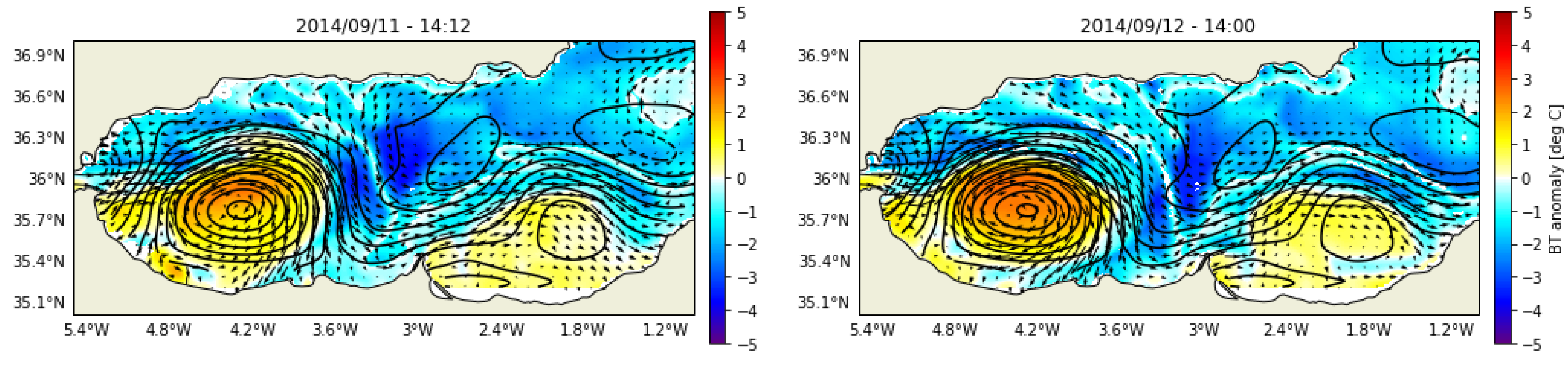
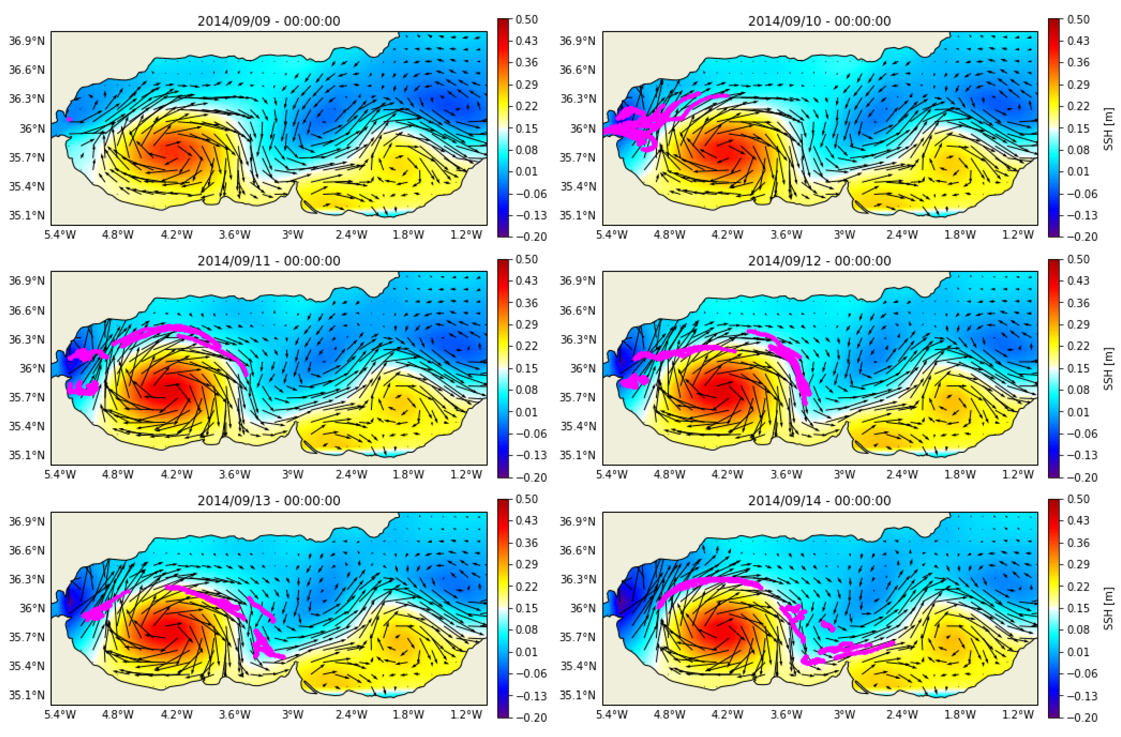
The eSQG model, together with the phase correction approach described in Section 3.3, were used to derive velocities from all the available thermal images (Figure 6 shows six of them). The resulting fields exhibit more temporal variability of the WAG than the velocity derived from SSH (Figure 6 and Figure 7). Indeed, thermal images shows that the WAG changes its shape significantly at temporal scales of the order of 12 h, but this variability is not observed in altimetric maps, which show an almost stationary vortex. A second major difference in the western part of the basin is the circulation east of the Strait of Gibraltar, the area between the strait and the vortex approximately limited by the meridian located at 4.8${}^{\circ }$W. There, altimetric maps show a northwards current while thermal images generate an eastwards current, indicating entrance of Atlantic waters into the Mediterranean Sea. The comparison between velocities derived from temperature and from sea level also show differences in the time evolution of the EAG. While the first shows an evolving vortex, altimetry shows an almost stationary bipolar structure. 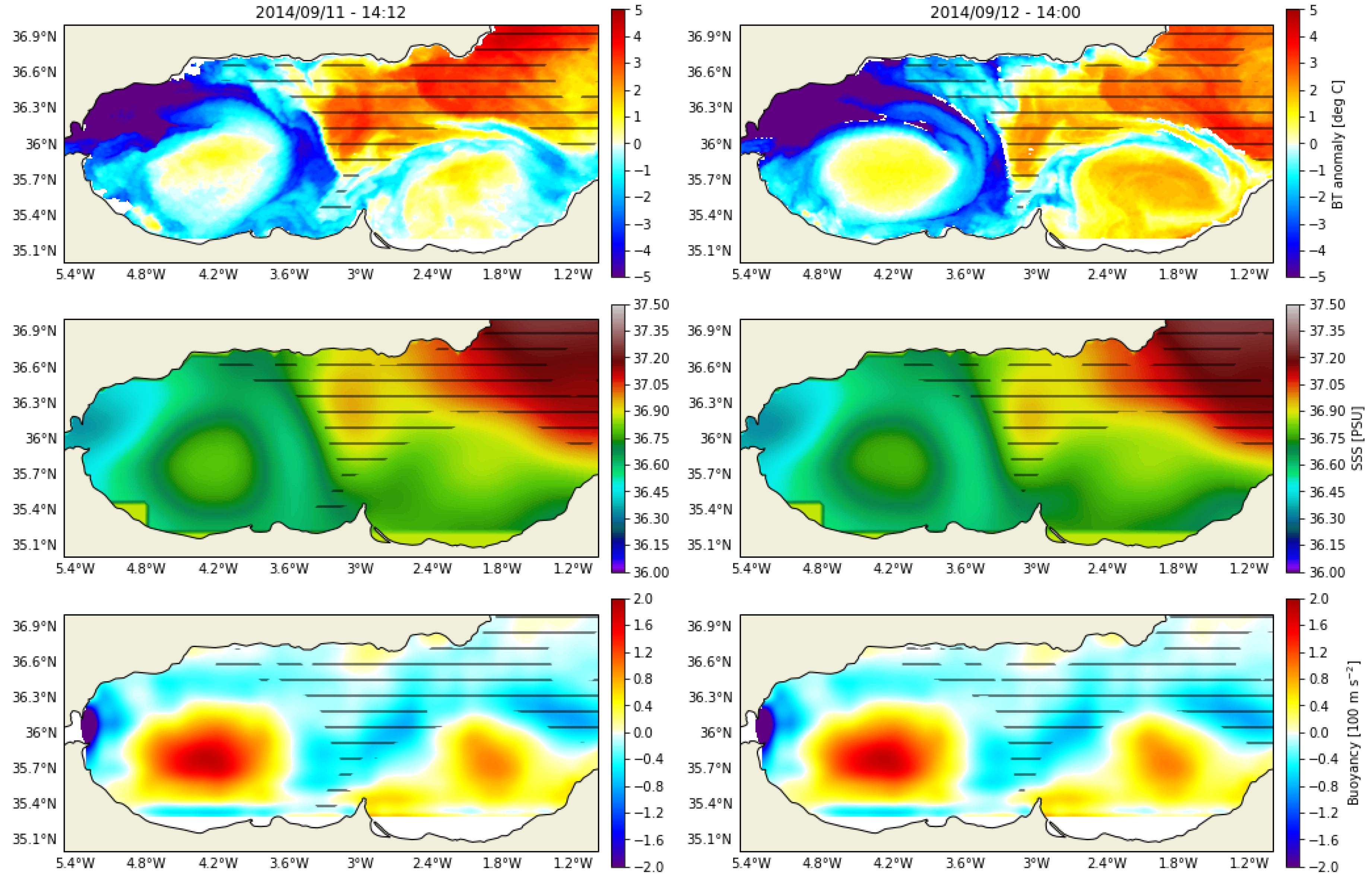The differences between altimetric and thermal images are also evident comparing BT and buoyancy derived from SSH (Figure 4). It is worth mentioning that, contrary to SST, buoyancy derived from SSH tends to be more representative of the patterns below the mixed layer rather than the ocean surface [28] and, consequently, fields may not be fully comparable. Nevertheless, the temporal evolution of this vortex and its characteristics points to sampling limitations of the altimetric measurements rather than the difference between density anomalies in the Mixed Layer and below it. Finally, both fields seem to capture the separation of the west–east flow from the WAG located around longitude 3.55${}^{\circ }$W. The exception is for the AVHRR image of 10 September at 14:24, which shows currents that do not agree with other satellite images or altimetric maps. The reason for this disagreement relies on the failure of the phase correction approach for this particular image. Indeed, the separation between the EAG and the large extension of warm waters is not good enough to correct for their contribution to the flow on this side of the basin.

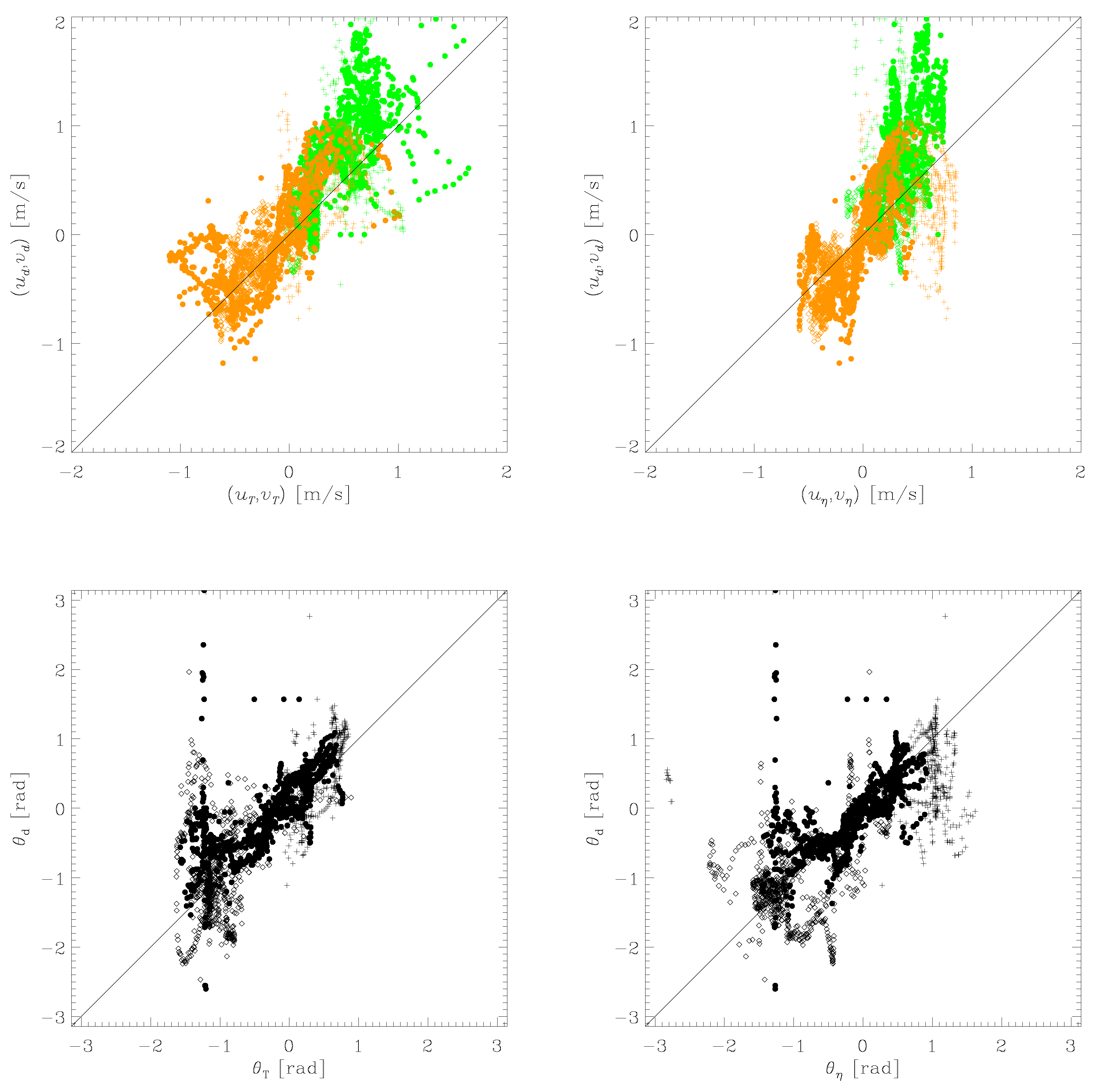
The velocity fields derived from altimetry and thermal images were compared to the in situ measurements provided by the drifters of the MEDESS-GIB experiment. A first comparison comes from the juxtaposition of trajectories with the instantaneous velocity fields (Figure 6 and Figure 7), which shows a strong tendency of drifter trajectories to move tangent to the velocity fields. There are, however, some exceptions, particularly in the area east of the Strait of Gibraltar where some drifters have swirling trajectories that do not agree with any of the velocity fields derived from satellite measurements. Although the temporal length of available thermal images is not long enough to analyze the penetration of drifters in the EAG, it is long enough to see the detachment of drifters from the WAG and their path towards the east, which is in agreement with the velocities seen from satellites. Notice that, in this area, swirling trajectories are also present and in disagreement with both velocity fields.

The velocities derived from surface drifters were compared to surface velocities derived from satellite observations by interpolating the latter onto the position and time of drifters (see Figure 8). Since no correction for the presence of inertial oscillations was applied, only those drifter segments that did not show small loops were taken from the whole set of drifters depicted in Figure 2. The global comparison between velocity components suggests a slightly better agreement between the velocities derived from SST than those derived from SSH (Figure 9). This can be seen in the global correlations between reconstructed velocities and drifter velocities, which are $r_u=0.63$ and $r_v=0.74$ for the velocities derived from SST and $r_u=0.48$ and $r_v=0.66$ for the velocities derived from SSH. Since some ageostrophic corrections modify the speed but do not modify the direction of the geostrophic current, e.g., the cyclostrophic flow, it is interesting to compare velocity directions. Here, the correlation between the velocity directions diagnosed from satellite and those derived from drifter trajectories are quite similar: $r_{\theta }=0.74$ for SST and $r_{\theta }=0.71$ for SSH. Notice, however, that all correlations are well below 0.9. Another difference between the two types of velocities derived from satellite observations is their kinetic energy. Although velocities derived from SST are calibrated with altimetric data, the lack of small scale signals in altimetric maps implies that higher resolution velocities derived from SST have to be low-pass filtered for calibration (Equation (8)) but the resulting field has higher kinetic energies closer to the kinetic energy of surface drifters (Figure 9).

Figure 8 shows a relatively good agreement in the direction of currents, i.e., small angles between velocities and drifter trajectories, in the WAG for both the velocities derived from altimetry and velocities derived from thermal images. However, there is an important difference in the velocity angles observed in the velocities derived from SST with respect to drifter velocities for values around −1.5 rad (Figure 9). This discrepancy is mainly due to the velocities in the eastern edge of the WAG. Moreover, between the Strait of Gibraltar and the WAG, altimetric velocities have angles that can be up to 90${}^{\circ }$ with respect to the trajectories of drifters while, velocities derived from thermal images show significantly smaller angles. The above observations and the patterns seen in the velocity fields (Figure 6 and Figure 7) suggest that the agreement between satellite derived and in situ velocities may not be homogeneous and point to define three different areas: the area east of Gibraltar (the area between the Strait of Gibraltar and meridian located at 4.8${}^{\circ }$W), the WAG (between the meridians located at 4.8${}^{\circ }$W and 3.45${}^{\circ }$W), and the bifurcation area (east of the meridian located at 3.45${}^{\circ }$W), where part of the flow is trapped by the WAG and part of it flows eastwards towards the EAG (see Figure 8). These areas were used to better quantify the agreement between in situ and satellite velocities. Taylor diagrams confirm that the ability to reconstruct velocities is better for WAG than for any other area (Figure 10), although velocities derived from temperature have slightly higher correlations for the direction. In the area east of the bifurcation point, on the contrary, the performance is better for altimetry, although correlations are quite low for the orientation of the current. The opposite situation is found in the area east of Gibraltar, in which altimetry shows very poor performance. Interestingly, the meridional velocity is better reconstructed than the zonal velocity for both SSH- and SST-derived velocities.

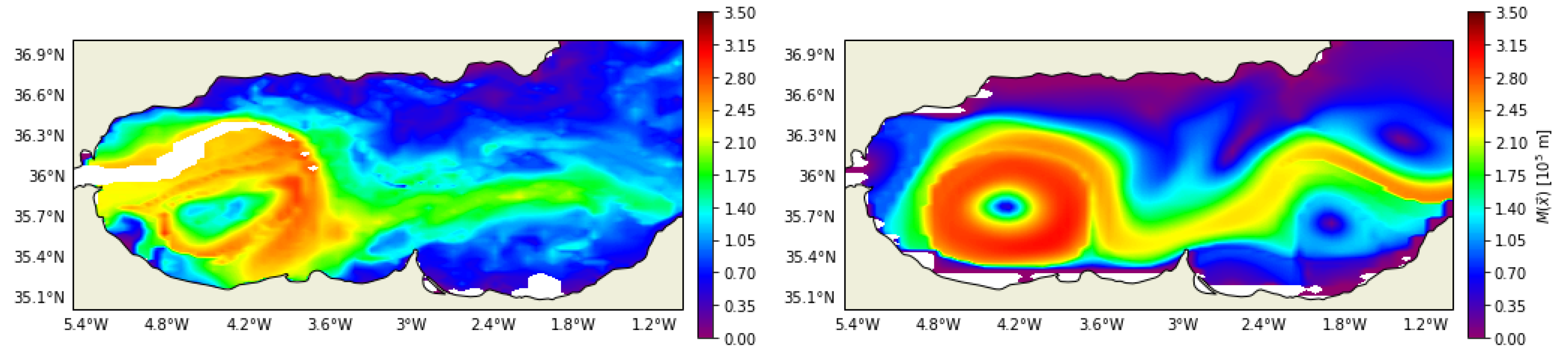
Finally, the topology of the two velocity fields derived from satellite observations was unveiled by using the methodology presented by Jiménez Madrid and Mancho [36], which has been already applied on altimeter datasets over the area of the Kuroshio Current [37]. The idea was to produce a two-dimensional field covering the region, which computes at each point the arc length of the trajectory passing for the point. More precisely, by using synthetic trajectories obtained integrating forwards and backwards for a determined amount of time and getting the distance travelled, the arc lengths of the trajectory are computed for the central instant of the time series to have the maximum possible time period to integrate, i.e., 2.5 days (see Appendix A for technical details). Figure 11 depicts the arc length plots for both velocity fields. One can see both velocity fields are able to capture the two-vortex patterns typical of the Alboran Sea but with significant differences. First, altimetric field is more stable, i.e., vortex cores are clearly delimited and the flow of Atlantic water is very well defined by large arc length values. This indicates, as already stated, that the temporal evolution of the altimetric field is slow. On the contrary, thermal field shows the effect of rapidly evolving WAG producing a vaguer structure but it is still possible to see the vortex core and its contour. It is worth mentioning that the detection of EAG is challenging due to the similar temperature it has with respect to the Mediterranean waters. It is only seen thanks to the flow of fresh waters that clearly separates both structures. Notice the strong differences between them. Second, the thermal field is able to capture the entrance of Atlantic waters while the altimetric field is not. Indeed, the shadowed area in Figure 11 is due to the particles that escape from the domain; consequently, it is not possible to track their evolution for the entire time period considered. It is worth remarking that, in the plot corresponding to the altimetric field, there are big regions of very low arc length values (purple color in the figure), showing the limitation of the altimetric fields when one approaches the coast in comparison to the velocities derived from SST.

5. Discussion

The circulation in the Alboran Sea is usually dominated by the presence of two large vortices that dominate the upper 100–300 m of the ocean [34,38]. These conditions are favorable to the exploitation of the eSQG approximation to retrieve surface current, as shown by LaCasce and Mahadevan [29] and confirmed by the results shown in Section 4. This opens the door to use SST to retrieve surface currents in this area, which allows resolving both the high frequency evolution of these vortices and the smaller scales structures that surround them [12]. On the contrary, Altimeters have spatial and temporal sampling limitations. Alboran vortices, however, are large enough to be properly sampled by altimeters. Consequently, both velocities derived from infrared radiometers and velocities derived from radar altimeters show similar capabilities when compared with the trajectories of drifting buoys. Nevertheless, there are some relevant exceptions: the area east of Gibraltar. This area is not properly sampled by altimeters and, therefore, velocities diagnosed in this zone are significantly different from those observed by drifting buoys. On the contrary, velocities derived from thermal images give velocities with directions relatively close to the observed by drifters ($\langle |{\theta }_{\eta }-{\theta }_d|\rangle ={40.2}^{\circ }$ while $\langle |{\theta }_T-{\theta }_d|\rangle ={19.3}^{\circ }$). The comparison between drifters and the geostrophic velocities derived from SST or SSH, however, has an important drawback: drifter trajectories have ageostrophic contributions not taken into account in the derivation of surface currents from SST nor SSH. In particular, drifters are affected by wind [39] and inertial oscillations as well as ageostrophic contributions such as the cyclostrophic flow associated to the curvature of the Alboran vortex. Furthermore, drifter speed in the area east of Gibraltar showed some temporal behavior that suggest a relevant contribution from tides.

Although thermal images and altimeter maps have similar performances when the flow is dominated by structures large enough to be sampled by altimeters, both approaches have different latencies, with that of currents derived from SST being of the order of few hours (typically less than 4 h) (This is the time passed between satellite measurement and the delivery of surface currents derived from them. Notice that the time needed to estimate currents from SST is of the order of the time needed to compute the FFT). Of course, velocities have to be calibrated and independent measurements such as the ones provided by altimeters are necessary; however, when only the energy level has to be fixed, simultaneous data are not needed. On the contrary, it requires some time to get accurate altimetric measurements and near-real time maps can only use past data, which further limits the capability to resolve two-dimensional structures if not enough altimeters are available [18]. Thermal images have, however, two main limitations. First, they can only be used under cloud-free situations, which restricts their applicability (particularly for those methods requiring consecutive cloud free images such optical flow and MCC). It is worth mentioning that the Mediterranean Sea is a quite favorable situation, with a relatively large fraction of cloud-free images (∼$40\%$). For moving clouds, gaps can be filled combining several images. One possible approach would be to compute vorticity from SST for several images, calibrate them, combine vorticities for a short enough period of time, and, finally, recompute the stream function inverting the vorticity.

A second limitation, as discussed above, is the need to correct for the impact of SSS. Presently, SSS measurements are not available in real time, although important advances have been done and it is already possible to detect the signature of the Atlantic waters in the Algerian basin [26] and the key patterns in the Alboran Sea with low resolutions. This implies that other approaches are needed. Here, we explored a simple method that consists of detecting Mediterranean waters from thermal images and modifing y buoyancy to take into account the effect of salinity. Although this approach is very crude, it shows that it is able to correct the role of salinity and provide results similar to those provided by altimeters. This raises a question: To what extent can the approach here proposed be used in other areas of the ocean? As shown in Section 3.3, there are two necessary conditions: the existence of water masses with salinities homogeneous enough to be considered constant and a way to identify such water masses from existing satellite observations. Multiple strategies are possible to identify water masses. In areas dominated by the presence of vortices of distinctive salinity, e.g., the Algerian basin [26], vortex identification techniques can be used [40,41]. In areas where SST univocally identifies water masses, temperature can be used to identify the extension of water masses. In other cases, image processing techniques combined with oceanographic knowledge can be applied to satellite observations of temperature or chlorophyll to segment the image. Future improvements could include the use of new SSS products (if they are available in real time), climatological SSS, or the exploitation of the buoyancy derived from altimetry to give a better estimation of density anomalies. However, these approaches require the implementation of accurate numerical methods that are beyond the scope of this study.

6. Conclusions

This study provides further evidence that the SQG approach is able to reconstruct velocities in the Alboran Sea. Moreover, the results show that altimetric measurements do s not capture the temporal evolution of the WAG while infrared measurements do, which can be used to derive surface velocities in this area, although the role of salinity can limit this approach. Nevertheless, the strong relationship between salinity and temperature allows identifying the water masses and correct for the contribution of salinity using image processing techniques. Once corrected, the SQG approach can retrieve ocean currents slightly better to that of near-real-time currents in general but much better in areas badly sampled by altimeters such as the area east of the Strait of Gibraltar. Although this area is far from the geostrophic equilibrium, the above results show that the good sampling capabilities of infrared radiometers allows at least retrieving the direction of ocean currents in this area. These results can be extended to other areas of the ocean, provided that water masses with relatively homogeneous salinity can be identified from remote sensing measurements.

References

1. Mercado, J.M.; Cortés, D.; García, A.; Ramírez, T. Seasonal and inter-annual changes in the planktonic communities of the northwest Alboran Sea (Mediterranean Sea). Prog. Oceanogr. 2007, 74, 273–293. [Google Scholar] [CrossRef]
2. Huertas, I.; Ríos, A.; García-Lafuente, J.; Navarro, G.; Makaoui, A.; Sánchez-Román, A.; Rodriguez-Galvez, S.; Orbi, A.; Ruíz, J.; Pérez, F.F. Atlantic forcing of the Mediterranean oligotrophy. Glob. Biogeochem. Cycle 2012, 26, GB2022. [Google Scholar] [CrossRef] [Green Version]
3. Lo Iacono, C.; Gràcia, E.; Ranero, C.; Emelianov, M.; Huvenne, V.; Bartolomé, R.; Booth-Rea, G.; Prades, J. The West Melilla cold water coral mounds, Eastern Alboran Sea: Morphological characterization and environmental context. Deep Sea Res. Part II Top. Stud. Oceanogr. 2014, 99, 316–326. [Google Scholar] [CrossRef]
4. REMPEC. Study of Maritime Traffic Flows in the Mediterranean Sea. Regional Marine Pollution Emergency Response Centre for the Mediterranean Sea (REMPEC); Technical Report; Lloyd’s Marine Intelligence Unit: Valletta, Malta, 2008. [Google Scholar]
5. Lacombe, H. Contribution à l’étude du détroit de Gibraltar. I. Etude dynamique. Cahiers Ocdanographiques 1961, XllI, 73–107. [Google Scholar]
6. Stommel, H.; Bryden, H.; Mangelsdorf, P. Does some of the Mediterranean outflow come from great depth? Pure Appl. Geophys. 1973, 105, 879–889. [Google Scholar] [CrossRef]
7. Gascard, J.; Richez, C. Water masses and circulation in the western Alborán Sea and in the Straits of Gibraltar. Prog. Oceanogr. 1985, 15, 157–216. [Google Scholar] [CrossRef]
8. Sánchez-Garrido, J.; García Lafuente, J.; Álvarez Fanjul, E.; García Sotillo, M.; de los Santos, F. What does cause the collapse of the Western Alboran Gyre? Results of an operational ocean model. Prog. Oceanogr. 2013, 116, 142–153. [Google Scholar] [CrossRef]
9. Bryden, H.; Kinder, T. Steady two-layer exchange through the Strait of Gibraltar. Deep Sea Res. Part A 1991, 38, S445–S463. [Google Scholar] [CrossRef]
10. Naranjo, C.; Garcia-Lafuente, J.; Sannino, G.; Sanchez-Garrido, J. How much do tides affect the circulation of the Mediterranean Sea? From local processes in the Strait of Gibraltar to basin-scale effects. Prog. Oceanogr. 2014, 127, 108–116. [Google Scholar] [CrossRef]
11. García-Lafuente, J.; Naranjo, C.; Sammartino, S.; Sánchez-Garrido, J.; Delgado, J. The Mediterranean Outflow in the Strait of Gibraltar and its connection with upstream conditions in the Alborán Sea. Ocean Sci. Discuss 2016. in review. [Google Scholar] [CrossRef]
12. Tintoré, J.; Gomis, D.; Alonso, S.; Parrilla, G. Mesoscale Dynamics and Vertical Motion in the Alborán Sea. J. Phys. Oceanogr. 1991, 21, 811–823. [Google Scholar] [CrossRef] [Green Version]
13. Viúdez, A.; Haney, R.L.; Vazquez-Cuervo, J. The deflection and division of an oceanic baroclinic jet by a coastal boundary: A case study in the Alboran sea. J. Phys. Oceanogr. 1998, 28, 289–308. [Google Scholar] [CrossRef]
14. Renault, L.; Oguz, T.; Pascual, A.; Vizoso, G.; Tintore, J. Surface circulation in the Alborán Sea (western Mediterranean) inferred from remotely sensed data. J. Geophys. Res. Ocean. 2012, 117, C08009. [Google Scholar] [CrossRef] [Green Version]
15. Peliz, A.; Boutov, D.; Teles-Machado, A. The Alboran Sea mesoscale in a long term high resolution simulation: Statistical analysis. Ocean Model. 2013, 72, 32–52. [Google Scholar] [CrossRef]
16. Sotillo, M.G.; Garcia-Ladona, E.; Orfila, A.; Rodríguez-Rubio, P.; Maraver, J.C.; Conti, D.; Padorno, E.; Jiménez, J.A.; Capó, E.; Pérez, F.; et al. The MEDESS-GIB database: Tracking the Atlantic water inflow. Earth Syst. Sci. Data 2016, 8, 141–149. [Google Scholar] [CrossRef] [Green Version]
17. Sotillo, M.; Amo-Baladrón, A.; Padorno, E.; Garcia-Ladona, E.; Orfila, A.; Rodríguez-Rubio, P.; Conti, D.; Madrid, J.J.; de los Santos, F.; Fanjul, E.A. How is the surface Atlantic water inflow through the Gibraltar Strait forecasted? A lagrangian validation of operational oceanographic services in the Alboran Sea and the Western Mediterranean. Deep Sea Res. Part II Top. Stud. Oceanogr. 2016, 133, 100–117. [Google Scholar] [CrossRef] [Green Version]
18. Pascual, A.; Faugere, Y.; Larnicol, G.; Le Traon, P. Improved description of the ocean mesoscale variability by combining four satellite altimeters. Geophys. Res. Lett. 2006, 33, L02611. [Google Scholar] [CrossRef] [Green Version]
19. Isern-Fontanet, J.; Ballabrera-Poy, J.; Turiel, A.; García-Ladona, E. Remote sensing of ocean surface currents: A review of what is being observed and what is being assimilated. Nonlinear Process. Geophys. 2017, 24, 613–643. [Google Scholar] [CrossRef] [Green Version]
20. Held, I.; Pierrehumbert, R.; Garner, S.; Swanson, K. Surface quasi-geostrophic dynamics. J. Fluid Mech. 1995, 282, 1–20. [Google Scholar] [CrossRef]
21. Lapeyre, G. Surface Quasi-Geostrophy. Fluids 2017, 2, 7. [Google Scholar] [CrossRef]
22. Lapeyre, G.; Klein, P. Dynamics of the Upper Oceanic Layers in Terms of Surface Quasigeostrophy Theory. J. Phys. Oceanogr. 2006, 36, 165–176. [Google Scholar] [CrossRef]
23. Isern-Fontanet, J.; Chapron, B.; Klein, P.; Lapeyre, G. Potential use of microwave SST for the estimation of surface ocean currents. Geophys. Res. Lett. 2006, 33, L24608. [Google Scholar] [CrossRef] [Green Version]
24. Isern-Fontanet, J.; Shinde, M.; González-Haro, C. On the transfer function between surface fields and the geostrophic stream function in the Mediterranean sea. J. Phys. Ocean 2014, 44, 1406–1423. [Google Scholar] [CrossRef]
25. González-Haro, C.; Isern-Fontanet, J. Reconstruction of global surface currents from passive microwave radiometers. J. Geophys. Res. 2014, 119. [Google Scholar] [CrossRef]
26. Isern-Fontanet, J.; Olmedo, E.; Turiel, A.; Ballabrera-Poy, J.; García-Ladonaía-Ladona, E. Retrieval of eddy dynamics from SMOS sea surface salinity measurements in the Algerian Basin (Mediterranean Sea). Geophys. Res. Lett. 2016, 43. [Google Scholar] [CrossRef] [Green Version]
27. Ponte, A.; Klein, P. Reconstruction of the upper ocean 3D dynamics from high-resolution sea surface height. Ocean Dyn. 2013, 63, 777–791. [Google Scholar] [CrossRef]
28. Isern-Fontanet, J.; Lapeyre, G.; Klein, P.; Chapron, B.; Hetcht, M. Three-dimensional reconstruction of oceanic mesoscale currents from surface information. J. Geophys. Res. 2008, C09005. [Google Scholar] [CrossRef] [Green Version]
29. LaCasce, J.; Mahadevan, A. Estimating subsurface horizontal and vertical velocities from sea surface temperature. J. Mar. Res. 2006, 64, 695–721. [Google Scholar] [CrossRef] [Green Version]
30. Davis, R.E. Drifter observations of coastal surface currents during CODE: The statistical and dynamical views. J. Geophys. Res. Ocean. 1985, 90, 4756–4772. [Google Scholar] [CrossRef]
31. Arbic, B.; Scott, R.; Chelton, D.; Richman, J.; Shriver, J. Effects of stencil width on surface ocean geostrophic velocity and vorticity estimation from gridded satellite altimeter data. J. Geophys. Res. Ocean. 2012, 117, C03029. [Google Scholar] [CrossRef] [Green Version]
32. Olmedo, E.; Taupier-Letage, I.; Turiel, A.; Alvera-Azcárate, A. Improving SMOS Sea Surface Salinity in the Western Mediterranean Sea through Multivariate and Multifractal Analysis. Remote Sens. 2018, 10. [Google Scholar] [CrossRef] [Green Version]
33. Isern-Fontanet, J.; Hascoët, E. Diagnosis of high resolution upper ocean dynamics from noisy sea surface temperature. J. Geopys. Res. 2014, 118, 1–12. [Google Scholar] [CrossRef] [Green Version]
34. Viúdez, A.; Tintoré, J.; Haney, R.L. Circulation in the Alboran sea as determined by quasi-synoptic hydrographic observations. Part I: Three-dimensional structures of two anticyclonic gyres. J. Phys. Oceanogr. 1996, 26, 684–705. [Google Scholar] [CrossRef]
35. Millot, C. Circulation in the Western Mediterranean Sea. J. Mar. Syst. 1999, 20, 423–442. [Google Scholar] [CrossRef] [Green Version]
36. Jiménez Madrid, J.A.; Mancho, A.M. Distinguished trajectories in time dependent vector fields. Chaos: Interdiscip. J. Nonlinear Sci. 2009, 19, 013111. [Google Scholar] [CrossRef] [PubMed] [Green Version]
37. Mendoza, C.; Mancho, A.M. Review Article: “The Lagrangian description of aperiodic flows: A case study of the Kuroshio Current”. Nonlinear Process. Geophys. 2012, 19, 449–472. [Google Scholar] [CrossRef] [Green Version]
38. Tintore, J.; Violette, P.E.L.; Blade, I.; Cruzado, A. A Study of an Intense Density Front in the Eastern Alboran Sea: The Almeria–Oran Front. J. Phys. Oceanogr. 1988, 18, 1384–1397. [Google Scholar] [CrossRef]
39. Poulain, P.M.; Gerin, R.; Mauri, E.; Pennel, R. Wind Effects on Drogued and Undrogued Drifters in the Eastern Mediterranean. J. Atmos. Ocean. Technol. 2009, 26, 1144–1156. [Google Scholar] [CrossRef]
40. Isern-Fontanet, J.; García-Ladona, E.; Font, J. Identification of Marine eddies from Altimetry. J. Atmos. Ocean. Technol. 2003, 20, 772–778. [Google Scholar] [CrossRef]
41. Isern-Fontanet, J.; García-Ladona, E.; Font, J. The vortices of the Mediterranean sea: An altimetric perspective. J. Phys. Oceanogr. 2006, 36, 87–103. [Google Scholar] [CrossRef] [Green Version]
42. Mancho, A.M.; Small, D.; Wiggins, S. A comparison of methods for interpolating chaotic flows from discrete velocity data. Comput. Fluids 2006, 35, 416–428. [Google Scholar] [CrossRef]
Figure 1. Scheme of the surface circulation in the Alboran Sea showing the western and eastern Alboran gyres (WAG and EAG) as well as the jet of Atlantic waters (AJ), from Sánchez-Garrido et al. [8].
Remotesensing 12 00724 g001
Figure 2. Trajectories of surface drifters for the MEDGIB-GIB experiment. Color scale corresponds to time with respect to 9 September 2014.
Remotesensing 12 00724 g002
Figure 3. Brightness temperature anomaly derived from AVHRR’s channel 4 measurements corresponding to: 11 September at 14:12 GMT (left); and 12 September at 14:00 GMT (right). Arrows show the velocity field derived from the images.
Remotesensing 12 00724 g003
Figure 4. Brightness temperature anomaly derived from satellite measurements (top); sea surface salinity derived from SMOS (middle); and surface buoyancy derived from altimetric maps (bottom) corresponding to: 11 September at 14:12 GMT (left); and 12 September (right) at 14:00 GMT. Lined area identifies resident Mediterranean waters obtained using the method described in Section 3.3.
Remotesensing 12 00724 g004
Figure 5. Corrected brightness temperature anomaly corresponding to: 11 September at 14:12 GMT (left); and 12 September (right) at 14:00 GMT. Arrows show the velocity field derived from the images.
Remotesensing 12 00724 g005
Figure 6. Sequence of corrected brightness temperature with the associated geostrophic velocities. Magenta dots correspond to the position of drifters within the the period of ±0.5 days around the map date.
Remotesensing 12 00724 g006
Figure 7. Absolute dynamic topography and associated geostrophic velocities. Magenta dots correspond to the position of drifters within the the period of ±0.5 days around the map date.
Remotesensing 12 00724 g007
Figure 8. Drifter trajectories for the period under analysis and velocities derived from the IR radiometer (red) and the Radar Altimeter (blue) interpolated onto drifter position and time. The vertical line indicates the longitude used to separate the area east of Gibraltar from the WAG. Black lines correspond to the same trajectories shown in the upper panel.
Remotesensing 12 00724 g008
Figure 9. Scatter plot between the drifter velocities (ordinate) and the velocities derived from thermal images (abscissa, left) and altimetry (abscissa, right). Green corresponds to zonal velocity, orange to meridional velocity, and black to the velocity angle with respect to the east–west direction. Diamonds correspond to the area east of the Strait of Gibraltar, dots to the central part of the WAG, and crosses to the eastern area of the vortex (see Figure 8).
Remotesensing 12 00724 g009
Figure 10. Taylor diagram for zonal (orange) and meridional (green) velocity components and velocity direction (black) for the area east of Gibraltar (cross), WAG (circle) and stagnation point (diamond): (top) velocities derived from thermal images; and (bottom) velocities derived from altimetry. To facilitate the comparison, standard deviations were normalized by the standard deviations of drifters given in Table 1.
Remotesensing 12 00724 g010
Figure 11. Arc length of the trajectory for the central time of the period analyzed for the velocity fields derived from: thermal images (top); and altimetry (bottom). The white area west of the Strait of Gibraltar corresponds to the point at which particles escape through the Strait of Gibraltar when integrating backwards.
Remotesensing 12 00724 g011