Article

Characterizing Land Surface Phenology and Exotic Annual Grasses in Dryland Ecosystems Using Landsat and Sentinel-2 Data in Harmony

1
KBR, Contractor to the U.S. Geological Survey, Earth Resources Observation and Science Center, Sioux Falls, SD 57198, USA
2
U.S. Geological Survey, Earth Resources Observation and Science Center, Sioux Falls, SD 57198, USA
3
U.S. Geological Survey, National Land Imaging Program, Flagstaff, AZ 86001, USA
*
Author to whom correspondence should be addressed.
Submission received: 4 February 2020 / Revised: 20 February 2020 / Accepted: 20 February 2020 / Published: 22 February 2020
(This article belongs to the Special Issue Remote Sensing of Dryland Environment)

Abstract

:
Invasive annual grasses, such as cheatgrass (Bromus tectorum L.), have proliferated in dryland ecosystems of the western United States, promoting increased fire activity and reduced biodiversity that can be detrimental to socio-environmental systems. Monitoring exotic annual grass cover and dynamics over large areas requires the use of remote sensing that can support early detection and rapid response initiatives. However, few studies have leveraged remote sensing technologies and computing frameworks capable of providing rangeland managers with maps of exotic annual grass cover at relatively high spatiotemporal resolutions and near real-time latencies. Here, we developed a system for automated mapping of invasive annual grass (%) cover using in situ observations, harmonized Landsat and Sentinel-2 (HLS) data, maps of biophysical variables, and machine learning techniques. A robust and automated cloud, cloud shadow, water, and snow/ice masking procedure (mean overall accuracy >81%) was implemented using time-series outlier detection and data mining techniques prior to spatiotemporal interpolation of HLS data via regression tree models (r = 0.94; mean absolute error (MAE) = 0.02). Weekly, cloud-free normalized difference vegetation index (NDVI) image composites (2016–2018) were used to construct a suite of spectral and phenological metrics (e.g., start and end of season dates), consistent with information derived from Moderate Resolution Image Spectroradiometer (MODIS) data. These metrics were incorporated into a data mining framework that accurately (r = 0.83; MAE = 11) modeled and mapped exotic annual grass (%) cover throughout dryland ecosystems in the western United States at a native, 30-m spatial resolution. Our results show that inclusion of weekly HLS time-series data and derived indicators improves our ability to map exotic annual grass cover, as compared to distribution models that use MODIS products or monthly, seasonal, or annual HLS composites as primary inputs. This research fills a critical gap in our ability to effectively assess, manage, and monitor drylands by providing a framework that allows for an accurate and timely depiction of land surface phenology and exotic annual grass cover at spatial and temporal resolutions that are meaningful to local resource managers.

Graphical Abstract

1. Introduction

Increasing spread of invasive vegetation, such as cheatgrass (Bromus tectorum L.), can contribute to ecosystem degradation and increased disturbance frequency within dryland ecosystems that cover roughly 40% of the Earth’s land surface [1,2,3]. Several invasive annual grass species are present in the sagebrush biome of the western United States, but cheatgrass is the most ubiquitous, especially in the Great Basin, which includes most of Nevada and portions of Utah, Idaho, Wyoming, Oregon, and California [4]. Cheatgrass has a relatively long history in the area, prolific seed production characteristics [5,6], and an ability to outcompete most native vegetation after disturbances and for early growing season moisture [7]. Changing climate and disturbance regimes may drive exotic annual grasses into uninvaded areas [8,9,10] further diminishing ecosystem services [11]. Monitoring and mapping of exotic annual grass dynamics is therefore vital for land resource managers in the stewardship of dryland environments [12,13].
Emerging technologies and remote sensing sensors have spawned a deluge of information and tools that are useful for characterizing invasive plants and fractional components of dryland communities at local to regional scales [14,15,16]. Previous studies have used information collected by a suite of remote sensing platforms (e.g., Moderate Resolution Image Spectroradiometer (MODIS), Landsat, Advanced Very High Resolution Radiometer (AVHRR)) to quantify spatiotemporal patterns of invasive plant species [17], including cheatgrass cover and die-off [18,19,20,21], and associated drivers of invasion at local and regional scales [17,22,23]. Remote sensing of exotic annual grasses in dryland ecosystems of the western United States has largely relied on repeat, multispectral imagery and phenological difference techniques; where some exotic annual grasses are characterized by early spring green-up, senescence, and amplified inter-annual growth response to precipitation that is distinct from most native species [24,25,26]. Distribution models and maps of exotic annual grass cover support early detection and rapid response initiatives if data inputs have high spectral, spatial, and temporal resolution (or if proliferation is distinct, homogenous, or slow growing), but few studies have made use of technologies that provide accurate and spatially-detailed information at latencies requested by land resource managers.
The overarching goal of this research was to develop a fully automated and scalable system that leverages in situ observations, harmonized Landsat and Sentinel-2 (HLS) data and derived metrics (i.e., phenological and spectral indices), and data mining techniques for mapping exotic annual grass (%) cover (30-m spatial resolution) throughout dryland ecosystems in the western United States. We defined the following objectives to accomplish this goal, which provides guidance for the organization of the remainder of the manuscript: (1) Develop a robust, automated cloud, cloud shadow, water, and snow/ice masking approach for harmonized Landsat 8 and Sentinel-2 data using image differencing techniques in a semi-supervised classification framework; (2) train and validate regression tree models for accurate interpolation of HLS spectral data through space and time; (3) identify remote sensing and derived information (e.g., phenological and time-series metrics, topographical, and biophysical data) that are most useful for explaining the spatial patterns of exotic annual grass cover; and (4) construct regression tree models using in situ and remote sensing observations to develop spatially explicit estimates of exotic annual grass (%) cover and associated estimates of uncertainty. Our approach using harmonized Landsat and Sentinel-2 data facilitates expedited mapping of exotic annual grass cover across large regions at unparalleled spatial and temporal resolutions.

2. Material and Methods

2.1. Automated Cloud, Shadow, Snow/Ice, and Water Masking Procedure

The study area was divided into 33 production units (109.8 km × 109.8 km) based on the Sentinel-2 tiling system, spanning portions of Oregon, California, Idaho, and Nevada (Figure 1). Harmonized Landsat and Sentinel-2 (HLS) data scenes (v1.4) were pulled from the HLS data download site, filtered by acquisition week (i.e., weeks 4 to 44). Readers are referred to [27] for a detailed review of HLS imagery and preprocessing. In total, there were approximately 12,000 scenes that met our filtering criteria from 2016 to 2018.
We developed an automated masking procedure leveraging HLS imagery and decision tree classification models because of known issues with the standard (v1.4) HLS masking layers. Training examples needed for decision tree classifiers were harvested using quality assurance (QA) band information and spectral thresholding for each Landsat and Sentinel-2 scene. Pixels identified to be clouds/shadows/water/snow/ice in the QA bands and those with a Normalized Difference Wetness Index (NDWI) ≤0.05 were given a value of 0. Conversely, pixels with high-quality information and NDWI values >0.05 were give a value of 1 because qualitative analysis indicates this to be a reasonable threshold for improving shadow and water detection. Coincident spectral information (all available bands) was extracted for randomly sampled pixel locations (n = 2000) within five Normalized Difference Vegetation Index (NDVI) clusters (natural breaks) in each scene. We used a time-series outlier filtering approach to further curate the model training databases because of identified omission errors in the standard HLS masks, where we removed NDWI values that exceeded ±25% of the median coincident seasonal value, with seasons being defined as five time periods (i.e., day of year ≤180; 180 to 200; 200 to 220; 220 to 240; ≥240).
Binary, decision classification models were developed using the open-source version (GNU) of the See5 software algorithm [30] and optimal hyperparameters (i.e., number of cases at each leaf node, tree size, and pruning confidence) were determined using f-fold cross validation. After model calibration, the models were used to classify pixels within each image. Manual-image interpretations (n = 2600) of non-clear and clear pixels were made and randomly distributed throughout space and time for an independent validation of the classified images, with an additional target sample (n = 120) within areas where there was disagreement between standard HLS mask and decision tree model outputs. We report overall, user, and producer accuracies within confusion matrices, using estimators for stratified (standard HLS mask) and simple (decision tree mask) random sampling, to depict the robustness of the classifiers on harmonized Landsat-8 and Sentinel-2 imagery [31]. The total number of valid HLS observations at each pixel in the study area is shown in Figure 1 and is a useful tool for error diagnostics.

2.2. Automated Time-Series Modeling and Metrics

We used a regression tree modeling framework (similar to [32]) for the spatial estimation of weekly NDVI values derived from HLS data acquired from 2016 to 2018. This framework relies on: (1) the generation of spatial inputs (e.g., weekly HLS composites, week of year, and year raster data) to serve as covariates within regression tree models; (2) extraction of model tuning, training, and testing data from raw NDVI image composites; (3) hyperparameter optimization (i.e., number of rules and committees); and (4) application of calibrated and validated models to predict NDVI at each pixel and time step (e.g., weekly), as described in more detail below.
As a part of the workflow, we developed weekly NDVI composites using a pixel-based imaging compositing method to remove highly correlated data within the same week and to impute missing values using clear HLS data. Here, missing values were imputed using a weighted sum approach like [33], where a combined time and confidence weight (TCt) was calculated as:
T C t =   exp ( ( d t n t 21 ) 4 ) × q
where d is the day of year the target scene t was acquired, n is the day of year the adjacent scenes (2–3 week search window) were acquired, and q is the likelihood of an unobstructed pixel as derived from the See5 mask confidence, such that q is near 1 and 0 for clear and non-clear pixels, respectively. This approach differs slightly from [32] because of data availability issues present in our larger spatiotemporal domain. An NDVI composite was then constructed as:
N D V I t =   t = 1 N T C t × N D V I t t = 1 N T C t
where NDVIt is the NDVI composite image for scene t, N is the number of scenes combined from adjacent weeks (2–3 weeks), and TCt is the weights for t described above. We then binned each scene into weeks and took the median pixel values to develop a weekly time-series dataset, herein denoted as HLSint, that served as spatial inputs into regression tree models.
Regression tree model training samples (n = 25,000) were harvested from the raw, weekly composites using a stratified sampling design and NDVI clustering with five natural breaks for each composite. Raw HLS data served as the dependent variable in the regression tree models, and HLSint, week of year, and year of data served as predictor variables. Predictor NDVI values were replaced with a weekly global mean when the corresponding data were used as a reference, to prevent data leakage and force the model to make predictions based on other inputs. Regression tree models were trained and validated using time-series data from over 8 M and 2 M independent locations, respectively, where individual models were developed for 6 tiles using an overlapping-grid design to overcome computational hurdles and to mitigate spatial autocorrelation affects.
We compared weekly HLSint, regression tree predicted (HLSRT), and expediated MODIS [34] (eMODIS) data via cross-correlation analysis to assess similarities between each of the annual time series. We report model accuracy and comparison statistics (i.e., Pearson correlation coefficient (r), root mean square rrror (RMSE)) for the entire study domain, using 5-km grid summaries, and by level III ecoregions (i.e., Blue Mountains, Eastern Cascades Slopes and Foothills, Cascades, Sierra Nevada, Central Basin and Range, Idaho Batholith, Sierra Nevada, Columbia Plateau, Central and Northern Basin and Ranges, Central California Foothills and Coastal Mountains, and Snake River Plain [28]). For ecoregion level comparisons of the various time-series data, we summarized NDVI values within homogenous areas (coefficient of variation <20%), as calculated from standard deviation and mean focal scans (9 × 9 pixels) of the average 30 m growing season NDVI, to align with the scale of the weekly eMODIS products. Comparisons with eMODIS data allow for an additional independent assessment of estimated seasonal variations in NDVI and phenological transition dates.
A suite of time-series and phenological metrics was generated from the weekly HLSRT and eMODIS time-series datasets to help discriminate exotic from native vegetation and for regional comparisons. Common vegetation phenological metrics (e.g., date and NDVI value at onset of greenness, date and value of brown down, date and value of peak NDVI) were developed from individual years of weekly NDVI data (week 7–week 42) using the CropPhenology package in R [35], as average timings and indices of the absolute maximum and minimum values are useful for cheatgrass mapping [24]. Derived phenological metrics were not compared to phenocam observations because the goal was to solely develop metrics that are useful for regional exotic annual grass mapping.

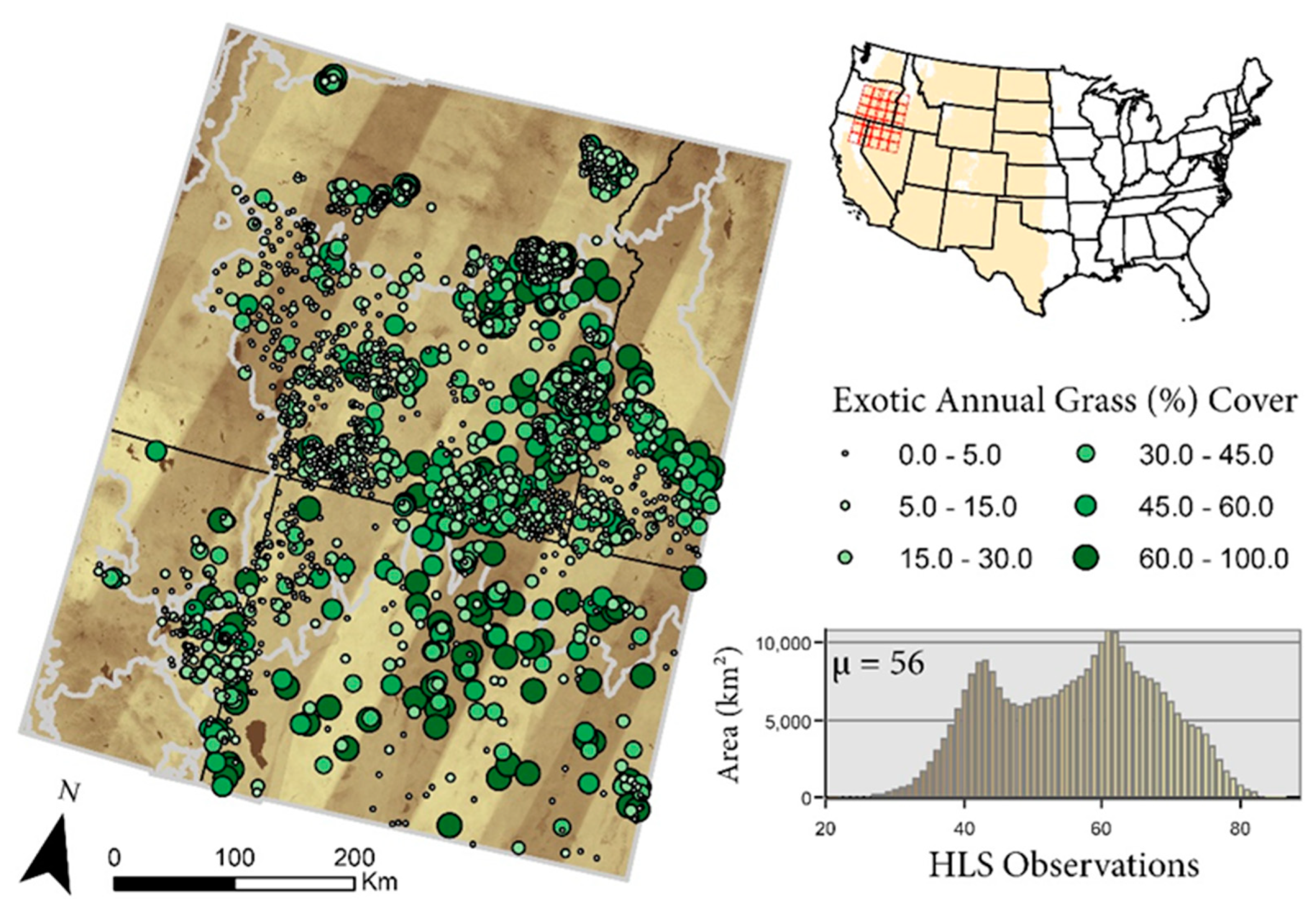
2.3. In Situ Observations of Exotic Annual Grass Cover, Modeling, and Map Validation

Field observations of exotic annual grass cover (2016–2017), the dominant component of which is assumed to be cheatgrass in our study area, were collected by the Bureau of Land Management (BLM) using a point-intercept approach along three-spoked (25 m) transects. Discrete point data taken along the BLM Assessment, Inventory, and Monitoring (AIM) transects were summarized to calculate the percent cover of exotic annual grasses for model calibration and validation (Figure 1; n = 1885). We compiled biophysical (i.e., Natural Resources Conservation Service Gridded Soil Survey Geographic (gSSURGO) [36] soil texture fraction and organic matter content in the first 30 cm of the soil; National Elevation Dataset (NED) [37]), and spectral data (Section 2.2) to serve as covariates within our predictive models because such factors are known to control or depict cheatgrass cover dynamics [11]. Spectral data were extracted coincident with the timing of the field observations (e.g., 2016 predictors extracted for 2016 in situ observations) because exotic annual grass cover can vary tenfold between wet and dry years [38,39] such as those evaluated in our study area (Figure S1).
We normalized the distribution of observations by percentage cover using a boot-strapping approach, where we reshuffled the model database while undersampling (retaining) those plots with zero (greater than zero) coverage of exotic annual grass cover, because of the prevalence of zero percent exotic annual grass cover observations in the field database. We then developed parsimonious regression tree models (n = 10) that were optimized using f-fold cross validation and the resampled databases from 2016–2017. Regression tree ensembles were constructed using an open-source version (GNU) of Cubist software and relevant environmental covariates as determined using tree-based feature selection algorithms and importance weights in sequential models. We performed a sensitivity analysis using different sets of NDVI composites (i.e., week + phenometrics, month, season, annual) to identify the optimal number and frequency of remote sensing inputs. We reported cross validation errors for each model and standard accuracy metrics across the study domain. The calibrated distribution models were then used to predict cheatgrass fractional cover for each permutation. Finally, we computed the pixel-wise median, standard deviation, and 2.5 and 97.5 percentiles of annual grass cover among the suite of permutations. This yielded both a best estimate (median) and 95% confidence interval for exotic annual grass cover at 30 m resolution for the study domain for all 3 years and the resulting maps were validated using independent observations (n = 112) distributed throughout the spatiotemporal domain.

3. Results

3.1. Image Masking and Validation

Manual image interpretations and classification tree output comparisons were favorable (Table 1), with mean overall accuracies of 85 ± 2% and 81 ± 2% for Landsat-8 and Sentinel-2 imagery, respectively. Standard HLS masks had slightly lower overall accuracies of 83% ± 2% and 78% ± 2% for Landsat-8 and Sentinel-2 imagery, respectively (Table 1). Mean overall accuracies within areas of model disagreement suggest a 50% overall increase in model accuracies when comparing independent interpretations to decision tree models (overall accuracy = 77 ± 7%) and standard HLS (38 ± 9%) masks. While a limited amount of independent test data was used in this comparison, this demonstrates that optimized, semi-supervised classification models significantly enhance our ability to distinguish clear and non-clear data within our study area.

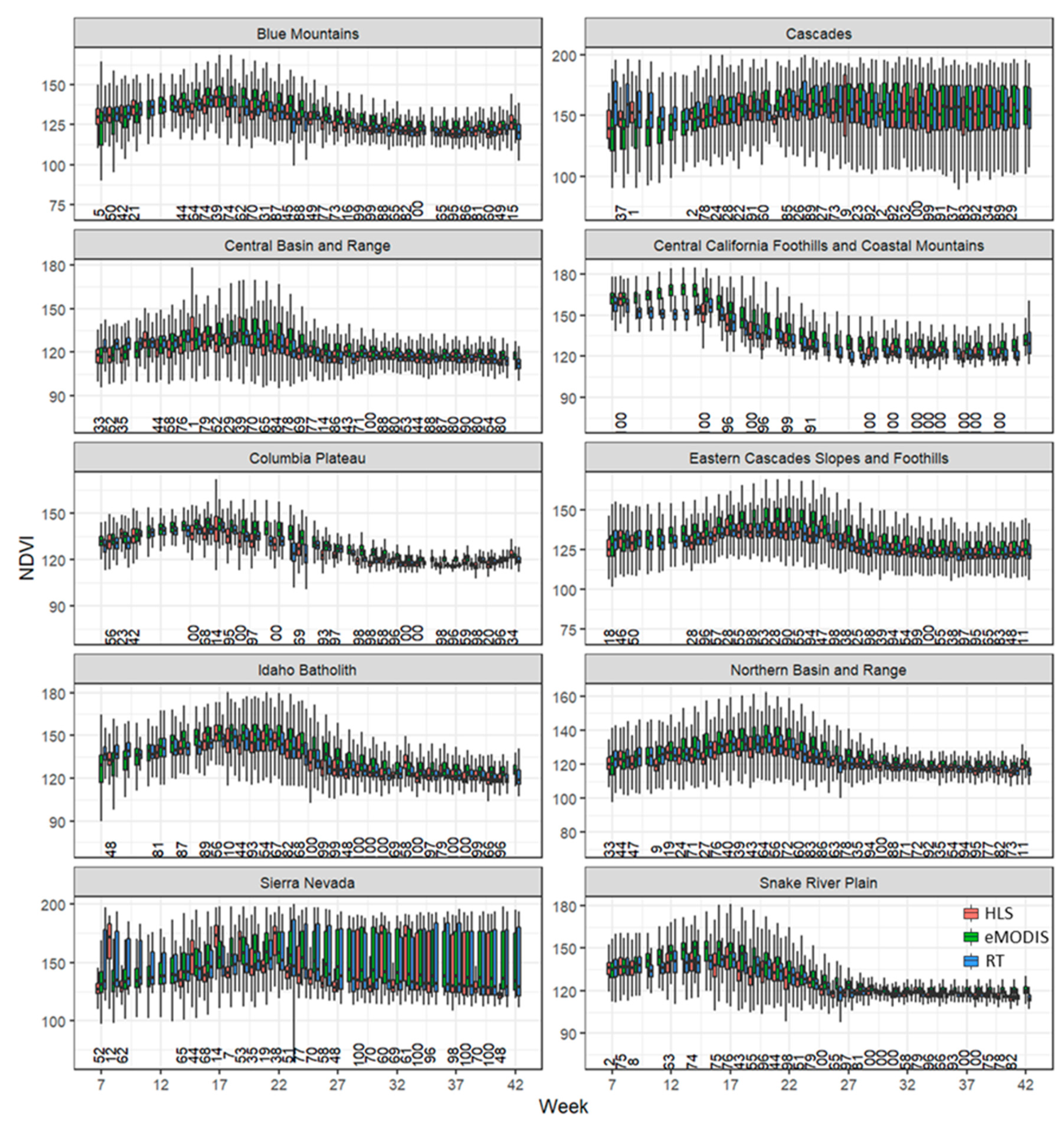
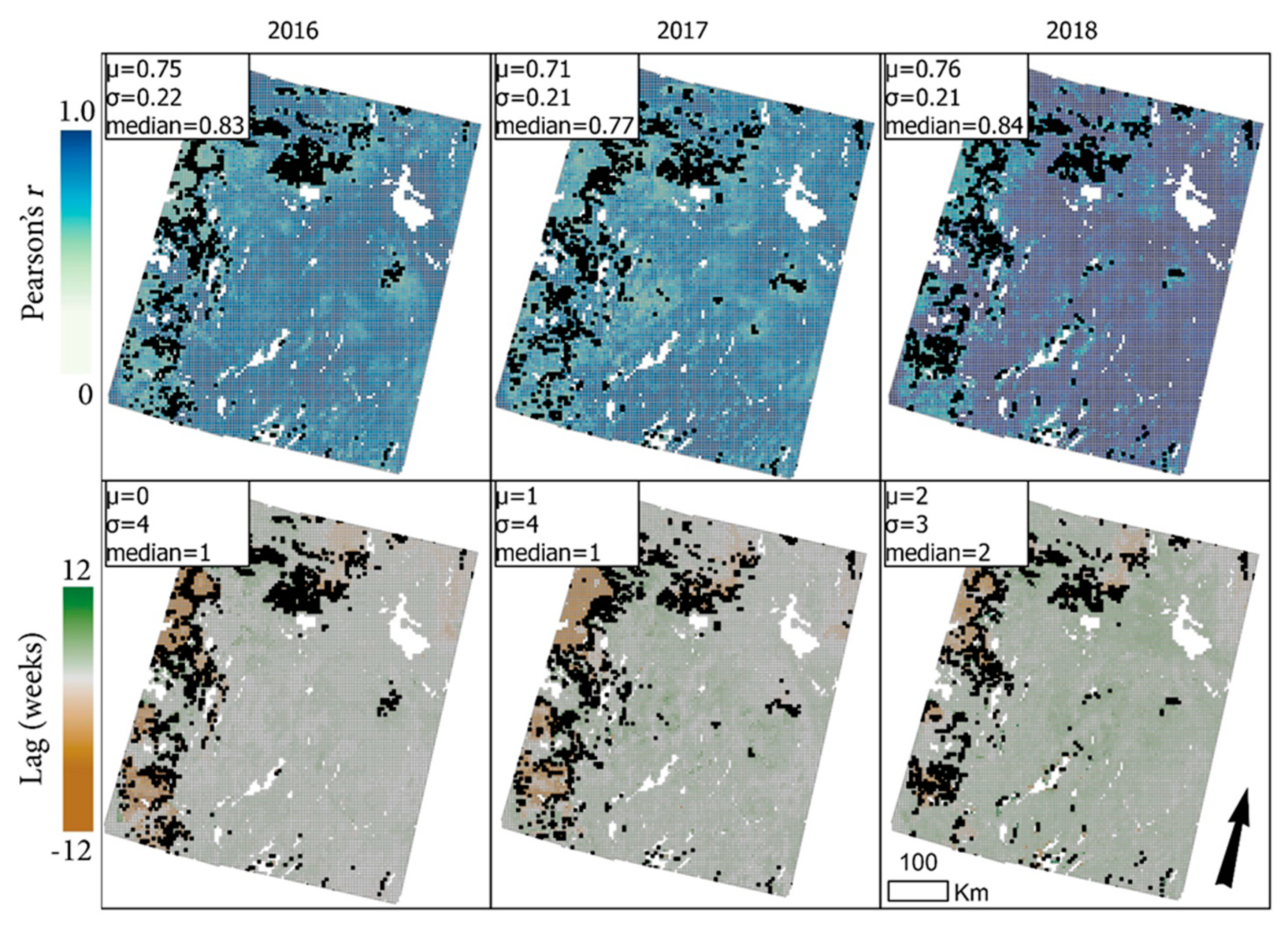
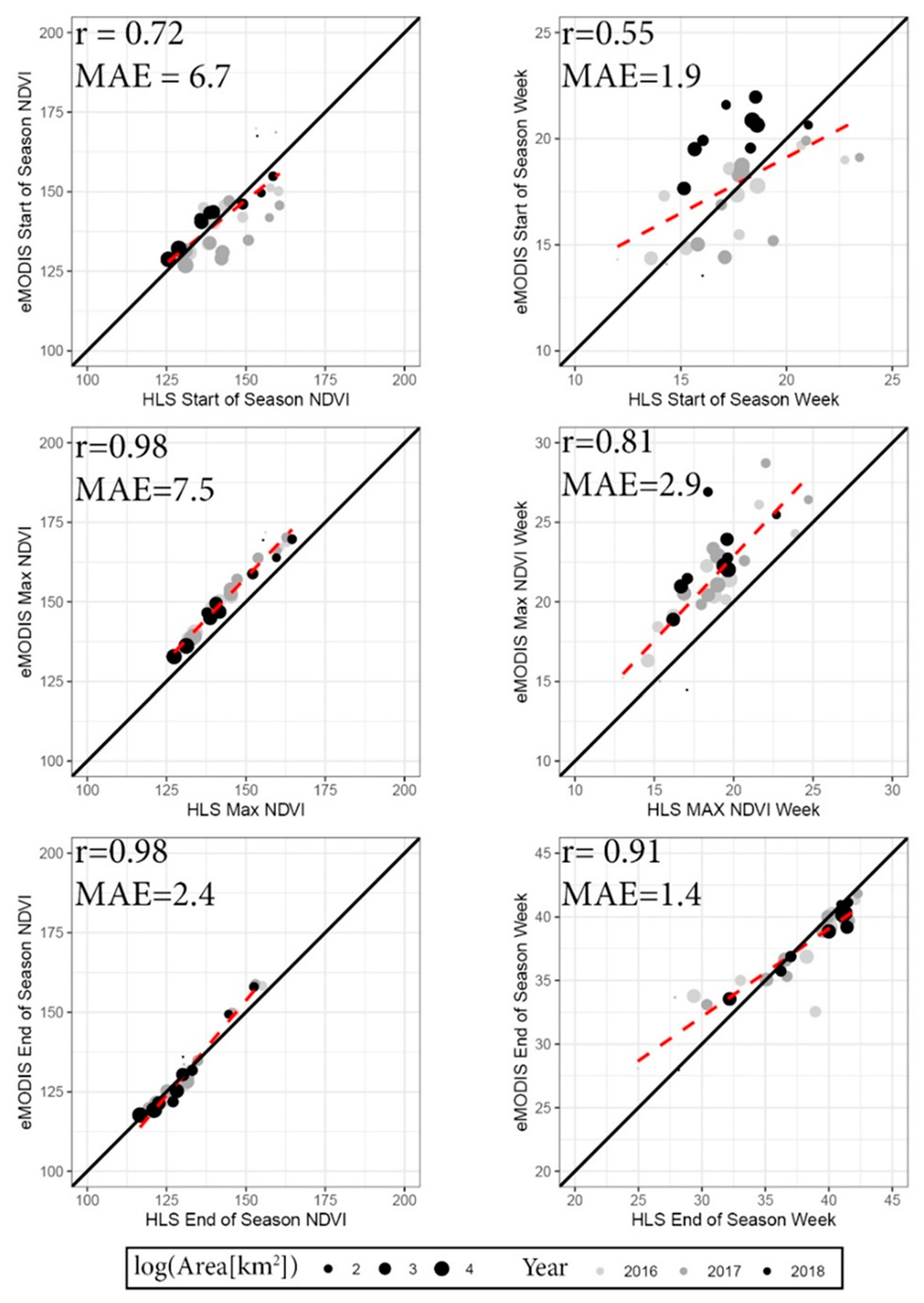
3.2. Time-Series Modeling and Metrics

The use of regression tree ensembles for spatiotemporal interpolation of spectral information is straightforward to implement and results in very high accuracies from the perspective of hold-out spectral data (Table S1). A paucity of observations, specifically long-term data gaps, result in increased error rates when using simpler smoothing methods, as compared to estimates made by complex regression tree models, which strongly influence the ultimate determination of phenological metrics and fractional exotic annual grass cover at a pixel (Figure 2). In dryland ecosystems, inter-annual variability of vegetation productivity distinct from land cover change is prominent in rangelands dominated by cheatgrass because of its link to rainfall [26,40]. Overall, we found stronger correlations between HLSRT and eMODIS data as compared to eMODIS and HLSint data (Table 2) generated using per-pixel compositing methods that are often used to construct cloud-free time-series data for input into models of land surface phenology or land cover change (e.g., [33,41]).
Cross-correlation analysis of eMODIS and HLSRT time-series data revealed good agreement between the datasets across evergreen forests and rangelands within the study area (Figure 3; average r = 0.74 ± 0.21; n = ~36,000), despite differences in how snow was handled in each time series (i.e., masked out in the HLS time series), with an average lag of 1 week between the time series (eMODIS lagging HLS data). Inclusion of snow-impacted pixels in MODIS time series can adversely impact start of season estimates within coniferous forests that typically have little inter-annual variation in NDVI [42] and are commonly found in western ecoregions of the study area (e.g., Cascades, Sierra Nevada), hence the reason for the exclusion of snow in the HLS dataset. Correspondingly, cross-correlation analysis indicates better agreement for years with relatively less precipitation (i.e., 2016 and 2018; Figure S1), despite the lack of Sentinel-2B observations in 2016, and within homogeneous rangelands less impacted by snow (r = 0.91; Table 2). For comparison, Robinson et al. [43] used a per-pixel and climatology-driven approach to produce 16-day Landsat composites and found a lower correspondence with MODIS data within homogenous evergreen forests and shrublands (average r = ~0.65) within the conterminous United States (1984–2016). Enhanced estimates of inter-annual NDVIs in the current study are mainly attributed to shorter revisit times of HLS data, the robust regression tree compositing and masking approach used here, and/or the known spatial inaccuracies of climatology data previously used for aiding interpolations of Landsat NDVI data.
Robust estimates of inter-annual variations in NDVI are a prerequisite for estimating phenological transition dates (phenophases), such as the start of the growing season. Comparisons between phenometrics derived from HLSRT and eMODIS data suggest further agreement between seasonal trajectories of NDVI across the spatial domain (Figure 4). For example, estimated mean start of season, maximum, and end of season NDVI values show good agreement with eMODIS-derived data, with Pearson’s correlation, and mean absolute errors (MAEs) ranging from 0.72 to 0.98 and from 0.02 to 0.08, respectively. Estimated timings followed similar patterns, with HLS-derived metrics generally indicating earlier start of season, maximum, and end of season timings as compared to eMODIS which is generally consistent with previous interpretations [32]. For comparison, Zhou et al. [44] used a weighted least-squares approach for temporal smoothing of HLS data and a delayed moving average technique to estimate the start of season date in grasslands along the eastern border of North Dakota and western Minnesota, with much higher data densities as compared to this study, and found fair agreement with MODIS-derived date estimates (RMSE = 11.6 days).

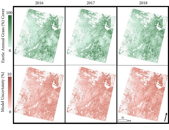
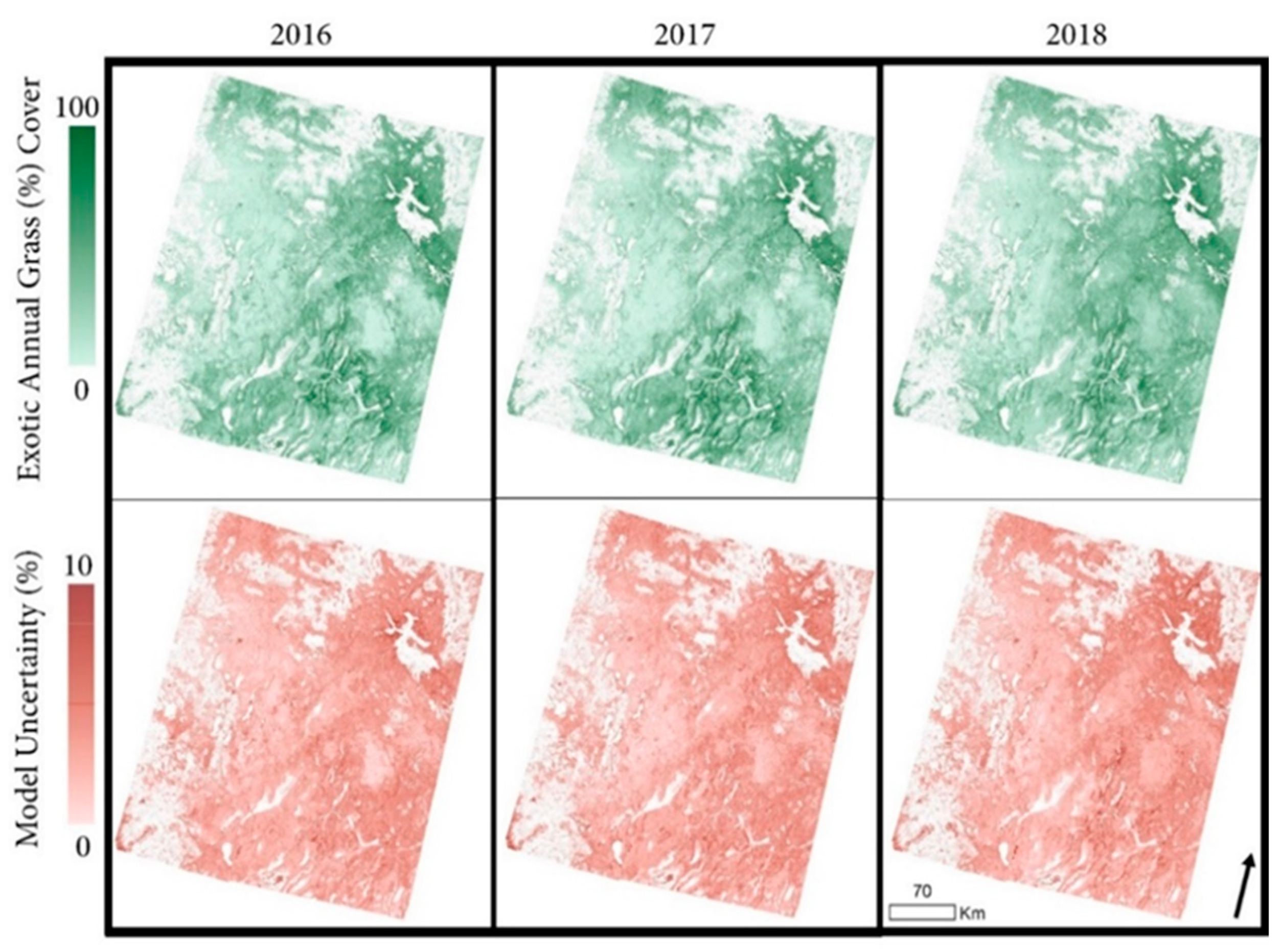
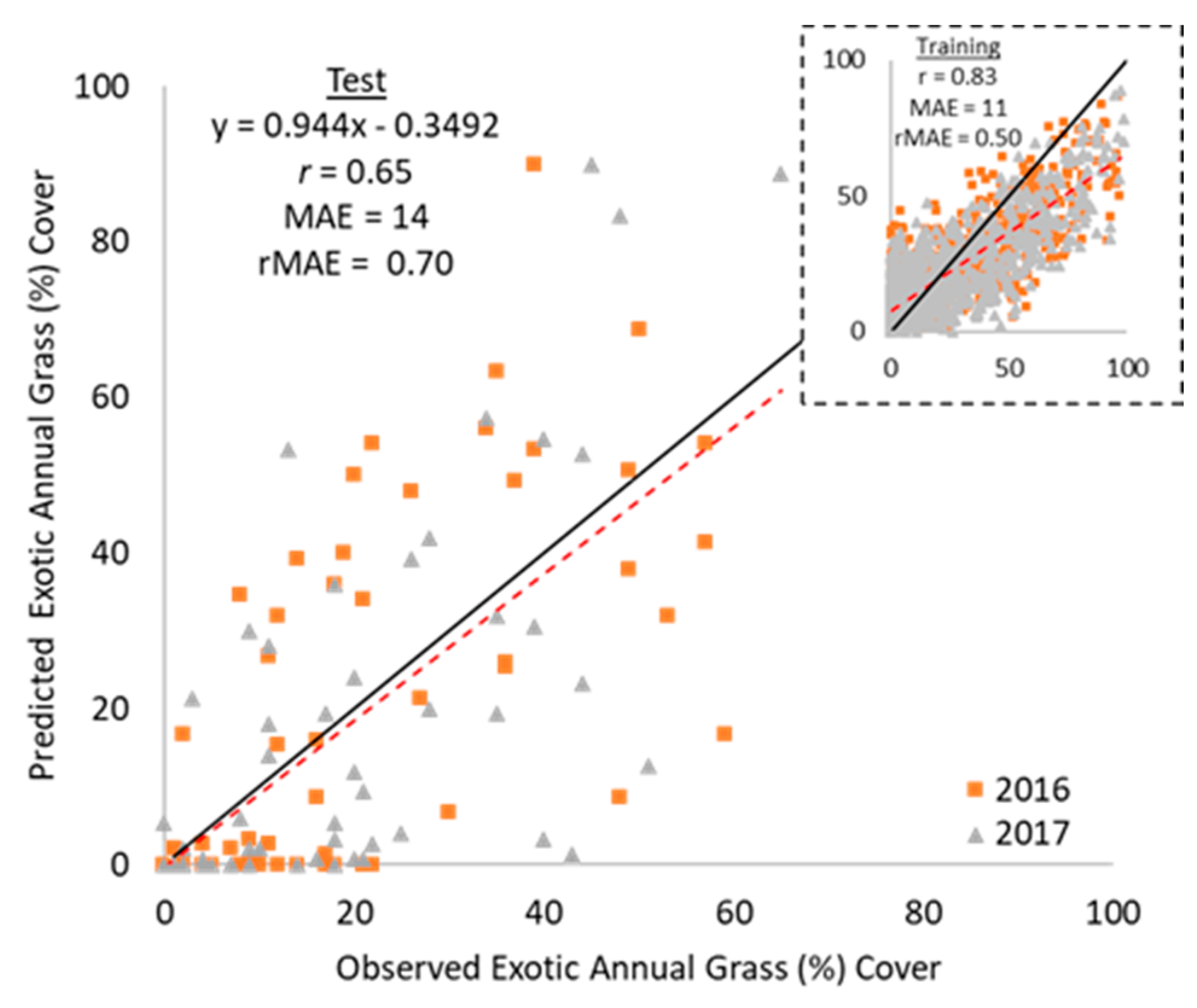
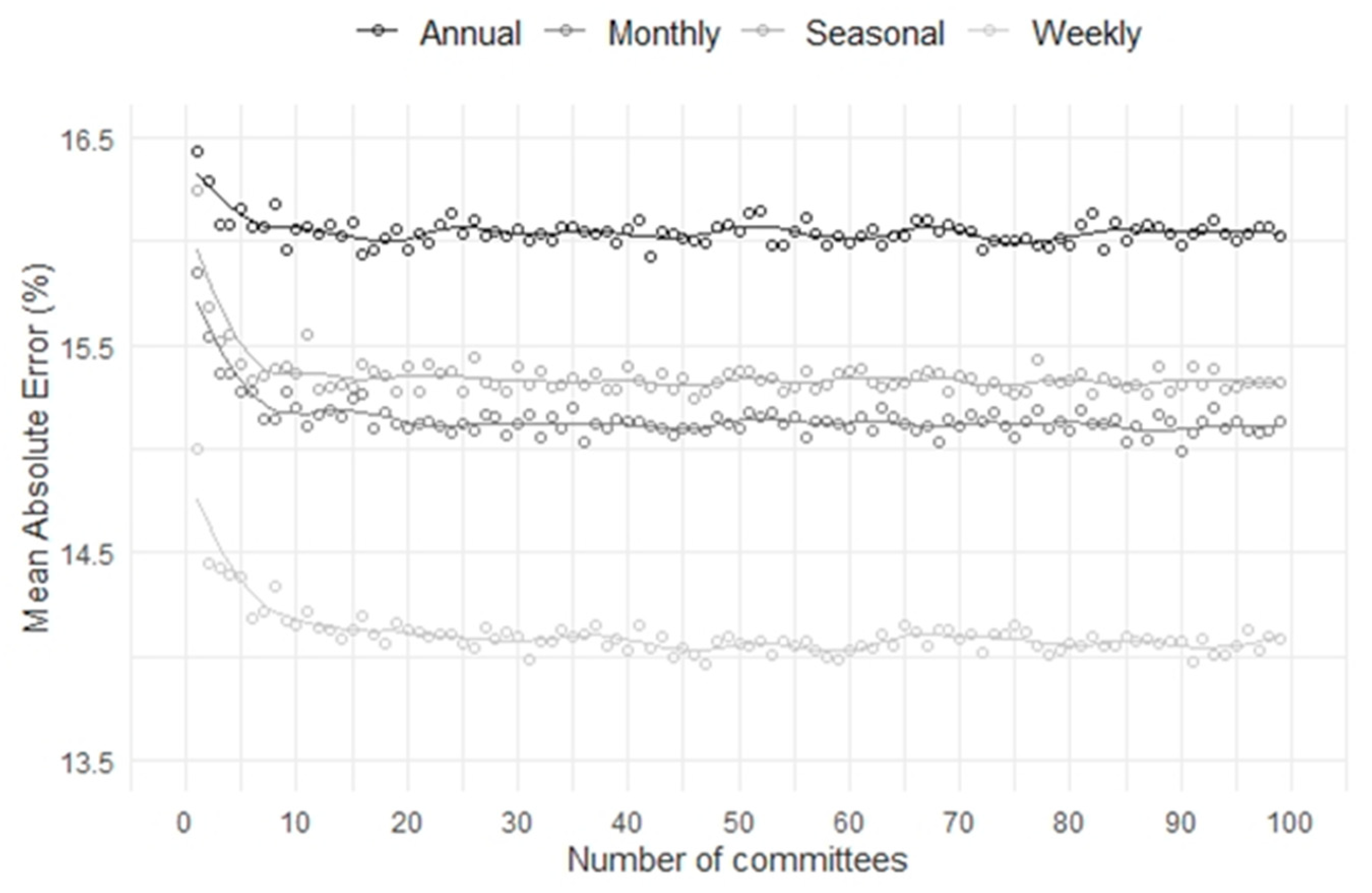
3.3. Exotic Annual Grass Cover Modeling, Mapping, and Validation

Our automated workflow produced exotic annual grass (%) cover maps (2016–2018) and associated estimates of model variance at 30-m spatial resolution across the study domain (Figure 5). Training and testing Pearson’s correlation coefficient (0.83 and 0.64), MAE (11% and 14% cover), and relative MAE (rMAE; 0.50 and 0.70) indicate fair agreement between modeled and observed percent cover values (Figure 6). These errors are either substantially lower or equivalent to those found in similar mapping efforts. For example, Jones et al. [15] generated estimates of annual, fractional forb, and grass cover using a random forest model that integrated some 30,000 field observations, seasonal Landsat image composites (1984 to 2017), and maps of abiotic and climatic factors and reported lower correlations between modeled and observed values when using out-of-bag summaries (r = 0.70) and independent test data (r = 0.44). Likewise, Xian and colleagues [16] used a regression tree model and Landsat Operational Land Imager (OLI) mosaics and reported fair (r = 0.56) agreement between independent field observations and model estimates of annual herbaceous cover. Similar levels of agreement (r = 0.50) were found when comparing 250-m annual invasive herbaceous cover maps, as derived from a regression tree model that used remotely sensed estimates of invasive annual herbaceous cover as model training data and MODIS data as a predictor, with six years of independent AIM plot data, despite large discrepancies in the scale of the AIM plots and spatial inputs [18].
Model variances were significantly associated with plotted and mapped cover values in our study (p-value < 0.01; r = 0.61; slope = 0.06; Figure 5), and partially attributed to positively skewed observation distributions [15], despite the data normalization and boot-strap approach used here. However, shuffling the model training data while undersampling the lower bounds of the data had a bias-reducing effect as compared to nonparametric modeling schemes that did not assign weights to rarer observations (e.g., [15,46]). Similarly, Henderson and colleagues [14] used a probability-based threshold and linear correction procedure in a univariate random forest modeling scheme, which required accurate and unbiased presence-absence/probability models developed for a user-defined threshold of cover, to construct relatively unbiased estimates of annual invasive grass cover in a portion of the Great Basin.
The robustness of our distribution model was largely contingent upon the number and quality of the ground truth data, which should be collected at scales congruent with remote sensing inputs, and the predictive capacity of the environmental covariates. Sensitivity analysis revealed that models which made use of weekly NDVI composites and phenometrics significantly outperformed those that made use of monthly, seasonal, or annual image composites and ancillary data (Figure 7). This finding suggests that the temporal granularity of the remote sensing inputs significantly controls the accuracy of the species distribution models, with the timing of key phenological transitions (e.g., start of green-up and brown-down) and associated weekly spectral values being heavily used across model development (Table S2).

4. Discussion

4.1. Time Series Modeling, Metrics, and Image Masking

Remote sensing of vegetation productivity and land surface phenology in dryland ecosystems can be immensely challenging due to pervasive cloudiness during spring months, high amounts of bare ground and biological soil crusts, high spatial heterogeneity, low vegetation signal-to-noise ratios, and irregular growing seasons related to seasonal rainfall and frequent periods of drought [47]. To circumvent data availability and scaling issues, we developed a data fusion approach that leveraged HLS data (i.e., Sentinel-2A and B, Landsat 8) and machine-learning techniques to construct weekly, cloud-free NDVI image composites for an accurate representation of seasonal cycles of vegetation greenness and estimates of phenological transition dates. Identification of clear and non-clear pixel data (i.e., data quality screening) is a prerequisite for any satellite-based remote sensing analysis and the use of optimized decision tree models resulted in improved accuracies as compared to standard HLS masks in this study (Table 1). We suspect the standard HLS masks represent a more global solution based on a physics-based pixel quality identification while our semi-supervised approach allows for scene and date-specific tuning for improved cloud, shadow, water, and snow/ice identification. It is important to note, however, that cloud and cloud shadow detection algorithms were recently improved for Landsat and Sentinel-2 data (Fmask 4.0; [48]) and such data can easily be assimilated into our workflow in the future.
We demonstrate that our regression tree compositing method is more robust than per-pixel approaches that are typically used to construct time-series data for input into models of land surface phenology or land cover change (Figure 2 and Table 2). A key advantage of using a global versus pixel-based modeling scheme is the ability to leverage data across the spatiotemporal domain, as opposed strictly to the temporal domain, to make predictions at each pixel and time step. While our approach was mainly developed for monitoring precipitation-driven ecosystems with abrupt and flashy growth cycles, it is transferable to more temperature-driven ecosystems where vegetation synchronizes its growth with relatively consistent seasonal climatic changes using environmental cues (e.g., temperature, photoperiod). Regardless, when insufficient high-quality data are available for training during the beginning and end of the growing season, or when there are high levels of undetected noise in the data (e.g., due to inaccurate masking algorithms), the resulting function fits can still be unrealistic and may require further processing or filtering (e.g., Savitzky–Golay filter, Hampel filter) to diminish noise or artifacts. Since the advancement of remote sensing of land surface phenology is vital for better understanding drylands [49], future research should explore the benefits of using an ensemble of methodologies and spectral indices (e.g., Soil-Adjusted Vegetation Index) to characterize phenological timings (e.g., [50]), leverage residuals from curve fitting procedures to calculate measures of statistical uncertainty in the phenophases dates and associated spectral values, and make comparisons with ground-based optical measurements acquired at scales commensurate with remote sensing inputs.

4.2. Exotic Annual Grass Cover Modeling, Mapping, and Validation

Our automated workflow produced maps of exotic annual grass (%) cover associated estimates of model variance throughout dryland ecosystems of the western United States at a native, 30-m spatial resolution. Comparisons with independent field observations and error assessments reported in previous studies suggest improved accuracies that can be partially attributed to: (1) the enhanced temporal revisit times and resolutions of the HLS dataset, which allowed for the development of nearly seamless weekly NDVI data (Figure 7); (2) consistent usage of sampling protocols across the model testing and training datasets; and/or (3) the use of other relevant ancillary data related to exotic annual grass cover (i.e., phenometrics, soils, topography). Moreover, while there are existing systems that use multi-date satellite imagery to develop fractional cover maps of annual invasive herbaceous cover [19,21,51], such approaches are generally not suited for developing near real-time estimates. These approaches, which are subject to data latency issues or a lack of an automated workflow, have made use of coarse spatial-resolution inputs (e.g., eMODIS), downscaled MODIS products, or composites constructed from Landsat data with coarse temporal granularity (i.e., 16 day), and have not capitalized on the synergistic use of seamless Landsat-8 and Sentinel-2 data for improved characterization of invasive annual grass dynamics.
With regards to scaling issues and sampling errors, we opportunistically used BLM AIM plot data that were not optimally aligned with the scale of the remote sensing inputs and were collected using point-intercept sampling rather than a complete enumeration/inventory with no sampling errors. To circumvent scaling issues, we initially gave higher weights to observations that fell within relatively homogenous areas, as identified by calculating the coefficient of variation of growing season NDVI data within a 3 × 3 moving window, but this did not improve model accuracies from the perspective of hold-out data. Likewise, previous research has shown that it can be important to train machine-learning models on mixed pixels that can occupy a large portion of the spatiotemporal domain [52]. Future studies may benefit by tackling scaling issues in other ways; for example, by upscaling more localized in situ observations (with no sampling errors) using high-resolution imagery collected via suborbital (e.g., unmanned aerial vehicle (UAV)) or orbital (e.g., CubeSat, DigitalGlobe) sensors, and then using those estimates as training data within distribution models that use moderate-resolution imagery inputs (e.g., [48]) while also tracking uncertainties throughout the entire prediction process.

5. Conclusions

In this study, we developed a fully automated and scalable workflow that integrates field observations, harmonized Landsat and Sentinel-2 (HLS) data, maps of landscape conditions (i.e., soils, topography), and machine-learning techniques to construct a time series of fractional estimates of exotic annual grass cover and associated uncertainties across dryland ecoregions in the western United States [53]. In doing so, we also show that Landsat 8 and Sentinel-2 data can be used in harmony to generate weekly cloud-free image composites of NDVI data and estimates of phenological transition dates comparable to those derived from eMODIS data but at scales (30 m) more relevant to local resource managers. The development and public release of spatially explicit maps of exotic annual grass (%) cover and weekly NDVI can be important assets to land managers and scientists. This workflow and derived information will be immensely useful for numerous science activities and investigations such as monitoring and modeling historical and future land-surface dynamics and biophysical conditions (e.g., biomass, drought), detecting and analyzing fuel breaks in sagebrush ecosystems [54], controlling and quantifying fire behavior, targeting grazing, mapping other rangeland components (e.g., % bare ground, shrubs, herbs), and enhancing aerial herbicide applications. Timely, accurate, and spatially detailed depictions of land surface phenology and exotic annual grass cover serve as foundations for better understanding and managing dryland systems in the face of a changing climate and disturbance regimes.

Supplementary Materials

The following are available online at https://0-www-mdpi-com.brum.beds.ac.uk/2072-4292/12/4/725/s1, Figure S1: Time series of mean annual precipitation (mm) anomalies for level III ecoregions (Omernik and Griffith, 2014), Table S1: Average statistical metrics (±SD) derived from observed and predicted normalized difference vegetation index (NDVI * 100) values (2016–2018), Table S2: Predictor variable usage (+SD) across 10 regression tree (RT) models developed.

Author Contributions

N.J.P. and B.K.W. conceived and designed the study. N.J.P. wrote the original manuscript. D.D. and S.P. were responsible for automating a large portion of the data processing workflow with input from N.J.P. and B.K.W, and lastly, S.P.B. and Z.W. contributed to scientific writing and interpretations. All authors have read and agree to the published version of the manuscript.

Funding

This research was funded by the U.S. Geological Survey’s National Land Imaging and Land Change Science Programs, the Bureau of Land Management (RU16PWF0008), and the Fish and Wildlife Service (4500110419). A portion of the work was performed under USGS contract G15PC00012.

Acknowledgments

We thank Matthew B. Rigge and anonymous reviewers for comments on earlier versions of this manuscript. Any use of trade, firm, or product names is for descriptive purposes only and does not imply endorsement by the U.S. Government.

Conflicts of Interest

The authors declare no conflicts of interest.

References

  1. Fusco, E.J.; Finn, J.T.; Balch, J.K.; Nagy, R.C.; Bradley, B.A. Invasive grasses increase fire occurrence and frequency across US ecoregions. Proc. Natl. Acad. Sci. USA 2019, 116, 23594–23599. [Google Scholar] [CrossRef]
  2. Balch, J.K.; Bradley, B.A.; D’Antonio, C.M.; Gomez-Dans, J. Introduced annual grass increases regional fire activity across the arid western USA (1980-2009). Glob. Chang. Biol. 2013, 19, 173–183. [Google Scholar] [CrossRef] [PubMed]
  3. Bradley, B.A.; Houghton, R.A.; Mustard, J.F.; Hamburg, S.P. Invasive grass reduces aboveground carbon stocks in shrublands of the Western US. Glob. Chang. Biol. 2006, 12, 1815–1822. [Google Scholar] [CrossRef] [Green Version]
  4. Chambers, J.C. Collaborative management and research in the Great Basin—Examining the issues and developing a framework for action. In Invasive Plant Species and the Great Basin; U.S. Department of Agriculture, Forest Service, Rocky Mountain Research Station: Fort Collins, CO, USA, 2008; pp. 38–41. [Google Scholar]
  5. Mack, R.N.; Pyke, D.A. The demography of Bromus Tectorum: Variation in time and space. J. Ecol. 1983, 71, 69–93. [Google Scholar] [CrossRef]
  6. Compagnoni, A.; Adler, P.B. Warming, competition, and Bromus tectorum population growth across an elevation gradient. Ecosphere 2014, 5, art121. [Google Scholar] [CrossRef]
  7. Chambers, J.C.; Roundy, B.A.; Blank, R.R.; Meyer, S.E.; Whittaker, A. What makes Great Basin sagebrush ecosystems invasible by Bromus tectorum? Ecol. Monogr. 2007, 77, 117–145. [Google Scholar] [CrossRef] [Green Version]
  8. Boyte, S.P.; Wylie, B.K.; Major, D.J. Cheatgrass percent cover change: Comparing recent estimates to climate change−driven predictions in the northern Great Basin. Rangel. Ecol. Manag. 2016, 69, 265–279. [Google Scholar] [CrossRef]
  9. Bradley, B.A.; Curtis, C.A.; Chambers, J.C. Bromus Response to Climate and Projected Changes with Climate Change. In Exotic Brome-Grasses in Arid and Semiarid Ecosystems of the Western US; Germino, M.J., Chambers, J.C., Brown, C.S., Eds.; Springer International Publishing: Cham, Switzerland, 2016; pp. 257–274. ISBN 978-3-319-24928-5. [Google Scholar]
  10. Abatzoglou, J.T.; Kolden, C.A. Climate Change in Western US Deserts: Potential for Increased Wildfire and Invasive Annual Grasses. Rangel. Ecol. Manag. 2011, 64, 471–478. [Google Scholar] [CrossRef]
  11. Chambers, J.C.; Bradley, B.A.; Brown, C.S.; D’Antonio, C.; Germino, M.J.; Grace, J.B.; Hardegree, S.P.; Miller, R.F.; Pyke, D.A. Resilience to Stress and Disturbance, and Resistance to Bromus tectorum L. Invasion in Cold Desert Shrublands of Western North America. Ecosystems 2014, 17, 360–375. [Google Scholar] [CrossRef]
  12. Bradley, B.A.; Mustard, J.F. Characterizing the landscape dynamics of an invasive plant and risk of invasion using remote sensing. Ecol. Appl. 2006, 16, 1132–1147. [Google Scholar] [CrossRef] [Green Version]
  13. Hobbs, R.J.; Humphries, S.E. An integrated approach to the ecology and management of plant invasions. Conserv. Biol. 1995, 9, 761–770. [Google Scholar] [CrossRef] [Green Version]
  14. Henderson, E.B.; Bell, D.M.; Gregory, M.J. Vegetation mapping to support greater sage-grouse habitat monitoring and management: Multi- or univariate approach? Ecosphere 2019, 10, e02838. [Google Scholar] [CrossRef]
  15. Jones, M.O.; Allred, B.W.; Naugle, D.E.; Maestas, J.D.; Donnelly, P.; Metz, L.J.; Karl, J.; Smith, R.; Bestelmeyer, B.; Boyd, C.; et al. Innovation in rangeland monitoring: Annual, 30 m, plant functional type percent cover maps for U.S. rangelands, 1984-2017. Ecosphere 2018, 9, e02430. [Google Scholar] [CrossRef]
  16. Xian, G.; Homer, C.; Rigge, M.; Shi, H.; Meyer, D. Characterization of shrubland ecosystem components as continuous fields in the northwest United States. Remote Sens. Environ. 2015, 168, 286–300. [Google Scholar] [CrossRef] [Green Version]
  17. Bradley, B.A. Remote detection of invasive plants: A review of spectral, textural and phenological approaches. Biol. Invasions 2013, 16, 1411–1425. [Google Scholar] [CrossRef]
  18. Boyte, S.P.; Wylie, B.K. Near-real-time cheatgrass percent cover in the northern Great Basin, USA, 2015. Rangelands 2016, 38, 278–284. [Google Scholar] [CrossRef] [Green Version]
  19. Boyte, S.P.; Wylie, B.K.; Major, D.J. Mapping and monitoring cheatgrass dieoff in rangelands of the northern Great Basin, USA. Rangel. Ecol. Manag. 2015, 68, 18–28. [Google Scholar] [CrossRef]
  20. Weisberg, P.J.; Dilts, T.E.; Baughman, O.W.; Meyer, S.E.; Leger, E.A.; Van Gunst, K.J.; Cleeves, L. Development of remote sensing indicators for mapping episodic die-off of an invasive annual grass (Bromus tectorum) from the Landsat archive. Ecol. Indic. 2017, 79, 173–181. [Google Scholar] [CrossRef]
  21. West, A.M.; Evangelista, P.H.; Jarnevich, C.S.; Kumar, S.; Swallow, A.; Luizza, M.W.; Chignell, S.M. Using multi-date satellite imagery to monitor invasive grass species distribution in post-wildfire landscapes: An iterative, adaptable approach that employs open-source data and software. Int. J. Appl. Earth Obs. Geoinf. 2017, 59, 135–146. [Google Scholar] [CrossRef]
  22. Ibáñez, I.; Silander, J.A., Jr.; Allen, J.M.; Treanor, S.A.; Wilson, A. Identifying hotspots for plant invasions and forecasting focal points of further spread. J. Appl. Ecol. 2009, 46, 1219–1228. [Google Scholar] [CrossRef] [Green Version]
  23. Vilà, M.; Ibáñez, I. Plant invasions in the landscape. Landsc. Ecol. 2011, 26, 461–472. [Google Scholar] [CrossRef]
  24. Clinton, N.E.; Potter, C.; Crabtree, B.; Genovese, V.; Gross, P.; Gong, P. Remote sensing-based time-series analysis of cheatgrass (Bromus tectorum L.) phenology. J. Environ. Qual. 2010, 39, 955–963. [Google Scholar] [CrossRef] [PubMed]
  25. Singh, N.; Glenn, N.F. Multitemporal spectral analysis for cheatgrass (Bromus tectorum) classification. Int. J. Remote Sens. 2009, 30, 3441–3462. [Google Scholar] [CrossRef]
  26. Bradley, B.A.; Mustard, J.F. Identifying land cover variability distinct from land cover change: Cheatgrass in the Great Basin. Remote Sens. Environ. 2005, 94, 204–213. [Google Scholar] [CrossRef]
  27. Claverie, M.; Ju, J.; Masek, J.G.; Dungan, J.L.; Vermote, E.F.; Roger, J.-C.; Skakun, S.V.; Justice, C. The Harmonized Landsat and Sentinel-2 surface reflectance data set. Remote Sens. Environ. 2018, 219, 145–161. [Google Scholar] [CrossRef]
  28. Omernik, J.M.; Griffith, G.E. Ecoregions of the conterminous United States: Evolution of a hierarchical spatial framework. Environ. Manag. 2014, 54, 1249–1266. [Google Scholar] [CrossRef]
  29. Trabucco, A.; Zomer, R.J. Global Aridity Index (Global-Aridity) and Global Potential Evapo-Transpiration (Global-PET) Geospatial Database 2019. Available online: https://cgiarcsi.community/2019/01/24/global-aridity-index-and-potential-evapotranspiration-climate-database-v2/ (accessed on 1 December 2019).
  30. Quinlan, J.R. C4.5: Programs for Machine Learning; Morgan Kaufmann Publishers, Inc.: San Francisco, CA, USA, 1993; ISBN 978-1-55860-238-0. [Google Scholar]
  31. Congalton, R.G. A review of assessing the accuracy of classifications of remotely sensed data. Remote Sens. Environ. 1991, 37, 35–46. [Google Scholar] [CrossRef]
  32. Pastick, N.; Wylie, B.; Wu, Z. Spatiotemporal analysis of Landsat-8 and Sentinel-2 data to support monitoring of dryland ecosystems. Remote Sens. 2018, 10, 791. [Google Scholar] [CrossRef] [Green Version]
  33. Hughes, M.; Hayes, D. Automated detection of cloud and cloud shadow in single-date Landsat imagery using neural networks and spatial post-processing. Remote Sens. 2014, 6, 4907–4926. [Google Scholar] [CrossRef] [Green Version]
  34. Jenkerson, C.B.; Maiersperger, T.; Schmidt, G. eMODIS: A User-Friendly Data Source; Open-File Report; U.S. Geological Survey: Reston, VA, USA, 2010.
  35. Araya, S.; Ostendorf, B.; Lyle, G.; Lewis, M. CropPhenology: An R package for extracting crop phenology from time series remotely sensed vegetation index imagery. Ecol. Inform. 2018, 46, 45–56. [Google Scholar] [CrossRef]
  36. Soil Survey Staff. Gridded Soil Survey Geographic (gSSURGO) Database for the Conterminous United States 2019. Available online: https://nrcs.app.box.com/v/soils/folder/94124173798 (accessed on 1 December 2019).
  37. Gesch, D.B.; Evans, G.A.; Oimoen, M.J.; Arundel, S. The National Elevation Dataset; American Society for Photogrammetry and Remote Sensing: Bethesda, MD, USA, 2018; pp. 83–110. [Google Scholar]
  38. Hull, A.C.; Pechanec, J.F. Cheatgrass: A challenge to range research. J. For. 1947, 45, 555–564. [Google Scholar]
  39. Stewart, G.; Hull, A.C. Cheatgrass (Bromus Tectorum L.)—An ecologic intruder in southern Idaho. Ecology 1949, 30, 58–74. [Google Scholar] [CrossRef]
  40. Rigge, M.; Shi, H.; Homer, C.; Danielson, P.; Granneman, B. Long-term trajectories of fractional component change in the Northern Great Basin, USA. Ecosphere 2019, 10, e02762. [Google Scholar] [CrossRef]
  41. White, J.C.; Wulder, M.A.; Hobart, G.W.; Luther, J.E.; Hermosilla, T.; Griffiths, P.; Coops, N.C.; Hall, R.J.; Hostert, P.; Dyk, A.; et al. Pixel-based image compositing for large-area dense time series applications and science. Can. J. Remote Sens. 2014, 40, 192–212. [Google Scholar] [CrossRef] [Green Version]
  42. Gamon, J.A.; Huemmrich, K.F.; Wong, C.Y.S.; Ensminger, I.; Garrity, S.; Hollinger, D.Y.; Noormets, A.; Peñuelas, J. A remotely sensed pigment index reveals photosynthetic phenology in evergreen conifers. Proc. Natl. Acad. Sci. USA 2016, 113, 13087. [Google Scholar] [CrossRef] [PubMed] [Green Version]
  43. Robinson, P.N.; Allred, W.B.; Jones, O.M.; Moreno, A.; Kimball, S.J.; Naugle, E.D.; Erickson, A.T.; Richardson, D.A. A Dynamic Landsat Derived Normalized Difference Vegetation Index (NDVI) Product for the Conterminous United States. Remote Sens. 2017, 9, 863. [Google Scholar] [CrossRef] [Green Version]
  44. Zhou, Q.; Rover, J.; Brown, J.; Worstell, B.; Howard, D.; Wu, Z.; Gallant, L.A.; Rundquist, B.; Burke, M. Monitoring Landscape Dynamics in Central U.S. Grasslands with Harmonized Landsat-8 and Sentinel-2 Time Series Data. Remote Sens. 2019, 11, 328. [Google Scholar] [CrossRef] [Green Version]
  45. Yang, L.; Jin, S.; Danielson, P.; Homer, C.; Gass, L.; Bender, S.M.; Case, A.; Costello, C.; Dewitz, J.; Fry, J.; et al. A new generation of the United States National Land Cover Database: Requirements, research priorities, design, and implementation strategies. ISPRS J. Photogramm. Remote Sens. 2018, 146, 108–123. [Google Scholar] [CrossRef]
  46. Homer, C.G.; Aldridge, C.L.; Meyer, D.K.; Schell, S.J. Multi-scale remote sensing sagebrush characterization with regression trees over Wyoming, USA: Laying a foundation for monitoring. Int. J. Appl. Earth Obs. Geoinf. 2012, 14, 233–244. [Google Scholar] [CrossRef]
  47. Smith, W.K.; Dannenberg, M.P.; Yan, D.; Herrmann, S.; Barnes, M.L.; Barron-Gafford, G.A.; Biederman, J.A.; Ferrenberg, S.; Fox, A.M.; Hudson, A.; et al. Remote sensing of dryland ecosystem structure and function: Progress, challenges, and opportunities. Remote Sens. Environ. 2019, 233, 111401. [Google Scholar] [CrossRef]
  48. Qiu, S.; Zhu, Z.; He, B. Fmask 4.0: Improved cloud and cloud shadow detection in Landsats 4–8 and Sentinel-2 imagery. Remote Sens. Environ. 2019, 231, 111205. [Google Scholar] [CrossRef]
  49. Ganguly, S.; Friedl, M.A.; Tan, B.; Zhang, X.; Verma, M. Land surface phenology from MODIS: Characterization of the Collection 5 global land cover dynamics product. Remote Sens. Environ. 2010, 114, 1805–1816. [Google Scholar] [CrossRef] [Green Version]
  50. White, M.A.; De Beurs, K.M.; Didan, K.; Inouye, D.W.; Richardson, A.D.; Jensen, O.P.; O’Keefe, J.; Zhang, G.; Nemani, R.R.; Van Leeuwn, W.J.D.; et al. Intercomparison, interpretation, and assessment of spring phenology in North America estimated from remote sensing for 1982–2006. Glob. Chang. Biol. 2009, 15, 2335–2359. [Google Scholar] [CrossRef]
  51. Kokaly, R.F. Detecting Cheatgrass on the Colorado Plateau Using Landsat Data: A Tutorial for the DESI Software; Open-File Report; U.S. Geological Survey: Reston, VA, USA, 2011.
  52. Hansen, M.C. Classification Trees and Mixed Pixel Training Data. In Remote Sensing of Land Cover: Principles and Applications; Chandra, G., Ed.; Taylor and Francis: New York, NY, USA, 2012. [Google Scholar]
  53. Dahal, D.; Wylie, B.K.; Parajuli, S.; Pastick, N.J. Fractional Estimates of Invasive Annual Grass cover in Dryland Ecosystems of Western United States (2016–2018); U.S. Geological Survey: Reston, VA, USA, 2020.
  54. Shinneman, D.J.; Germino, M.J.; Pilliod, D.S.; Aldridge, C.L.; Vaillant, N.M.; Coates, P.S. The ecological uncertainty of wildfire fuel breaks: Examples from the sagebrush steppe. Front. Ecol. Environ. 2019, 17, 279–288. [Google Scholar] [CrossRef]
Figure 1. Number of valid harmonized Landsat and Sentinel-2 (HLS) observations from 2016 to 2018 overlaid by level III ecoregions [28] and Bureau of Land Management Assessment, Inventory, and Monitoring (AIM) plots (2016–2017). Black lines indicate state boundaries and inset shows Sentinel-2 tiles and drylands in the United States. Drylands are defined by an aridity index [29], where the average ratio of annual precipitation to potential evapotranspiration (1970 to 2000) is between 0.03 and 0.5.
Remotesensing 12 00725 g001
Figure 2. Time series of Normalized Difference Vegetation Index (NDVI) derived from harmonized Landsat and Sentinel-2 (HLS) data, regression tree models, and expediated Moderate Resolution Image Spectroradiometer (eMODIS) dataset within rangelands stratified by level III ecoregions [28]. The box plots show the interquartile range and median weekly NDVI values (horizontal black line) in 2016. The whiskers extend to a range of values that are within the median ± 1.5 times the interquartile range. HLS data coverage (%) is displayed at the bottom of each panel and rounded to the nearest whole number. NDVI is scaled (100× + 100) to an 8-bit unsigned integer.
Remotesensing 12 00725 g002
Figure 3. Cross-correlation and lag statistics between eMODIS and regression tree estimated Normalized Difference Vegetation Index (NDVI) as summarized across all 5 × 5 km grids during 2016–2018. Time series were populated using NDVI values within target land cover types (i.e., rangelands and evergreen forests). Areas with insignificant correlations (p-value > 0.05) and mostly non-target land covers are shown as black and white grids, respectively. A positive (negative) lag indicates that eMODIS NDVI lags (leads) that of HLSRT NDVI.
Remotesensing 12 00725 g003
Figure 4. Mean satellite-derived phenophase metrics and associated Normalized Difference Vegetation Index (NDVI) for rangelands stratified by level III ecoregions [28] over the 2016–2018 record. Phenometrics are summarized for homogeneous pixels (coefficient of variation <20%), as calculated from standard deviation and mean focal scans (9 × 9 pixels) of the average 30-m growing season NDVI, as estimated from regression tree models. Pearson’s correlation coefficient (r) and mean absolute error (MAE) are shown for all years combined. Data were fit using ordinary least-squares regression (dashed line) and the 1:1 line is shown as a solid black line. NDVI is scaled (100× + 100) to an 8-bit unsigned integer.
Remotesensing 12 00725 g004
Figure 5. Time series of predicted exotic annual grass cover (%) and associated estimates of uncertainty (standard deviation of 10 model estimates). Areas in white are non-target landcovers as identified from the 2016 National Land Cover Database [45].
Remotesensing 12 00725 g005
Figure 6. Predicted versus observed exotic annual grass cover (%) from independent test (n = 112) and model training data (n = 1700) collected during 2016 and 2017. Pearson’s correlation coefficient (r), mean absolute error (MAE), and relative MAE (rMAE) are calculated using all data points. Both years of data were fit using ordinary least-squares regression (dashed red line) and the 1:1 line is shown as a solid black line.
Remotesensing 12 00725 g006
Figure 7. Mean absolute errors (MAEs) calculated from observed and predicted exotic annual grass (%) cover using f-fold cross validation and regression tree models of varying complexity. Models were developed using Normalized Difference Vegetation Index (NDVI) composites and derived phenometrics (for the weekly model only) generated using regression tree models and harmonized Landsat and Sentinel-2 data. Data were fit using a locally weighted scatterplot smoother (LOWESS; span = 0.2) for visualization purposes.
Remotesensing 12 00725 g007
Table 1. Confusion matrices of observed and mapped values of clear and non-clear pixels (i.e., cloud, cloud shadow, water, snow/ice) in Landsat (top) and Sentinel-2A (bottom) data, as depicted by standard HLS and decision tree masks. Bold values denote correctly classified instances. Accuracy measures are presented with 95% confidence interval.
Standard HLS MaskDecision Tree Mask
Landsat-8 Reference Landsat-8 Reference
ClearNon-ClearTotalUser’s Accuracy ClearNon-ClearTotalUser’s Accuracy
MapClear5777365089 ± 2%MapClear68613181784 ± 3%
Non-Clear16848265074 ± 3%Non-Clear5942448388 ± 3%
Total745555 Total745555
Producer’s Accuracy84 ± 2%81 ± 3% Producer’s Accuracy92 ± 2%76 ± 3%
Overall Accuracy 83 ± 2% Overall Accuracy 85 ± 2%
Sentinel-2 Reference Sentinel-2 Reference
ClearNon-ClearTotalUser’s Accuracy ClearNon-ClearTotalUser’s Accuracy
MapClear55010065085 ± 3%MapClear61611673284 ± 3%
Non-Clear19545565070 ± 4%Non-Clear12943956877 ± 4%
Total745555 Total745555
Producer’s Accuracy78 ± 2%78 ± 3% Producer’s Accuracy83 ± 2%79 ± 3%
Overall Accuracy 78 ± 2% Overall Accuracy 81 ± 2%
Table 2. Cross-correlation (Pearson’s r) between eMODIS, regression tree estimated (HLSRT), and interpolated harmonized Landsat and Sentinel-2 (HLSint) data within rangelands stratified by level III ecoregions [28]. Bold values indicate r’s greater than adjacent r values. Ecoregions substantially impacted by snowfall (i.e., Cascades, Sierra Nevada) are excluded from overall summaries.
Ecoregion% Study AreaYeareMODIS and HLSRT (r l)eMODIS and HLSint (r l)
Blue Mountains1720160.86 20.86 2
20170.77 20.792
20180.9340.89 3
Cascades420160.37 10.590
20170.59 20.750
20180.76 20.771
Central Basin and Range2220160.91 10.921
20170.91 20.91 1
20180.9230.90 2
Central California Foothills and Coastal Mountains0.320160.94 10.961
20170.96 10.970
20180.95 10.980
Columbia Plateau0.620160.9810.96 1
20170.9710.94 1
20180.9220.85 2
Eastern Cascades and Foothills11.920160.8220.80 2
20170.5540.54 5
20180.8320.75 2
Idaho Batholith3.320160.8810.86 2
20170.7520.74 2
20180.8740.83 3
Northern Basin and Range33.620160.90 10.911
20170.74 20.762
20180.9230.90 2
Sierra Nevada2.520160.63 10.781
20170.50 40.692
20180.76 30.793
Snake River Plain5.220160.98 10.98 1
20170.8610.83 2
20180.95 30.982
Overall100-0.9110.87 2
Subscript indicates lag in weeks. Bold values indicate r’s greater than adjacent r values.

