Lunar Regolith Temperature Variation in the Rümker Region Based on the Real-Time Illumination


1
School of Physics and Electronic Science, Guizhou Normal University, Guiyang 550001, China
2
State Key Laboratory of Information Engineering in Surveying, Mapping and Remote Sensing, Wuhan University, Wuhan 430079, China
3
School of Atmospheric Sciences, Sun Yatsen University, Zhuhai 519000, China
*
Author to whom correspondence should be addressed.
Remote Sens. 2020, 12(4), 731; https://0-doi-org.brum.beds.ac.uk/10.3390/rs12040731
Submission received: 21 January 2020
/
Revised: 19 February 2020
/
Accepted: 20 February 2020
/
Published: 22 February 2020
(This article belongs to the Special Issue Lunar Remote Sensing and Applications)
Abstract
:Chang’E-5 will be China’s first sample−return mission. The proposed landing site is at the late-Eratosthenian-aged Rümker region of the lunar nearside. During this mission, a driller will be sunk into the lunar regolith to collect samples from depths up to two meters. This mission provides an ideal opportunity to investigate the lunar regolith temperature variation, which is important to the drilling program. This study focuses on the temperature variation of lunar regolith, especially the subsurface temperature. Such temperature information is crucial to both the engineering needs of the drilling program and interpretation of future heat-flow measurements at the lunar landing site. Based on the real-time illumination, and particularly the terrain obscuration, a one-dimensional heat equation was applied to estimate the temperature variation over the whole landing region. Our results confirm that while solar illumination strongly affects the surface temperature, such effect becomes weak at increasing depths. The skin depth of diurnal temperature variations is restricted to the uppermost ~5 cm, and the temperature of regolith deeper than ~0.6 m is controlled by the interior heat flow. At such a depth, China’s future lunar exploration is adequate to measure the inner heat flow, considering the drilling depth will be close to 2 m.

1. Introduction
The Rümker region is located in the northern Oceanus Procellarum (Figure 1) and is the proposed candidate landing region for the Chang’E-5 mission [1,2,3,4], since this region has a long and complex volcanic history. In the forthcoming Chang’E-5 mission (CE-5), the lander will carry a driller to the lunar regolith in order to collect regolith samples up to 2 kg. The penetration depth is planned to reach 2 m [5,6]. This mission will not intend to probe subsurface heat flow, but will still permit exploration of the subsurface regolith thermal properties of the moon. The lunar subsurface temperature was directly measured during the Apollo missions [7]. Samples returned from these missions suggest depth-dependent density and thermal properties [8]. In addition to in situ measurements, thermal infrared data from lunar orbiters have also been used to investigate the thermal properties of the lunar regolith [9,10,11,12,13].
Utilizing data from the Lunar Reconnaissance Orbiter (LRO) Diviner Lunar Radiometer Experiment, lunar thermal state was globally mapped, specifically the first measurements of thermal emissions in the lunar polar areas [9]. Based on these data, the research [12] studied the lunar equatorial surface temperatures and regolith properties. Using the same data, the work [13] examined the thermophysical properties of the topmost 10 cm of the global lunar regolith, and these results were consistent with predictions based on the one-dimensional model. The one-dimensional heat conduction equation was also used to investigate the thermal stability of near-surface ground ice on Mars [14]. In order to fit the temperature measurements, the study [15] constructed a one-dimensional two-layer conducting model. This model has a top layer close to 2 cm and is consistent with the in situ measurements from the Apollo mission. Other research further verifies the reasonableness of the one-dimensional approximation [12,13,16,17,18].
Standard finite difference approximation has been employed to validate the one-dimensional governing equation. Its deficiency lies in the treatment of the boundary condition, specifically in the three-dimensional problem. In such a case, a finite element method (FEM) is, in general, a better choice compared with the finite difference method. However, regarding the lunar regolith, the FEM encounters difficulties as the FEM grid is hard to generate due to the extremely small aspect ratio between the depth and width over the regolith. Therefore, the one-dimensional heat equation is generally considered, and the finite difference method is widely employed. In practice, the boundary condition greatly affects results in the one-dimensional approximation, particularly the solar illumination [12,13,16,17,18].
The lunar illumination aspect was first studied by Bussey et al. [19] to discover permanently shaded regions at poles. Later studies mainly focused on polar illumination by considering terrain obscuration [20,21,22]. This research found potential landing sites for future explorations but did not further study subsurface temperature variation. The recent studies [13,23] explored the lunar regolith thermophysical properties. They used a theoretical formula of the lunar orbital elements to estimate the solar hour angle and the incident solar flux for one lunar day. This theoretical hour angle and solar flux may not correspond to real-time values due to precession and nutation of the Moon’s rotation and are difficultly associated with a specified UTC (Universal Time Coordinated) time. Besides, their formula did not consider the effect of terrain obscuration, which needs to be considered in the temperature estimation. In practical drilling, the mechanical properties of lunar regolith play an important role in the processes of cutting regolith and removing cuttings from the bottom of a borehole [5]. As to the mechanical properties, one of the dependents is the temperature distribution. Therefore, it is necessary to investigate the regolith temperature.
In this study, we estimate subsurface regolith temperature distribution to support the design of drill tool and future lunar in situ exploration. For this purpose, we used the SPICE system [24] to obtain the subsolar point and elevation angle. Combined with the high-resolution Digital Terrain Model (DTM) from Lunar Orbiter Laser Altimeter (LOLA) [25,26], we estimated the real-time illumination state of a target location and the effect of terrain obscuration. Further combined with the recent one-dimensional thermophysical model, we explored the localized subsurface temperature beneath the Rümker region. We arrange this paper as follows. We introduce the theory in Section 2; we present the results and discussion in Section 3; and finally, we summarize our work and draw conclusions in Section 4.
2. Methods
2.1. Heat Conduction Equation
For the temperature T of lunar regolith, it varies with the regolith depth z and solar flux. The flux changes with the lunar local time t. Assuming the conducting layers have a thermal conductivity k, and supposing ∇ denotes gradient operator, the governing equation for the temperature is a form of heat conduction as follows:
in which ρ and cp are the density and specific heat of the layers, respectively.
In the one-dimensional case, Equation (1) can be simplified as:
Recent work, especially work based on Diviner [12], discovered the accurate depth-dependent density of ρ. According to the study [13], we define density as:
in which ρs is the surface layer density value 1100 kg⋅m−3 [13], and ρd is the density values of the bottom layer 1800 kg⋅m−3 taken from the study [27]. H is a parameter set to 0.06 m and is used to govern the increase of regolith density from surface to bottom following previous work [12,13].
According to previous research [15,28,29], the thermal conductivity is a function of density and temperature, defined as:
in which x denotes radiative conductivity parameters (x = 2.7 according to the study [13]), ks and kd are the conductivities at the surface and bottom layers (ks = 7.4 × 10⁻⁴ Wm−1K−1, kd = 3.4 × 10⁻³ Wm−1K−1 according to the study [13]), and ρ is the density of regolith from Equation (3). Not only conductivity but also heat capacity varies with temperature; the study [13] derived a polynomial fit based on the data from the researches [30,31]. We here use their formula, expressed as
in which c0, c1, c2, c3 and c4 are expanded coefficients. According to the study [13], we take their values as c0 = −3.6125 J⋅kg−1⋅k−1, c1 = 2.7431 J⋅kg−1⋅k−2, c2 = 2.3616 × 10⁻³ J⋅kg−1⋅k−3, c3 = −1.234 × 10⁻⁵ J⋅kg−1⋅k−4, and c4 = 8.9093 × 10⁻⁹ J⋅kg−1⋅k−5.
2.2. Boundary Conditions
There are two boundary conditions that must be set in order to solve Equation (2). One boundary condition is at the surface, and the other one is at the bottom layer of the regolith. At the surface, conduction and absorbed insolation are balanced against infrared emission to space. This principle is expressed by the following formula:
where the variable Qs represents the solar heating rate, ε0 denotes infrared emissivity (here equal to 0.95 according to studies [12,13]), and σ signifies Stefan–Boltzmann constant (σ = 5.67 × 10⁻⁸ Wm−2K−4). Following the studies [12,32] and assuming incident solar flux Fsun, we can get the solar heating rate as follows:
in which a and b are the best fit constants. They are updated with the values (a = 0.06, b = 0.25) from the study [13]. A0 signifies Bond albedo at normal solar incidence, which is an overall average reflection coefficient of a celestial body. According to the study [12], we take the albedo A0 = 0.12. The incident flux Fsun depends on solar incident angle α, and distance r between the Moon and the Sun, expressed as The symbol S indicates the solar constant, and we take 1361 W⋅m−2 from the research [33] as its value. The constant r0 represents the mean distance between the Sun and the Earth, with the value of 1.49598261 × 10¹¹ m corresponding to S.
As shown in Equations (6) and (7), the solar incidence angle α must be estimated to evaluate solar heating rate. This angle depends on local surface slope λ, aspect, zenith angle θz, the surface azimuth γ, and the solar azimuth γs. The research [34] gives a detailed discussion on this topic, expressing the solar incidence angle α as follows:
Given the hour angle h between the target position A and subsolar point, the zenith angle θz following the study [34] is expressed as:
where δ is the latitude of the subsolar point, and φ designates the latitude of the target position A. For solar azimuth angle γs, we adopted the geometric formula from the work [34].
At the bottom layer z = zb (here, zb = 2 m), the heat flow Q is determined by the temperature gradient as follows:
where k denotes the thermal conductivity shown in Equation (4). The value of heat flow (Q = 18 mW m−2) was taken from the Apollo measurements [7].
2.3. Illumination
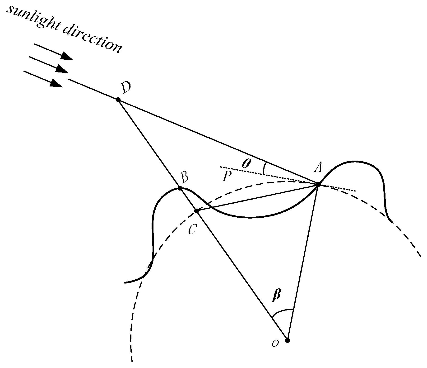
The incident flux in Equation (7) depends on solar illumination. To obtain the flux, we need to know the real-time subsolar point and elevation angle. These parameters are estimated using the SPICE system [24], developed by the NASA Navigation and Ancillary Information Facility (NAIF). The elevation angle is used to determine illumination aspect [192021,35], defined as the angle between the horizon and sunlight direction. As is shown in Figure 2, the dotted line AP signifies the horizon, and the sunlight direction by the line AD. An elevation angle less than zero means the sun is sinking below the horizon at nightfall. In such cases, the boundary conditions for heat conduction in Equation (2) will not include solar flux; however, in the daytime, the elevation angle is required to solve Equation (2).
The effect of terrain obscuration is non-negligible when the elevation angle is considered in the daytime. Such an effect can be determined according to the subsolar point and terrain maps. As shown in Figure 2, the sunlight direction is estimated according to subsolar point. Supposing A denotes the target position on the Moon, we can determine a candidate point B, whether blocking A or not. Figure 2 gives a schematic for the terrain obscuration. The dashed arc denotes an equivalent curved surface with the same radius of point A. B signifies the point used to determine the terrain obscuration, and its projection on the equivalent surface is represented as C. β is the central angle between the points A and B, and its value can be calculated through the two points’ longitudes and latitudes.
The length of line BC can be estimated according to DTM from LOLA. The LOLA team assembled the LOLA data as a global Digital Elevation Model (DEM) in cylindrical and polar stereographic projects. We employed the cylindrical version and applied the LDEM_512_00N_45N_000_090 and LDEM_512_45N_90N_000_090 (1/512° × 1/512°) in our calculations. Supposing sunlight can arrive at point A, the length of line DC needs to be larger than BC. Considering curvature of the lunar surface, we estimated several candidate points along the arc of AC. In practice, a value of β lower than 8 degrees is sufficient to determine the terrain obscuration effect [35]. In the case of sunlight even blocked during the local daytime, we will not consider solar heating in the boundary conditions of Equations (1) and (2).
3. Results and Discussion
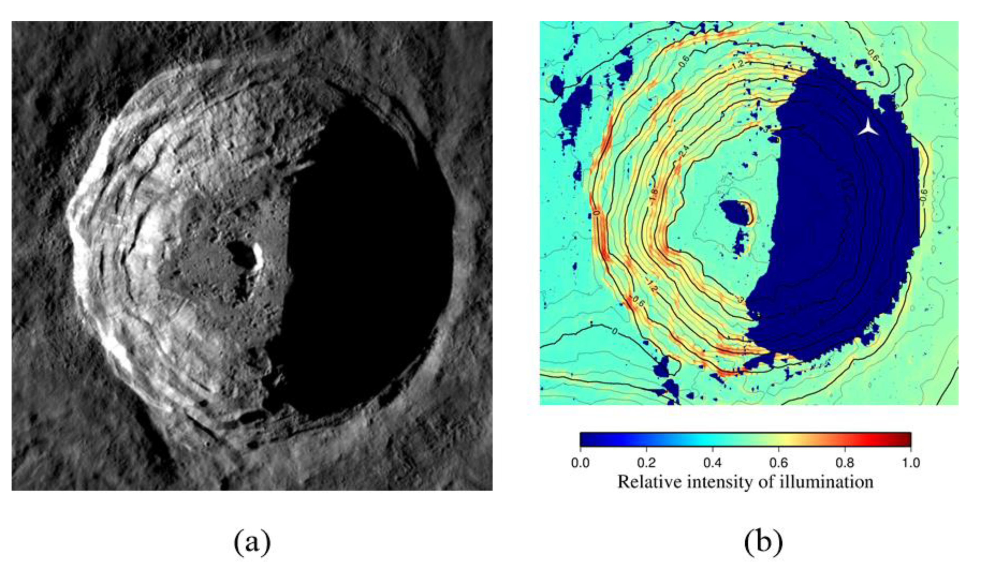
The real-time sunlight direction and elevation angle are estimated with the SPICE system. They are used in our illumination program to test terrain obscuration. To validate this program, Figure 3 gives a comparison between the observed image (Figure 3a) and the synthetic image (Figure 3b) from LOLA.
The illumination aspect is displayed over the Aristarchus crater, centered at (23.73°N, 312.51°E). Figure 3a comes from the narrow-angle camera (NAC) image (http://lroc.sese.asu.edu/posts/291), displaying illumination observed during the morning with the Sun shining from the right. Figure 3b exhibits the corresponding illumination estimated by our program; its contour lines indicate that the minimum elevation of the Aristarchus crater is close to −3.3 km. The color bar demonstrates the range of relative intensity of illumination. The maximum intensity of illumination in Figure 3b arises at the inner wall of Aristarchus crater and is similar to the intensity of illumination in Figure 3a. The shadowed areas in the two figures resemble each other, which mirrors obscuration by terrain features. The resemblance of illumination in the two figures indicates the effectiveness of our program; we employed it to investigate subsurface temperature variation on the Moon.
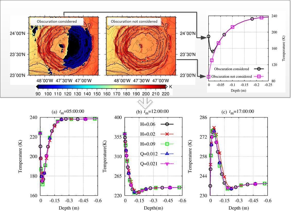
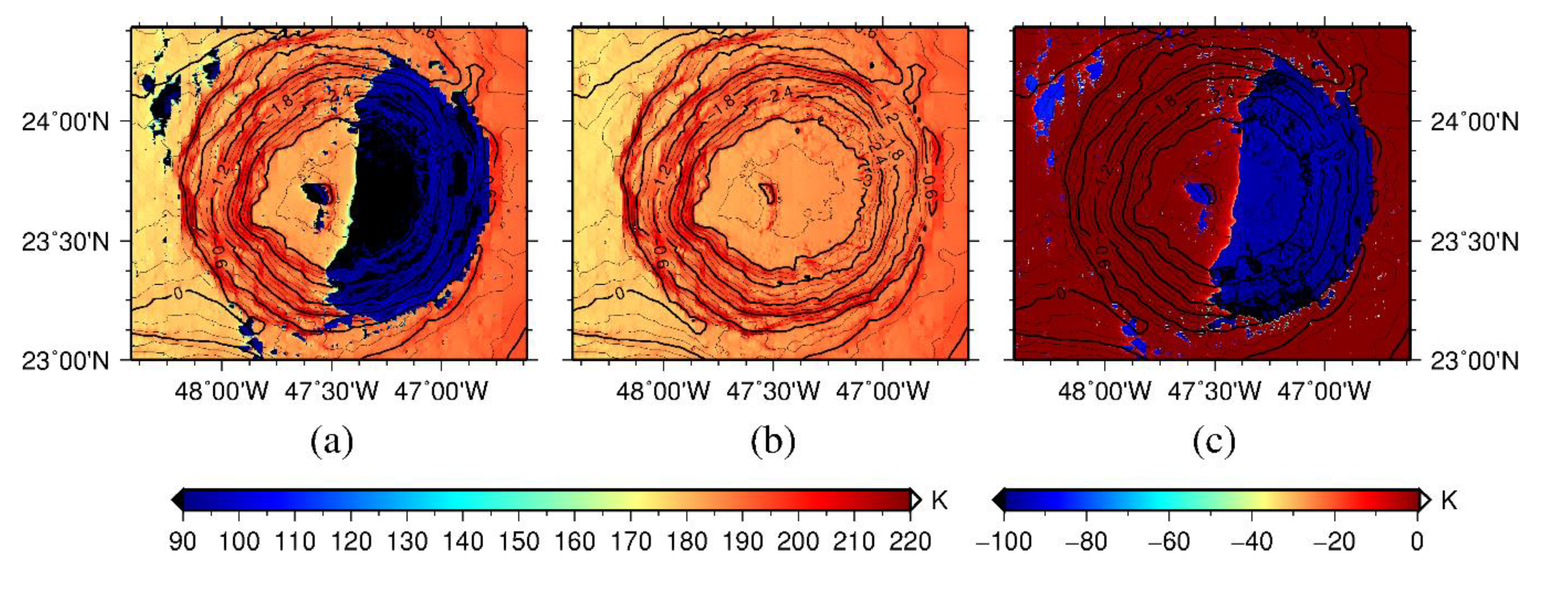
To demonstrate the terrain obscuration affection on temperature, we also studied the surface temperature over Aristarchus with (Figure 4a) and without (Figure 4b) terrain obscuration in Figure 4 at the lunar local time tm = 6:39:31.
Figure 4a,b denotes the surface temperature with and without consideration of terrain obscuration, and Figure 4c represents their temperature residual. Figure 4a indicates that the temperature on the right inner wall is quite cold at 90 K, due to the obscured sunlight, while Figure 4b demonstrates a relatively high temperature to 190 K at the same location. Figure 4c shows the great residual of temperature existing at the right inner wall, where the sunlight is obscured by the surrounding terrain. The right inner wall in Figure 4b is in fact shadowed due to no sunlight arriving; thus, the temperature showing there is unbelievable. It can be concluded that the ignorance of terrain obscuration will lead to untruthful results.
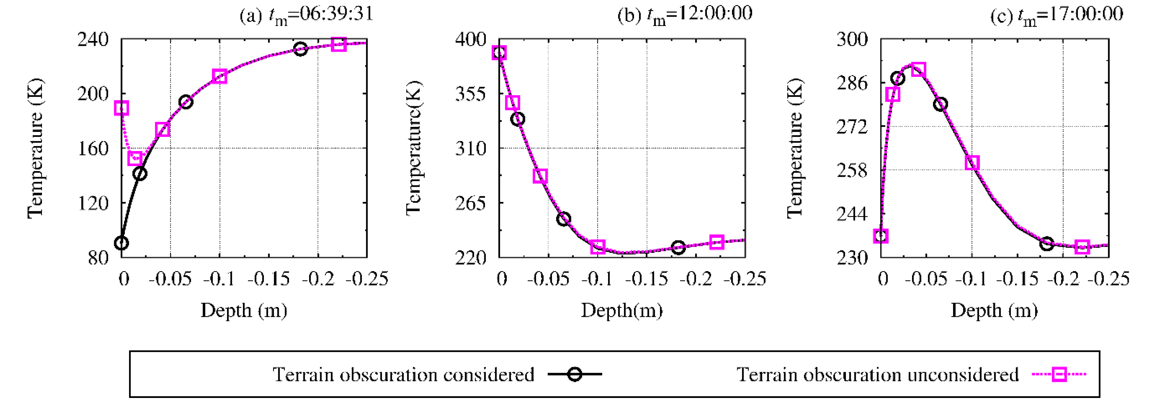
To further explore the temperature variation with depth, Figure 5 gives temperature variation with depth at the point (313°E, 24°N), which is shown in Figure 3 with a sign of white three-star.
Figure 5 denotew profiles of temperature–depth at the lunar local time tm = 06:39:31, tm = 12:00:00, and tm = 17:00:00. The solid black line with circle signifies temperature variation with terrain obscuration, while the dashed pink line with square represents the case without terrain obscuration. Figure 5a indicates that the terrain obscuration affects temperature greatly near to the surface, but the rest of the panels imply that these two cases with and without terrain obscuration have the same performance with the sunlight arriving. It is can be concluded that the terrain obscuration affects the near-surface temperature greatly, but this effect disappears with the depth increased and the sunlight not obscured.
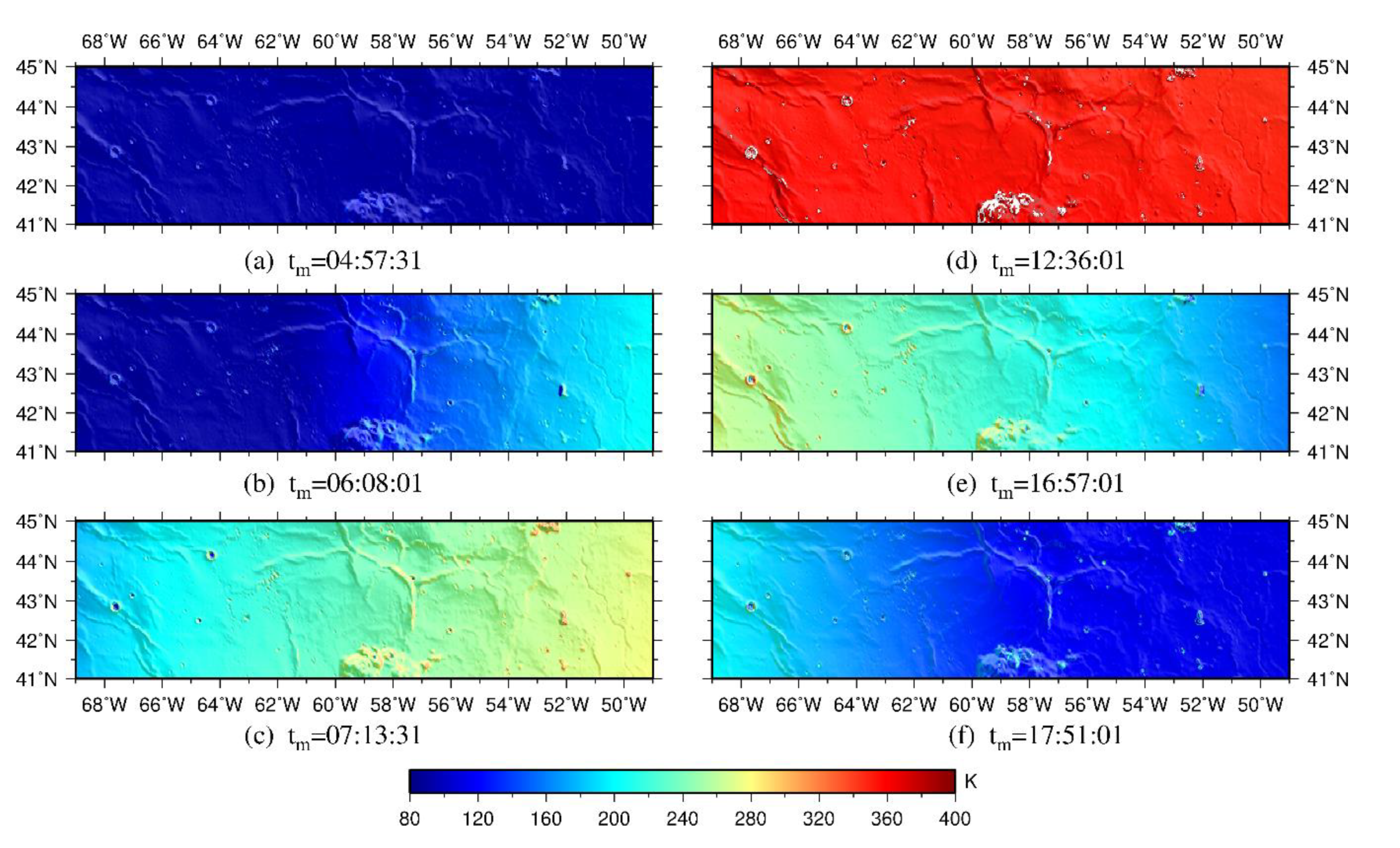
To investigate temperature variation over Rümker region with time, not only a boundary condition, but also an initial condition is needed to solve the heat equation. According to the study [13], an appropriate initial temperature influences temperature variation at depth over time. To reduce errors, we continuously implemented estimation for several lunar days, each one corresponding to about one month on Earth. We selected the most recent lunar day to analyze. In order to take the lunar day associated with UTC on Earth, we took the analyzed lunar days expressed as UTC months. We also supplied the corresponding lunar local time. Although the CE-5 is scheduled to launch in 2020, the exact date of landing implementation is difficult to predict now. Considering previous Chinese lunar exploration projects such as Chang’E 3 (CE−3) and Chang’E 4 (CE−4), we took five months for the project implementation. The errors generated by initial conditions will be reduced by the last month of the mission, so we selected the last month as the research period and analyzed the temperature. The research period will last from UTC 2020-0-3T00:00:01 to 2020-06-01T23:45:01, corresponding to lunar local time from 04:23:01 of the first day to 04:22:31 of the next day. We sampled the days and give the corresponding surface temperature in Figure 6.
The temperature distribution at the time of UTC 2020-0-3T17:15:01 is displayed in Figure 6a, which shows a minimum temperature close to 80 K at night. As the sunlight in Figure 6b arrives in the morning, the temperature increases in the research area at the time of UTC 2020-05-05T04:30:01. As the rising of the Sun, it continues to increase at the time of UTC 2020-06-06T13:15:01 in Figure 6c. At noon, it even climbs to a maximum value of more than 400 K in Figure 6d, corresponding to the time of UTC 2020-05-13T06:30:01. After that, the temperature is declining as the sun is setting, which is exhibited in Figure 6e at the time of UTC 2020-05-18T17:00:01. Finally, the lunar surface becomes quite cold as the sun is sinking behind the horizon. This case is illustrated in Figure 6f, corresponding to the time of UTC 2020-05-19T20:00:01.
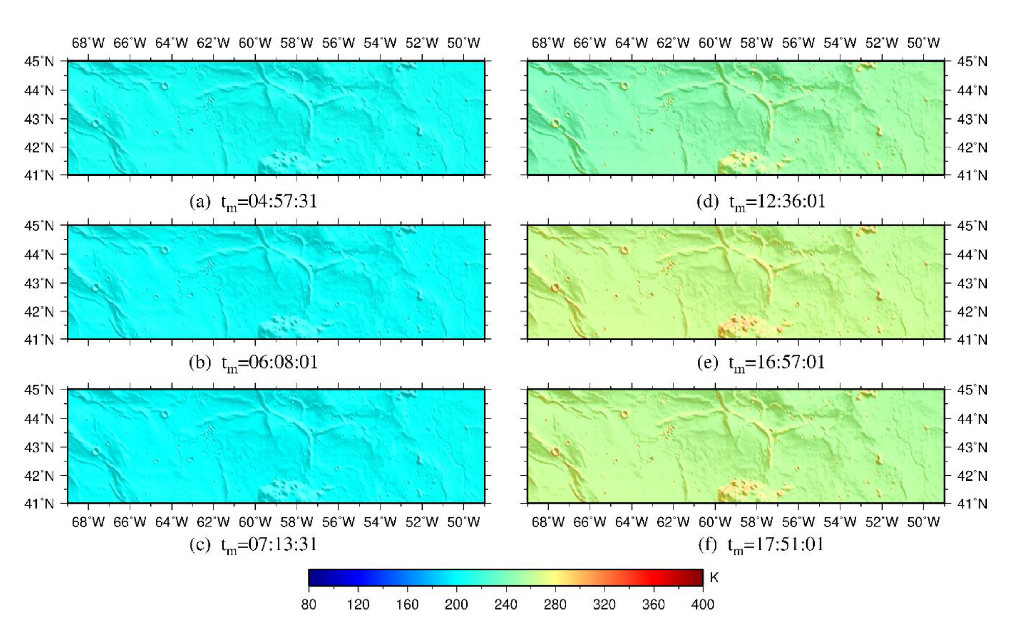
Adopting the same research period, we could analyze subsurface temperature variation. We tested various depths and found that the subsurface temperature does not change at increasing depths. A shallow depth varies from the surface temperature, but at deeper levels, the temperature is nearly constant. After several tests, we found a trade-off depth of 0.0656 m, which demonstrates varying but not significantly different temperatures. This depth illustrates subsurface temperature variation, as shown in Figure 7.
As can be seen from Figure 7a–c, the subsurface temperature changes a little, but remains in a range close to 200 K, unlike the variation seen in Figure 6a–c. The subsurface temperature increases gradually until noon, as shown in Figure 7d. It climbs to a maximum value in Figure 7e, close to 280 K, even when the sun is setting. It does not yet decline greatly in the evening of Figure 5f. This result confirms that the lunar regolith tends to slow down thermal conduction [13,16]. Such thermal insulation could be ascribed to the porous, pulverized, and granular attributes of the regolith, as investigated by the study [23]. Its improvement is the prediction of a lower thermal conductivity but a higher specific heat than previous research [9,10,11,12,13]. Therefore, the subsurface temperature varies more slowly than surface. The differences of temperature variation between Figure 6 and Figure 7 are a mirror of such insulation of lunar regolith.
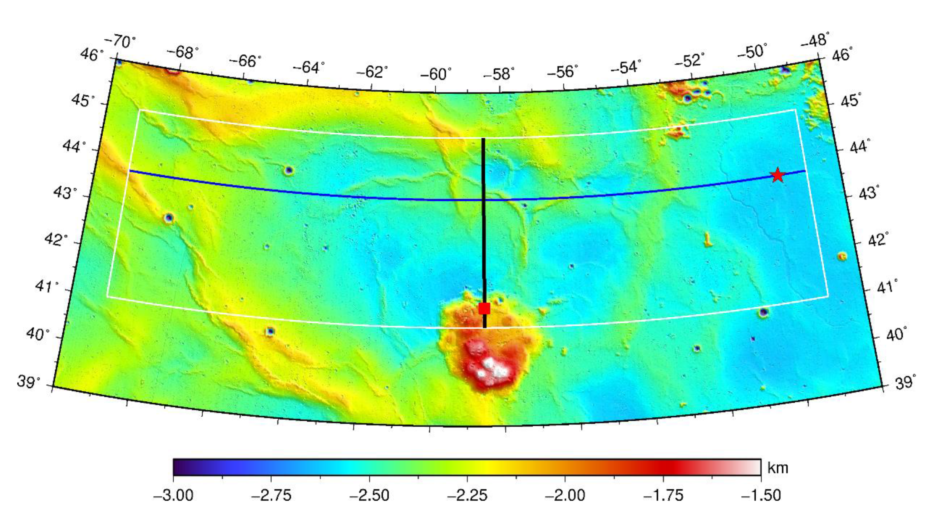
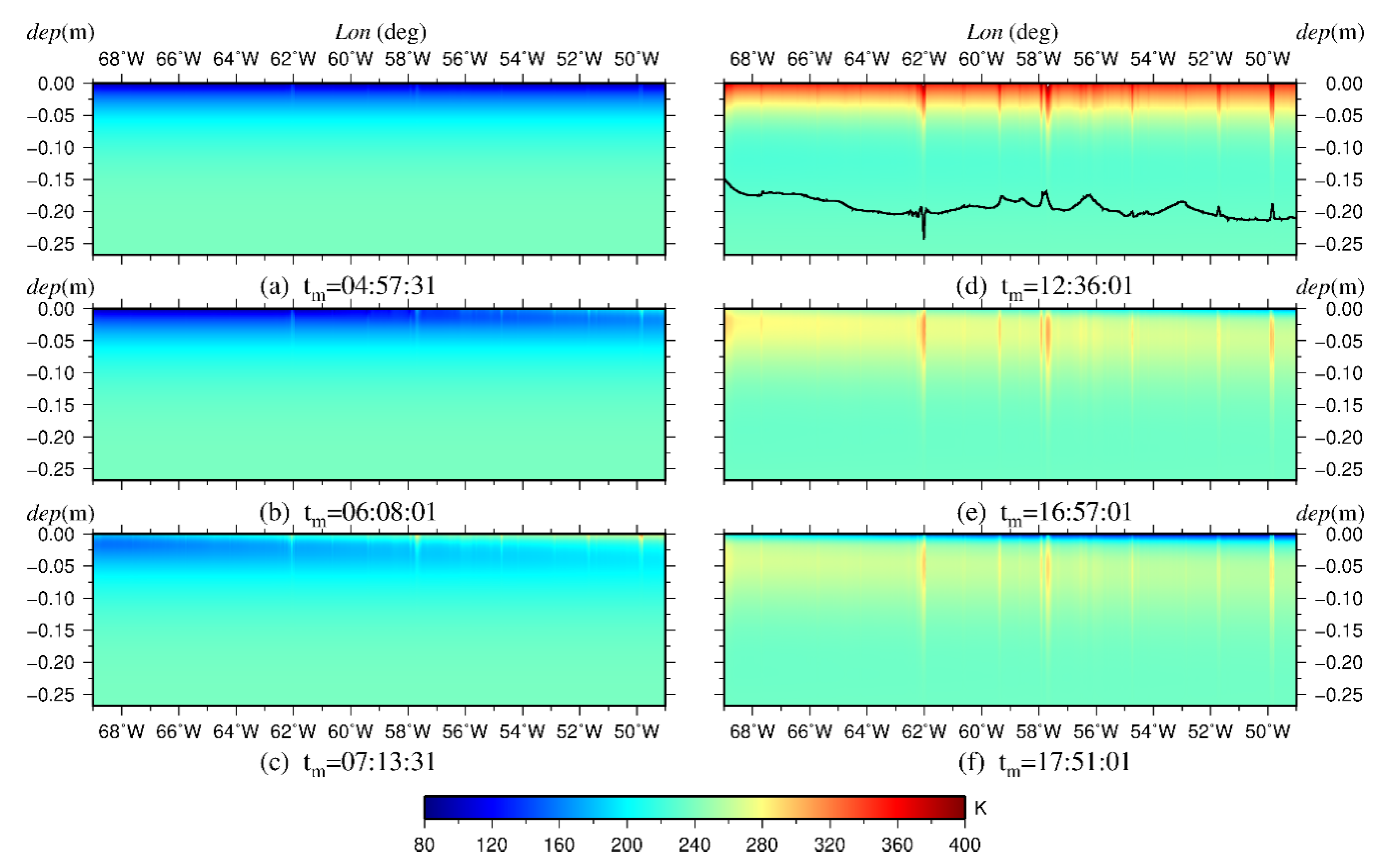
To further probe the subsurface temperature, we investigated the temperature variations in the latitude and longitude directions in Figure 8 and Figure 9, respectively. They all pass through the CE-5 landing sites proposed by the research [2]. These landing sites are indicated with red star and red square, centered at (43.68°N, 49.85°W) and (41.41°N, 58.53°W) in Figure 1. Figure 8 and Figure 9 give temperature variation with time on cross sections and display their results at the same time as those in Figure 6 and Figure 7. Figure 8a–c shows the temperature variation in the longitude direction. The illumination heats the surface layers within 0.05 m as the sun rises. At noon, as seen in Figure 8d, the surface temperature reaches the maximum value, but the subsurface temperature varies little, especially those layers below 0.25 m. After midday, the high temperature at the surface conducts down to the lunar inner layers, which heat up as shown. As the sun sets in Figure 8e,f, the surface temperature declines greatly, but subsurface temperature falls slowly. These results demonstrate the thermal insulation properties of the lunar regolith.
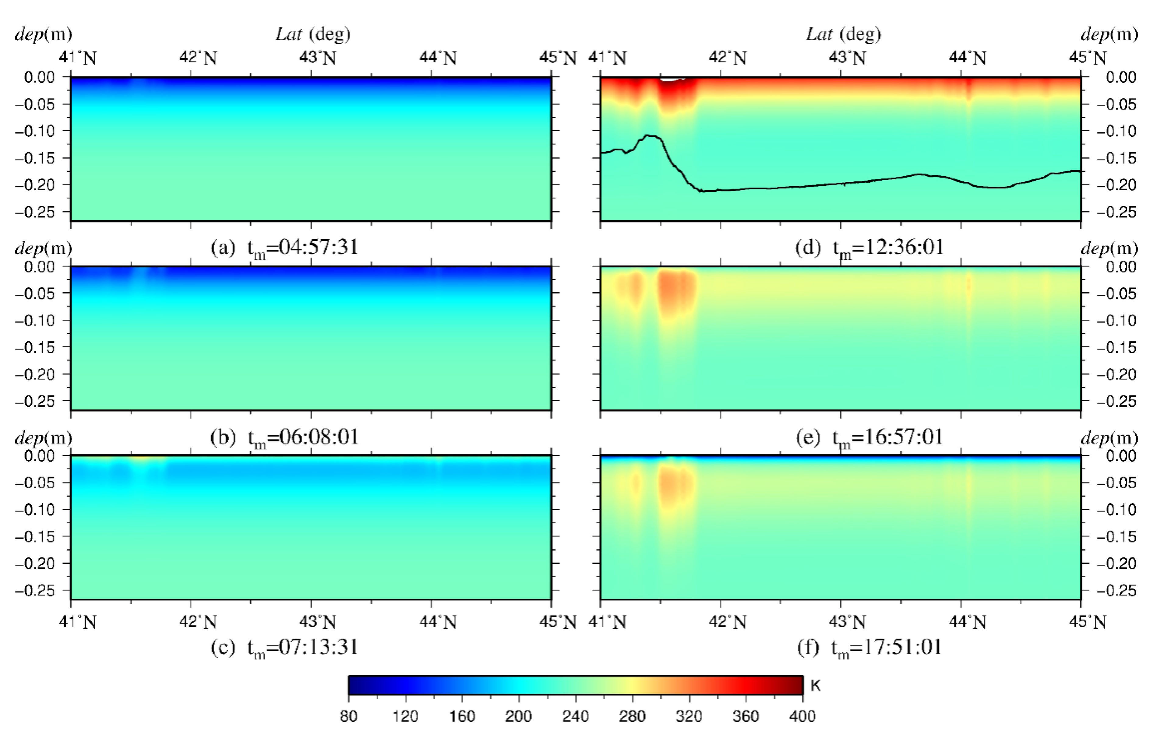
Figure 8a–f shows several stripes of temperature. According to the study [13], a thermal inertia depends on local topographic features. It is used to describe the resistance of materials to changes in temperature. The temperature stripes in Figure 8a–f are a mirror of different topographic features. To display such correlations, Figure 8d gives a black profile line of the surface topography along latitude. This line varies in a range relative to the topography and is not to scale by distance. We also added such a profile of surface topography in Figure 9d in the latitude direction to demonstrate its correlation to the temperature stripes. Such stripes can be found in Figure 9, especially in Figure 9d–f. The stripes with significant variation by depth are on parts of Mons Rümker, which is located on the left part of Figure 9a–f. From the correlation between the topographic terrain and temperature stripes, it could be concluded that the temperature stripes are a mirror of anisotropic thermal inertia. As the sun rises in Figure 9a–c, the surface temperature increases, but inner temperature at layers under 0.25 m changes little. Similarly, in Figure 9d–f, the surface temperature declines gradually, but inner temperature varies slowly, especially those beneath layer of 0.25 m; these results indicate that the lunar regolith has thermal insulation properties. Thus, we provide results within the depth of 0.275 m in Figure 8 and Figure 9, although the temperature estimated ranges within the depth of 2 m.
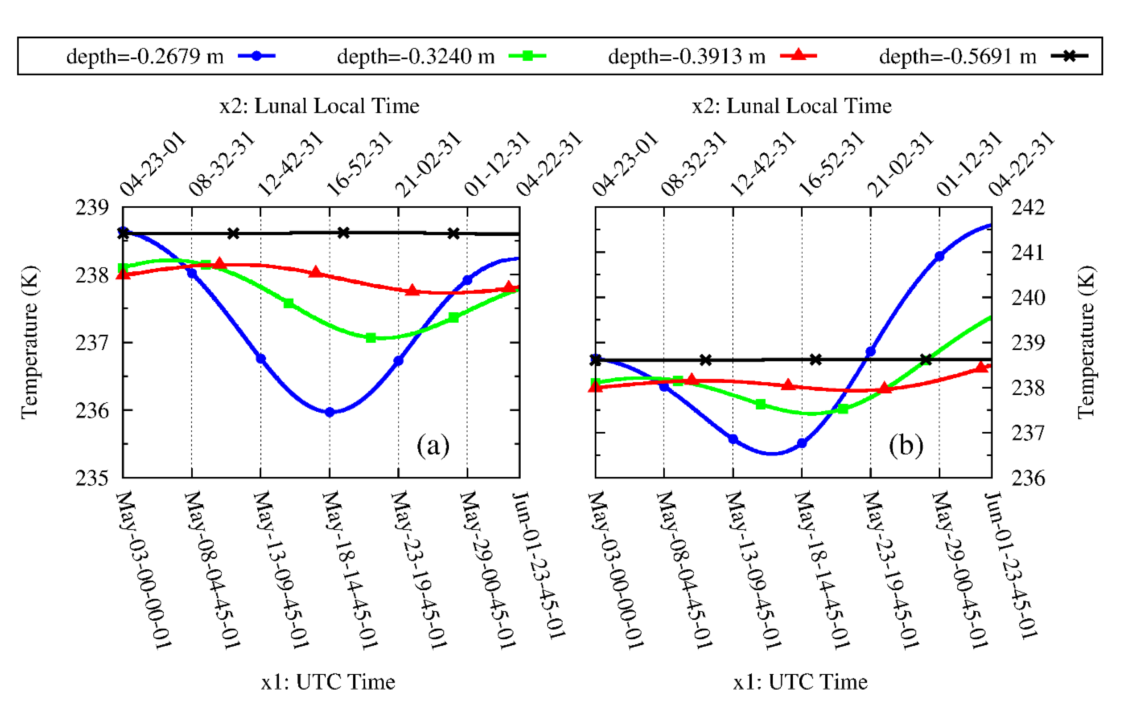
To investigate the subsurface temperature variation beneath 0.25 m further, Figure 10 gives the variations at the proposed two landing sites [2]. As to the point of red square in Figure 1, Figure 10a indicates that the subsurface temperature at −0.2679 m varies between 235.97 K and 238.64 K in the whole research period, but alters a little below this depth. It even keeps in constant at the depth of −0.5691 m. Such constant subsurface temperature, as shown in Figure 10b, is consistent across the other landing sites, marked with a red star in Figure 1. Considering all the results shown in Figure 6, Figure 7, Figure 8, Figure 9 and Figure 10, it can be concluded that the subsurface temperature stays constant under the depth of −0.6 m. As more lunar heat flow measurements needed are to constrain lunar thermal evolution [36], remeasurement at different places is needed in future explorations. Based on the CE-5 drilling experience, China’s next exploration could consider a direct measurement of heat flow, and a drilling depth close to 2 m is adequate to explore the inner heat flow beneath −0.6 m.
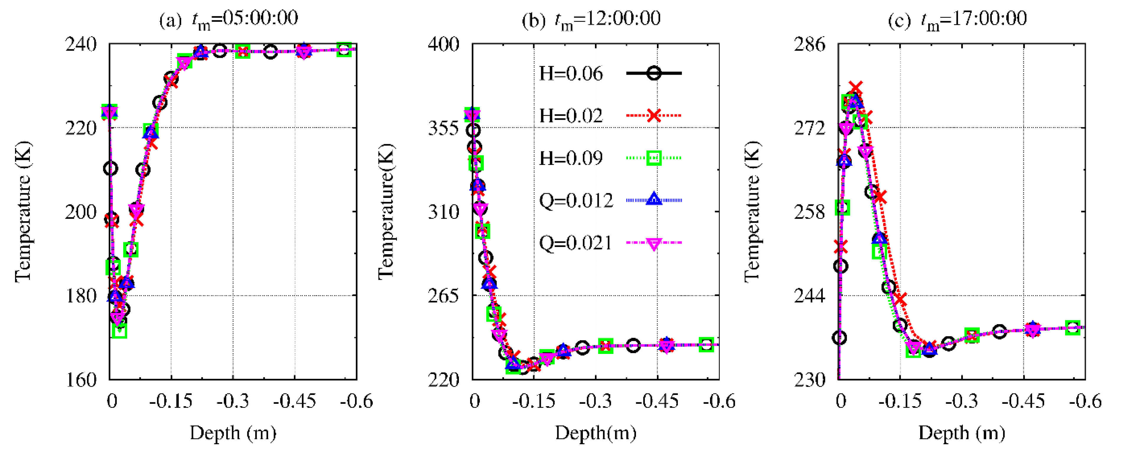
The depth of constant temperature layer found above would depend on H parameter and lunar inner heat flow Q. We next take an analysis of these varied parameters. In the previous study [13], the H parameter ranged from 0.02 m to 0.09 m. In this paper, we used a mean value H = 0.06 m. As to the heat flow [17], the measured heat flow from the Apollo 15 was 21 ± 3 mWm−2, but a low value of 15 ± 2 mWm−2 was found for the Apollo 17. The later studies [37,38] found a global value low to 12 mWm−2. We used a mean value of heat flow Q = 18 mWm−2. As to the layer of constant temperature found above, it is necessary to discuss the uncertainties of the H parameter and heat flow. We here give a profile of temperature−depth for the CE-5 landing site centered at (41.41°N, 58.53°W). The profile is shown in Figure 11, which includes three panels (a–c) representing the lunar local time tm = 05:00:00, tm = 12:00:00, and tm = 17:00:00.
The solid line with circle represents the result for the H parameter equal to 0.06 m, which is the value used in our calculation. The dashed line with the cross denotes the case for H = 0.02 m, while the dashed blue line with square is for H = 0.09 m. The dashed blue line with the upper triangle implies the case with a heat flow low to 12 mWm−2, while the dashed pink line with the lower triangle indicates the case with a large heat flow Q = 21 mWm−2. It can be found that the small and large heat flow changes the profiles little, compared with the mean value Q = 18 mWm−2. The apparent deviation of the profile is mainly contributed by the small H parameter (H = 0.02 m) in the afternoon. However, all the profiles merge with each other with the depth increased, especially low to −0.3 m. This result suggests that the changes of H and Q have no influence on temperature below −0.6 m.
4. Conclusions
In this paper, we studied the lunar regolith temperature variation in the proposed Rümker landing region of CE-5. We investigated the real-time illumination based on the NASA’s SPICE system. Combined with local surface slope and aspect, zenith angle, surface azimuth, and solar azimuth estimations, the real-time solar heating rate was evaluated and used to calculate the relative intensity of illumination in the Aristarchus crater. Our synthetic figure closely resembles the observed NAC image, indicating the effectiveness of our calculations. We also used the real-time solar heating flux to study the temperature variation. The results demonstrate that solar illumination affects the surface temperature, becoming weaker with the increasing depth. In general, the subsurface temperature changes abruptly with the solar illumination around −5 cm. However, temperature anomalies like stripes occur in some places; these can be ascribed to anisotropic thermal inertia. The subsurface temperature fluctuates a little as the depth increases, but remains constant beneath a depth of −0.5691 m. The CE-5 drilling depth will approach 2 m, and thus is adequate to explore the heat flow beneath −0.6 m. This work will be helpful for future Chang’E landing missions to South Polar Region to investigate the subsurface interior temperature variation.
Author Contributions
Conceptualization, Z.Z. and J.Y.; methodology, Z.Z.; software, Z.Z.; validation, Z.Z., J.Y. and Z.X.; formal analysis, Z.Z.; investigation, Z.Z.; resources, Z.Z.; data curation, Z.Z.; writing—original draft preparation, Z.Z.; writing—review and editing, J.Y. and Z.X.; visualization, Z.Z.; supervision, J.Y. and Z.X.; project administration, Z.Z.; funding acquisition, Z.Z. All authors have read and agreed to the published version of the manuscript.
Funding
This research was funded by Grant of National Natural Science Foundation of China (41864001, U1831132, 41773063), Guizhou Science and Technology Plan Project (Guizhou Science and Technology platform talents [2018]5769). Z.X. is supported by the Science and Technology Development Fund of Macau. Grant Number: 0042/2018/A2.
Acknowledgments
The authors would like to thank the scientific team from LRO missions who provide the topography data. These data are downloaded from Planetary Data System website (https://pds.nasa.gov). This research employed the Generic Mapping Tools (GMT) package to produce all the figures.
Conflicts of Interest
The authors declare no conflict of interest.
References
- Zhao, J.; Xiao, L.; Qiao, L.; Glotch, T.D.; Huang, Q. The Mons Rümker volcanic complex of the Moon: A candidate landing site for the Chang’E-5 mission. J. Geophys. Res. Planets 2017, 122, 1419–1442. [Google Scholar] [CrossRef]
- Qian, Y.; Xiao, L.; Zhao, S.Y.; Zhao, J.; Huang, J.; Flahaut, J.; Martinot, M.; Head, J.; Hiesinger, H.; Wang, G.X. Geology and Scientific Significance of the Rümker Region in Northern Oceanus Procellarum: China’s Chang’E-5 Landing Region. J. Geophys. Res. Planets 2018, 123, 1407–1430. [Google Scholar] [CrossRef] [Green Version]
- Chisenga, C.; Yan, J.; Zhao, J.; Atekwana, E.A.; Steffen, R. Density Structure of the Rümker Region in the Northern Oceanus Procellarum: Implications for Lunar Volcanism and Landing Site Selection for the Chang’E-5 Mission. J. Geophys. Res. Planets 2020, 125. [Google Scholar] [CrossRef]
- Yue, Z.; Di, K.; Liu, Z.; Michael, G.; Jia, M.; Xin, X.; Liu, B.; Peng, M.; Liu, J. Lunar regolith thickness deduced from concentric craters in the CE-5 landing area. Icarus 2019, 329, 46–54. [Google Scholar] [CrossRef]
- Zhang, T.; Ding, X. Drilling forces model for lunar regolith exploration and experimental validation. Acta Astronaut. 2017, 131, 190–203. [Google Scholar] [CrossRef]
- Tang, J.; Quan, Q.; Jiang, S.; Liang, J.; Lu, X.; Yuan, F. Investigating the soil removal characteristics of flexible tube coring method for lunar exploration. Adv. Space Res. 2018, 61, 799–810. [Google Scholar] [CrossRef]
- Langseth, M.G.; Keihm, S.J.; Peters, K. Revised lunar heat flow values. In Proceedings of the International Conference on Lunar and Planetary Science, Pergamon, Houston, TX, USA, 15−19 March 1976; pp. 3143–3171. [Google Scholar]
- Mitchell, J.K.; Carrier, W.D., III; Costes, N.C.; Houston, W.N.; Scott, R.F. Surface soil variability and stratigraphy at the Apollo 16 site. In Proceedings of the International Conference on Lunar and Planetary Science, Pergamon, Houston, TX, USA, 5−8 March 1973; pp. 2437–2445. [Google Scholar]
- Paige, D.A.; Siegler, M.A.; Zhang, J.A.; Hayne, P.O.; Foote, E.; Bennett, K.A.; Vasavada, A.R.; Greenhagen, B.T.; Schofield, J.T.; McCleese, D.J.; et al. Diviner lunar radiometer observations of cold traps in the Moon’s south polar region. Science 2010, 330, 479–482. [Google Scholar] [CrossRef] [Green Version]
- Yu, S.; Fa, W. Thermal conductivity of surficial lunar regolith estimated from Lunar Reconnaissance Orbiter Diviner Radiometer data. Planet. Space Sci. 2016, 124, 48–61. [Google Scholar] [CrossRef]
- Williams, J.; Paige, D.; Greenhagen, B.T.; Sefton-Nash, E. The global surface temperatures of the Moon as measured by the Diviner Lunar Radiometer Experiment. Icarus 2017, 283, 300–325. [Google Scholar] [CrossRef] [Green Version]
- Vasavada, A.; Bandfield, J.L.; Greenhagen, B.; Hayne, P.O.; Siegler, M.; Williams, J.; Paige, D.A. Lunar equatorial surface temperatures and regolith properties from the Diviner Lunar Radiometer Experiment. J. Geophys. Res. Space Phys. 2012, 117, 1–12. [Google Scholar] [CrossRef]
- Hayne, P.; Bandfield, J.L.; Siegler, M.A.; Vasavada, A.R.; Ghent, R.R.; Williams, J.; Greenhagen, B.T.; Aharonson, O.; Elder, C.; Lucey, P.G.; et al. Global Regolith Thermophysical Properties of the Moon From the Diviner Lunar Radiometer Experiment. J. Geophys. Res. Planets 2017, 122, 2371–2400. [Google Scholar] [CrossRef] [Green Version]
- Paige, D.A. The thermal stability of near-surface ground ice on Mars. Nature 1992, 356, 43–45. [Google Scholar] [CrossRef]
- Mitchell, D.L.; De Pater, I. Microwave imaging of Mercury’s thermal emission at wavelengths from 0 3 to 20.5 cm. Icarus 1994, 110, 2–32. [Google Scholar]
- Vasavada, A. Near-Surface Temperatures on Mercury and the Moon and the Stability of Polar Ice Deposits. Icarus 1999, 141, 179–193. [Google Scholar] [CrossRef]
- Hayne, P.O.; Greenhagen, B.; Foote, M.C.; Siegler, M.; Vasavada, A.R.; Paige, D.A. Diviner Lunar Radiometer Observations of the LCROSS Impact. Science 2010, 330, 477–479. [Google Scholar] [CrossRef] [PubMed]
- Kieffer, H.H. Thermal model for analysis of Mars infrared mapping. J. Geophys. Res. Planets 2013, 118, 451–470. [Google Scholar] [CrossRef]
- Bussey, B.; Spudis, P.D.; Robinson, M.S. Illumination conditions at the lunar South Pole. Geophys. Res. Lett. 1999, 26, 1187–1190. [Google Scholar] [CrossRef] [Green Version]
- Noda, H.; Araki, H.; Goossens, S.; Ishihara, Y.; Matsumoto, K.; Tazawa, S.; Kawano, N.; Sasaki, S. Illumination conditions at the lunar polar regions by KAGUYA(SELENE) laser altimeter. Geophys. Res. Lett. 2008, 35, 1–5. [Google Scholar] [CrossRef]
- Mazarico, E.; Neumann, G.A.; Smith, D.; Zuber, M.T.; Torrence, M. Illumination conditions of the lunar polar regions using LOLA topography. Icarus 2011, 211, 1066–1081. [Google Scholar] [CrossRef]
- Gläser, P.; Scholten, F.; De Rosa, D.; Figuera, R.M.; Oberst, J.; Mazarico, E.; Neumann, G.A.; Robinson, M. Illumination conditions at the lunar south pole using high resolution Digital Terrain Models from LOLA. Icarus 2014, 243, 78–90. [Google Scholar] [CrossRef]
- Woods-Robinson, R.; Siegler, M.; Paige, D.A. A Model for the Thermophysical Properties of Lunar Regolith at Low Temperatures. J. Geophys. Res. Planets 2019, 124, 1989–2011. [Google Scholar] [CrossRef]
- Acton, C.H., Jr. Ancillary data services of NASA’s Navigation and Ancillary Information Facility, Planet. Space Sci. 1996, 44, 65–70. [Google Scholar] [CrossRef]
- Smith, D.E.; Zuber, M.T.; Neumann, G.A.; Lemoine, F.G.; Mazarico, E.; Torrence, M.H.; McGarry, J.F.; Rowlands, D.D.; Head, J.; Duxbury, T.H.; et al. Initial observations from the Lunar Orbiter Laser Altimeter (LOLA). Geophys. Res. Lett. 2010, 37, 1–6. [Google Scholar] [CrossRef]
- Smith, D.E.; Zuber, M.T.; Neumann, G.A.; Mazarico, E.; Lemoine, F.G.; Iii, J.W.H.; Lucey, P.G.; Aharonson, O.; Robinson, M.S.; Sun, X.; et al. Summary of the results from the lunar orbiter laser altimeter after seven years in lunar orbit. Icarus 2017, 283, 70–91. [Google Scholar] [CrossRef] [Green Version]
- Carrier, W.D.; Olhoeft, G.R.; Mendell, W. Physical properties of the lunar surface. In Lunar Sourcebook; Cambridge University Publishers: Cambridge, UK, 1991; pp. 475–594. ISBN 0-521-33444-6. [Google Scholar]
- Whipple, F.L. A comet model. I. The acceleration of Comet Encke. Astrophys. J. 1950, 111, 375–394. [Google Scholar] [CrossRef]
- Fountain, J.A.; West, E.A. Thermal conductivity of particulate basalt as a function of density in simulated lunar and Martian environments. J. Geophys. Res. Space Phys. 1970, 75, 4063–4069. [Google Scholar] [CrossRef]
- Ledlow, M.J.; Zeilik, M.; Burns, J.O.; Gisler, G.R.; Zhao, J.H.; Baker, D.N. Subsurface emissions from Mercury-VLA radio observations at 2 and 6 centimeters. Astrophys. J. 1992, 384, 640–655. [Google Scholar] [CrossRef]
- Hemingway, B.S.; Krupka, K.M.; Robie, R.A. Heat capacities of the alkali feldspars between 350 and 1000 K from differential scanning calorimetry, the thermodynamic functions of the alkali feldspars from 298.15 to 1400 K, and the reaction quartz + jadeite = analbite. Am. Mineral. 1981, 66, 1202–1215. [Google Scholar]
- Keihm, S.J. Interpretation of the lunar microwave brightness temperature spectrum: Feasibility of orbital heat flow mapping. Icarus 1984, 60, 568–589. [Google Scholar] [CrossRef]
- Kopp, G.; Lean, J.L. A new, lower value of total solar irradiance: Evidence and climate significance. Geophys. Res. Lett. 2011, 38, 541–551. [Google Scholar] [CrossRef] [Green Version]
- Braun, J.; Mitchell, J. Solar geometry for fixed and tracking surfaces. Sol. Energy 1983, 31, 439–444. [Google Scholar] [CrossRef]
- Hao, W.; Zhu, C.; Li, F.; Yan, J.; Ye, M.; Barriot, J.P. Illumination and communication conditions at the Mons Rümker region based on the improved Lunar Orbiter Laser Altimeter data. Planet. Space Sci. 2019, 168, 73–82. [Google Scholar] [CrossRef]
- Siegler, M.A.; Smrekar, S.E. Lunar heat flow: Regional prospective of the Apollo landing sites. J. Geophys. Res. Planets 2014, 119, 47–63. [Google Scholar] [CrossRef]
- Rasmussen, K.L.; Warren, P.H. Megaregolith thickness, heat flow, and the bulk composition of the Moon. Nature 1985, 313, 121–124. [Google Scholar] [CrossRef]
- Warren, P.H.; Rasmussen, K.L. Megaregolith insulation, internal temperatures, and bulk uranium content of the moon. J. Geophys. Res. Space Phys. 1987, 92, 3453–3465. [Google Scholar] [CrossRef]
Figure 1.
Elevation map of Rümker region, which is plotted with Lambert conformal conic projection. The elevation data comes from Lunar Orbiter Laser Altimeter (LOLA) Digital Elevation Model (DEM) models of LDEM_512_00N_45N_000_090.IMG, and LDEM_512_45N_90N_000_090.IMG. The white box signifies the candidate landing region of CE-5. The red star denotes the candidate landing site centered at (43.68°N, 49.85°W), the red box signifies the possible landing site centered at (41.41°N, 58.53°W). The blue and black lines are the longitude and latitude directions used to investigate temperature variation in Figure 8 and Figure 9, respectively.

Figure 2.
Schematic of illumination condition.

Figure 3.
Comparison of illumination condition over Aristarchus crater. (a) comes from the narrow-angle camera (NAC) image (http://lroc.sese.asu.edu/posts/291) with a subsolar point longitude 34.0°E and (b) is computed from our illumination program. It is noted that minor differences caused by the limited resolution of digital elevation model exists between the observed (a) and modeled illumination distribution (b). The white three-star denotes the point (313°E, 24°N) used to test terrain obscuration at three lunar local time.

Figure 4.
The surface temperature over Aritarchus with (a) and without (b) terrain obscuration, and their residual (c) at the lunar local time tm = 6:39:31.
Figure 4.
The surface temperature over Aritarchus with (a) and without (b) terrain obscuration, and their residual (c) at the lunar local time tm = 6:39:31.

Figure 5.
Profile of temperature–depth with (solid black line with circle) and without (dashed pink line with square) terrain obscuration. The panels (a) and (b) denote profiles at the lunar time tm = 06:39:31 and tm = 12:00:00, respectively, and (c) represents that at tm = 17:00:00.
Figure 5.
Profile of temperature–depth with (solid black line with circle) and without (dashed pink line with square) terrain obscuration. The panels (a) and (b) denote profiles at the lunar time tm = 06:39:31 and tm = 12:00:00, respectively, and (c) represents that at tm = 17:00:00.

Figure 6.
Surface temperature variation with different time. (a) Universal Time Coordinated (UTC) 2020-05-03T17:15:01; (b) UTC 2020-05-05T04:30:01; (c) UTC 2020-05-06T13:15:01; (d) UTC 2020-05-13T06:30:01; (e) UTC 2020-05-18T17:00:01; (f) UTC 2020-05-19T20:00:01. tm represents the lunar local time.
Figure 6.
Surface temperature variation with different time. (a) Universal Time Coordinated (UTC) 2020-05-03T17:15:01; (b) UTC 2020-05-05T04:30:01; (c) UTC 2020-05-06T13:15:01; (d) UTC 2020-05-13T06:30:01; (e) UTC 2020-05-18T17:00:01; (f) UTC 2020-05-19T20:00:01. tm represents the lunar local time.

Figure 7.
Subsurface temperature variation with different time at the depth of −0.0656 m. (a) UTC 2020-0-3T17:15:01; (b) UTC 2020-05-05T04:30:01; (c) UTC 2020-05-06T13:15:01; (d) UTC 2020-05-13T06:30:01; (e) UTC 2020-05-18T17:00:01; (f) UTC 2020-05-19T20:00:01. tm represents the lunar local time.
Figure 7.
Subsurface temperature variation with different time at the depth of −0.0656 m. (a) UTC 2020-0-3T17:15:01; (b) UTC 2020-05-05T04:30:01; (c) UTC 2020-05-06T13:15:01; (d) UTC 2020-05-13T06:30:01; (e) UTC 2020-05-18T17:00:01; (f) UTC 2020-05-19T20:00:01. tm represents the lunar local time.

Figure 8.
Temperature variation along the latitude direction. (a) UTC 2020-0-3T17:15:01; (b) UTC 2020-05-05T04:30:01; (c) UTC 2020-05-06T13:15:01; (d) UTC 2020-05-13T06:30:01; (e) UTC 2020-05-18T17:00:01; (f) UTC 2020-05-19T20:00:01. The black line in Figure 8d denotes the surface topography with fixed latitude 43.68°N but varied longitude. tm represents the lunar local time.

Figure 9.
Temperature variation along the latitude direction. (a) UTC 2020-0-3T17:15:01; (b) UTC 2020-05-05T04:30:01; (c) UTC 2020-05-06T13:15:01; (d) UTC 2020-05-13T06:30:01; (e) UTC 2020-05-18T17:00:01; (f) UTC 2020-05-19T20:00:01. The black line in Figure 9d denotes the surface topography with fixed longitude 58.53°W but varied latitude. tm represents the lunar local time.

Figure 10.
Subsurface temperature variations at the two landing sites [2]. (a) denotes variations for the red square points, and (b) represents those for the red star in Figure 1. The border-down x1 represents UTC time, while the border-up x2 denotes lunar local time.

Figure 11.
Profiles of temperature–depth for the CE-5 candidate landing site centering at (41.41°N, 58.53°W). The panels (a–c) represent results at the lunar local time tm = 05:00:00, tm = 12:00:00, and tm = 17:00:00.
Figure 11.
Profiles of temperature–depth for the CE-5 candidate landing site centering at (41.41°N, 58.53°W). The panels (a–c) represent results at the lunar local time tm = 05:00:00, tm = 12:00:00, and tm = 17:00:00.

© 2020 by the authors. Licensee MDPI, Basel, Switzerland. This article is an open access article distributed under the terms and conditions of the Creative Commons Attribution (CC BY) license (http://creativecommons.org/licenses/by/4.0/).
Share and Cite
MDPI and ACS Style
Zhong, Z.; Yan, J.; Xiao, Z. Lunar Regolith Temperature Variation in the Rümker Region Based on the Real-Time Illumination. Remote Sens. 2020, 12, 731. https://0-doi-org.brum.beds.ac.uk/10.3390/rs12040731
AMA Style
Zhong Z, Yan J, Xiao Z. Lunar Regolith Temperature Variation in the Rümker Region Based on the Real-Time Illumination. Remote Sensing. 2020; 12(4):731. https://0-doi-org.brum.beds.ac.uk/10.3390/rs12040731
Chicago/Turabian StyleZhong, Zhen, Jianguo Yan, and Zhiyong Xiao. 2020. "Lunar Regolith Temperature Variation in the Rümker Region Based on the Real-Time Illumination" Remote Sensing 12, no. 4: 731. https://0-doi-org.brum.beds.ac.uk/10.3390/rs12040731
Note that from the first issue of 2016, this journal uses article numbers instead of page numbers. See further details here.