Characteristics Analysis of Raw Multi-GNSS Measurement from Xiaomi Mi 8 and Positioning Performance Improvement with L5/E5 Frequency in an Urban Environment

Abstract

Achieving continuous and high-precision positioning services via smartphone under a Global Navigation Satellite System (GNSS)-degraded environment is urgently demanded by the mass market. In 2018, Xiaomi launched the world’s first dual-frequency GNSS smartphone, Xiaomi Mi 8. The newly added L5/E5 signals are more precise and less prone to distortions from multipath reflections. This paper discusses the characteristics of raw dual-frequency GNSS observations from Xiaomi Mi 8 in urban environments; they are characterized by high pseudorange noise and frequent signal interruption. The traditional dual-frequency ionosphere-free combination is not suitable for Xiaomi Mi 8 raw GNSS data processing, since the noise of the combined measurements is much larger than the influence of the ionospheric delay. Therefore, in order to reasonably utilize the high precision carrier phase observations, a time differenced positioning filter is presented in this paper to deliver continuous and smooth navigation results in urban environments. The filter first estimates the inter-epoch position variation (IEPV) with time differenced uncombined L1/E1 and L5/E5 carrier phase observations and constructs the state equation with IEPV to accurately describe the user’s movement. Secondly, the observation equations are formed with uncombined L1/E1 and L5/E5 pseudorange observations. Then, kinematic experiments in open-sky and GNSS-degraded environments are carried out, and the proposed filter is assessed in terms of the positioning accuracy and solution availability. The result in an open-sky environment shows that, assisted with L5/E5 observations, the root mean square (RMS) of the stand-alone horizontal and vertical positioning errors are about 1.22 m and 1.94 m, respectively, with a 97.8% navigation availability. Encouragingly, even in a GNSS-degraded environment, smooth navigation services with accuracies of 1.61 m and 2.16 m in the horizontal and vertical directions are obtained by using multi-GNSS and L5/E5 observations.

1. Introduction

According to the Global Navigation Satellite System (GNSS) Market 2017 Report, about 6.4 billion smartphones embedded with GNSS chipsets will be active worldwide by 2020 [1]. Various location-based services (LBSs) are essential in mobile applications [2,3], such as turn-by-turn navigation, infotainment, and social networking applications which require GNSS positioning accuracy of about 5 m [1]. Moreover, in recent years, a burgeoning group of new applications has emerged within smartphones that require far more accuracy positioning results, such as augmented reality, seamless image-based navigation, and a smartphone-based photogrammetric unmanned aerial vehicle (UAV) system [4,5,6]. All these applications inspire the development of accurate and continuous navigation solutions based on smartphones. Prior to 2016, the GNSS chipsets in smartphones only outputted the position-velocity-time and limited satellite information such as the elevation and azimuth [7]. The positioning accuracy only reached 2–3 m, and even degraded to 10 m or worse in the case of adverse multipath conditions [8].

The revolution started in May 2016 when Google announced that raw GNSS measurements will be available to the public through the Android Nougat operating system (Android N). Subsequently, many studies attempted to refine the smartphone raw measurement error model and develop advanced algorithms to improve positioning accuracy. In the beginning, mainstream portable smart devices were only embedded with L1/E1 single-frequency GNSS chipsets. The quality assessments of raw GNSS measurements from smartphones showed that the C/N0 of smartphones was about 10 dBHz lower than geodetic receivers [2], and the noise of the L1/E1 pseudorange observation was about 10 times larger than that of a geodetic-quality receiver [9]. The quality analysis for the carrier phase measurements demonstrated that the noise of carrier phase observation was about 0.1 cycle [9], which might have the potential to provide decimeter-level or better positioning accuracy [10]. As a response to these expectations, high-precision GNSS positioning attempts were conducted on Android N. For example, a series of conventional real-time kinematic (RTK) tests were conducted with static and dynamic raw measurements under open environments, and a decimeter-level positioning accuracy was achieved [9,11,12]. As for the positioning performance under complex dynamic environments, Zhang et al. adopted a time-differenced filtering to process the raw Global Positioning System (GPS) L1 measurements from a Nexus 9 tablet in the GNSS-degraded environment, and the resulting position trajectory fluctuated seriously and obvious discontinuities existed [2]. Clearly, due to low-cost single frequency GNSS chipsets and linearly polarized planar inverted F (PIF) antenna embedded in smartphones, the quality of the raw single frequency GNSS observations is usually poor [13,14]. The navigation performance is thus unsatisfactory especially in GNSS-degraded environments.

Innovatively, in 2018, the world’s first dual-frequency GNSS smartphone, Xiaomi Mi 8, fitted with Broadcom’s BCM47755 chipset, was released [15,16]. The newly added L5/E5 signals with binary phase-shift keying (BPSK(10)) and alternative binary offset carrier (AltBOC(15,10)) modulation were superior, especially in cities, where they are less prone to distortions from multipath reflections than L1/E1 [17,18]. The quality assessments for static Xiaomi Mi 8 GNSS measurements showed that characteristics of the C/N0 and carrier phase noise are similar to that of previous single frequency smartphones [19]. The L1/E1 pseudorange observation noise was about 4~7 m for most GNSS observations, but the noise of L5/E5 pseudorange observations was only about 1.5 m. Moreover, the L5/E5 signals have a lower pseudorange multipath error [20]. The better quality of the L5/E5 measurements may be a key to improving the navigation performance of smartphones. Subsequently, a series of high precise positioning algorithms based on the raw Xiaomi Mi 8 GNSS observations were carried out. Conventional dual-frequency (ionosphere-free combination of pseudorange and carrier phase) and single-frequency precise point positioning (PPP) with raw GPS + Galileo observations from Xiaomi Mi 8 showed that, in the static open environment, decimeter-level positioning accuracy was obtained after about 102 min. In the kinematic tests, the positioning tracks had severe fluctuations of approximately 3~5 m with respect to the reference solutions [21,22]. Surprisingly, the single-frequency PPP provided a better solution than the dual-frequency one [16,21]. After analyzing the characteristic of raw pseudorange and carrier phase observations, a modified PPP strategy was proposed by estimating separate clock biases for pseudorange and carrier phase observations [23]. The static PPP experiments with raw GPS, BeiDou, and Galileo data from Xiaomi Mi 8 under an open environment showed that the positioning errors in the north and east directions would converge to within 1 m in 30 s [23]. When conducting RTK with raw GPS, Galileo, and GLObal NAvigation Satellite System (GLONASS) observations from Xiaomi Mi 8 under complex dynamic environments, the horizontal accuracy of 1.17 m was obtained but the solution tracks were still severely fluctuated [16]. To sum up, previous positioning experiments with raw GNSS measurements under open static environments could achieved decimeter-level positioning accuracy. Yet in complex urban environments, since buildings and trees have severe occlusion to GNSS signals, the frequent signal interruptions and ambiguity re-initialization cause degradation of the availability of the PPP and RTK; additionally, the positioning trajectories are unsmooth and have severe fluctuations. In addition, even though Xiaomi Mi 8 outputs dual-frequency measurements, traditional ionosphere-free combination may not always provide the best solution. Therefore, further researches on how to achieve continuous and smooth results in complex urban environments based on the raw smartphone GNSS measurements and how to make full use of the high-quality L5/E5 measurements to improve navigation accuracy are needed.

In this paper, we focus on the standalone smartphone navigation problem in GNSS-degraded environments. We assume only the broadcast ephemeris is available, and there are no communications to obtain measurement data from reference stations or the State Space Representation (SSR) product from analysis centers. We use the Xiaomi Mi 8 smartphone as the navigation tool. As such, the characteristic of raw multi-GNSS observations from Xiaomi Mi 8 under static open and dynamic complex environments is assessed in terms of not only C/N0, noise of pseudorange, and carrier phase observations, but also the approximate percentage of pseudorange gross errors and carrier phase cycle slips. Then, considering the frequent signal interruptions and carrier phase cycle slips of raw Xiaomi Mi 8 observations under a complex navigation environment, an improved time-differenced navigation algorithm using raw dual-frequency multi-GNSS measurements from the smartphone is proposed. In particular, the method of properly using high-quality L5/E5 observations is discussed. Dedicated experiments under static-open and dynamic GNSS-degraded environments are carried out to verify the effectiveness of the algorithm and analyze the possibility of using raw GNSS from Xiaomi Mi 8 to achieve meter level continuous and smooth navigation in an urban environment.

The rest of this paper is organized as follows. Section 2 describes the experimental data collection under static open-sky and dynamic GNSS-degraded environments. In Section 3, the characteristics of raw dual-frequency and multi-GNSS observations of Xiaomi Mi 8 in terms of not only C/N0, pseudorange, and carrier phase errors, but also the percentage of pseudorange gross errors and carrier phase cycle slips are discussed. A time differenced filter algorithm is proposed in Section 4 to improve the positioning performance with raw GNSS data from Xiaomi Mi 8. In Section 5, dedicated experiments under different observation environments are conducted to evaluate the proposed algorithm in terms of the positioning accuracy and navigation availability. Finally, some conclusions are given in Section 6.

2. Data Collection

In order to comprehensively understand the characteristics of raw GNSS observations from Xiaomi Mi 8 and assess its navigation performance under different environments, static and kinematic experiments were carried out. It should be noted that, during GNSS data collection, the Wi-Fi and Bluetooth of Xiaomi Mi 8 were turned off to avoid disturbances from these sensors, and only the location permission was accessed. The system of the Xiaomi Mi 8 smartphone used in the experiments was Android 8.0, whose battery saving mechanism for the GNSS chip, ‘duty cycle’, was off by default.

2.1. Static GNSS Data Collection

The static smartphone raw GNSS data acquisition was made on the roof of Wuhan University School of Geodesy and Geomatics building, with the antennas setting depicted in Figure 1. One geodetic-quality Trimble Zephyr Geodetic Model 2 antenna connecting to a Septentrio PolaRx5 receiver was used as a reference station. A NovAtel GPS-704-WB antenna connecting to a Septentrio PolaRx5s receiver, mounted on the other measuring pillar, was used as a rover station. The distance between the two geodetic-quality antennas was less than 5 m. An android smartphone Xiaomi Mi 8 was located next to the NovAtel GPS-704-WB antenna on the measuring pillar. After the Xiaomi Mi 8 data collection, a microstrip antenna connected to a u-blox M8T receiver was placed at the same spot occupied by the Xiaomi Mi 8, in order to obtain the precise position of the Xiaomi Mi 8 by RTK with the base station. The raw Android GNSS observations were collected on 24 January 2019 with a data rate of 1 Hz for approximately 8 h through the GNSSLogger App released by Google [10]. The observed L1/E1 and L5/E5 sky plots and availability of some of the satellites for Xiaomi Mi 8 are shown in Figure 2, plotted by RTKLIB [24]. The short red line is the AccumulatedDeltaRangeState (ADRS) field provided by Android smartphone, which indicates the validity of the carrier measurement. Cycle slips are reflected in the ADRS [25]. It is seen that about 25 satellites were viewed on L1/E1 frequency and 11 satellites on L5/E5 frequency. In addition, for this static data, most carrier phase cycle slips occur at low satellite elevation, and the cycle slips may not appear on L1/E1 and L5/E5 simultaneously, such as satellites J03.

2.2. Dynamic GNSS Data Collection

The purpose of the dynamic test is to analyze the characteristics of raw observations in dynamic GNSS-degraded environments and the navigation performance improvement by the use of multi-GNSS and dual-frequency observations. Two predesigned tracks, as shown in Figure 3, were used: track 1 was mostly under an open sky on the playground (red dots) and track 2 was on a road surrounded by dense trees and buildings (white dots), where the GNSS signal was significantly degraded. The test devices are illustrated in Figure 4. A utility cart carrying NovAtel’s SPAN GNSS Inertial Navigation System and Xiaomi Mi 8 was used to perform the dynamic test. The NovAtel’s SPAN GNSS Inertial Navigation System used in our experiments was an earlier version of the device, which supports GPS and GLONASS. Another reference station, whose coordinates were known, was the choke-ring antenna connected to a NovAtel ProPak 6 on the roof of Wuhan University School of Geodesy building. The distance between the reference station and the utility cart was less than 500 m during the experiment. In track 1, the NovAtel software Inertial Explorer (IE) was used to analyze the SPAN system data by RTK and inertial navigation system (INS) combination and then a reference trajectory was obtained. Considering the distance between the phase center of SPAN GNSS antenna and the Xiaomi Mi 8 smartphone, an arm correction was applied to reduce the reference trajectory to the position of Xiaomi Mi 8. In the GNSS-degraded environment of track 2, GPS signal interruption was serious, and no reliable reference trajectory was available. Alternatively, several reference points on the route, shown as orange points in Figure 3, whose precise coordinates were determined by post double-frequency RTK or surveyed using total station, were used to evaluate positioning accuracy. The Android raw GNSS observations were collected on 18 December 2018 with 1-s sampling interval for approximately 2 h. The cart speed was about 1.0 m/s. The observed L1/E1 and L5/E5 sky plots and availability of parts of the satellites for Xiaomi Mi 8 are shown in Figure 5. Clearly, the characteristic of ADRS is quite different from that in Figure 2. In the dynamic situation, more frequent carrier phase cycle slips exist, and there is no obvious correlation between cycle slips and satellite elevation.

3. Characteristics of Xiaomi Mi 8 Raw GNSS Observations

If a low-cost linearly polarized PIF antenna is embedded in Xiaomi Mi 8, it will lead to lower antenna gain and lower C/N0 value, making Xiaomi Mi 8 more sensitive to multipath interference and resulting in more gross errors in observations. In the following sections, we analyze the signal strength and error characteristics of the raw GNSS observations from Xiaomi Mi 8, and explore the approximate percentage of pseudorange gross errors and carrier phase cycle slips, especially in GNSS-degraded environments. These analyses support the subsequent design of the high-precision pedestrian navigation algorithm.

3.1. Carrier-to-Noise Density Ratio

The C/N0 measured by the receiver is a diagnostic of both the signal power of tracked satellite and the noise density of the front-end [26,27]. A larger C/N0 indicates a stronger signal and a better observation quality for positioning; a lower C/N0 usually implicates a high probability of outliers and cycle slips.

Figure 6 and Figure 7 show normalized histograms, displaying the drop in C/N0 value between the survey-grade receiver Septentrio PolaRx5, and Xiaomi Mi 8 for GPS (G), GLONASS (R), Galileo (E), BeiDou (C), and Quasi-Zenith Satellite System (QZSS) (J) on frequency L1/E1 and L5/E5, of the tracked satellites ranging in elevation from 15 to 90 degrees. The Septentrio PolaRx5s connecting to a survey-grade antenna, which has a uniform quasi-hemispherical gain pattern, right-hand circular polarization, and a stable phase center, only has a ±1.0 dBHz fluctuation in its C/N0 value on average relative to the reference station receiver. However, as for the linear polarization antenna embedded in Xiaomi Mi 8, the C/N0 reductions compared to the survey-grade antenna vary with respect to different navigation satellite systems and different frequencies. The average C/N0 drop is about 6, 10, 9, 11, and 7 dBHz for L1/E1 observations of the GPS, GLONASS, Galileo, BeiDou, and QZSS satellites, respectively; while the C/N0 drop in the normalized histograms for L5/E5 observations is quite different from that of L1/E1, with the main reduction from 5 to 15 dBHz and remaining relatively flat. This may be due to the imperfect antenna design of Xiaomi Mi 8 for capturing multi-frequency signals.

In order to further analyze the characteristic of C/N0 against the elevations of satellites, average values of C/N0 within an elevation range of 1° are calculated for satellites G08/R06/E27/C09/J03, and shown in Figure 8 for Septentrio PolaRx5s and Xiaomi Mi 8. The average C/N0 values of the survey-grade receiver increase relatively uniformly with the increase in elevation. However, the C/N0 values of Xiaomi Mi 8 sometimes have a sudden and drastic decrease as the elevation increases, especially in the low elevation region. Such rapid C/N0 variation is likely attributed to multipath effects due to poor multipath suppression of Xiaomi Mi 8. The C/N0 of Xiaomi Mi 8 with different frequency and different satellite is not significantly correlated to the satellite elevations. That is to say, the quality of Xiaomi Mi 8 data cannot be guaranteed even at high elevations. The conventional elevation-dependent weighting model is not appropriate for the Xiaomi Mi 8 data processing. The characteristic of pseudorange noise is discussed in the following section to find a suitable weighting model.

3.2. Pseudorange Observations

As only a low-cost linear polarized PIF antenna is used in Xiaomi Mi 8, the multipath error is one of the main errors that corrupts the pseudorange observations. For conventional dual-frequency GNSS observations, usually a linear multipath combination is used to characterize the multipath error [20]. However, as to Xiaomi Mi 8, the second frequency L5/E5 is only available on Galileo/QZSS and part of GPS satellites. Therefore, a short baseline experiment as shown in Figure 1 was set to analyze the characteristic of Xiaomi Mi 8 raw pseudorange observations. Single-differenced (SD) measurements between short baseline stations could eliminate the satellite clock errors and greatly weaken the strong spatially-correlated errors (such as the ephemeris error, ionospheric delay, tropospheric delay, etc.), then SD pseudorange residuals would mainly contain the multipath error and noise of the Xiaomi Mi 8 pseudorange observations [28]. In addition, the pseudorange outlier percentage is also an important indicator to describe the signal characteristic. Regarding the SD pseudorange residuals large than 30 m as outliers, the pseudorange outlier percentage is defined as the ratio of the outlier-corrupted observations on a specific frequency over the total observations on the same frequency.

Table 1. Percentages of Xiaomi Mi 8 pseudorange outliers for different navigation systems and frequencies. The pseudorange outlier percentage for the dynamic test is calculated with the data of track 1.

Satellite	Frequency	Pseudorange Outlier Percentage (%)
		Static	Dynamic (Track 1)
GPS	L1	3.49	11.88
	L5	1.33	9.15
Galileo	E1	1.71	9.67
	E5	1.31	5.10
QZSS	L1	4.79	9.69
	L5	3.22	6.48
GLONASS	L1	42.08	43.86
BeiDou	L1	19.61	23.65

gives percentages of Xiaomi Mi 8 pseudorange outliers for different GNSS systems and frequencies over an 8-h period of static data and 2-h dynamic data of track 1. It is seen that for static data, the pseudorange outlier percentages vary from 1.31%~4.79% for GPS, Galileo, and QZSS. It is noted that, for Galileo observations, the percentage of pseudorange outliers is as low as 1.71% and 1.31% for E1 and E5, respectively. In general, the pseudorange outlier rate of L5/E5 observations is significantly lower than that of L1/E1, which means L5/E5 observations may outperform L1/E1 in positioning and navigation. Unexpectedly and for unknown reasons, the percentage of pseudorange outliers is as high as 42.08% and 19.61% for GLONASS and BeiDou, respectively. Therefore, the GLONASS observations are not used in the following positioning experiments. For dynamic data, the pseudorange outlier percentages are much larger than that of static ones; the percentages of pseudorange outliers are mostly about 10% for GPS, Galileo, and QZSS, and rise to 43.86% for GLONASS measurements. Obviously, in a dynamic navigation environment, the quality of raw pseudorange observation from Xiaomi Mi 8 is significantly worsened.

Figure 9 illustrates the root mean square (RMS) statistics of the GPS/Galileo/QZSS/BeiDou/GLONASS L1/E1 and L5/E5 pseudorange SD residuals against C/N0 for the dynamic data.

It is noted that the mean RMS of SD residuals for L1/E1 and L5/E5 are as large as 1.5~9 m. This is attributed to the low-cost antenna embedded in Xiaomi Mi 8, whose linear polarization antenna has extremely poor multipath suppression performance. Secondly, the SD residuals for L5/E5 observations are much smaller than those of L1/E1. As BPSK(10) and AltBOC(15,10) modulations are used to modulate Pseudo-Random Noise (PRN) ranging codes onto the L5 and E5 carrier [29], which means the code rate is 10 times higher than that of the coarse/acquisition (C/A) code, then theoretically, the accuracy of L5/E5 pseudorange should be better than L1/E1. Moreover, a higher code rate gives a better defined peak of a spreading code correlation vector. In other words, the L5/E5 is superior, especially in cities, because it is less prone to distortions from multipath reflections than L1/E1 [18]. The use of L5/E5 should be important for improving the positioning performance of Xiaomi Mi 8 in urban environments. Thirdly, it is obvious that the pseudorange SD residuals for Xiaomi Mi 8 decrease with the increase of C/N0 for both L1/E1 and L5/E5 measurements. In addition, SD residuals of GPS/Galileo/QZSS are much smaller than that of BeiDou/GLONASS; especially for GLONASS, the RMS of the SD pseudorange residuals reaches 9 m. However, the relationship between the pseudorange SD residuals and the elevation (Figure 10) is not as evident as that in Figure 9; the pseudorange SD residuals nearly remain the same at different elevations. Therefore, a C/N0-dependent weighting strategy, instead of the elevation-dependent weighting model, is used in the following GNSS positioning experiments.

Figure 11 shows the differences between the raw pseudorange measurements and the ionosphere-free combination pseudorange measurements for Septentrio receiver and Xiaomi Mi 8 about satellites G08/E27/J03, respectively. These differences mainly include the ionospheric delay, broadcast group delay of pseudorange P_i (i = 1, 5), and the synthetic pseudorange noise for P_i and P_IF. Clearly, for the Septentrio receiver, the differences are relatively stable within a small range, which indicates that the pseudorange noise is much smaller than the ionospheric delay, and the ionosphere-free combination pseudorange measurements can be useful for the Septentrio receiver; the influence of the ionospheric delay and broadcast group delay was at meter-level when the data were collected. For the Xiaomi Mi 8, the differences vary from about −30 to 30 m. Clearly, the noise of the ionosphere-free combination pseudorange measurements is much larger than the influence of ionospheric delay and broadcast group delay. When processing the raw dual-frequency pseudorange measurements from Xiaomi Mi 8, the single-frequency mode is more suitable.

3.3. Carrier Phase Observations

To achieve high-precision positioning with smartphones, it may be necessary to use carrier phase observations, which are up to 100 times more precise than pseudorange observations. The characteristics of carrier phase observations in terms of observation noise and cycle slips are discussed below.

A third-derivative approach is applied to analyze the noise of carrier phase observations, which excludes the low-frequency measurement delays while preserving the high-frequency noise [30]. Figure 12 shows the carrier phase noise comparison of Xiaomi Mi 8 and Septentrio PolaRx5 receiver. The following features are seen from Figure 12: (1) The carrier phase noise of the survey-grade receiver ranges from −0.5 to 0.5 cm, while the noise of Xiaomi Mi 8 is larger; this may be caused by the low-cost linear polarized PIF antenna embedded in the smartphone. Regardless, the carrier phase noise of Xiaomi Mi 8 is less than 2 cm, which means it may have potential for high precision positioning applications. (2) For unknown reasons, abnormal interruption of signal tracking occurs frequently, as seen on satellite E30.

In addition to the noise level of carrier phase observations, the characteristics of the cycle slip are also important factors which may impact the high-precision positioning performance of smartphones. It can be seen from Figure 2 that, due to the low cost linear polarization antenna embedded in Xiaomi Mi 8, frequent ADRS exists, especially at low elevations. At the same time, in the static test, with the survey-grade antenna and receiver set up as a reference station near the Xiaomi Mi 8, the cycle slips in the Xiaomi Mi 8 carrier phase observations are also detected by double-difference (DD) observations between stations and epochs. The statistical information of Xiaomi Mi 8 carrier phase cycle slips under static and dynamic environments is given in

Table 2. Statistical information of Xiaomi Mi 8 carrier phase cycle slips.

GNSS	Frequency	Static			Dynamic (Track 1)		Dynamic (Track 2)
		ADRS	Detected Cycle Slips	Cycle Slip Percentage (%)	ADRS	Cycle Slip Percentage (%)	ADRS	Cycle Slip Percentage (%)
G	L1	431	434	0.191	18,465	30.02	3311	45.32
	L5	546	586	0.627	5227	32.46	1187	42.89
E	E1	43	45	0.058	9734	25.27	1882	37.12
	E5	619	641	0.837	9280	24.09	2132	41.96
J	L1	516	517	0.810	4651	22.77	757	36.48
	L5	344	551	0.862	3752	18.37	630	30.31
R	L1	958	964	1.823	18,177	29.68	1401	62.25
C	L1	3197	3199	0.715	9560	32.60	3821	52.62

, in which the ADRS number is the cycle slips marked by Xiaomi Mi 8 itself, detected cycle slips are the number of detected cycle slips by the DD observations, and cycle slip percentage is the ADRS number divided by the total carrier phase observations for each system and frequency. Clearly, in the static test, the cycle slip percentage remains below 0.862%, except that of GLONASS which is as large as 1.823%. It should be noted that most ADRS labels are confirmed as correct, but a few cycle slips are not marked. Thus, in the following positioning tests, when using carrier phase observations, the ADRS labels are used as references in the cycle slip detection. As to the GNSS data collected in a dynamic open environment (track 1), the carrier phase cycle slip percentages of most satellites and frequencies are over 18.37%. In dynamic GNSS-degraded environments (track 2), the carrier phase cycle slip percentages further increase to over 30.31%, even to 62.25% for GLONASS satellites. Considering that the pseudorange outlier percentage in the complex dynamic environment shown in Table 1 is also much higher than that in the open static environment, it is concluded that the PPP or RTK method using carrier phases, which requires the ambiguity resolution, is not suitable for Xiaomi Mi 8 high precision navigation in urban environments. Therefore, this paper develops a new algorithm for Xiaomi Mi 8 navigation. On one hand, this algorithm should make full use of the high accuracy phase observations; at the same time, it should take into account the frequent carrier phase cycle slips and high percentage of pseudorange gross errors in raw GNSS observations in a complex dynamic environment, and avoid estimating the ambiguities. The details of the algorithm are discussed in Section 4.

4. Time Differenced Filter Algorithm

According to the aforementioned characteristics analysis of the pseudorange and carrier phase observations of Xiaomi Mi 8 in Section 3, it can be summarized that, in static environments, the pseudorange outlier percentages and carrier phase cycle slips percentages are low, while they increase obviously in dynamic environments; in dynamic GNSS-degraded environments, the phase cycle slip percentages are higher than 30.31%, even at 62.25% for GLONASS satellites. Meanwhile, the phase cycle slip percentages of L1/E1 and L5/E5 are different, which indicates that the cycle slips do not always appear simultaneously on the two frequencies. Clearly, the high-precision positioning methods, such as PPP or RTK, which require high-quality pseudorange observations and continuous carrier phase observations, are not the best choice for Xiaomi Mi 8 navigation in complex urban environments. In the case of current Xiaomi Mi 8 observations, traditional observation domain smoothing methods, such as the classical Hatch filter, is not recommended for smartphone positioning due to its demand for continuous signal tracking. Here, a location domain smoothing positioning algorithm is developed for Xiaomi Mi 8 GNSS data. It first estimates the inter-epoch position variation (IEPV) with time differenced carrier phase (TDCP) observations by a least squares method, and constructs a state equation that accurately describes the receiver’s movement by the IEPV. Secondly, it forms the observation equations of single-frequency L1/E1 and L5/E5 pseudorange observations. Then, the position and clock offsets of smartphones are estimated with an extended Kalman filter. Such a filter has the advantage of high-precision carrier phase observations and eliminates the shortcomings of frequent cycle slips in carrier phase observations under urban environments. The details of this method, including the state equation, observation equation, and flowchart of the time differenced filter algorithm, are described in the following sections.

4.1. State Equation

If the constant velocity or acceleration model is used, it would be difficult for the equations of motion to accommodate sudden changes in the user’s movement, which would result in navigation solutions significantly deviated from the truth. Meanwhile, considering the characteristics of high precision, but frequent cycle slips for raw carrier phase observations from Xiaomi Mi 8, a better way is to estimate the IEPV, which is more capable of representing the pedestrian motion and more accurate than Doppler-derived velocity. Clearly, the calculation of IEPV is very important in this time differenced filter algorithm. Its primary intention is to make full use of the characteristics that the ionosphere and troposphere delays vary slowly within a short time (1 s), which is in fact negligible [31], and thus high-precision IEPV could be estimated with the use of TDCP measurements between epochs. However, the carrier phase noise of Xiaomi Mi 8 is about 2 cm as shown above, which is larger than that of survey-grade receivers. If one still uses the dual-frequency ionosphere-free combinations, the noise of the combined phase observations is amplified to about three times that of the single frequency phase noise, and will be larger than the variation of ionosphere and troposphere between epochs, reducing the accuracy of IEPV. Secondly, as illustrated in Figure 2, the carrier phase cycle slips may not simultaneously occur in L1/E1 and L5/E5 measurements. If the ionosphere-free combination carrier phase measurements are still used, the calculation success rate of IEPV is inevitably affected. Evidently, if single frequency carrier phase observations are used instead of dual-frequency ionospheric-free combinations, more usable TDCP measurements are derived and the calculation success rate of IEPV is higher.

According to the literature [32,33], the error in the signal path caused by the broadcast ephemeris orbit and clock varies slowly. In the case of high sampling rate, the time differenced phase observation from two successive epochs has most of the GNSS orbit and clock errors eliminated. The single frequency TDCP measurement equation can be formed as:

$$\Delta L^j=L^j(t_i)-L^j(t_{i-1})=\Delta \rho -c·\Delta d{t}^s+c·\Delta d{t}_r+\Delta {\epsilon }_{L^j}$$

(1)

where, Δ is the differencing operator, such as $\Delta \rho =\rho (t_i)-\rho (t_{i-1})$, L is the carrier phase observation, the superscript $j$ is the frequency label for Xiaomi Mi 8, $j=L1/E1,L5/E5$, c is the speed of light in vacuum, $d{t}^s$ and $d{t}_r$ are the GNSS satellite and receiver clock offsets, respectively, and ${\epsilon }_{L^j}$ is the carrier phase observation noise, which includes multipath errors.

For GPS-only observations, assume the receiver position and clock offset at $t_{i-1}$ are ${\mathbf{X}}_{t_{i-1}}={(x_{t_{i-1}},y_{t_{i-1}},z_{t_{i-1},},d{t}_{r,t_{i-1}}^{GPS})}^T$ and the variation from $t_{i-1}$ to t_i is $\Delta X_{t_{i-1},t_i}={(\Delta x,\Delta y,\Delta z,\Delta d{t}_r)}^T$. After the substitute of $\Delta X_{t_{i-1},t_i}$ into Equation (1) and the linearization thereafter, a linear model about $\Delta X_{t_{i-1},t_i}$ is obtained. It is now possible to solve $\Delta X_{t_{i-1},t_i}$ with the standard least squares method:

$$\Delta X_{t_{i-1},t_i}={(H^{T}PH)}^{-1}{H}^{T}Pl$$

(2)

where H is the time differenced observation design matrix, l is the residuals of the observation matrix, and P is the weight matrix. As discussed in Section 3.2, a C/N0-dependent weighting strategy is applied to determine P.

Then the state equation in the discrete form is given by

$$X_{t_i}={\mathsf{\Phi }}_{t_{i-1},t_i}·X_{t_{i-1}}+{\mathsf{\Gamma }}_{t_{i-1}}·\Delta X_{t_{i-1},t_i}$$

(3)

In the equation, ${\mathsf{\Phi }}_{t_{i-1},t_i}$ is the transition matrix from $t_{i-1}$ to t_i and is a unit vector; ${\mathsf{\Gamma }}_{t_{i-1}}$ is the input matrix given below. If multi-GNSS observations are used, such as GPS/Galileo/QZSS/BeiDou, vector $X_{t_i}$ is extended to $X_{t_i}={(x_{t_i}{y}_{t_i}{z}_{t_i}d{t}_{r,t_i}^{GPS}d{t}_{r,t_i}^{Galileo}d{t}_{r,t_i}^{BeiDou})}^T$, where $d{t}_r^{GPS}$ is the receiver clock offset for GPS and QZSS, as the inter system bias between GPS and QZSS is nearly zero, and can be safely neglected [34], $d{t}_r^{Galileo}$ and $d{t}_r^{BeiDou}$ are the receiver clock offsets for Galileo and BeiDou, respectively. When there are not enough usable TDCP measurements to calculate the $\Delta X_{t_{i-1},t_i}$, it is obtained by multiplying the Doppler-derived speed with Δt.

The input matrix is

$${\mathsf{\Gamma }}_{t_{i-1}}=\left[\begin{array}{cc}\begin{array}{cc}1& 0\end{array}& \begin{array}{cc}0& 0\end{array}\\ \begin{array}{cc}\begin{array}{c}0\\ \begin{array}{c}0\\ \begin{array}{c}0\\ \begin{array}{c}0\\ 0\end{array}\end{array}\end{array}\end{array}& \begin{array}{c}1\\ \begin{array}{c}0\\ \begin{array}{c}0\\ \begin{array}{c}0\\ 0\end{array}\end{array}\end{array}\end{array}\end{array}& \begin{array}{cc}\begin{array}{c}0\\ \begin{array}{c}1\\ \begin{array}{c}0\\ \begin{array}{c}0\\ 0\end{array}\end{array}\end{array}\end{array}& \begin{array}{c}0\\ \begin{array}{c}0\\ \begin{array}{c}1\\ 1\\ 1\end{array}\end{array}\end{array}\end{array}\end{array}\right]$$

(4)

Clearly, if there are carrier phase observations at two successive epochs, the IEVP can be calculated. The algorithm makes full use of the continuous phase observations, and thus is more suitable for the urban environment, in which the satellite signals are vulnerable to dense trees, high buildings, and other shelters.

4.2. Observation Equation

As illustrated in Figure 11, the ionosphere-free combination pseudorange noise of Xiaomi Mi 8 is much larger than the ionospheric delay and broadcast group delay. Meanwhile, considering that pseudorange outlier percentages of raw GNSS observations are as high as 5.10%~43.86% in urban environments, the ionosphere-free combination may lose a lot of usable pseudorange observations. Therefore, single frequency positioning strategy is appreciated in Xiaomi Mi 8 data processing. The GNSS pseudorange observation can be formed as follows:

$$P^j=\rho -c·d{t}^s+c·d{t}_r+d_{eph}+d_{ion}^j+d_{trop}+{\epsilon }_{P^j}$$

(5)

where, P is the pseudorange observations, the superscript j is the frequency label of the observations, d_eph is the error in the signal propagation path that originates from GNSS broadcast ephemeris orbit and clock, d_ion is the ionospheric delay, which is corrected by the ionospheric delay correction model of each GNSS system, d_trop is the tropospheric delay, corrected by the Saastamoinen model [35], and ${\epsilon }_{P^j}$ is the pseudorange noise including the multipath error. Then the observation equation in the linearized form is given by

$$Z_{t_i}=B_{t_i}·\delta X_{t_i}+v_{t_i}$$

(6)

where $Z_{t_i}$ is the construction of pseudorange measurement residual vector, $B_{t_i}$ is the observation design matrix, $\delta X_{t_i}$ is the correction to the initial position, which is predicted in Equation (3) and used in the linearization of the observation equation, $v_{t_i}$ is the observation noise vector, which can be represented by a vector of Gaussian white noises with E(v) = 0 and E(vv^T) = R. R is obtained from the aforementioned C/N0-dependent weighting model.

4.3. Filter Model

With the state Equation (3) and observation Equation (6), the time differenced filter can be formed as follows:

$$\{\begin{array}{l}{X}_{t_i}={\mathsf{\Phi }}_{t_{i-1},t_i}·X_{t_{i-1}}+{\mathsf{\Gamma }}_{t_{i-1}}·\Delta X_{t_{i-1},t_i}\\ Z_{t_i}=B_{t_i}·\delta X_{t_i}+v_{t_i}\end{array}$$

(7)

The architecture of the time differenced filter algorithm is shown in Figure 13. Firstly, preferable GNSS observations are selected based on C/N0 and ADRS. The observations with C/N0 less than 30 dBHz are rejected. Then, the IEPV is calculated with the screened carrier phase observations by constructing TDCP measurements, and a Chi-squared test is applied to the carrier phase residuals. If the Chi-squared test is not passed, a w-test is applied to locate possible cycle slip, and the corresponding carrier phase observation is excluded, and the IEPV is re-calculated. Then, with the derived high accuracy IEPV, the current position is predicted with Equation (3), and the a priori pseudorange residuals are generated. The Grubbs test is applied to eliminate the gross errors in the pseudorange observations. The remaining pseudorange observations are processed with the single point positioning (SPP) algorithm. An a posteriori residual check is carried out to detect possible pseudorange outliers. If the posteriori variance exceeds the threshold, the satellites with maximum posteriori residuals are excluded and the current epoch is reprocessed. Finally, the clean pseudorange observations and high precise IEPV are used in the filter model. With these methods, the gross errors in GNSS observations are detected and eliminated step-by-step, improving the reliability of the positioning results.

5. GNSS Positioning Performance of Xiaomi Mi 8

This section presents the positioning performance of Xiaomi Mi 8 by SPP and the aforementioned time differenced filter algorithm with the static and dynamic data. In addition, we also discuss the benefits of multi-GNSS and dual-frequency for Xiaomi Mi 8 positioning in terms of positioning accuracy and availability.

5.1. Positioning Strategies

We developed a positioning software implementing the proposed algorithm based on an Android platform. It processes raw dual-frequency GNSS observations from Xiaomi Mi 8 with a time differenced Kalman filter in a single-frequency model. The detailed positioning strategies are summarized in

Table 3. The detailed positioning strategies.

Setting Items	Details
Observations used	Uncombined L1/E1 and L5/E5 pseudorange and carrier phase measurements
GNSS orbit and clock	Broadcast ephemeris (F/NAV messages for Galileo)
Parameters to be estimated	Position, clock offsets
Weighting model	(1) C/N0-dependent weighting (2) signal-in-space range error (SISRE) value-based weighting
Ionospheric delay	Ionospheric delay correction model of each GNSS system
Tropospheric delay	Saastamoinen model
Satellite cutoff elevation	10°
Parameter estimation method	Time differenced filter

: the receiver position and receiver clock offsets for each GNSS system are the parameters estimated. The ionospheric and tropospheric delays are corrected by the ionospheric delay correction model of each GNSS system and Saastamoinen model, and the satellite cutoff elevation angle is 10°. The observations are weighted according to C/N0. Meanwhile, considering the differences in the quality of the broadcast ephemeris, a signal-in-space range error (SISRE) value-based weighting model is also tested [36].

5.2. Static Test Analysis

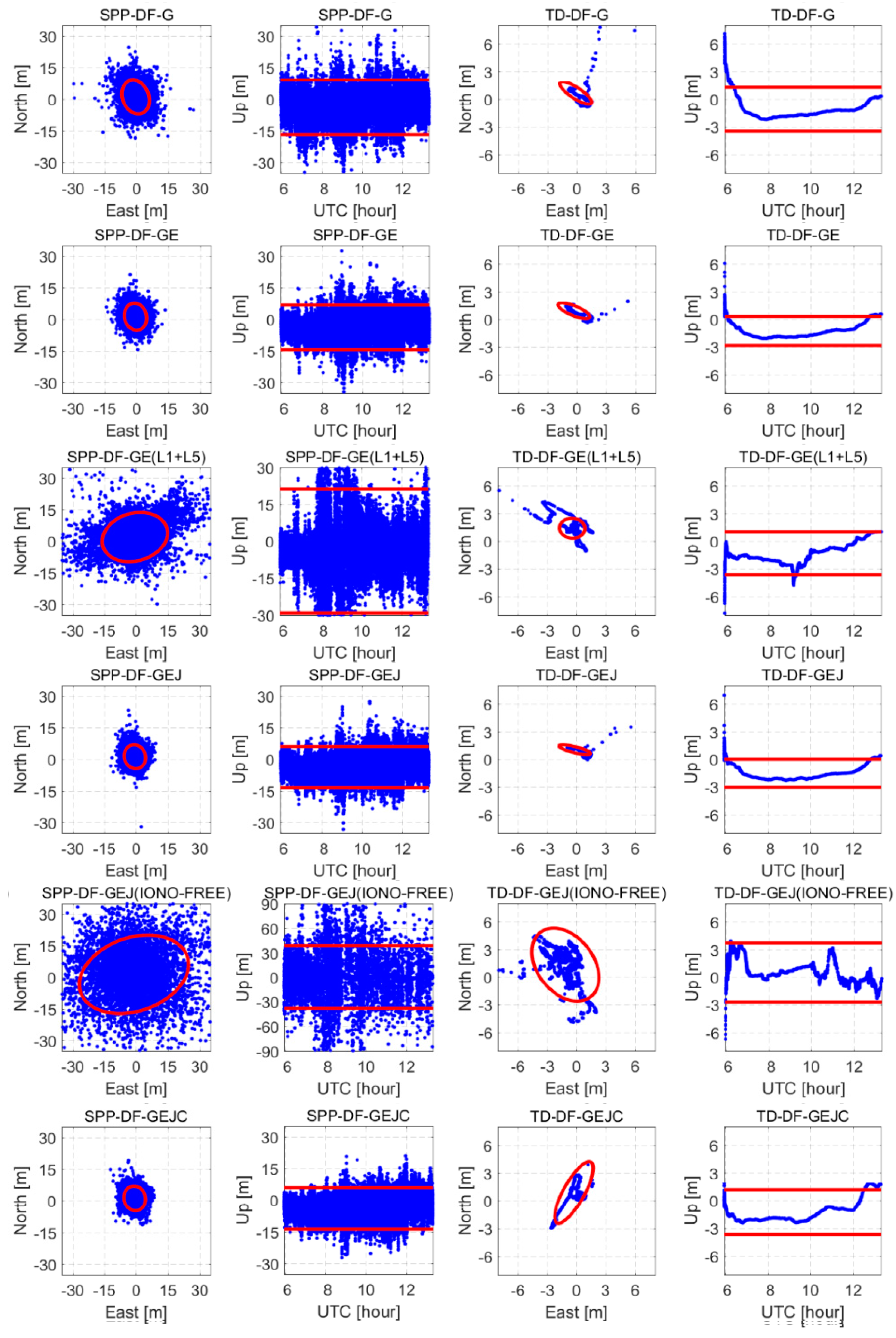
In order to analyze the achievable positioning performance by multi-system and dual-frequency observations, especially the newly added L5/E5 frequency in Xiaomi Mi 8, the GNSS observations were processed by SPP and the time differenced filter for the cases of GPS-only (G), GPS/Galileo (GE), GPS/Galileo/QZSS (GEJ), and GPS/Galileo/QZSS/BeiDou (GEJC) with single-frequency and dual-frequency observations. 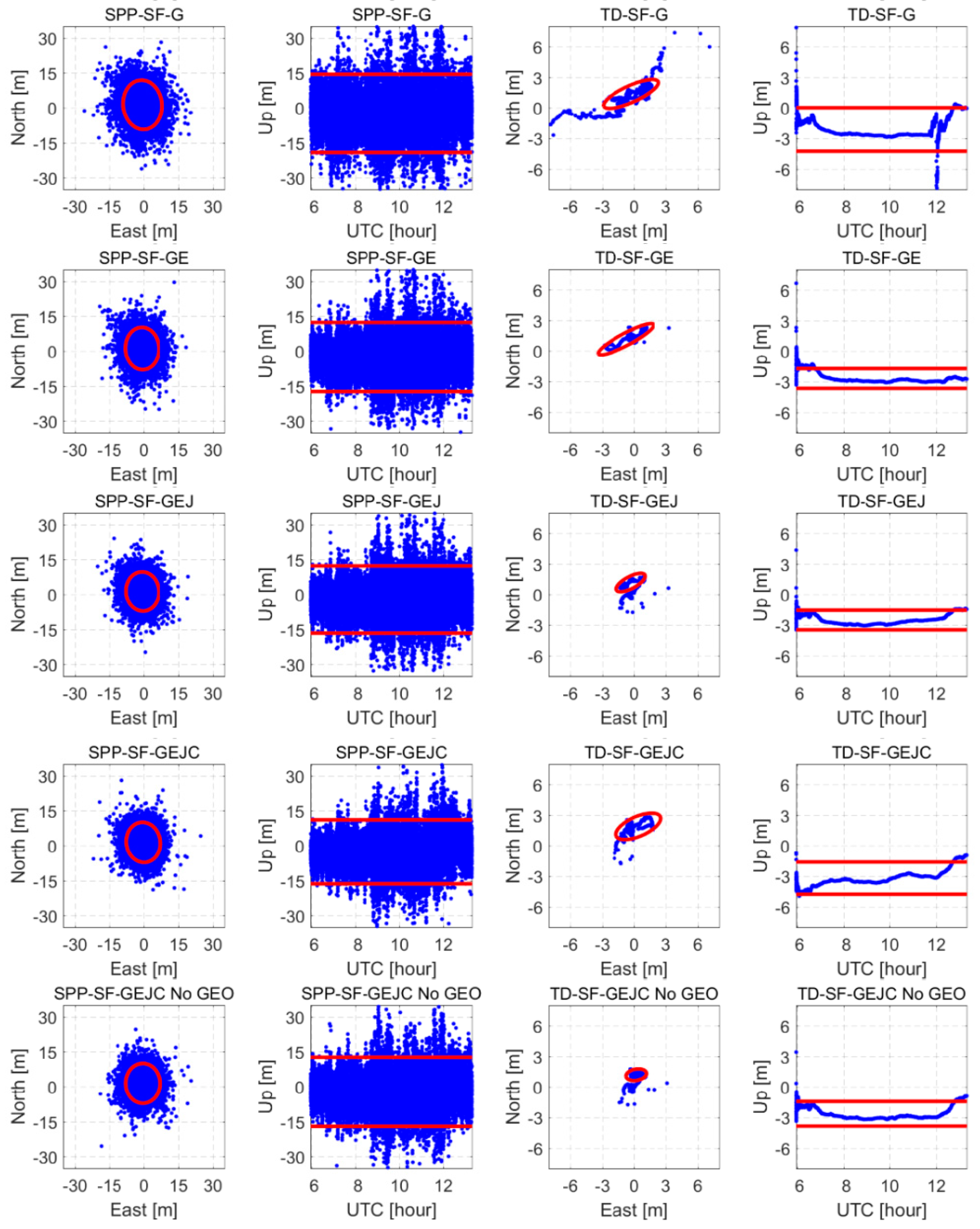The results are illustrated in Figure 14 and Figure 15. The horizontal position error scatters are shown in the odd columns while the vertical error scatters are shown in the even columns. The ellipses or straight lines inside each panel denote the 2σ domain of the scatters (95% confidence level). The smaller the ellipse is, the smaller the standard deviation, and the smoother the result. A comparison of the RMSs of the positioning errors is shown in

Table 4. RMS of TD filter and SPP solutions for Xiaomi Mi 8 in static test.

	TD Filter						SPP			SPP Availability (%)
	C/N0 Dependent			SISRE Based
	E (m)	N (m)	U (m)	E (m)	N (m)	U (m)	E (m)	N (m)	U (m)
SF 1-G	1.09	1.49	2.37				3.47	4.54	8.74	94.8
SF-GE	1.07	1.32	2.73	1.50	2.12	2.91	3.04	3.91	7.84	96.8
SF-GEJ	0.62	1.25	2.56	1.76	2.88	3.23	2.97	3.70	7.55	97.3
SF-GEJC 2	0.95	1.98	3.29	1.37	2.49	3.12	3.02	3.82	7.38	98.0
SF-GEJC without GEO	0.45	1.24	2.60	1.11	2.26	3.14	3.06	3.80	7.70	97.7
DF 3-G	0.67	0.92	1.64				2.62	3.46	7.37	97.9
DF-GE	0.67	0.87	1.48	0.77	1.76	1.87	2.18	2.95	6.53	99.3
DF-GE(L1+L5)	0.66	1.07	1.70	0.82	1.54	1.96	4.62	4.45	9.87	89.1
DF-GEJ	0.62	0.83	1.45	0.80	1.84	1.97	2.10	2.66	6.17	99.6
DF-GEJ(IONO-FREE)	1.71	2.04	1.63	1.69	2.85	2.04	5.17	5.32	8.67	63.5
DF-GEJC	0.84	1.62	1.46	0.85	1.94	1.84	2.15	2.68	6.18	99.7
DF-GEJC without GEO	0.61	0.92	1.40	0.73	1.84	1.84	2.19	2.68	6.21	99.7

¹ SF means only single frequency L1/E1 measurements are used for positioning; ² GEJC represent GPS/Galileo/QZSS/BeiDou, Separately; ³ DF means dual-frequency L1/E1 and L5/E5 measurements are used for positioning.

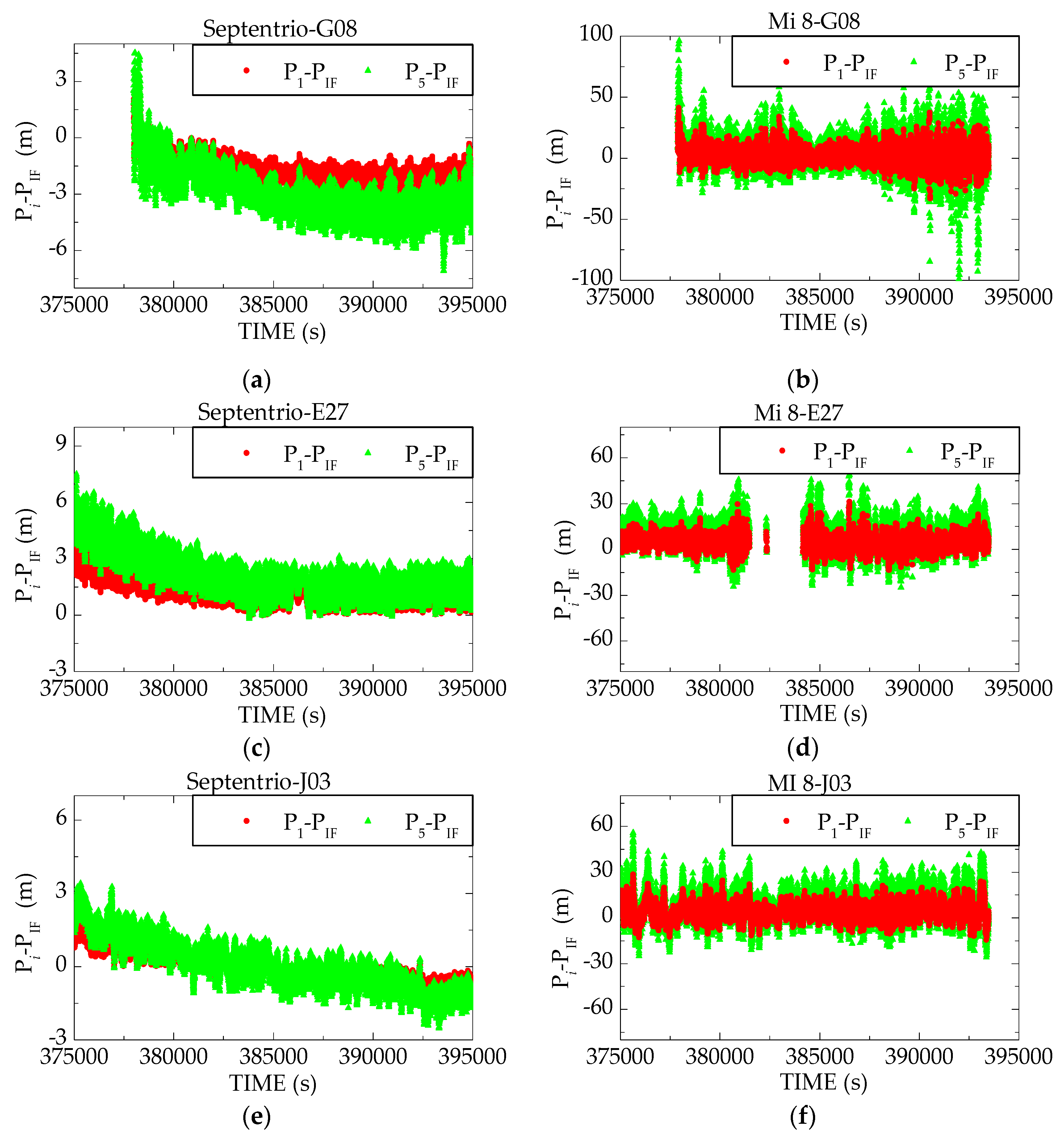
. We also calculated the solution availability, which is the percentage of solved positions that have a 3D error less than 20 m. Meanwhile, considering the advantage of the Galileo system and those GPS satellites with L5, we also conducted a positioning experiment using the Galileo and those GPS satellites with L5 measurements, labeled as ‘GE(L1+L5)’. Although, Figure 11 indicates that the ionosphere-free combination pseudorange may not be suitable for GNSS positioning with raw data from Xiaomi Mi 8 for its extreme large combined noise. Here we still conducted positing experiments with the dual-frequency ionosphere-free combined GPS, Galileo, and QZSS measurements to verify this, labeled as ‘GEJ(IONO-FREE)’.

It can be found that, for single-frequency SPP results, when the used navigation systems are increased, the RMS of the horizontal position errors decreases from 6 to 4 m, and 9 to 7 m for that of the vertical position errors. When using dual-frequency GNSS observations, the accuracy of SPP solutions improves slightly. The horizontal error RMS can be as good as 3.5 m, while the vertical error RMS is about 6.5 m. The increase in used navigation systems and inclusion of the second frequency have no obvious effect on the improvement of single-frequency SPP positioning accuracy, but the solution availability gets an effective boost. In the case of the single-frequency GEJC GNSS, the maximum solution availability can reach 98%. For dual-frequency GNSS cases, the positioning availability can be more than 99% when GPS and Galileo observations are used, and higher with the use of more systems. In short, the static data processing shows that, although the use of dual-frequency observations only has a slight improvement in the SPP accuracy, it strongly enhances the SPP solution availability.

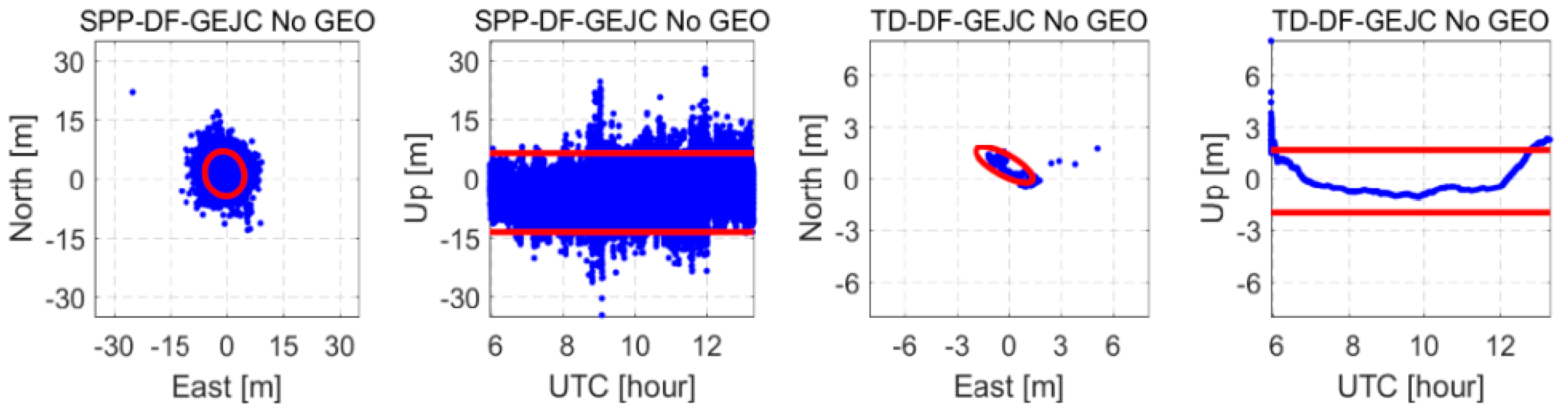
Looking into the results using the time differenced filter, we find that continuous and smooth positioning solutions are obtained for various observation combinations as shown in Figure 14 and Figure 15. When only L1/E1 observations are used, the horizontal error RMS is 1.5–2.0 m and the vertical error RMS is about 2.5 m. The use of dual-frequency GNSS observations reduces the horizontal error RMS to about 1.0 m, and the vertical error RMS to about 1.5 m. For the dual-frequency positioning results with Galileo and GPS measurements, it can be seen that when positioning with all Galileo and GPS satellites, the time differenced filter algorithm positioning error RMS in East (E), North (N) and Up (U) directions is 0.67 m, 0.87 m, and 1.48 m, respectively. The SPP positioning error RMS in E, N, and U is 2.18 m, 2.95 m, and 6.53 m, respectively. The SPP availability is 99.3%. However, when conducting with only the Galileo and those GPS satellites with L5 measurements, the time differenced filter algorithm positioning error is 0.66 m, 1.07 m, and 1.70 m in E, N, and U directions, respectively, which is slightly worse than the positioning results with all Galileo and GPS satellites. The SPP positioning error increased to 4.62 m, 4.45 m, and 9.87 m, and the SPP availability decreased to 89.1%. Clearly, as only a subset of GPS satellites transmits L5 signals, if use only Galileo satellites and those GPS satellites with L5, the number of usable satellites rapidly reduced and the navigation performance degraded. As to the dual-frequency positioning results with GPS, Galileo, and QZSS measurements, Figure 15 shows that the time differenced (TD) filter algorithm with a dual-frequency ionosphere-free combination positioning error RMS is 1.71 m, 2.04 m, and 1.63 m in E, N, and U directions, respectively; the SPP positioning error is 5.17 m, 5.32 m, and 8.67 m, respectively. These positioning errors are much larger than that of DF-GEJ results given by single-frequency positioning mode, as shown in Table 4. Clearly, the dual-frequency ionosphere-free combined measurements greatly amplified the pseudorange noise, and the positioning performance degraded. Thus, the ionosphere-free combination pseudorange is not suitable for GNSS positioning with raw data from Xiaomi Mi 8. When conducting single-frequency positioning with L1/E1 measurements or dual-frequency positioning with the uncombined L1/E1 and L5/E5 measurements, interestingly, whether using single-frequency or dual-frequency GNSS observations, the GEJ combination has the best positioning accuracy. When the BeiDou observations are included, the positioning accuracy decreases, and the horizontal error RMS is about 2 m. As the time differenced filter algorithm can smooth the noise of pseudorange observations, its positioning accuracy is mainly affected by the broadcast ephemeris error, satellite position dilution of precision (PDOP), and ionospheric delay error. According to the error analysis of the broadcast ephemeris of various navigation systems by Oliver Montenbruck et al. [37,38], the near-static observation geometry for BeiDou GEO satellites results in a degraded orbit determination accuracy in comparison with Inclined GeoSynchronous Orbit (IGSO) and Medium Earth Orbit (MEO) satellites. Its along-track component of GEO satellite orbits is the least well determined, with errors up to tens of meters, and typical signal-in-space range errors reaching 3 m. 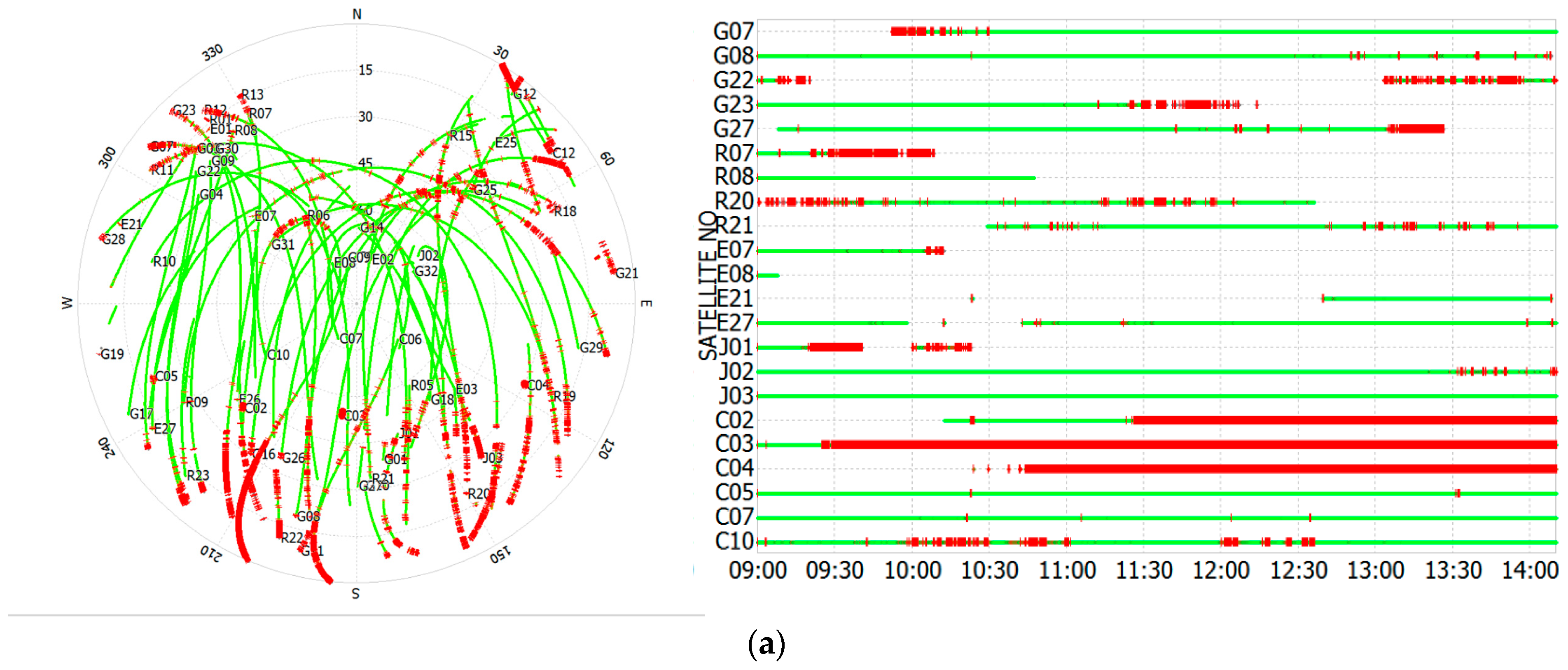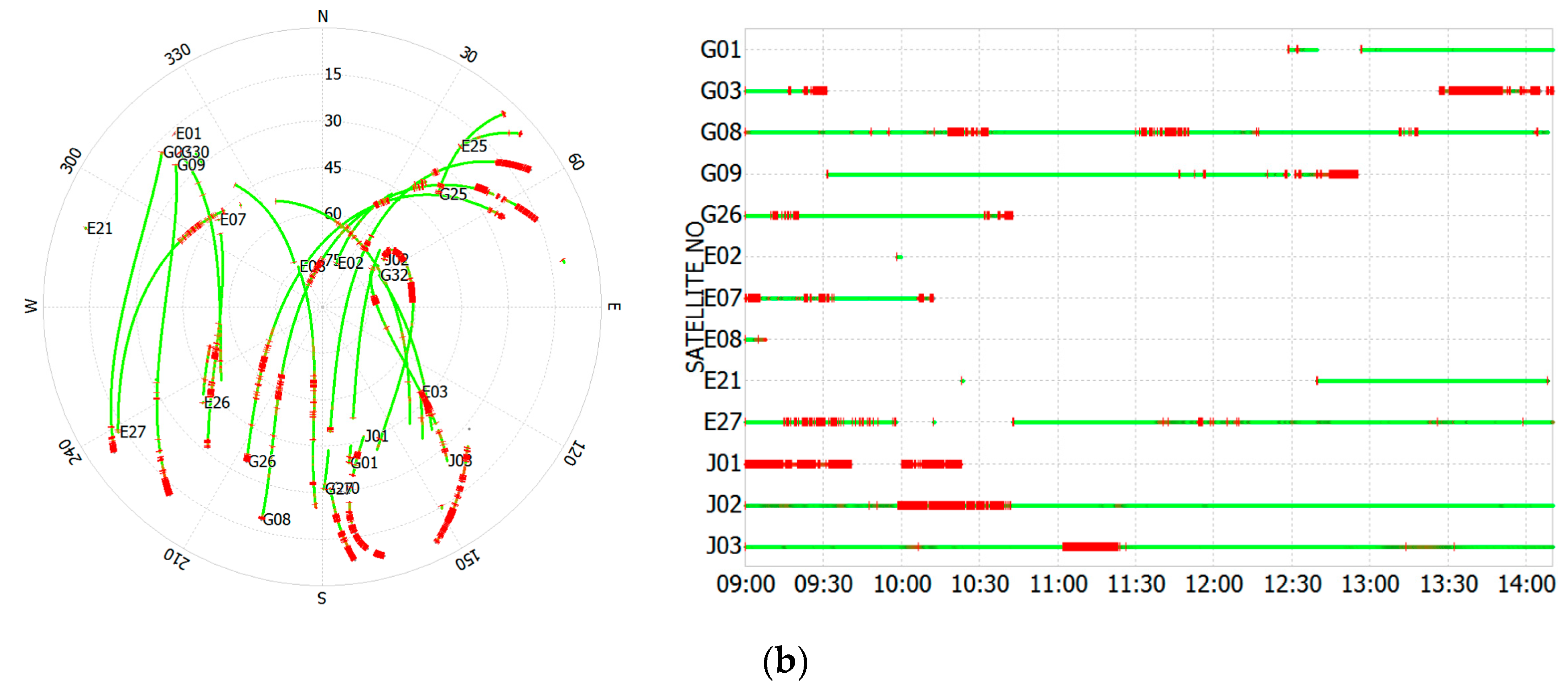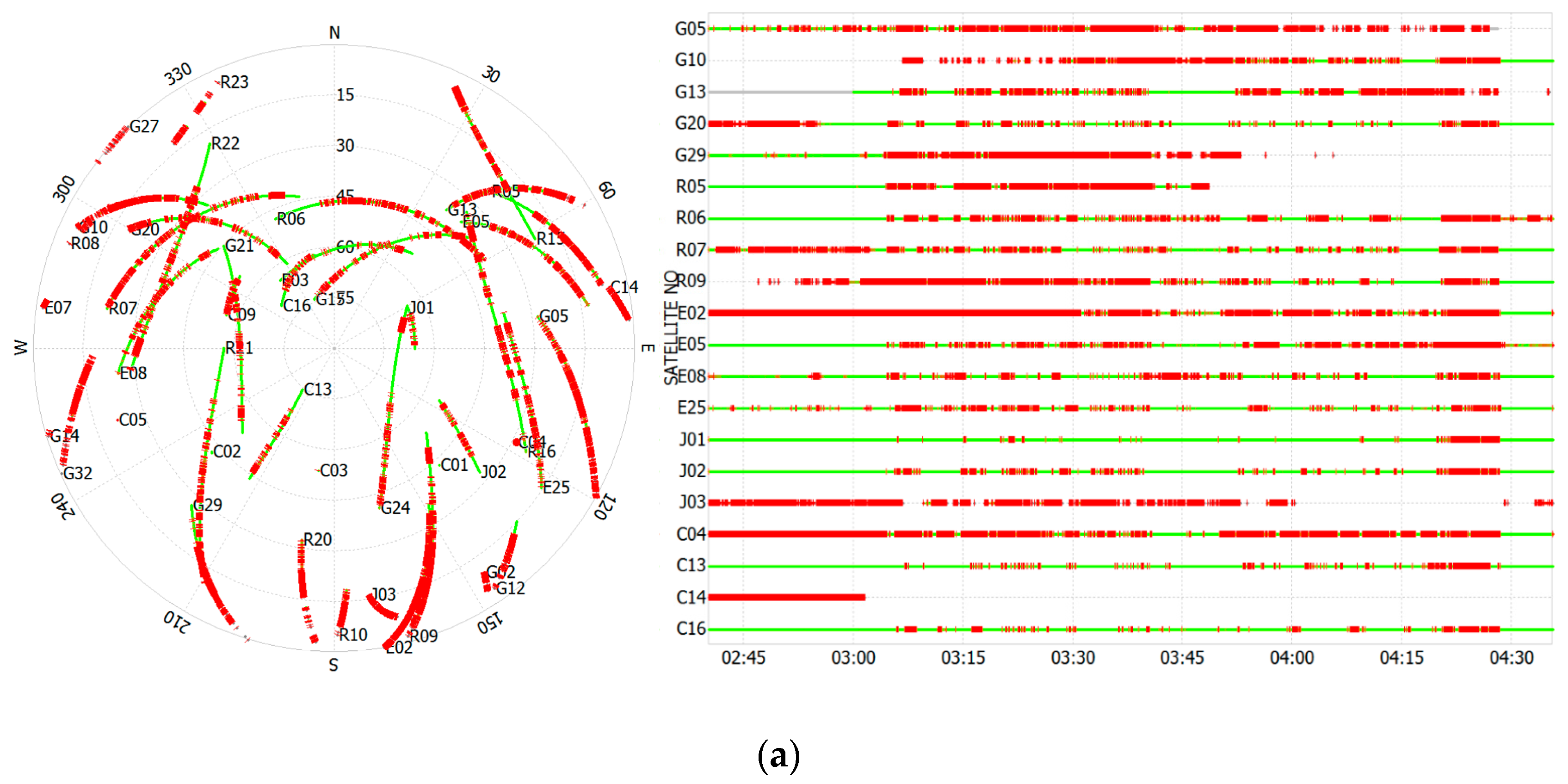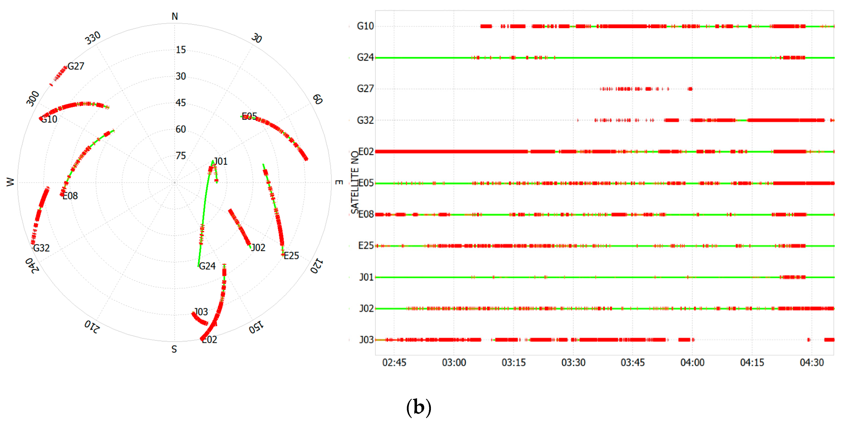In addition, Figure 2 shows that, under static conditions, four GEO satellites are observed. Therefore, it is reasonable to conclude that the positioning error increment is due to the inclusion of the BeiDou GEO data. To verify this point, we re-processed the same data but excluded BeiDou GEO satellites. The results are shown in the fifth row of Figure 14 and seventh row of Figure 15. It is clear that the horizontal error RMS decreases rapidly. In addition, as illustrated in Figure 2, the carrier phase observations of the BeiDou GEO satellites are interrupted much more often than those of other satellites. Therefore, when there are sufficient visible satellites, it is suggested that, for Xiaomi Mi 8, Beidou GEO satellites should not be used. 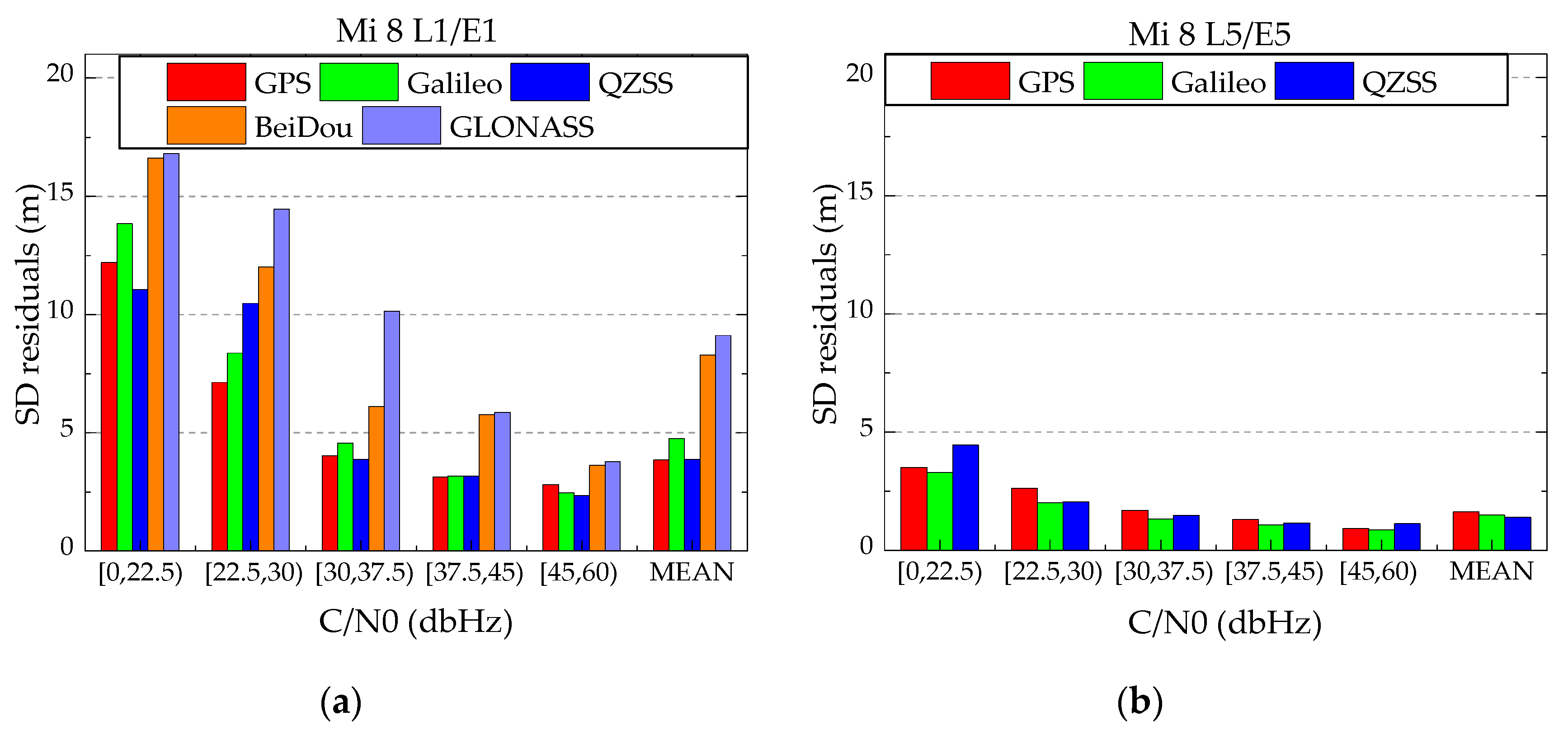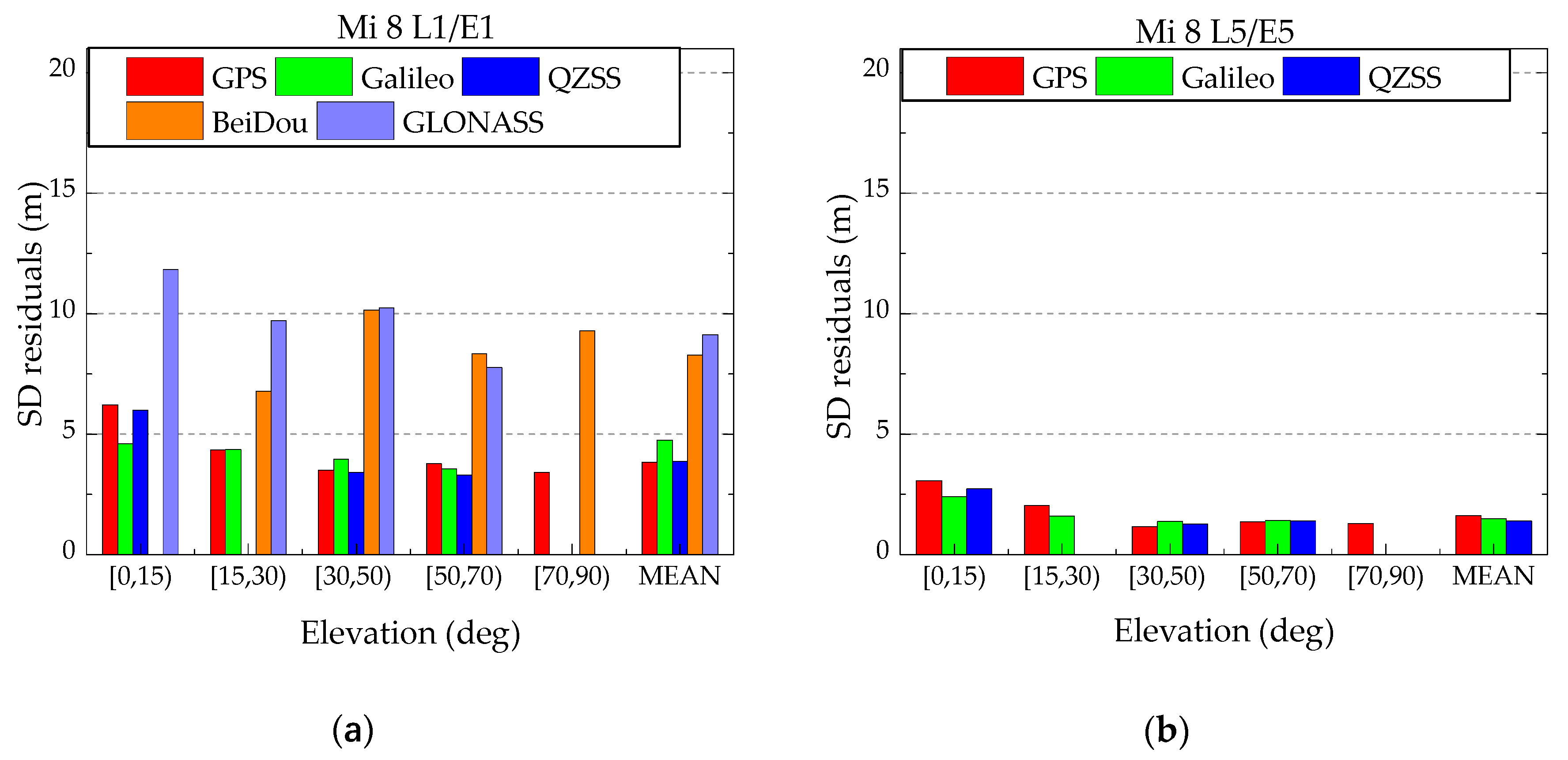Comparing the TD filter results of C/N0-dependent weighting with that of the SISRE value based weighting in Table 4, it can be seen that, the positioning accuracy of the SISRE value-based weighting is worse than that of the C/N0-dependent weighting model. The pseudorange noise is the major one in all error sources, and much larger than the errors of GNSS satellite orbits and clocks. 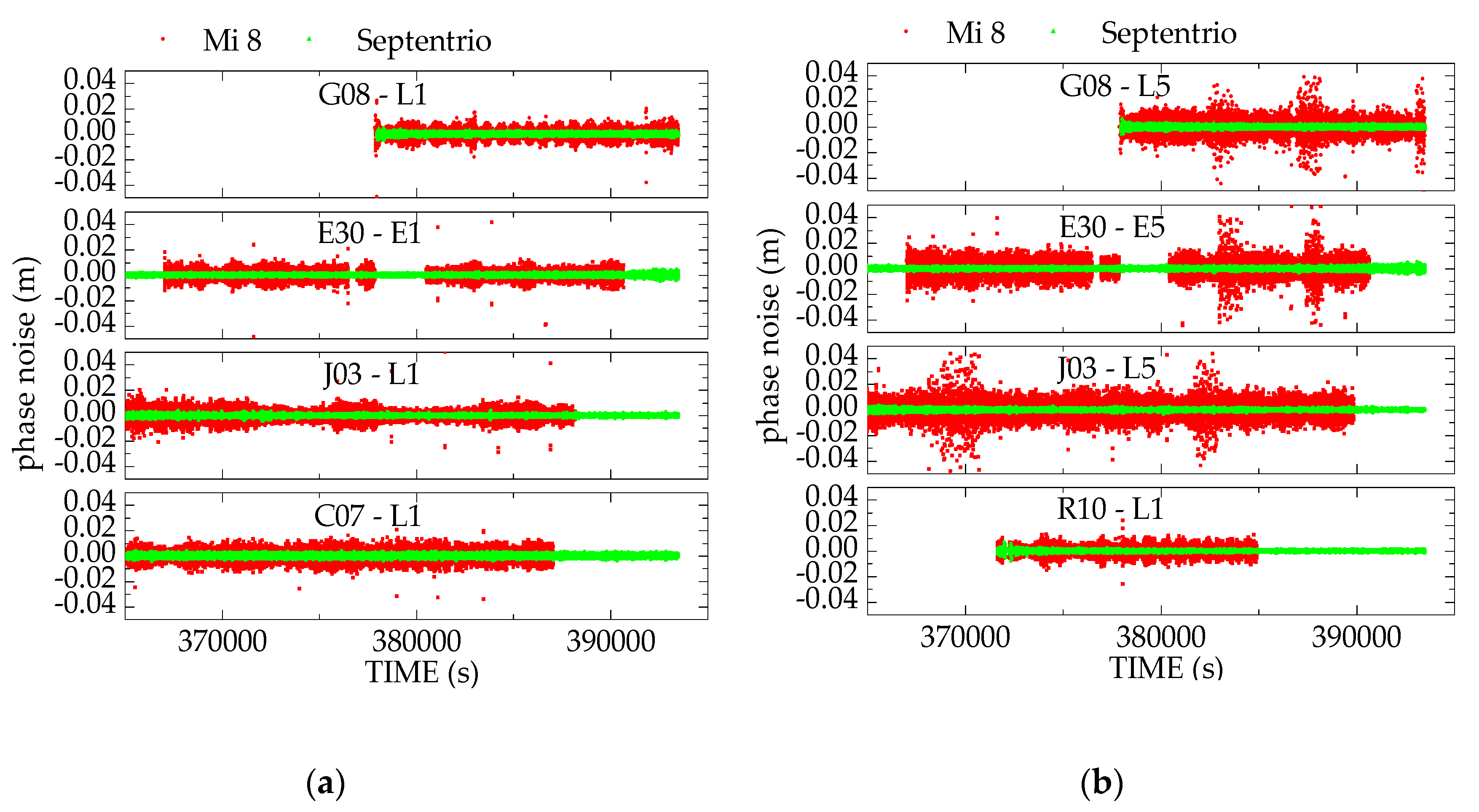A reasonable weighting model should be set based on the noise level of pseudorange observations, as the pseudorange noise is clearly related to the C/N0 as shown in Figure 9. Therefore, the C/N0-dependent weighting model is more suitable.

5.3. Dynamic Test Analysis

Figure 16 shows the trajectories of the time differenced filter kinematic solutions with respect to a combination of different systems and frequencies.

Table 5. RMS of time differenced filter solutions for Xiaomi Mi 8 in open environment (track 1).

Frequency-GNSS	E (m)	N (m)	U (m)	Availability (%)	Average Number of Observations
SF-G	2.391	3.268	5.698	62.1	5.9
SF-GE	0.508	1.601	2.835	85.8	9.4
SF-GEJ	0.482	1.379	1.810	88.3	11.5
SF-GEJC	0.489	1.392	1.831	92.9	14.2
DF-G	1.332	1.539	2.031	77.1	7.1
DF-GE	0.592	1.238	2.047	92.7	14.7
DF-GEJ	0.506	1.252	1.875	94.9	19.0
DF-GEJC	0.460	1.131	1.941	97.8	22.1

and

Table 6. RMS of TD filter solutions for Xiaomi Mi 8 in GNSS-degraded environment (track 2).

Frequency-GNSS	E (m)	N (m)	U (m)
SF-GEJC	0.830	1.973	4.115
DF-GEJC	0.713	1.442	2.156

give the statistical information of the navigation results under open-sky (track 1) and GNSS-degraded environments (track 2), respectively. For the mass-market navigation, the accuracy and availability of the navigation in the horizontal direction are usually more concerned. Here, the definition of the solution availability is made with a 5 m 2D accuracy criterion, instead of 20 m 3D accuracy in the static case. In addition, the average number of pseudorange observations in each solution is also given.

As illustrated in Figure 16 and Table 5 for track 1, with the increase of observations, the navigation performance of the time differenced filter is significantly improved, and the trajectories become very smooth. For the single-frequency case, continuous and smooth navigation results are obtained by only using GE satellites. Compared with the GPS-only solution, when using GEJC observations, the average number of used satellites increased to 14.2. The availability of navigation results increased from 62.1% to 92.9%, and the RMS of horizontal position errors decreased from 4.05 m to 1.48 m. When L5/E5 observations are available, the navigation performance is further improved, and the overall navigation trajectory is smoother than that of only using single-frequency observations. Here, even when only GE observations are used, the solution availability reaches 92.7%, which is nearly equivalent to that of single-frequency results with GEJC observations, and the RMS of horizontal position errors decreases to 1.68 m. In addition, when using dual-frequency GNSS observations of GREC satellites, the navigation availability is 97.8%. Correspondingly, the average number of used observations increases to 22.1, and RMS of the horizontal position errors is about 1.22 m.

The navigation results in the adverse GNSS environments of track 2 are given in Figure 16 and Table 6. Clearly, due to the unfavorable navigation environment, the navigation performance of Xiaomi Mi 8 rapidly deteriorates, and navigation trajectory jitters occur. For instance, even with the use of GEJC observations, the single-frequency navigation solutions still present obvious jitters, especially in areas with severe signal occlusion (between tall buildings and dense trees, the southern blue block in the Figure 16). The RMSs of position errors in the E, N, and U directions are 0.830 m, 1.973 m, and 4.115 m, respectively. The situation is obviously improved, when dual-frequency GNSS observations are used, as shown in the bottom four panels of Figure 16. It is seen that continuous and accurate navigation results are achieved even in the southern area where GNSS signals are severely degraded due to the tall buildings. The navigation accuracy is improved with the position RMSs in the E, N, and U directions reduced to 0.713 m, 1.442 m, and 2.156 m, respectively.

From the above analyses, it can be found that using multi-GNSS observations can effectively improve the accuracy and availability of mobile phone navigation. What is more important, the newly added second frequency L5/E5 observations, with their excellent observation accuracy, provide better location services in terms of navigation availability and positioning accuracy even in adverse GNSS environments.

Figure 17 shows the position dilution of precision (PDOP), the IEPV status, the number of observations collected, and the number of observations used in the two kinematic circuits with GEJC satellites and single-frequency and dual-frequency observations. Here, the IEPV status describes the way the IEPV, namely $\Delta {\mathrm{X}}_{t_{i-1},t_i}$ in Equation (7), is computed. If the IEPV status is 1, it indicates that the IEPV is calculated using the TDCP measurements, while 0 means there are not enough usable TDCP measurements to calculate the IEPV, and it is obtained by multiplying the Doppler-derived speed with $\Delta \mathrm{t}$. It can be seen in Figure 17 that, between three and six observations are eliminated during gross error detection. For single-frequency GNSS solutions, the mean value of PDOP in the open environment is about 2.45, and slightly increases to 2.62 in the GNSS-degraded environment; when using dual-frequency GNSS observations, the PDOP decreases further, reaching 1.89 in the open environment and 2.10 in the adverse GNSS environment. The four IEPV status sequences in Figure 17 illustrate that it remains 1 in the open environment, regardless of the use of single-frequency or dual-frequency GNSS observations. That is to say, in the open environments, the carrier phase observations are continuous and cycle slips are rare, and the IEPV is calculated successfully from phase differences between epochs. In track 2, however, if only single-frequency observations are used, many IEPV statuses are labeled 0, which means the IEPVs are calculated from the Doppler-derived velocity whose accuracy is usually lower than that calculated by time differenced carrier phases. For example, as shown in the upper red box in Figure 17, when Xiaomi Mi 8 is just between tall buildings and dense trees (same area in the red box in Figure 16), the IEPV status remains 0 for several consecutive epochs, meanwhile the number of used observations decreases and the PDOP value increases slightly. When the dual-frequency is available, only a few IEPV statuses are 0, and the PDOP over the navigation course is relatively stable. Clearly, the L5/E5 observations play an important role in improving the performance of mobile phone navigation in the complex environment.

6. Conclusions and Outlook

In this paper, we comprehensively analyzed the characteristics of raw GNSS observations from Xiaomi Mi 8, and conducted positioning experiments under open-static and dynamic GNSS-degraded environments. Firstly, we found that the C/N0 of the smart device is about 4 to 11 dBHz lower than those of geodetic receivers, and characterized by rapid variations. In addition, C/N0 are not significantly correlated to the satellite elevations. Secondly, we investigated the pseudorange and carrier phase observation error characteristics of Xiaomi Mi 8. The results show that the pseudorange noise of the L1/E1 observations is as high as 3~9 m in complex dynamic environments while that of L5/E5 observations is about 1.5 m. The correlation between the pseudorange noise and C/N0 is obvious, and a C/N0-dependent weight model is used for Xiaomi Mi 8 GNSS positioning. At the same time, we found that the pseudorange noise of Xiaomi Mi 8 is so large that the pseudorange ionosphere-free combination model is not suitable for Xiaomi Mi 8 GNSS positioning. As to the carrier phase observations, the observation noise is about 2 cm, but the cycle slip percentages of carrier phase observations are quite high in dynamic tests, rising to 62.25% in GNSS-degraded environments. Therefore, in order to effectively utilize the high precision carrier phase observations, a time differenced positioning filter is proposed to deliver continuous and smooth navigation results in urban GNSS-degraded environments.

Finally, the single-device positioning performance of Xiaomi Mi 8 using a time differenced filter was investigated, especially the positioning performance improvement with the inclusion of L5/E5 observations in GNSS-degraded environments. The RMSs of the horizontal and vertical position errors can be as small as 1.0 m and 1.5 m, respectively, using multi-system dual-frequency GNSS observations under static conditions. In the dynamic open environment, the average number of used observations was about 22.1, the RMS of horizontal errors was about 1.22 m, and the navigation availability reached 97.8%. Correspondingly, under the adverse GNSS environments, the horizontal navigation accuracy was about 1.61 m when L5/E5 observations were available. Clearly, this TD filter algorithm can deliver satisfied positioning results for various LBSs. It can also be expanded to newly emerged applications, like augmented reality, seamless image-based navigation, and photogrammetric data collection applications in complex environments.

The L5/E5 signal from Xiaomi Mi 8 has outstanding characteristics, and provides better location services in terms of positioning availability and accuracy even in GNSS-degraded environments. Nevertheless, due to the vulnerability of the GNSS signal, work on multi-sensor fusion (such as GNSS/MEMS fusion) for the pedestrian navigation is underway to ensure continuous navigation in a GNSS signal denied environment.

References

1. The European GNSS Agency. GNSS Market Report 2017; The European GNSS Agency: Prague, Czech Republic, May 2017.
2. Zhang, X.; Tao, X.; Feng, Z.; Xiang, S.; Wang, F. Quality assessment of GNSS observations from an Android N smartphone and positioning performance analysis using time-differenced filtering approach. GPS SOLUT 2018, 22, 70. [Google Scholar] [CrossRef]
3. Küpper, A. Location-Based Services: Fundamentals and Operation; John Wiley & Sons: Hoboken, NJ, USA, 2005. [Google Scholar]
4. Li, P.; Qin, T.; Hu, B.; Zhu, F.; Shen, S. Monocular Visual-Inertial State Estimation for Mobile Augmented Reality. In Proceedings of the 2017 IEEE International Symposium on Mixed and Augmented Reality (ISMAR), Nantes, France, 9–13 October 2017. [Google Scholar]
5. Piras, M.; Lingua, A.; Dabove, P.; Aicardi, I. Indoor navigation using Smartphone technology: A future challenge or an actual possibility? In Proceedings of the 2014 IEEE/ION Position, Location and Navigation Symposium—PLANS 2014, Monterey, CA, USA, 5–8 May 2014. [Google Scholar]
6. Kim, J.; Lee, S.; Ahn, H.; Seo, D.; Park, S.; Choi, C. Feasibility of employing a smartphone as the payload in a photogrammetric UAV system. ISPRS J. Photogramm. Remote Sens. 2013, 79, 1–18. [Google Scholar] [CrossRef]
7. Liu, W.; Shi, X.; Zhu, F.; Tao, X.; Wang, F. Quality analysis of multi-GNSS raw observations and a velocity-aided positioning approach based on smartphones. Adv. Space Res. 2019, 63, 2358–2377. [Google Scholar] [CrossRef]
8. Pesyna, K.M.; Humphreys, T.E.; Heath, R.W.; Novlan, T.D.; Zhang, J.C. Exploiting antenna motion for faster initialization of centimeter accurate GNSS positioning with low-cost antennas. IEEE Trans. Aerosp. Electron. Syst. 2017, 53, 1597–1613. [Google Scholar] [CrossRef]
9. Li, G.; Geng, J. Characteristics of raw multi-GNSS measurement error from Google Android smart devices. GPS Solut. 2019, 23, 90. [Google Scholar] [CrossRef]
10. Banville, S.; Diggelen, F. Precise GNSS for Everyone: Precise Positioning Using Raw GPS Measurements from Android Smartphones. GPS World 2016, 27, 43–48. [Google Scholar]
11. Realini, E.; Caldera, S.; Pertusini, L.; Sampietro, D. Precise GNSS Positioning Using Smart Devices. Sensors 2017, 17, 2434. [Google Scholar] [CrossRef] [PubMed] [Green Version]
12. Dabove, P.; Di Pietra, V. Towards high accuracy GNSS real-time positioning with smartphones. Adv. Space Res. 2019, 63, 94–102. [Google Scholar] [CrossRef]
13. Gogoi, N.; Minetto, A.; Linty, N.; Dovis, F. A Controlled-Environment Quality Assessment of Android GNSS Raw Measurements. Electronics 2019, 8, 5. [Google Scholar] [CrossRef] [Green Version]
14. Riley, S.; Lentz, W.; Clare, A. On the Path to Precision - Observations with Android GNSS Observables. In Proceedings of the 30th International Technical Meeting of the Satellite Division of the Institute of Navigation, Portland, OR, USA, 25–29 September 2017. [Google Scholar]
15. Staff, G.W. World’s First Dual-Frequency GNSS Smartphone Hits the Market. Available online: https://www.gpsworld.com/dual-frequency-gnss-smartphone-hits-the-market/ (accessed on 10 September 2019).
16. Marco, F.; Joshua, C.; Malgorzata, S.; Maria, L.; Elisa, B.; William, R. Enabling High Accuracy Dynamic Applications in Urban Environments Using PPP and RTK on Android Multi-Frequency and Multi-GNSS Smartphones. In Proceedings of the 2019 European Navigation Conference (ENC), Warsaw, Poland, 9–12 April 2019. [Google Scholar]
17. Crosta, P.; Zoccarato, P.; Lucas, R.; Pasquale, G. Dual Frequency Mass-market Chips: Test Results and Ways to Optimize PVT Performance. In Proceedings of the 31st International Technical Meeting of The Satellite Division of the Institute of Navigation (ION GNSS+ 2018), Miami, FL, USA, 24–28 September 2018. [Google Scholar]
18. Moore, S.K. Super-accurate GPS coming to smartphones in 2018. IEEE Spectr. 2017, 54, 10–11. [Google Scholar] [CrossRef]
19. Shade, S.; Madhani, P. Android GNSS Measurements - Inside the BCM47755. In Proceedings of the 31st International Technical Meeting of the Satellite Division of the Institute of Navigation (ION GNSS+ 2018), Miami, FL, USA, 24–28 September 2018. [Google Scholar]
20. Robustelli, U.; Baiocchi, V.; Pugliano, G. Assessment of Dual Frequency GNSS Observations from a Xiaomi Mi 8 Android Smartphone and Positioning Performance Analysis. Electronics 2019, 8, 91. [Google Scholar] [CrossRef] [Green Version]
21. Wu, Q.; Sun, M.; Zhou, C.; Zhang, P. Precise Point Positioning Using Dual-Frequency GNSS Observations on Smartphone. Sensors 2019, 19, 2189. [Google Scholar] [CrossRef] [PubMed] [Green Version]
22. Elmezayen, A.; El-Rabbany, A. Precise Point Positioning Using World’s First Dual-Frequency GPS/GALILEO Smartphone. Sensors 2019, 19, 2593. [Google Scholar] [CrossRef] [PubMed] [Green Version]
23. Chen, B.; Gao, C.; Liu, Y.; Sun, P. Real-time Precise Point Positioning with a Xiaomi MI 8 Android Smartphone. Sensors 2019, 19, 2835. [Google Scholar] [CrossRef] [Green Version]
24. Takasu, T. RTKLIB Ver. 2.4. 2. Available online: https://github.com/tomojitakasu/RTKLIB_bin/tree/rtklib_2.4.3 (accessed on 15 November 2019).
25. White Paper on Using GNSS Raw Measurements on Android Devices; European GNSS Agency: Prague, Czech Republic, 2017.
26. Joseph, A. What is the difference between SNR and C/N0? InsideGNSS 2010, 5, 20–25. [Google Scholar]
27. Hauschild, A.; Montenbruck, O.; Sleewaegen, J.M.; Huisman, L.; Teunissen, P.J.G. Characterization of Compass M-1 signals. GPS Solut. 2012, 16, 117–126. [Google Scholar] [CrossRef]
28. Amiri-Simkooei, A.R.; Tiberius, C.C.J.M. Assessing receiver noise using GPS short baseline time series. GPS Solut. 2007, 11, 21–35. [Google Scholar] [CrossRef] [Green Version]
29. Teunissen, P.J.G.; Montenbruck, O. Springer Handbook of Global Navigation Satellite Systems; Springer International Publishing: Cham, Switzerland, 2017. [Google Scholar]
30. Pirazzi, G.; Mazzoni, A.; Biagi, L.; Crespi, M. Preliminary performance analysis with a GPS+Galileo enabled chipset embedded in a smartphone. In Proceedings of the 30th International Technical Meeting of the Satellite Division of the Institute of Navigation (ION GNSS+ 2017), Portland, OR, USA, 25–29 September 2017. [Google Scholar]
31. Traugott, J. Precise Flight Trajectory Reconstruction Based on Time-Differential GNSS Carrier Phase Processing. Bachelor’s Thesis, Technical University of Munich, Munich, Germany, 28 October 2010. [Google Scholar]
32. Wang, F.; Gong, X.; Sang, J.; Zhang, X. A Novel Method for Precise Onboard Real-Time Orbit Determination with a Standalone GPS Receiver. Sensors 2015, 15, 30403–30418. [Google Scholar] [CrossRef] [Green Version]
33. Carcanague, S. Low-Cost GPS/GLONASS Precise Positioning Algorithm in Constrained Environment. Ph.D. Thesis, Institut National Polytechnique de Toulouse—INPT, Toulouse, France, 25 February 2014. [Google Scholar]
34. Cabinet Office; Quasi-Zenith Satellite System Services Inc. Quasi-Zenith Satellite System Interface Specification Satellite Positioning, Navigation and Timing Service (IS-QZSS-PNT-003). 2018. Available online: https://qzss.go.jp/en/technical/ps-is-qzss/ps-is-qzss.html (accessed on 24 February 2020).
35. Saastamoinen, J. Contributions to the theory of atmospheric refraction. Bull. Géodésique 1973, 107, 13–34. [Google Scholar] [CrossRef]
36. Kazmierski, K.; Hadas, T.; Sośnica, K. Weighting of Multi-GNSS Observations in Real-Time Precise Point Positioning. Remote Sens. 2018, 10, 84. [Google Scholar] [CrossRef] [Green Version]
37. Montenbruck, O.; Steigenberger, P.; Hauschild, A. Broadcast versus precise ephemerides: A multi-GNSS perspective. GPS Solut. 2015, 19, 321–333. [Google Scholar] [CrossRef]
38. Montenbruck, O.; Steigenberger, P.; Hauschild, A. Multi-GNSS signal-in-space range error assessment—Methodology and results. Adv. Space Res. 2018, 61, 3020–3038. [Google Scholar] [CrossRef]
Figure 1. Static data collecting environments on the roof of Wuhan University School of Geodesy and Geomatics building.
Remotesensing 12 00744 g001
Figure 2. Sky plots and ADRS of observed Global Navigation Satellite System (GNSS) satellites by Xiaomi Mi 8 in static test. (a) is for L1/E1 measurements. (b) is for L5/E5 measurements. The short red line is the ADRS field provided by an Android smartphone.
Remotesensing 12 00744 g002aRemotesensing 12 00744 g002b
Figure 3. Trajectory of the utility cart obtained by NovAtel’s SPAN GNSS Inertial Navigation System. In track 2, due to the severe GNSS signal occlusion by dense trees and high buildings, fewer GPS + GLONASS) measurements are available. The NovAtel’s SPAN GNSS Inertial Navigation System derived trajectory has an obvious deviation to the reference points.
Remotesensing 12 00744 g003
Figure 4. Utility cart with NovAtel’s SPAN GNSS Inertial Navigation System and Xiaomi Mi 8.
Remotesensing 12 00744 g004
Figure 5. Sky plots and ADRS of observed GNSS satellites by Xiaomi Mi 8 in dynamitic test. (a) is for L1/E1 measurements. (b) is for L5/E5 measurements. The short red line is the ADRS field provided by an Android smartphone.
Remotesensing 12 00744 g005aRemotesensing 12 00744 g005b
Figure 6. Normalized histograms displaying the drop in C/N0 between a survey-grade antenna and Xiaomi Mi 8 antenna of L1/E1. The red histograms are the C/N0 drop between the two Septentrio receivers. The green histograms are the C/N0 drop between the Xiaomi Mi 8 and a Septentrio receiver. (a) is about GPS L1 measurements. (b) is about GLONASS L1 measurements. (c) is about Galileo E1 measurements. (d) is about BeiDou L1 measurements. (e) is about QZSS L1 measurements.
Remotesensing 12 00744 g006
Figure 7. Normalized histograms displaying the drop in carrier-to-noise ratio between a survey-grade antenna and Xiaomi Mi 8 antenna of L5/E5. (a) is about GPS L5 measurements. (b) is about Galileo E5 measurements. (c) is about QZSS L5 measurements.
Remotesensing 12 00744 g007
Figure 8. Average C/N0 values against the satellite elevations for Septentrio and Xiaomi Mi 8 on L1/E1 and L5/E5. The C/N0 values within an elevation range of 1° are averaged.
Remotesensing 12 00744 g008
Figure 9. Root mean square (RMS) statistics of the GPS/Galileo/QZSS/BeiDou/GLONASS L1/E1 (a) and L5/E5 (b) SD pseudorange residuals against the C/N0 for dynamic data (track 1).
Remotesensing 12 00744 g009
Figure 10. RMS statistics of the GPS/Galileo/QZSS/BeiDou/GLONASS L1/E1 (a) and L5/E5 (b) SD pseudorange residuals against the elevation for dynamic data (track 1).
Remotesensing 12 00744 g010
Figure 11. Differences of raw pseudorange measurements and the ionosphere-free combination pseudorange measurements for Septentrio receivers about satellites (a) G08, (c) E27, (e) J03 and Xiaomi Mi 8 about satellite (b) G08, (d) E27, (f) J03, respectively. Pi (i = 1, 5) are L1/E1 and L5/E5 pseudorange measurements, respectively. PIF means ionosphere-free combination pseudorange measurements.
Remotesensing 12 00744 g011
Figure 12. The carrier phase noise comparison of Xiaomi Mi 8 and Septentrio receiver for satellites G08/E30/J03/C07/R10 about (a) L1/E1 and (b) L5/E5 measurements. The carrier phase noises of Xiaomi Mi 8 are shown by red dots, and the carrier phase noises of the Septentrio receiver are shown by green dots.
Remotesensing 12 00744 g012
Figure 13. Flow chart of the time differenced filter algorithm.
Remotesensing 12 00744 g013
Figure 14. Positioning errors of single frequency time differenced (TD) filter and SPP solutions for Xiaomi Mi 8 with L1/E1 measurements in open-sky rooftop situations. The horizontal position scatters are shown in the odd columns, while the vertical scatters are shown in the even columns. The concentric ellipses or straight lines inside each panel denote the 2σ domain of the scatters.
Remotesensing 12 00744 g014
Figure 15. Positioning errors of double frequency TD filter and SPP solutions for Xiaomi Mi 8 in open-sky rooftop situations. The horizontal position scatters are shown in the odd columns, while the vertical scatters are shown in the even columns. The concentric ellipses or straight lines inside each panel denote the 2σ domain of the scatters. ‘GE(L1+L5)’ indicates the positioning results using Galileo and those GPS satellites with L5 measurements. ’GEJ(IONO-FREE)’ is the positioning results with the dual-frequency ionosphere-free combined GPS, Galileo, and QZSS measurements. ‘No GEO’ means the positioning results are generated by excluding Beidou GEO satellites.
Remotesensing 12 00744 g015aRemotesensing 12 00744 g015b
Figure 16. Trajectory of the kinematic solutions of different systems and frequencies. The blue rectangles indicate the area where the GNSS signals are severely degraded due to the tall buildings.
Remotesensing 12 00744 g016
Figure 17. PDOP, the IEPV status, the number of observations collected, and the number of observations used in the positioning solution. (a,b) represent the status of kinematic solutions with GEJC systems and single frequency observations in the open and GNSS-degraded environments, respectively. Correspondingly, (c,d) give the status with GEJC systems and dual-frequency observations in track 1 and track 2. The red line is the number of the used observations. The blue line is the number of the viewed observations. The green line is the PDOP. The black line is the IEPV status.
Remotesensing 12 00744 g017