Drone-borne Differential SAR Interferometry

Abstract

Differential synthetic aperture radar interferometry (DInSAR) has been widely applied since the pioneering space-borne experiment in 1989, and subsequently with the launch of the ERS-1 program in 1992. The DInSAR technique is well assessed in the case of space-borne SAR data, whereas in the case of data acquired from aerial platforms, such as airplanes, helicopters, and drones, the effective application of this technique is still a challenging task, mainly due to the limited accuracy of the information provided by the navigation systems mounted onboard the platforms. The first airborne DInSAR results for measuring ground displacement appeared in 2003 using L- and X-bands. DInSAR displacement results with long correlation time in P-band were published in 2011. This letter presents a SAR system and, to the best of our knowledge, the first accuracy assessment of the DInSAR technique using a drone-borne SAR in L-band. A deformation map is shown, and the accuracy and resolution of the methodology are presented and discussed. In particular, we have obtained an accuracy better than 1 cm for the measurement of the observed ground displacement. It is in the same order as that achieved with space-borne systems in C- and X-bands and the airborne systems in X-band. However, compared to these systems, we use here a much longer wavelength. Moreover, compared to the satellite experiments available in the literature and aimed at assessing the accuracy of the DInSAR technique, we use only two flight tracks with low time decorrelation effects and not a big data stack, which helps in reducing the atmospheric effects.

1. Introduction

Differential synthetic aperture radar interferometry (DInSAR) became popular after the launch of the ERS-1 satellite in 1991. Relevant satellite-borne DInSAR results already appeared in 1989 when Gabriel et al. [1] made two interferograms from three SAR images, taken from the same area at different times. They produced a double-difference interferogram to remove phase shifts caused by topography and to retain phase changes due to surface motion; they were able to measure surface motions of up to 1 cm with a 10-m resolution over 50 km swaths. Since then, a large number of deformation maps, generated from satellite-borne DInSAR data, have been supporting many geological and engineering monitoring tasks and studies. Nonetheless, satellite-borne DInSAR systems present an operational limitation due to the fixed orbits of the satellites, as DInSAR only measures displacement in the line-of-sight direction, and to retrieve a 3-D deformation map, information from at least three viewing angles is required. Some methods accomplish this by acquiring quasi-simultaneous SAR images with different squint angles [2,3]. Other methods use multi-interferograms from more than three directions [4] or the multiple aperture interferometry technique [5,6], which measures displacement in the along-track direction.

Airborne DInSAR for displacement measurements was first presented in 2003 using L-band [7], in 2004 using X-band [8], and in 2011 using P-band [9]. The first report of a controlled accuracy measurement using corner reflectors and distributed targets on the ground was published in 2008 [10]. Since aircraft have flexible flight patterns, surveying the area in three different directions is not a complicated task; therefore, generating 3-D deformation maps with airborne DInSAR is more straightforward than with satellite-borne systems. Moreover, brief revisit periods with high spatial resolution can be achieved. The airborne DInSAR solution has been implemented with limitation due to the high survey costs and the smaller illumination swath width, compared with satellite-borne systems. Additionally, aircraft movement caused by air turbulence is a hindrance to accurately executing airborne DInSAR, and hence many motion compensation techniques have been applied. Instead, Cao et al. [11] used the time-domain back-projection algorithm for SAR processing, which is intrinsically able to balance out platform motion. They demonstrated that it is possible to measure deformation with centimeter accuracy.

A novel drone-borne SAR system operating in the P-, L-, and C-bands and optimized for the DInSAR operation was presented in 2019 [12]. This new SAR system has a much smaller swath width when compared with airborne DInSAR systems and can cover areas of about tens of square kilometers. Thus, small-size drone-borne DInSAR systems are suitable for applications never attended by satellite and airborne DInSAR. A first DInSAR demonstration is introduced in [12], which had an RMS displacement measurement error of 0.045 m in L-band.

Deformation maps accurate to the order of a few millimeters are very useful as input to early warning systems for landslide and dam failure processes, or emergency management systems after earthquakes. The five most important features for having good differential interferometry results are high signal-to-noise ratio, low time decorrelation between the revisits, high radar and processing phase stability, interference-free antennae environment, and precise motion data. Each of these points will be quantitatively addressed.

This letter reports the first results of the drone-borne DInSAR obtained from a controlled experiment with a set of corner reflectors. During each of three subsequent flights, one of the corner reflectors was displaced, while the others remained fixed. The displacement measurement was six times more accurate than that presented in [12].

2. Materials and Methods

The radar prototype described in [12] operates in three bands: P, L, and C. Also, five channels are available: two C-band antennae for cross-track interferometry, two L-band antennae for polarimetry, and one P-band antenna. The results presented in this letter focus on the L-band HH-polarization for the DInSAR, in which the radar transmits and receives horizontally polarized waves.

Table 1. Main radar acquisition parameters.

Radar Parameters	Value
Carrier Wavelength	22.84 cm
Bandwidth	150 MHz
Polarization	HH
Peak Power	100 mW
Mean Power	1 mW
PRF	10 kHz
Incidence Angle	45 deg.
Mean Drone Height	120 m
Mean Drone Velocity	2 m/s
Motion Sensing System (MSS)	D-GNSS+IMU
Range Resolution	1 m
Azimuth Resolution	0.1 m
Processed Azimuth Bandwidth	20 Hz
Processed Aperture at 45 deg. Incidence Angle	196 m
SLC Range Sampling	0.61 m
SLC Azimuth Sampling	0.05 m

shows the main radar acquisition parameters.

The digital surface model (DSM) is determined by using the cross-track interferometry information provided by the two C-band antennae. Then, the DSM is applied in the DInSAR calculation. The nominal height accuracy is better than 1 m RMS with a spatial resolution of 2 m.

The motion sensing system (MSS) is integrated into the radar, as shown in [12], and it consists of a single channel GNSS receiver and an inertial measurement unit (IMU). One ground station with a single channel GNSS receiver is also utilized to allow differential GNSS processing.

Table 2. Accuracy specifications of the adopted motion sensing system (MSS) [12].

MSS Accuracy Specifications	Value
Position, Absolute	0.015 m
Position, Relative	<0.01 m
Roll and Pitch	0.1 deg.
True Heading	2 deg.
IMU Run Bias Stability	2 deg./h
IMU Angular Random Walk	0.1 deg./square root hour

shows the MSS requirements [12].

This letter shows the tests and the results of an L-band drone-borne DInSAR survey carried out at the University of Campinas, UNICAMP, Campinas, Brazil. Three trihedral corner reflectors with square sides and an edge length of 0.6 m were used as a ground reference. The resulting radar cross-section is 20 dB. Considering a 1-square-meter resolution cell, the respective sigma zero is 20 dB as the ground reflectivity has a sigma zero of about −5 dB.

The experiment with the drone-borne system, shown in Figure 1a, took place on 19 December 2018 at the UNICAMP test site, as follows.

• The GNSS ground station was placed close to the starting position of the drone, and the GNSS recording was initiated.
• Three flights were carried out, each consisting of the following successive steps: turning on the drone and the radar; waiting 15 min for simultaneous and stationary recording of ground station and radar GNSS data; take-off; executing the same west-east flight track; landing; waiting 15 min for simultaneous and stationary recording of ground station and radar GNSS data; turning-off the radar and the drone.
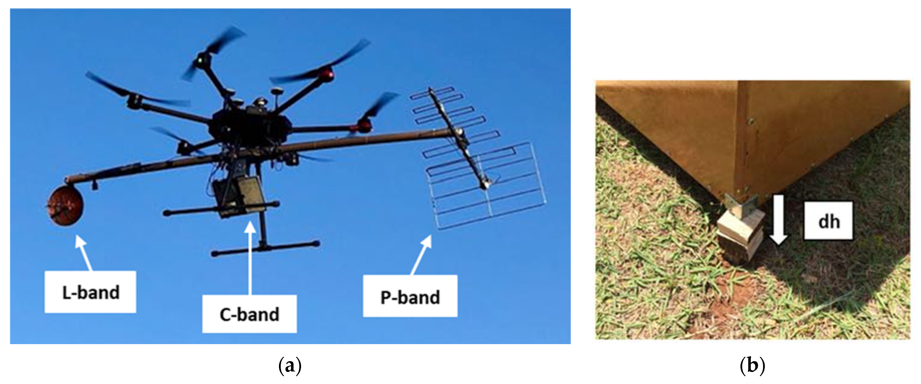
• The three corner reflectors were positioned at the UNICAMP test site at different radar incidence angles, between 36 and 60 degrees, as shown in Figure 2. Corner reflector 1, in the nearest range, had an incidence angle of 36 degrees. Corner reflector 2, in the middle range between 1 and 3, had an incidence angle of 52 degrees. Corner reflector 3, in far range, had an incidence angle of 60 degrees. Corner 2 was lifted differently during the second and third flights to validate the displacement measurement methodology.
• During the first flight, all three corner reflectors were placed horizontally on the ground, looking north.
• During the second flight, only the corner reflector number 2 was lifted 4 cm off the ground, as shown in Figure 1b. Corner reflectors 1 and 3 remained at ground level.
• During the third flight, only the corner reflector number 2 was lifted 2 cm off the ground. Corner reflectors 1 and 3 were still at ground level.
• The GNSS ground station and the drone were dismounted. The acquired data were downloaded for processing.

After the three flights, the data were processed as follows:

• Perform the differential GNSS processing of ground station and radar GNSS receivers.
• Generate position and antennae orientation history with IMU and differential GNSS data fusion.
• Process the raw radar data for each of the three flight paths mentioned above (raw data 1, 2, and 3) according to the processing chain described in [10] and shown in Figure 3: range and azimuth compression with motion compensation; recording of the three resulting single-look complex (SLC) images; interferometry (SLC 1 with SLC 2, generating the interferogram 1 and 2, and SLC 1 with SLC 3, producing the interferogram 1 and 3); topography subtraction and phase to height conversion; and complex filtering. The output consists of two deformation maps, plus the three SLCs, all in slant range geometry. Each interferogram is calculated from the SLCs with 0.1-m resolution in azimuth and 1 m resolution in the slant range. Complex filtering results on a final spatial resolution of 3 m in both slant range and azimuth directions for each deformation map.
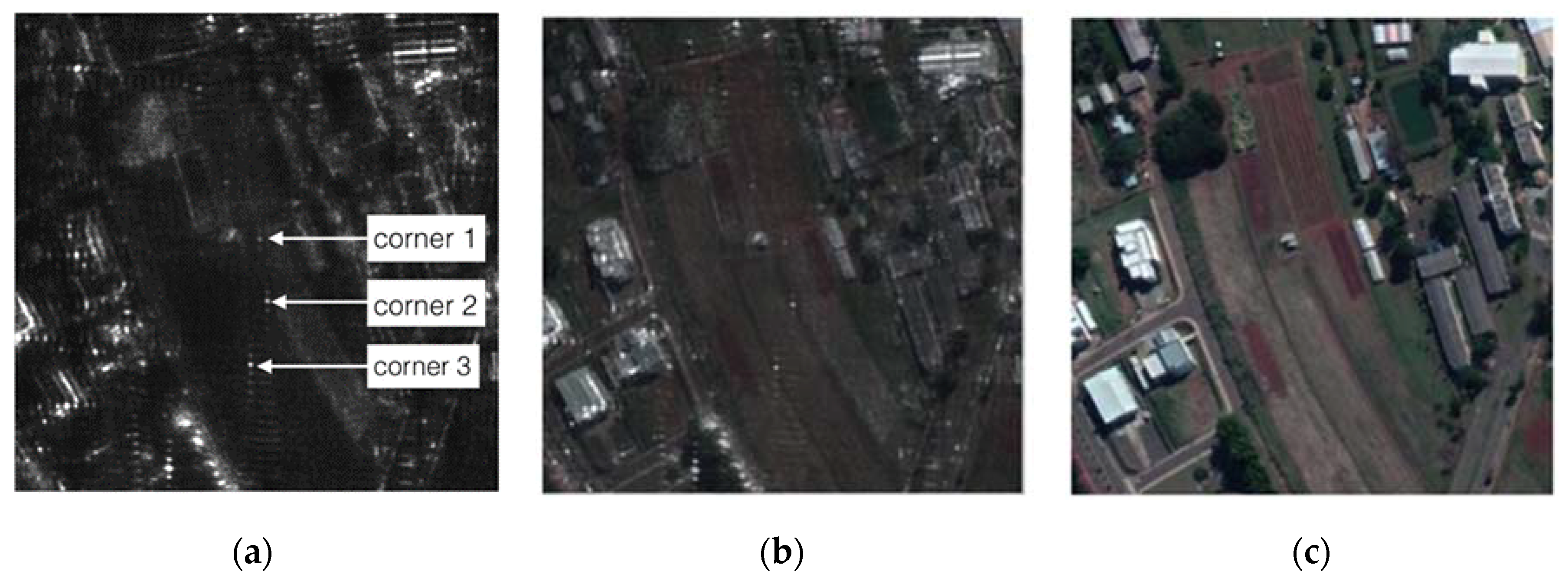
• Check the absolute position of the corner reflectors by searching their maximum power positions on the three slant range SLC images.
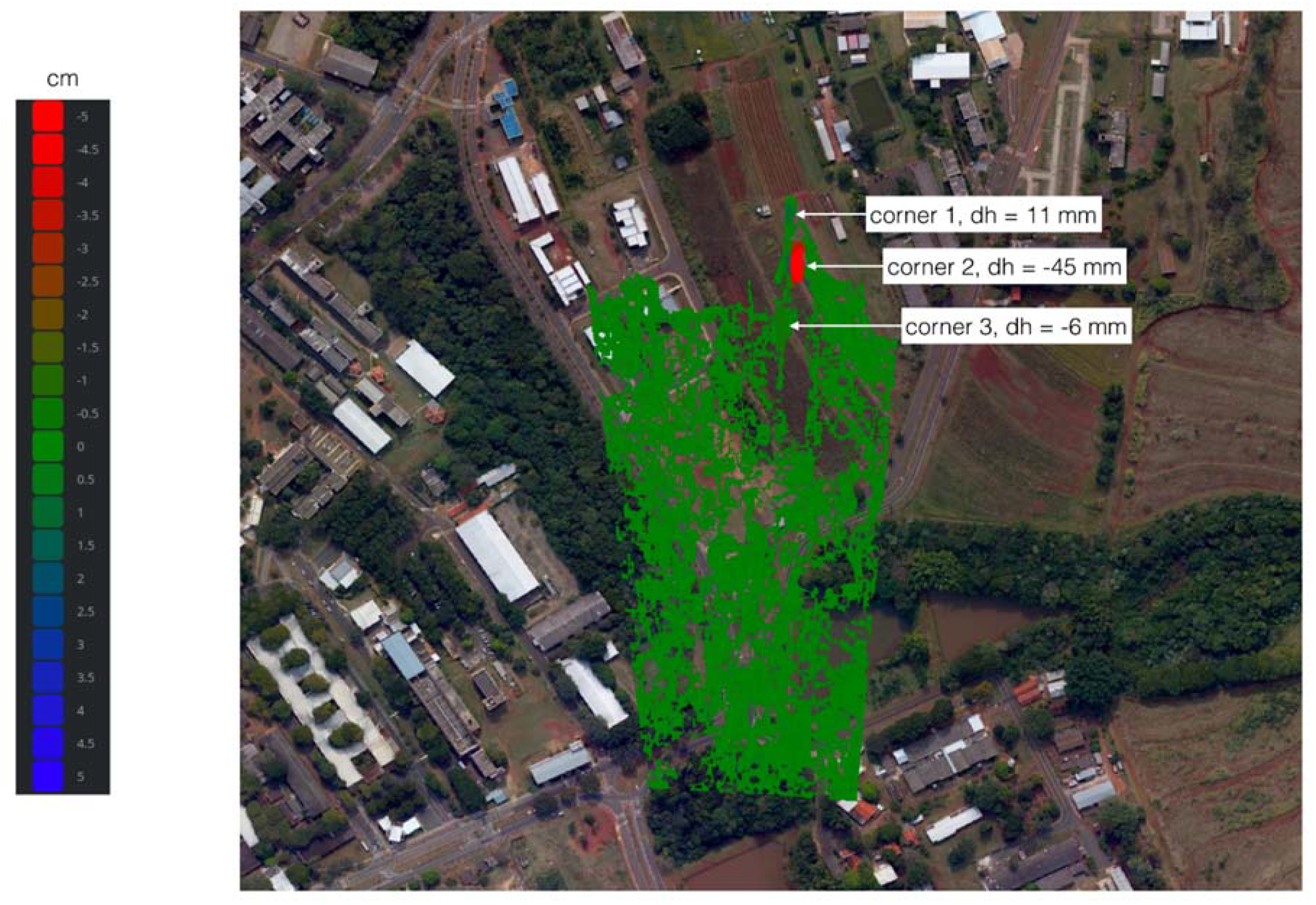
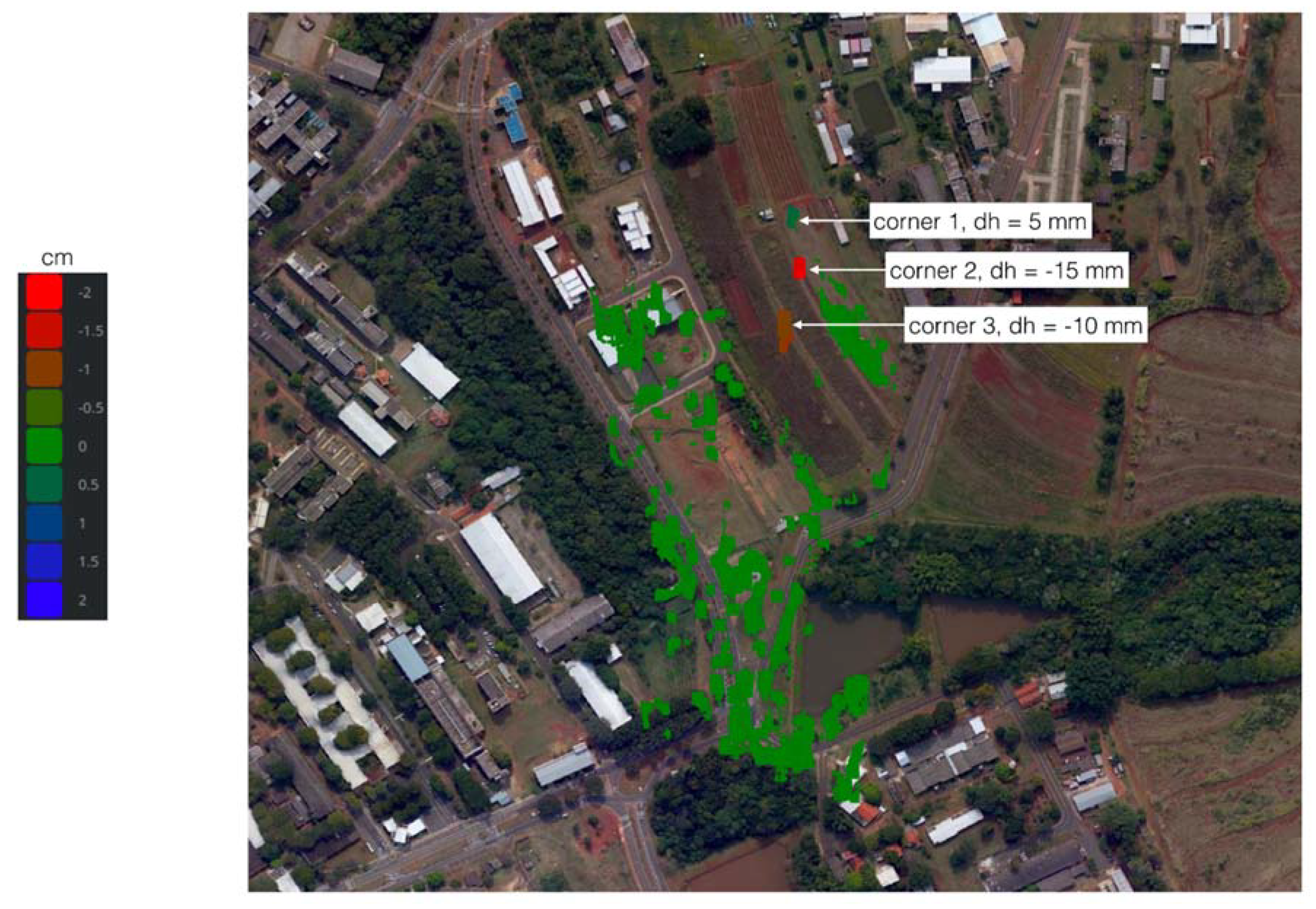
• Use the azimuth and slant range coordinates found in step 4 to read the displacement for each corner reflector on the deformation maps. Compare the displacement with the expected results:
  • Null differential height offsets for corner reflectors 1 and 3 on both deformation maps, since they were always at ground level;
  • A 4 cm lift for corner reflector 2 on the deformation map of interferogram 1 and 2;
  • A 2 cm lift for corner reflector 2 on the deformation map of interferogram 1 and 3.
• Geocode the two deformation maps.
• Generate the multi-look images from the SLCs with 1 m × 1 m resolution in slant range and geocode them, as shown in Figure 2a.

The chosen processing chain [10] was originally applied to an airborne DInSAR experiment. Nevertheless, it can be extended to this case thanks to the stability of the drone, which will be addressed in the next section. In particular, azimuth compression can be done at Zero Doppler, and motion compensation algorithms can be as effective as in the case of airborne DInSAR. The processing algorithm described in [12] was not used for this experiment because, unlike the processing chain reported in [10], it does not consider the topography subtraction step and does not deal with residual motion errors, which cause phase errors in the slant range SLC images.

3. Results

The drone performed three stable flights presenting an orientation error of less than 1-degree RMS and a position error of less than 0.2 m RMS. This behavior represented the majority of the research flights and was a positive surprise: well-stabilized hexacopter drones can repeat the same track within a 50 cm diameter tube and can hold the heading very close to the course direction. Figure 4 presents the deformation map derived from the first and the second flights, and Figure 5 shows the deformation map derived from the first and the third flights. Both Figure 4 and Figure 5 are geocoded and overlaid on an optical image. The displacement was measured according to steps 4 and 5 of the last section.

Table 3. Results overview of the two deformation maps.

Corner Reflectors	Deformation Map of 1 and 2 [mm]			Deformation Map 1 and 3 [mm]
	Ideal	Measured	Difference	Ideal	Measured	Difference
1	0	11	11	0	5	5
2	−40	−45	−5	−20	−15	5
3	0	−6	−6	0	−10	−10

shows the results overview of the two deformation maps. The displacement measurement error range is about 10 mm. The overall standard deviation of the displacement measurement is 7.4 mm, calculated with the six height difference values from the three corner reflectors and both deformation maps. It is six times better than the 45 mm error reported in [12]. Also, surfaces with a coherence better than 0.6, excluding the area of the corner reflector 2, show a standard deviation between 4 and 6 mm, as presented in

Table 4. Deformation map error overview, considering both deformation maps—right column: standard deviation of the deformation map error.

Targets	Standard Deviation [mm]
Corner Reflectors	7.4
Areas with Coherence Better than 0.6	4–6

.

The analysis of the results aforementioned is structured in the following five aspects mentioned in Section 1:

• signal-to-noise ratio;
• time decorrelation between the revisits;
• radar and processing phase stability;
• antennae environment;
• motion data.

3.1. Signal-to-Noise Ratio

The measured signal-to-noise ratio (SNR) of the corner reflectors is 32 dB, and their reflectivity is 20 dB. The SNR and the reflectivity of the surrounding grass area are 7 dB and −5 dB, respectively. The SNR of the neighboring bare soil is 3 dB, and the reflectivity is −9 dB, as shown in

Table 5. DInSAR parameters calculated considering the reflectivity and signal-to-noise ratio (SNR) of the corner reflector and the grass surface.

Targets	Reflectivity [dB]	SNR [dB]	Coherence [0–1]	Unfiltered Phase Noise [deg.]	Filtered Phase Noise [deg.]	Standard Deviation of the Displacement Measurement Error [mm]
Corner reflectors	20	32	~1	4	0.4	0.13
Grass	−5	7	0.8	52	5.2	1.6
Bare soil	−9	3	0.6	70	7	2.2

. The expected coherence, the unfiltered interferometric phase noise, the filtered phase noise, and the standard deviation of the displacement error are calculated according to [13]. This standard deviation is caused exclusively by the SNR. The filtered phase has a resolution of 3 m by 3 m, starting from the unfiltered phase with 1 m resolution in range and 0.1-m resolution in azimuth. The resulting standard deviation of the displacement measurement error is 0.13 mm for the corner reflectors, 1.6 mm for the grass or distributed targets with an average reflectivity of −5 dB, and 2.2 mm for bare soil or distributed targets with an average reflectivity of −9 dB.

3.2. Time Decorrelation Between the Revisits

As the radar operates in the L-band, the decorrelation within a day is negligible [7]. The high coherence of the interferograms 1 and 2 and 1 and 3 also shows that the contribution of hours of the revisit time does not have any influence on the degradation of the deformation map accuracy. The measured coherence is compatible with the measured SNR and does not contribute the time decorrelation.

3.3. Radar and Processing Phase Stability

The phase errors caused by the radar and the processing chain are less than 1 degree. The resulting error has a standard deviation at the deformation map of less than 0.4 mm.

3.4. Antennae Environment

Airborne SAR systems have considerable phase errors caused by secondary reflections of the pulse transmission and backscatter signal reflections at the fuselage and wings. Thus, several corrections and considerations are required. Fortunately, this was not a great issue for the drone-borne DInSAR system, shown in Figure 1a, since the influence of the class 3 drone on the radar was negligible. No changes in the antenna diagram, no variation in the antenna gain, and no secondary reflections were observed.

3.5. Motion Data

Considering Table 2, the major contribution for the MSS error is from the differential GNSS calculation as the orientation errors are negligible due to the small lever arms between the MSS and the L-band antenna. For the DInSAR, only the relative position accuracy is relevant, as the absolute position error can be compensated by taking a ground reference target. A precise differential GNSS calculation with a fixed phase solution was obtained because the ground station was always closer than 2 km to the drone, and the integration time before and after each flight was greater than 10 min. The IMU/D-GNSS fusion program delivers only a rough estimation of the relative position accuracy. Here, a relative position accuracy was estimated at 5 mm.

4. Discussion

Table 6. Error source budget of the deformation map. There are five sources and a total measured error of about 4–7.4 mm.

Error Sources	Standard Deviation [mm]
SNR	<2.2
Time Decorrelation	~0
Radar and Processing Phase Stability	<0.4
Antenna Environment	~0
Motion Data	~5
Total Measured RMS Error	4–7.4

presents an overview of the deformation map error sources. The total measured error corresponds to the geometric average of all five contributions mentioned in Section 3.1, Section 3.2, Section 3.3, Section 3.4 and Section 3.5, as all these sources are statistically uncorrelated. The error contributions from SNR, time decorrelation, radar and processing phase stability, and antenna environment can be neglected when compared to the motion data error contribution. The MSS processing error, estimated at 5 mm, is by far the main source of error for the deformation map accuracy since it is approximately equal to the total deformation map error of about 4–7.4 mm. Regarding the SNR, the breakdown of Table 5 shows that all three target types—the corner reflectors and the grass and bare soil areas—contribute less than the motion data error to the total measured error. Both distributed and point targets have the same relation between coherence and phase noise in the interferogram, due to the short revisit time that causes a negligible time decorrelation.

The coherence thresholds of Figure 4 and Figure 5 are 0.6 and 0.75, respectively. If both deformation maps had the same threshold value, the two figures would be nearly identical, except for the area related to corner reflector 2. A comparison between them shows that the most appropriate coherence threshold for these interferograms is 0.6 since the use of 0.75 would discard much useful information. This is why all the quantitative results were presented for a coherence threshold of 0.6.

5. Conclusions

The drone-borne DInSAR system introduced in [12] was operated to perform the experiment presented in this work and was able to generate deformation maps with 4–7.4 mm accuracy. Ground deformation maps with such high accuracy are valuable for monitoring areas and constructions in early warning and emergency management systems for disaster mitigation. Furthermore, the easy transportability of the drone-borne DInSAR system can allow quick and low-cost monitoring of small areas like dams and mining sites.

An overview of the accuracy assessments of deformation maps can be summarized as follows.

• The accuracy assessment in L-band presented here is, as far as we know, novel;
• C- and X-band satellite-borne systems reported in [14,15,16] and the airborne system published in [10] have similar accuracy.

The achievement of a high and stable deformation map accuracy with only two flight tracks and with low time decorrelation effects reported here is, to the best of our knowledge, unique.

In future works, multiple frequency differential GNSS shall improve accuracy. However, the improvement will not be very significant as the range between the GNSS ground station and the drone will always be less than a few kilometers. Additionally, P- and C-bands deformation maps shall be explored and merged with the L-band one. A three-band deformation map will have improved accuracy and a decorrelation time of several years due to the P-band [9]. Additionally, we have been working with the time-domain back-projection algorithm and expect to publish DInSAR results in the near future.

References

1. Gabriel, A.K.; Goldstein, R.M.; Zebker, H.A. Mapping small elevation changes over large areas: Differential radar interferometry. J. Geophys. Res. 1989, 94, 9183. [Google Scholar] [CrossRef]
2. Prats-Iraola, P.; Lopez-Dekker, P.; De Zan, F.; Yagüe-Martínez, N.; Zonno, M.; Rodriguez-Cassola, M. Performance of 3-D surface deformation estimation for simultaneous squinted SAR acquisitions. IEEE Trans. Geosci. Remote Sens. 2018, 56, 2147–2158. [Google Scholar] [CrossRef] [Green Version]
3. Jung, H.; Lu, Z.; Sherhperd, A.; Wright, T. Simulation of the superSAR multi-azimuth Synthetic Aperture Radar imaging system for precise measurement of three-dimensional earth surface displacement. IEEE Trans. Geosci. Remote Sens. 2015, 53, 6196–6206. [Google Scholar] [CrossRef]
4. Kimura, H. Three-dimensional surface deformation mapping from multi-directional SAR interferograms. In Proceedings of the 2017 IEEE International Geoscience and Remote Sensing Symposium (IGARSS), Fort Worth, TX, USA, 23–28 July 2017; pp. 1692–1695. [Google Scholar]
5. Jo, M.; Jung, H.; Won, J.; Poland, M.P.; Miklius, A. Measurement of three-dimensional surface deformation of the March 2011 Kamoamoa fissure eruption, Kilauea Volcano, Hawai’i. In Proceedings of the 2014 IEEE Geoscience and Remote Sensing Symposium (IGARSS), Quebec City, QC, Canada, 13–18 July 2014; pp. 437–440. [Google Scholar]
6. Jung, H.; Yung, S.; Jo, M. An improvement of Multiple-Aperture SAR interferometry performance in the presence of complex and large line-of-sight deformation. IEEE J. Sel. Top. Appl. Earth Obs. Remote Sens. 2015, 8, 1743–1752. [Google Scholar] [CrossRef]
7. Reigber, A.; Scheiber, R. Airborne differential SAR interferometry: First results at L-band. IEEE Trans. Geosci. Remote Sens. 2003, 41, 1516–1520. [Google Scholar] [CrossRef]
8. Fornaro, G.; Lanari, R.; Sansosti, E.; Franceschetti, G.; Perna, S.; Gois, A.; Moreira, J. Airborne differential interferometry: X-band experiments. In Proceedings of the 2004 IEEE International Geoscience and Remote Sensing Symposium (IGARSS), Anchorage, AK, USA, 20‒24 September 2004; Volume 5, pp. 3329–3332. [Google Scholar]
9. De Macedo, K.A.C.; Wimmer, C.; Barreto, T.L.M.; Lübeck, D.; Moreira, J.R.; Rabaco, L.M.L.; de Oliveira, W.J. Long-term airborne DInSAR measurements: P- and X-band cases. In Proceedings of the 2011 IEEE International Geoscience and Remote Sensing Symposium (IGARSS), Vancouver, BC, Canada, 24‒29 July 2011; pp. 1175–1178. [Google Scholar]
10. Perna, S.; Wimmer, C. X-Band Airborne Differential Interferometry: Results of the OrbiSAR Campaign Over the Perugia Area. IEEE Trans. Geosci. Remote Sens. 2008, 46, 489–503. [Google Scholar] [CrossRef]
11. Cao, N.; Lee, H.; Zaugg, E.; Shrestha, R.; Carter, W.; Glennie, C.; Wang, G.; Lu, Z.; Fernandez-Diaz, J.C. Airborne DInSAR Results Using Time-Domain Backprojection Algorithm: A Case Study Over the Slumgullion Landslide in Colorado With Validation Using Spaceborne SAR, Airborne LiDAR, and Ground-Based Observations. IEEE J. Sel. Top. Appl. Earth Obs. Remote Sens. 2017, 10, 4987–5000. [Google Scholar] [CrossRef]
12. Moreira, L.; Castro, F.; Góes, J.A.; Bins, L.; Teruel, B.; Fracarolli, J.; Castro, V.; Alcântara, M.; Oré, G.; Luebeck, D.; et al. A Drone-borne Multiband DInSAR: Results and Applications. In Proceedings of the 2019 IEEE Radar Conference (RadarConf), Boston, MA, USA, 22‒26 April 2019; pp. 1–6. [Google Scholar]
13. Just, D.; Bamler, R. Phase statistics of interferograms with applications to synthetic aperture radar. Appl. Opt. 1994, 33, 4361. [Google Scholar] [CrossRef] [PubMed]
14. Casu, F.; Manzo, M.; Lanari, R. A quantitative assessment of the SBAS algorithm performance for surface deformation retrieval from DInSAR data. Remote Sens. Env. 2006, 102, 195–210. [Google Scholar] [CrossRef]
15. Bonano, M.; Manunta, M.; Pepe, A.; Paglia, L.; Lanari, R. From Previous C-Band to New X-Band SAR Systems: Assessment of the DInSAR Mapping Improvement for Deformation Time-Series Retrieval in Urban Areas. IEEE Trans. Geosci. Remote Sens. 2013, 51, 1973–1984. [Google Scholar] [CrossRef]
16. Manunta, M.; De Luca, C.; Zinno, I.; Casu, F.; Manzo, M.; Bonano, M.; Fusco, A.; Pepe, A.; Onorato, G.; Berardino, P.; et al. The Parallel SBAS Approach for Sentinel-1 Interferometric Wide Swath Deformation Time-Series Generation: Algorithm Description and Products Quality Assessment. IEEE Trans. Geosci. Remote Sens. 2019, 57, 6259–6281. [Google Scholar] [CrossRef]
Figure 1. Experiment components. (a) Drone-borne differential synthetic aperture radar interferometry (DInSAR) system [12] including one L-band antenna with H and V dipoles; two interferometric C-band antennae attached to the radar electronics; one P-band antenna with an H dipole. (b) Corner reflector 2, which was lifted 4 cm off the ground during the second flight and 2 cm during the third flight. Displacement is positive (dh > 0) when terrain height decreases with time.
Remotesensing 12 00778 g001
Figure 2. Test area at UNICAMP, Campinas Brazil. (a) Geocoded L-band SAR image of the first flight, with the indication of the position of the three corner reflectors: corner 1 in the nearest range, corner 2 in the middle range, and corner 3 in the far range. Flight track on the top of the image, from west to east (left to right), looking south (downward). (b) Overlay of SAR and optical images to show the target’s position. (c) Optical image taken on the same day.
Remotesensing 12 00778 g002
Figure 3. Simplified flow chart of the processing chain. The complete version is in [10]. I 12 is the interferogram 1 and 2, and I 13 is the interferogram 1 and 3.
Remotesensing 12 00778 g003
Figure 4. Deformation map of the interferogram 1 and 2—from the first and the second flights. Displacement is positive (dh > 0) when terrain height decreases with time. The coherence threshold is 0.6. Corner reflector 2 was lifted 4 cm in the second flight. The measured displacement was −45 mm.
Remotesensing 12 00778 g004
Figure 5. Deformation map of the interferogram 1 and 3—from the first and the third flights. Displacement is positive (dh > 0) when terrain height decreases with time. The coherence threshold is 0.75. Corner reflector 2 was lifted 2 cm in the second flight. The measured displacement was −15 mm.
Remotesensing 12 00778 g005