An End-to-End and Localized Post-Processing Method for Correcting High-Resolution Remote Sensing Classification Result Images

1
School of Computer Technology and Engineering, Changchun Institute of Technology, Changchun 130012, China
2
Jilin Provincial Key Laboratory of Changbai Historical Culture and VR Reconstruction Technology, Changchun Institute of Technology, Changchun 130012, China
*
Author to whom correspondence should be addressed.
Remote Sens. 2020, 12(5), 852; https://0-doi-org.brum.beds.ac.uk/10.3390/rs12050852
Submission received: 7 February 2020
/
Revised: 4 March 2020
/
Accepted: 5 March 2020
/
Published: 6 March 2020
(This article belongs to the Special Issue Advanced Deep Learning Strategies for the Analysis of Remote Sensing Images)
Abstract
:Since the result images obtained by deep semantic segmentation neural networks are usually not perfect, especially at object borders, the conditional random field (CRF) method is frequently utilized in the result post-processing stage to obtain the corrected classification result image. The CRF method has achieved many successes in the field of computer vision, but when it is applied to remote sensing images, overcorrection phenomena may occur. This paper proposes an end-to-end and localized post-processing method (ELP) to correct the result images of high-resolution remote sensing image classification methods. ELP has two advantages. (1) End-to-end evaluation: ELP can identify which locations of the result image are highly suspected of having errors without requiring samples. This characteristic allows ELP to be adapted to an end-to-end classification process. (2) Localization: Based on the suspect areas, ELP limits the CRF analysis and update area to a small range and controls the iteration termination condition. This characteristic avoids the overcorrections caused by the global processing of the CRF. In the experiments, ELP is used to correct the classification results obtained by various deep semantic segmentation neural networks. Compared with traditional methods, the proposed method more effectively corrects the classification result and improves classification accuracy.
1. Introduction
With the advent of high-resolution satellites and drone technologies, an increasing number of high-resolution remote sensing images have become available, making automated processing technology increasingly important for utilizing these images effectively [1]. High-resolution remote sensing image classification methods, which automatically provide category labels for objects in these images, are playing an increasingly important role in land resource management, urban planning, precision agriculture, and environmental protection [2]. However, high-resolution remote sensing images usually contain detailed information and exhibit high intra-class heterogeneity and inter-class homogeneity characteristics, which are challenging for traditional shallow-model classification algorithms [3]. To improve classification ability, deep learning technology, which can extract higher-level features in complex data, has been widely studied in the high-resolution remote sensing classification field in recent years [4].
Deep semantic segmentation neural networks (DSSNNs) are constructed based on convolutional neural networks (CNNs); the input of these models is an image patch, and the output are category labels for the image patch. With the help of this structure, a DSSNN gains the ability to perform rapid pixel-wise classification and end-to-end data processing—characteristics that are critical in automatically analyzing remote sensing images [5,6]. In the field of remote sensing classification, the most widely used DSSNN architectures include fully convolutional networks (FCNs), SegNETs, and U-Nets [7,8,9]. Many studies have extended these architectures by adding new neural connection structures to address different remote sensing object recognition tasks [10]. In the process of segmenting high-resolution remote sensing images of urban buildings, due to their hierarchical feature extraction structures, DSSNNs can extract buildings’ spatial and spectral building features and achieve better building recognition results [11,12]. When applied to road extraction from images, DSSNNs can integrate low-level features into higher-level features layer by layer and extract the relevant features [13,14]. Based on U-Nets, FCNs, and transmitting structures that add additional spatial information, DSSNNs can improve road border and centerline recognition accuracy obtained from high-resolution remote sensing images [15]. Through the FCN and SegNET architectures, DSSNNs can obtain deep information regarding land cover areas and can classify complex land cover systems in an automatic and end-to-end manner [16,17,18].
In many high-resolution remote sensing semantic segmentation application tasks, obtaining accurate object boundaries is crucial [19,20]. However, due to the hierarchical structures of DSSNNs, some object spatial information may be lost during the training and classification process; consequently, their classification results are usually not perfect, especially at object boundaries [21,22]. Conditional random field (CRF) methods are widely used to correct segmentation or super-pixel classification results [23,24]. CRFs can also be integrated into the training stage to enhance a CNN’s classification ability [25,26]. Due to their ability to capture fine edge details, CRFs are also useful for post-processing the results of remote sensing classification [27]. Using CRFs, remote sensing image semantic segmentation results can be corrected, especially at ground object borders [28,29,30]. Although CRFs have achieved many successes in the field of computer vision, when applied to remote sensing images where the numbers, sizes, and locations of objects vary greatly, some of the ground objects will be excessively enlarged or reduced and shadowed areas may be confused with adjacent objects [31]. To address the above problem, training samples or contexts can be introduced to restrict the behavior of CRFs, limiting their processes within a certain range, category, or number of iterations [32,33]. Unfortunately, these methods require the introduction of samples to the CRF control process, and these samples cause the corresponding methods to lose their end-to-end characteristics. For classification tasks based on deep semantic segmentation networks, when the end-to-end characteristics are lost, the classification work must add an additional manual sample set selection and construction process, which reduces the ability to apply semantic segmentation to networks automatically and decreases their application value [34]. Therefore, new methods must be introduced to solve this problem.
To address the above problems, this paper proposes an end-to-end and localized post-processing method (ELP) for correcting high-resolution remote sensing image classification results. By introducing a mechanism for end-to-end evaluation and a localization procedure, ELP can identify which locations of the resulting image are highly suspected to have errors without requiring training and verification samples; then, it can apply further controls to restrict the CRF analysis and update areas within a small range and limit the iteration process. In the experiments, we introduce study images from the “semantic labeling contest of the ISPRS WG III/4 dataset” and apply various DSSNNs to obtain classification result images. The results show that compared with the traditional CRF method, the proposed method more effectively corrects classification result images and improves classification accuracy.
2. Methodology
2.1. Deep Semantic Segmentation Neural Networks’ Classification Strategy and Post-Processing
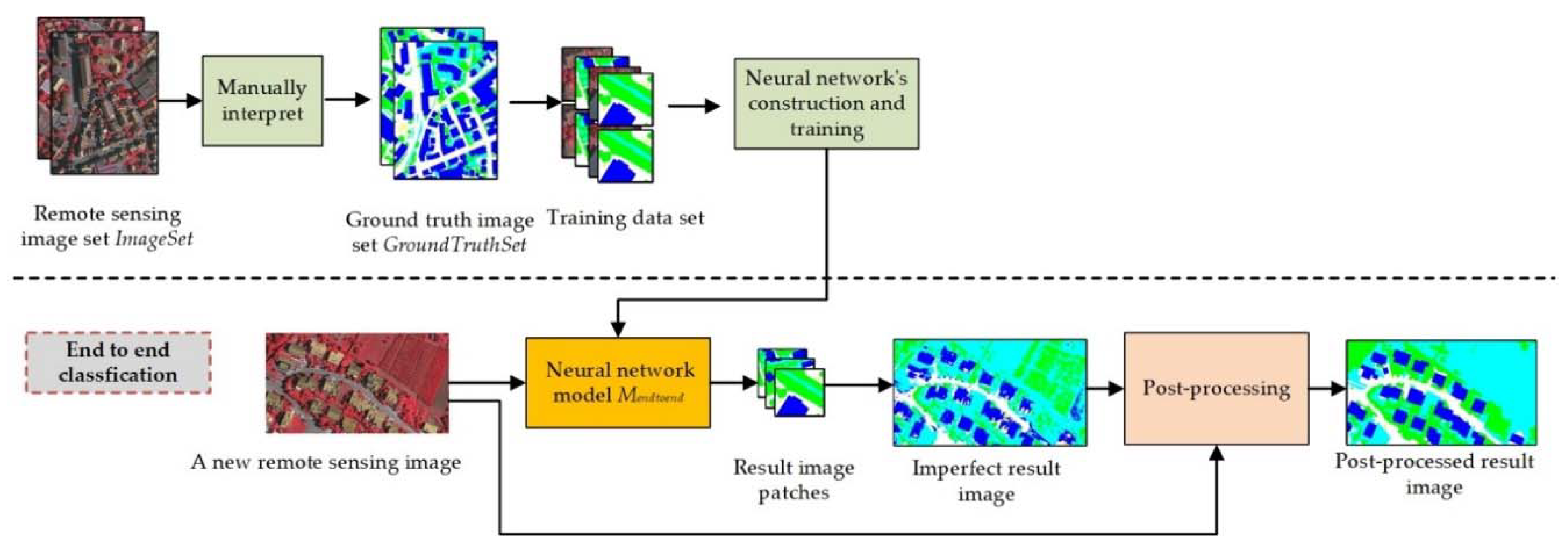
Deep semantic segmentation neural networks such as FCNs, SegNET, and U-NET have been widely studied and applied by the remote sensing image classification research community. The training and classification processes of these networks are illustrated in Figure 1.
As shown in Figure 1, the end-to-end classification strategy is usually adopted for DSSNNs’ training and classification. During the training stage, a set of remote sensing images ImageSet = {I1, I2, …, In} is adopted and manually interpreted into a ground truth set GroundTruthSet = {Igt1, Igt2, …, Igtn}; then, the GroundTruthSet is separated into patches to construct the training dataset. The classification model Mendtoend is obtained based on this training dataset. During the classification stage, the classification model is utilized to classify a completely new remote sensing image Inew (not an image from ImageSet). This strategy achieves a higher degree of automation; the classification process has no relationship with the training data or the training algorithm, and newly obtained or other images in the same area can be classified automatically with Mendtoend, forming an input-to-output/end-to-end structure. Thus, this strategy is more valuable in practical applications when massive amounts of remote sensing data need to be processed quickly.
However, the classification results of the end-to-end classification strategy are usually not "perfect", and they are affected by two factors. On the one hand, because the training data are constructed by manual interpretation, it is difficult to provide training ground truth images that are precise at the pixel level (especially at the boundaries of ground objects). Moreover, the incorrectly interpreted areas of these images may even be amplified through the repetitive training process [16]. On the other hand, during data transfer among the neural network layers, along with obtaining high-level spatial features, some spatial context information may be lost [35]. Therefore, the classification results obtained by the "end-to-end classification strategy" may result in many flaws, especially at ground object boundaries. To correct these flaws, in the computer vision research field, the conditional random field (CRF) method is usually adopted in the post-processing stage to correct the result image. The conditional random field can be defined as follows:
where F is a set of random variables {F1, F2, …, FN}; Fi is a pixel vector; X is a set of random variables {x1, x2, …, xN}, where xi is the category label of pixel i; Z(F) is a normalizing factor; and c is a clique in a set of cliques Cg, where g induces a potential φc [23,24]. By calculating Equation (1), the CRF adjusts the category label of each pixel and achieves the goal of correcting the result image. The CRF is highly effective at processing images that contain only a small number of objects. However, the numbers, sizes, and locations of objects in remote sensing images vary widely, and the traditional CRF tends to perform a global optimization of the entire image. This process leads to some ground objects being excessively enlarged or reduced. Furthermore, if the different parts of ground objects that are shadowed or not shadowed are processed in the same manner, the CRF result will contain more errors [31]. In our previous work, we proposed a method called the restricted conditional random field (RCRF) that can handle the above situation [31]. Unfortunately, the RCRF requires the introduction of samples to control its iteration termination and produce an output integrated image. When integrated into the classification process, the need for samples will cause the whole classification process to lose its end-to-end characteristic; thus, the RCRF cannot be integrated into an end-to-end process. In summary, to address the above problems, the traditional CRF method needs to be further improved by adding the following characteristics:
(1) End-to end result image evaluation: Without requiring samples, the method should be able to automatically identify which areas of a classification result image may contain errors. By identifying areas that are strongly suspected of being misclassified, we can limit the CRF process and analysis scope.
(2) Localized post-processing: The method should be able to transform the entire image post-processing operation into local corrections and separate the various objects or different parts of objects (such as roads in shadow or not in shadow) into sub-images to alleviate the negative impacts of differences in the number, size, location, and brightness of objects.
To achieve this goal, a new mechanism must be introduced to improve the traditional CRF algorithm for remote sensing classification results post-processing.
2.2. End-to-End Result Image Evaluation and Localized Post-Processing
The majority of evaluation methods for classification results require samples with category labels that allow the algorithm to determine whether the classification result is good; however, to achieve an end-to-end classification results evaluation, samples cannot be required during the evaluation process. In the absence of testing samples, although it is impossible to accurately indicate which pixels are incorrectly classified, we can still find some areas that are highly suspected of having classification errors by applying some conditions.
Therefore, we need to establish a relation between the remote sensing image and the classification result image and find the areas where the colors (bands) of the remote sensing image are consistent, but the classification results are inconsistent; these are the areas that may belong to the same object but are incorrectly classified into different categories. Such areas are strong candidates for containing incorrectly classified pixels. Furthermore, we try to correct these errors within a relatively small area.
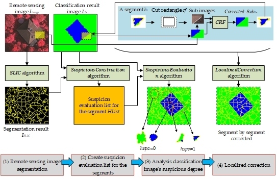
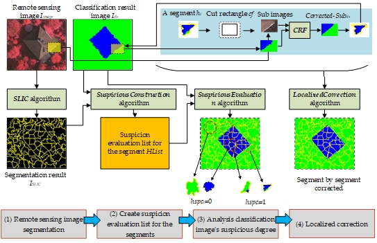
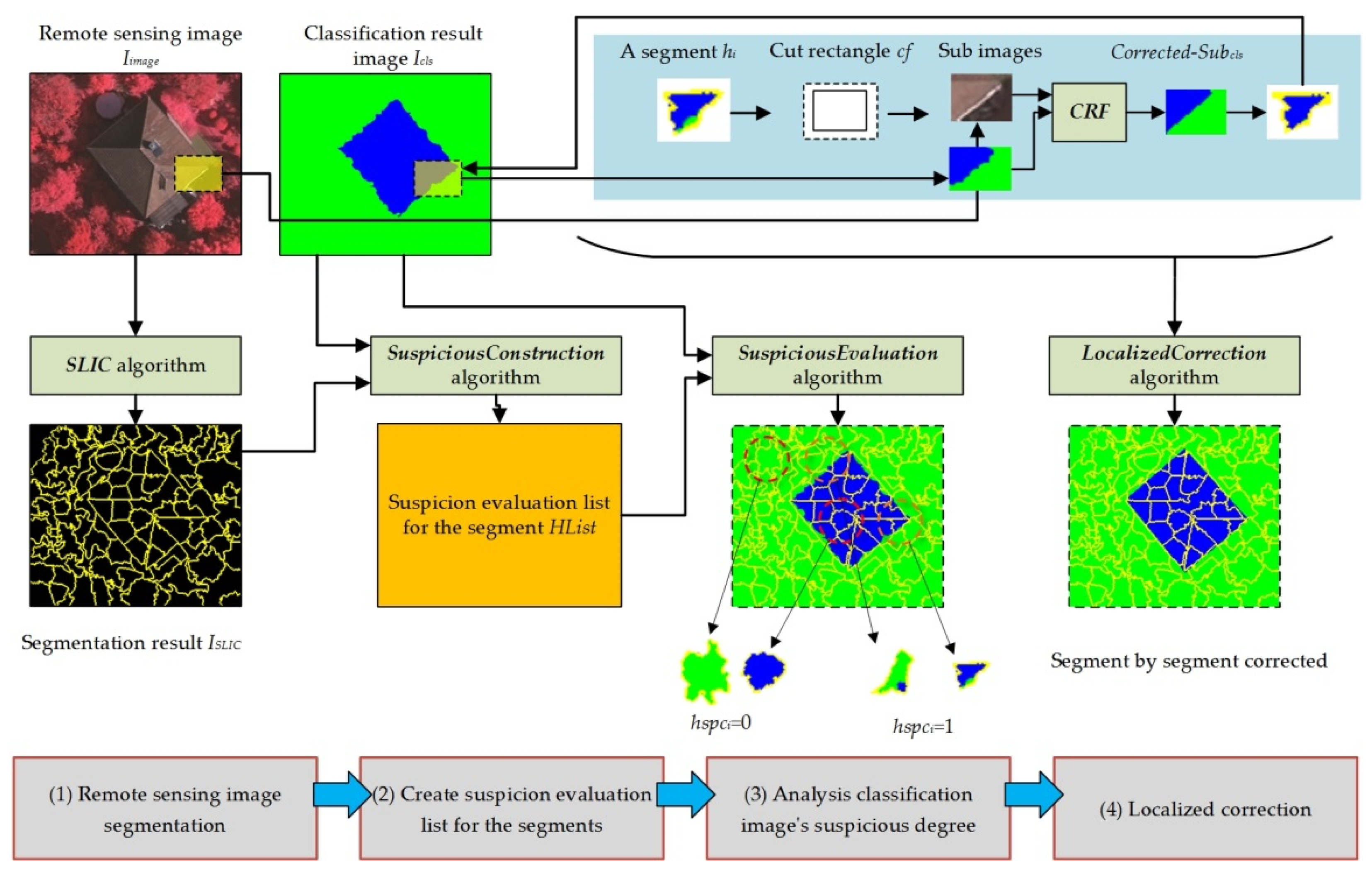
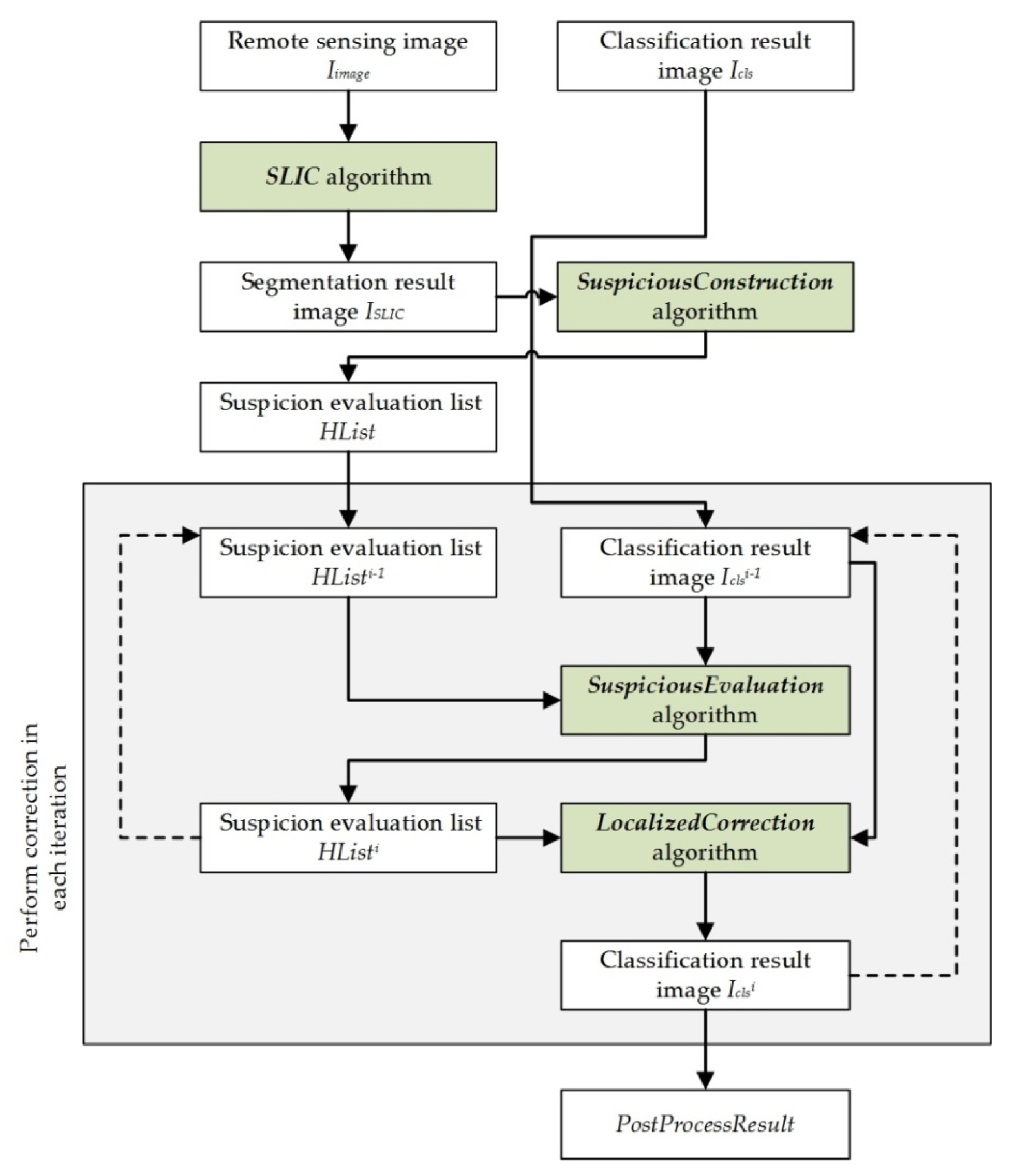
To achieve the above goals, for a remote sensing image Iimage and its corresponding classification image Icls, the methods proposed in this paper are illustrated in Figure 2:
As shown in Figure 2, we use four steps to perform localized correction:
(1) Remote sensing image segmentation
We need to segment the remote image based on color (band value) consistency. In this paper, we adopt the simple linear iterative clustering (SLIC) algorithm as the segmentation method. The algorithm initially contains k clusters. Each cluster is denoted by Ci = {li, ai, bi, xi, yi}, where li, ai, and bi are the color values of Ci in CIELAB color space, and xi, yi are the center coordinates of Ci in the image. For two clusters, Ci and Cj, the SLIC algorithm is introduced to compare color and space distances simultaneously, as follows:
where distancecolor is the color distance and distancespace is the spatial distance. Based on these two distances, the distance between the two clusters is:
where Ncolor is the maximum color distance and Nspace is the maximum position distance. The SLIC algorithm uses the iterative mechanism of the k-means algorithm to gradually adjust the cluster position and the cluster to which each pixel belongs, eventually obtaining Nsegment segments [36]. The advantage of the SLIC algorithm is that it can quickly and easily cluster adjacent similar regions into a segment; this characteristic is particularly useful for finding adjacent areas that have a consistent color (band value). For Iimage, the SLIC algorithm is used to obtain the segmentation result ISLIC. In each segment in ISLIC, the pixels are assigned the same segment label.
(2) Create a list of segments with suspicious degree evaluations
For all the segments in ISLIC, a suspicion evaluation list for the segments HList = {h1, h2, …, hn} is constructed, where hi is a set hi = {hidi, hpixelsi, hreci, hspci}, hidi is a segment label, hpixelsi holds the locations of all the pixels in the segment; hreci is the location and size of the enclosing frame rectangle of hpixelsi; and hspci is a suspicious evaluation value, which is either 0 or 1—a “1” means that the pixels in the segment are suspected of being misclassified, and a “0” means that the pixels in the segment are likely correctly classified. The algorithm to construct the suspicious degree evaluation list is as follows (SuspiciousConstruction Algorithm):
| Algorithm SuspiciousConstruction |
| Input:ISLIC |
| Output:HList |
| Begin |
| HList = an empty list; |
| foreach (segment label i in ISLIC){ |
| hidi = i; |
| hpixelsi = Locations of all the pixels in corresponding segment i; |
| hreci= the location and size of hpixelsi’s enclosing frame rectangle; |
| hspci = 0; |
| hi = Create a set {hidi, hpixelsi, hreci, hhypi}; |
| HList ← hi; |
| } |
| return HList; |
| End |
In the SuspiciousConstruction algorithm, by default, each segment’s spci = 0 (the hypothesis is that no misclassified pixels exist in the segment).
(3) Analyze the suspicious degree
As shown in Figure 2, for a segment, the spci value can be calculated based on the pixels in ISLIC; hi’s corresponding pixels can be grouped as SP = {sp1, sp2, …, spm}, where spi is the pixel number belonging to category i, and the inconsistency degree of SP can be described using the following formula:
Based on this formula, the value of hypi can be expressed as follows:
where α is a threshold value (the default is 0.05). When a segment’s hspci = 0, the segment’s corresponding pixels in ISLIC all belong to the same category, which indicates that pixels’ features are consistent in both Iimage (band value) and ISLIC (segment label); in this case, the segment does not need correction by CRF. In contrast, when a segment’s hspci = 1, the pixels of the segment in ISLIC belong to different categories, but the pixel’s color (band value) is comparatively consistent in Iimage; this case may be further subdivided into two situations:
A. Some type of classification error exists in the segment (such as the classification result deformation problem appearing on an object boundary).
B. The classification result is correct, but the segment crosses a boundary between objects in ISLIC (for example, the number of segments assigned to the SLIC algorithm is too small, and some areas are undersegmented).
In either case, we need to be suspicious of the corresponding segment and attempt to correct mistakes using CRF. Based on Formulas 5 and 6, the algorithm for analyzing Icls using HList is as follows (SuspiciousEvaluation Algorithm):
| Algorithm SuspiciousEvaluation |
| Input:HList, Icls |
| Output:HList |
| Begin |
| foreach(Item hi in HList){ |
| SP = new m-element array with zero values |
| foreach(Location pl in hi.hpixelsi){ |
| px = Obtain pixel at pl in Icls; |
| pxcl = Obtain category label of px; |
| SP[pxcl] = SP[pxcl] + 1; |
| } |
| inconsistence = Use Formula (5) to calculate SP; |
| hi.hypi = Use Formula (6) with inconsistence |
| } |
| return HList; |
| End |
By applying the SuspiciousEvaluation algorithm, we can identify which segments are suspicious and require further post-processing.
(4) Localized correction
As shown in Figure 2, for a segment hi that is suspected of containing error classified pixels, the post-processing strategy can be described as follows: First, based on hi.hreci, create a cut rectangle cf, (cf = rectangle hi.hreci enlarged by β pixels), where β is the number of pixels to enlarge and the default value is 10. Second, use the cf cut sub-images from Iimage and Icls to obtain a Subimage and a Subcls. Third, input Subimage and Subcls to the CRF algorithm, and obtain a corrected classification result Corrected-Subcls. Finally, based on the pixel locations in hi.hpixelsi, obtain the pixels from Corrected-Subcls and write them to Icls, which constitutes localized area correction on Icls. For the entire Icls, the localized correction algorithm on Icls is as follows (LocalizedCorrection Algorithm):
| Algorithm LocalizedCorrection |
| Input:Icls, HList |
| Output:Icls |
| Begin |
| foreach(hi in HList){ |
| if (hi.hspci==0) then continue; |
| cf= Enlarge rectangle hi.hreci by β pixels; |
| Subimage, Subcls = Cut sub-images from Iimage and Icls; |
| Corrected-Subcls = Process Subimage and Subcls by CRF algorithm; |
| pixels = Obtain pixels in hi.hpixelsi from Corrected-Subcls; |
| Icls←pixels; |
| } |
| return Icls |
| End |
By applying the LocalizedCorrection algorithm, the ICLS will be corrected segment by segment through the CRF algorithm.
2.3. Overall Process of the End-to-End and Localized Post-Processing Method
Based on the four steps and algorithms described in the preceding subsection, we can evaluate the classification result image without requiring testing samples and correct the classification result image within local areas. By integrating these algorithms, we propose an end-to-end and localized post-processing method (ELP) whose input is a remote sensing image Iimage and a classification result image Icls, and whose output is the corrected classification result image. Through the iterative and progressive correction process, the goal of improving the quality of the ICLS can be achieved. The process of ELP is shown in Figure 3.
As Figure 3 shows, the ELP method is a step-by-step iterative correction process that requires a total of γ iterations to correct the Icls content. Before beginning the iteration, the ELP method obtains the segmentation result image ISLIC before iteration:
Then, it evaluates the segments and constructs the suspicion evaluation list for the segments HList:
In each iteration, ELP updates HList to obtain HListη, and it outputs a new classification result image , where η is the iteration value (in the range [1,γ]). The i-th iteration’s output is:
When η = 1, HList0 = HList, and ; when η ≥ 2, the current iteration result depends on the result of the previous iteration. Based on the above two formulas, the ELP algorithm will update HList and Icls in each iteration; HList indicates suspicious areas, and these areas are corrected and stored in Icls. As the iteration progresses, the final result is obtained:
Through the above process, ELP achieves both the desired goals: end-to-end result image evaluation and localized post-processing.
3. Experiments
We implemented all the codes in Python 3.6; the CRF algorithm was implemented based on the PyDenseCRF package. To analyze the correction effect for the deep semantic segmentation model’s classification result images, this study introduces images from Vaihingen and Potsdam in the “semantic labeling contest of the ISPRS WG III/4 dataset” as the two test datasets.
3.1. Comparison of CRF and ELP on Vaihingen Dataset
3.1.1. Method Implementation and Study Images
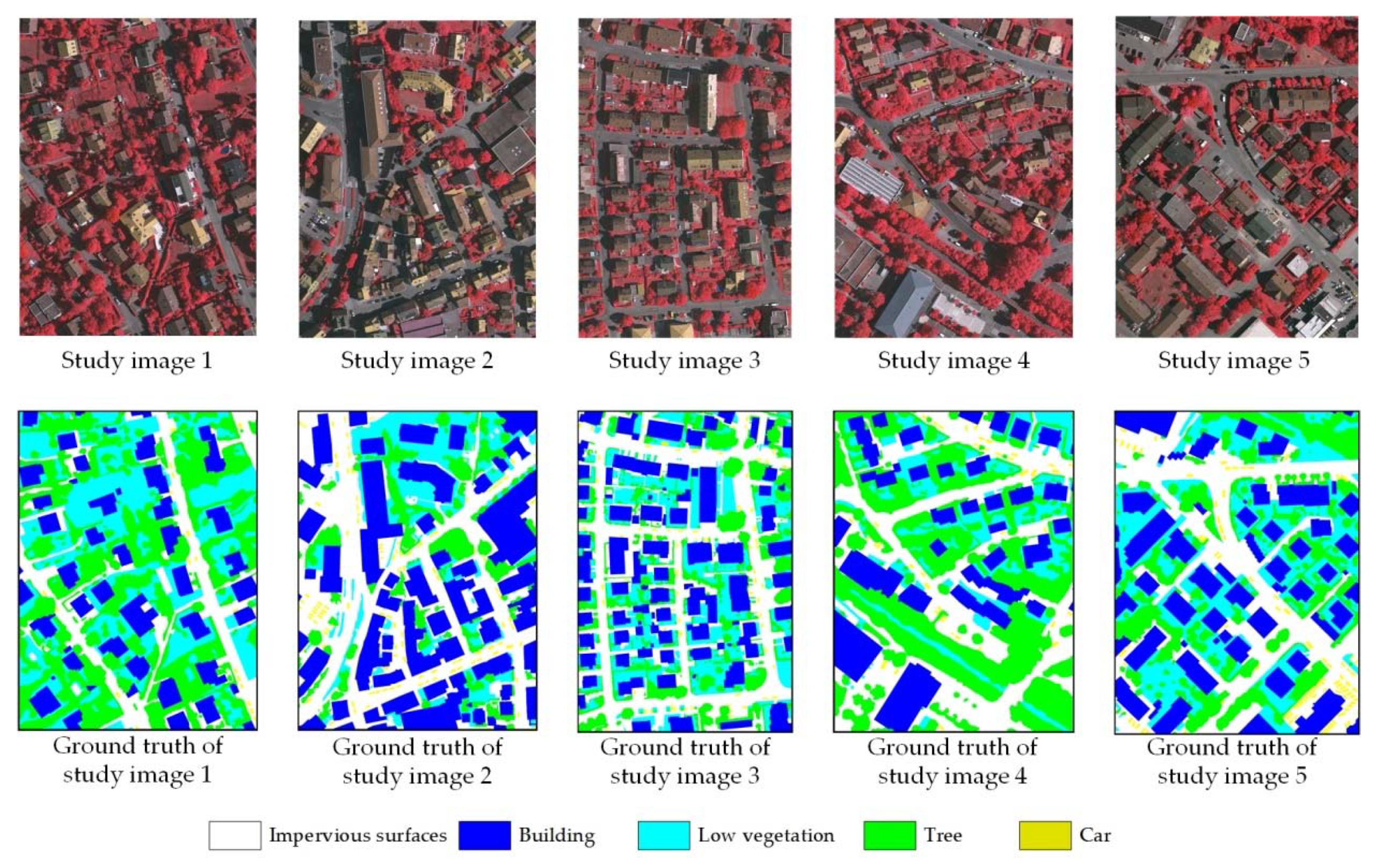
We introduced five commonly used DSSNN models as testing targets: FCN8s, FCN16s, FCN32s, SegNET, and U-Net. All these deep models are implemented using the Keras package, and all the models take a 224 × 224 image patch as input and output a corresponding semantic segmentation result. The five image files from Vaihingen were selected as the study images and are listed in Table 1.
All five images contain five categories: impervious surfaces (I), buildings (B), low vegetation (LV), trees (T), and cars (C). These images have three spatial bands (near-infrared (NIR), red (R), and green (G)). The study images and their corresponding ground truth images are shown in Figure 4.
We selected study images 1 and 3 as training data and used all the images as test data. Study images 1 and 3 and their ground truth images were cut into 224 × 224 image patches with 10-pixel intervals; all the patches were stacked into a training set, and all the deep semantic segmentation models were trained on this training set.
This study used two methods to compare correction ability:
(1) CRF: We compared our method with the traditional CRF method. For each classification result image, the CRF was executed 10 times, and each time, the corresponding correct-distance parameters were set to 10, 20, …, 100. Since all the study images have corresponding ground truth images, the CRF algorithm selects the result with the highest accuracy among the 10 executions.
(2) ELP: Using the proposed method, the threshold value parameter α was set to 0.05, and the CRF’s correct-distance parameters in the LocalizedCorrection algorithm were set to 10. The number of ELP iterations was set to 10. Since ELP emphasizes “end-to-end” ability, no ground truth is needed to analyze the true classification accuracy during the iteration process; therefore, ELP directly outputs the result of the last iteration as the corrected image.
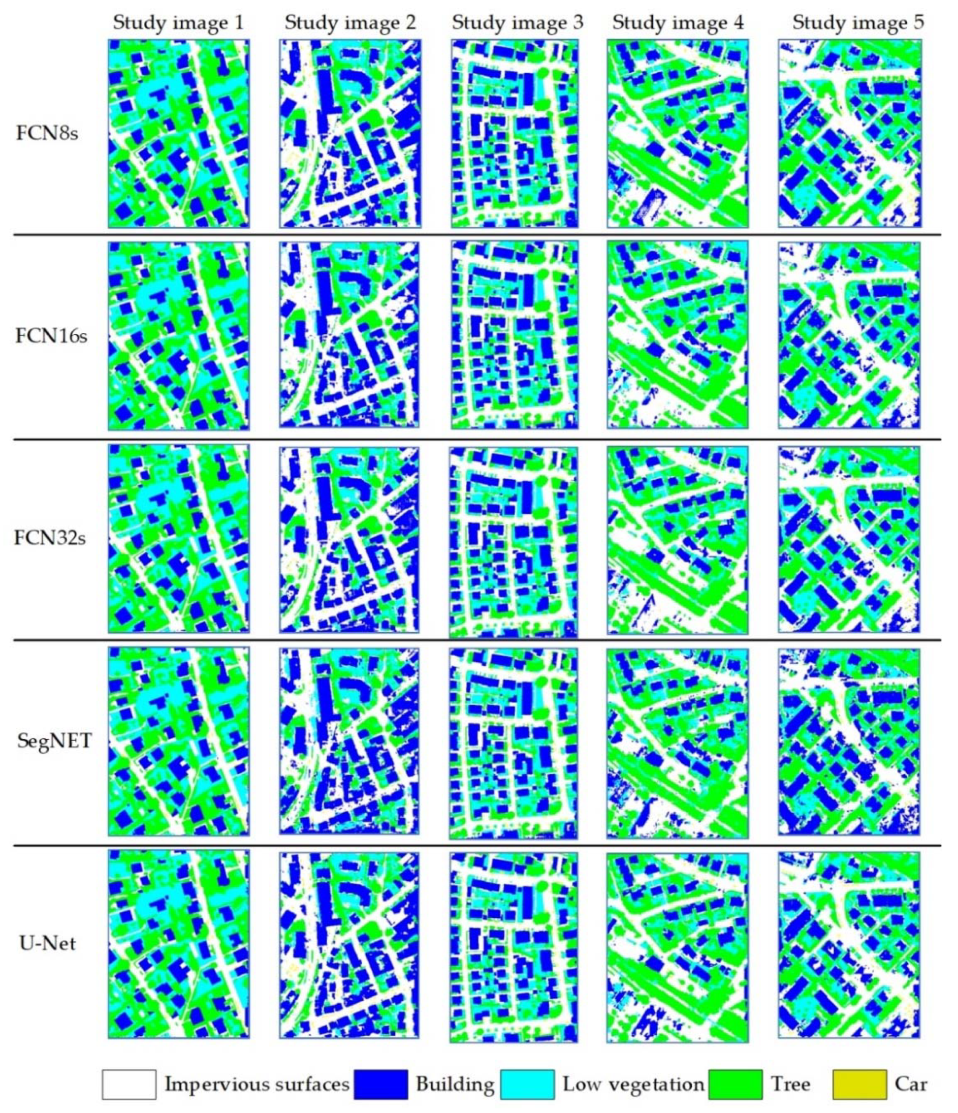
3.1.2. Classification Results of Semantic Segmentation Models
We used all five deep semantic segmentation models as end-to-end classifiers to process five study images. The classification results are illustrated in Figure 5.
As shown in Figure 5, because study images 1 and 3 are used as training data (the deep neural network is sufficiently large to “remember” these images), the classification results by the five models for study images 1 and 3 are close to “perfect”: almost all the ground objects and boundaries are correctly identified. However, because just two training images cannot exhaustively represent all the boundaries and object characteristics, these models cannot perfectly process study images 2, 4, and 5. As shown in Figure 5, there are obvious defects and boundary deformations, and many objects are misclassified in large areas. Based on the ground truth images, the classification accuracies of these result images are as follows:
As shown in Figure 5, because study images 1 and 3 are used as training data (the deep neural network is sufficiently large to “remember” these images), the classification results by the five models for study images 1 and 3 are close to “perfect”: almost all the ground objects and boundaries are correctly identified. However, because just two training images cannot exhaustively represent all the boundaries and object characteristics, these models cannot perfectly process study images 2, 4, and 5. As shown in Figure 5, there are obvious defects and boundary deformations, and many objects are misclassified in large areas. Based on the ground truth images, the classification accuracies of these result images are as follows:
Table 2 shows that because study images 1 and 3 are training images, all five models’ classification accuracies of these two images are above 95%, which is a satisfactory result. However, on study images 2, 4, and 5, due to the many errors on ground objects and boundaries, all five models’ classification accuracies degrade to approximately 80%. Therefore, it is necessary to introduce a correction mechanism to correct the boundary errors in these images.
3.1.3. Comparison of the Correction Characteristics of ELP and CRF
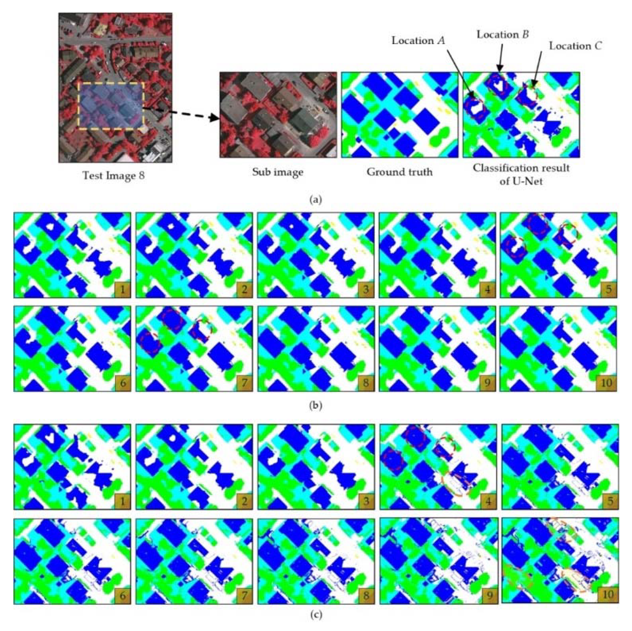
To compare the correction characteristics of the ELP and CRF, this section uses U-Net’s classification result for test image 5 and applies ELP and CRF to correct a subarea of the result image. The detailed results of the two algorithms with regard to iterations (ELP) and execution (CRF) are as shown in Figure 6.
As shown in Figure 6a, for the sub-image of test image 5, the classification results obtained by U-Net are far from perfect, and the boundaries of objects are blurred or chaotic. Especially at locations A, B, and C (marked by the red circles), the buildings are confused with impervious surfaces, and the buildings contain large holes or misclassified parts. On this sub-image, the classification accuracy of U-Net is only 79.02%.
Figure 6b shows the results of the 10 ELP iterations. As the method iterates, the object boundaries are gradually refined, and the errors at locations A and B are gradually corrected. By the 5th iteration, the hole at position A is completely filled, and by the 7th iteration, the errors at location B are also corrected. For location C, because our algorithm follows an end-to-end process, no samples exist in this process to determine which part of the corresponding area is incorrect; therefore, location C is not significantly modified during the iterations. Nevertheless, the initial classification error is not enlarged. As the iteration continues, the resulting images change little from the 7th to 10th iterations, and the algorithm’s result becomes stable.
Figure 6c shows the results of the CRF. From executions 1 to 3, it can be seen that the CRF can also perform boundary correction. After the 4th iteration, the errors in locations A and B are corrected. It can also be seen that at position C, part of the correctly classified building roof was modified into impervious surfaces, further exaggerating the errors. The reason for this outcome is that at location C, for the corresponding roof color, the correctly classified part is smaller than the misclassified part. In the global correction context, the CRF algorithm more easily replaces relatively small parts. At the same time, as the iteration progresses, errors gradually appear due to the CRF’s correction process (as marked in orange); some categories that were originally not dominant in an area (such as trees and cars) experience large decreases, and the classification accuracy continues to decrease with further iterations.
Based on the ground truth image, we evaluate the classification accuracy of the two methods after each iteration/execution as shown in Table 3:
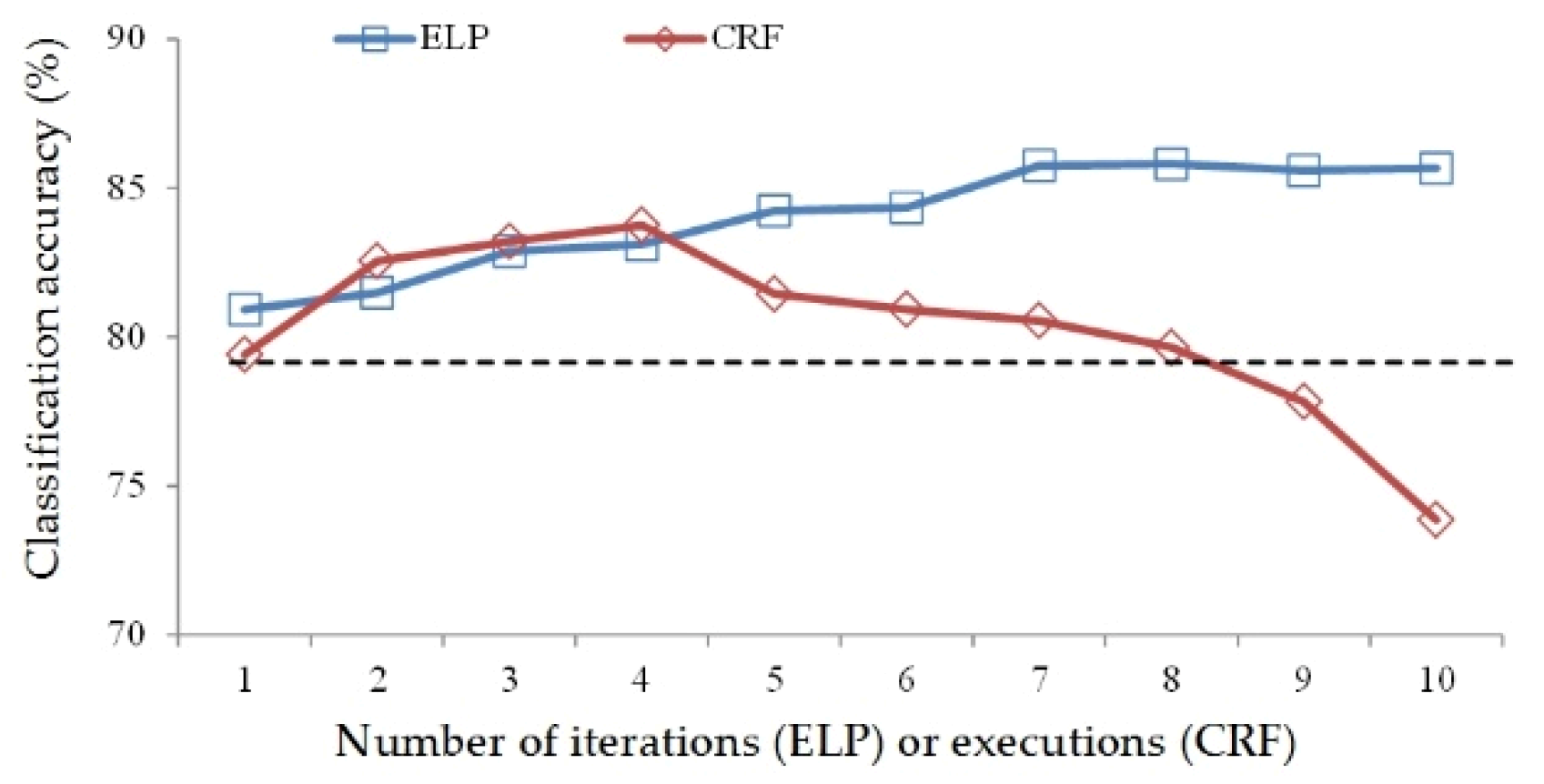
As seen from Table 3, compared to the original classification result, whose accuracy is 79.02%, the ELP’s classification accuracy increases to 80.93% after the first iteration—the lowest among its ten iterations, and it reaches 85.81% by the 8th iteration for a classification accuracy improvement of 6.79%. The CRF’s classification accuracy is 79.41% after the first executions, and it reaches its highest accuracy of 83.76% in the 4th execution; subsequently, the classification accuracy gradually declines during the remaining iterations, falling to 73.86% by the 10th execution. Overall, the CRF reduced the accuracy by 5.16% compared with the original classification image. A graphical comparison of the classification accuracy of the two methods is shown in Figure 7:
In Figure 7, the black dashed line indicates the original classification accuracy of 79.02%. The CRF’s accuracy improvement was slightly better than that of the ELP algorithm in the second, third, and fourth iterations; however, its classification accuracy decreases rapidly in the later iterations, and by the ninth iteration, the classification accuracy is lower than that of the original classification result image. In contrast, the classification accuracy of the ELP increases steadily, and after approaching its highest accuracy, in subsequent iterations the accuracy remains relatively stable. From the above results, the ELP not only achieves a better correction result but also avoids causing obvious classification accuracy reductions from performing too many iterations. In end-to-end application scenarios where no samples participate in the result evaluation, we cannot know when the highest correction result has been reached; thus, the ideal method of termination conditions are also unknown. Specifying a too-small distance parameter will cause under-correction, while a too-large parameter will cause over-correction. The relatively stable characteristics and greater accuracy of ELP clearly allow it to achieve better processing results than those of CRF.
3.1.4. Correction Results Comparison
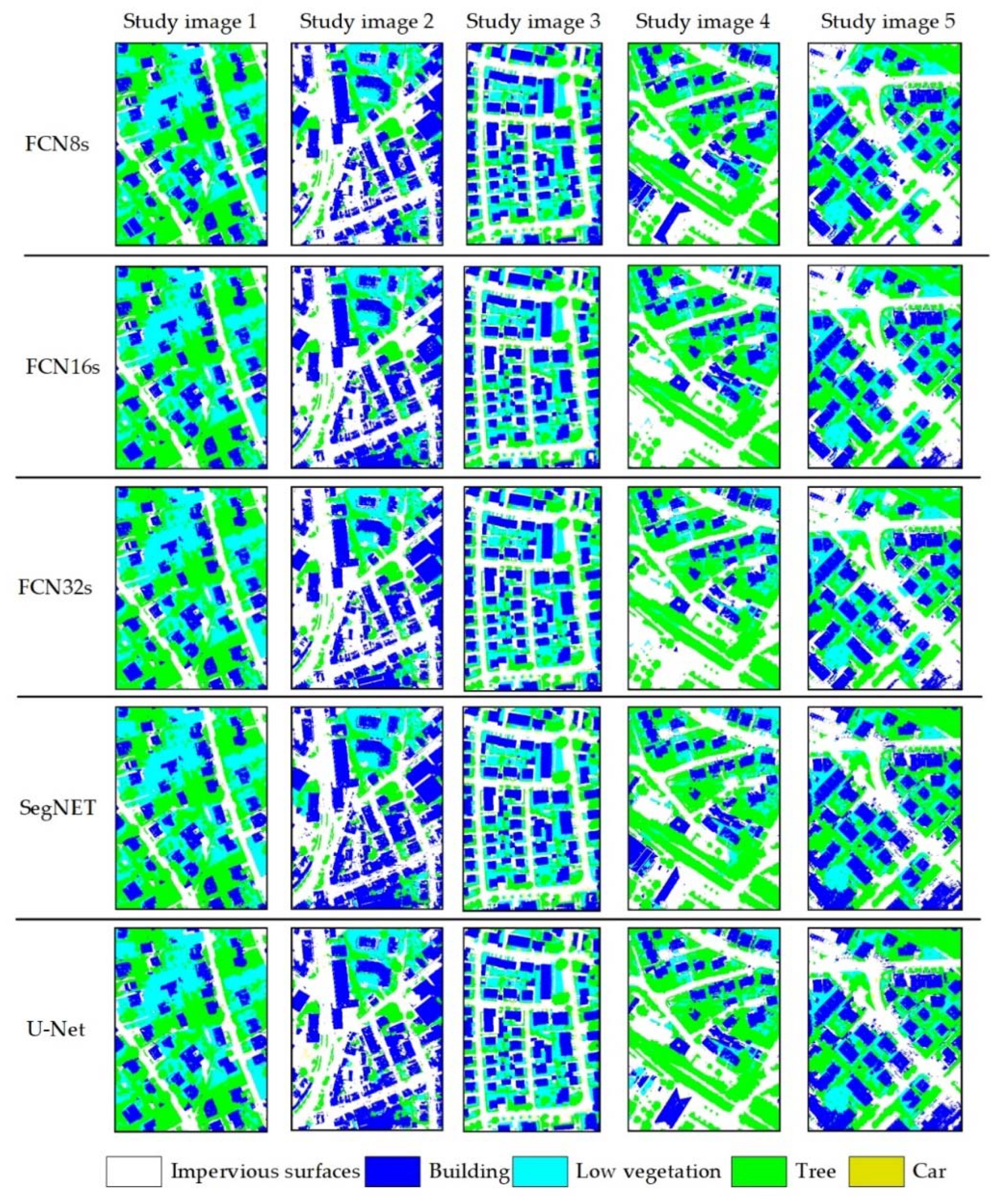
The correction results of the CRF method are shown in Figure 8.
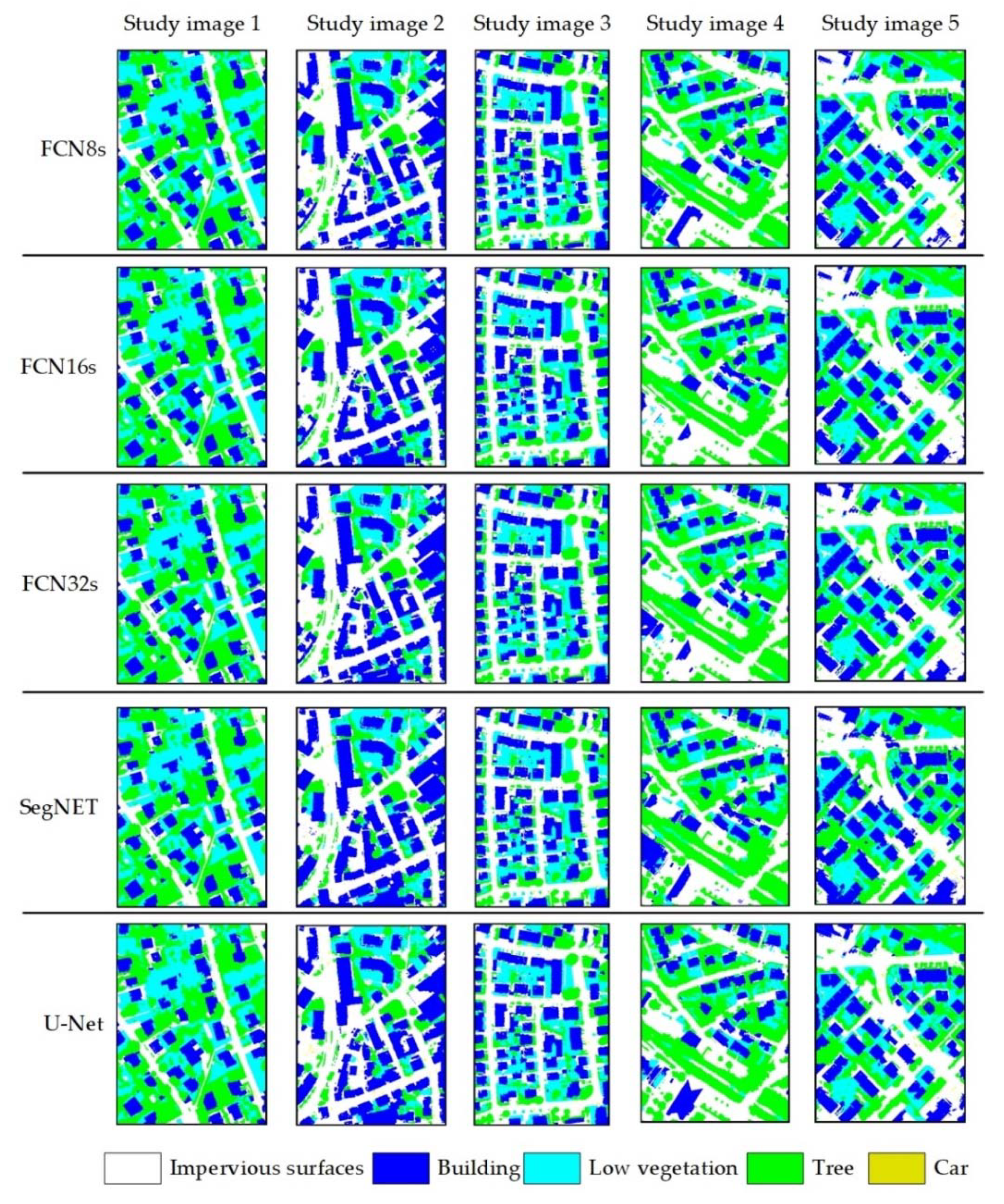
As shown in Figure 8, for images 1 and 3, because the classification accuracy is relatively high, less room exists for correction, and the resulting images change only slightly. For images 2, 4, and 5, although the large errors and holes are corrected, numerous incorrect borders are present, pixels appear at shadowed parts of the ground objects, and many small objects (e.g., cars or trees) are erased by larger objects (e.g., impervious surfaces or low vegetation). For ELP, the correction results are shown in Figure 9.
As Figure 9 shows, ELP also corrects the large errors and holes but does not produce overcorrection errors in the shadowed parts of the ground objects, and small objects are not erased. Therefore, in general, the correction results of ELP are better than those of CRF. Correction accuracy comparisons of the two algorithms are shown in Table 4.
As shown in Table 3, for study images 1 and 3, because the original classification accuracy is high, the correction results of CRF and ELP are similar to the original classification result, and the improvements are limited. On study images 2, 4, and 5, the ELP’s average improvements are 6.78%, 7.09%, and 5.83%, respectively, while the corresponding CRF improvements are only 2.84%, 2.88%, and 2.74%. Thus, ELP’s correction ability is significantly better than that of CRF.
3.2. Comparison of Multiple Post-Processing Methods on Potsdam Dataset
3.2.1. Test Images and Methods
This study introduces four images from the Potsdam dataset, which are listed in Table 5.
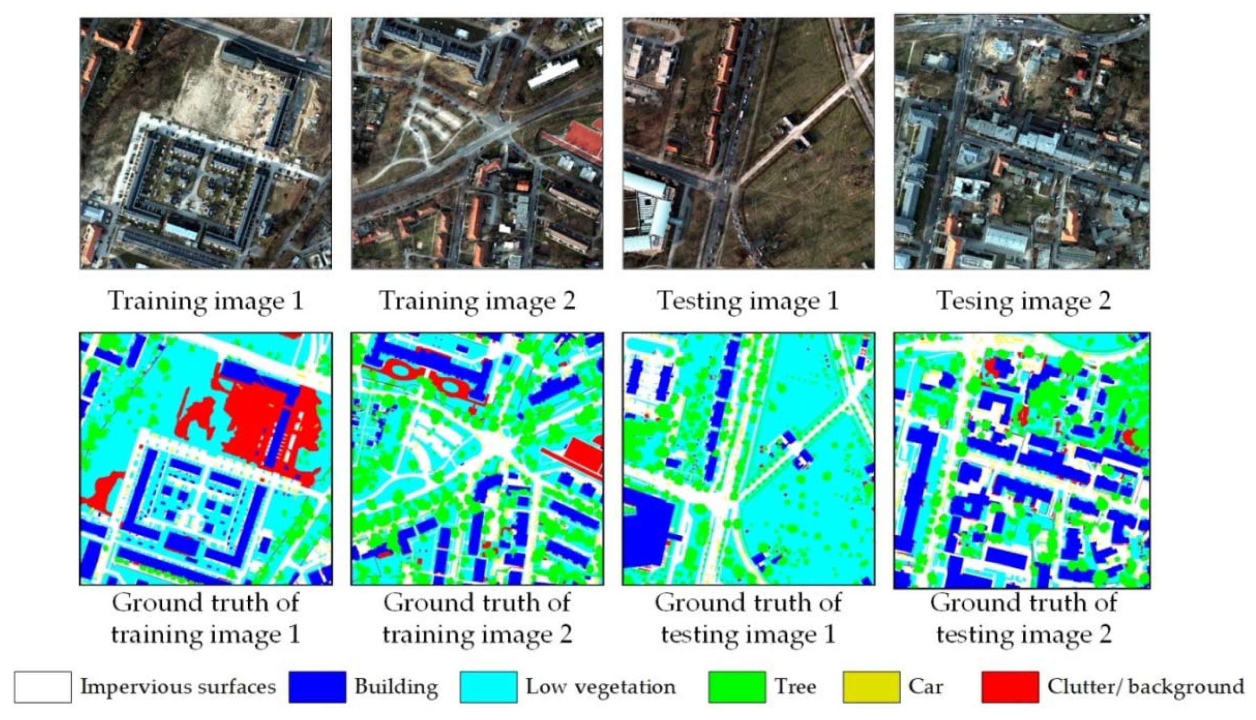
We selected two images as training data and the other two images as test data. Three bands (red (R), green (G), blue (B)) of images were selected. These images contain six categories: impervious surfaces (I), buildings (B), low vegetation (LV), trees (T), cars (C), and clutter/ background (C/B). The study images and their corresponding ground truth images are shown in Figure 10.
To further evaluate ELP’s ability, this paper compares four methods:
(1) U-Net + CRF: Use U-Net to classify an image and use CRF to perform post-processing.
(2) U-Net + MRF: Use U-Net to classify an image and use the Markov random field (MRF) to perform post-processing.
(3) DeepLab: Adopt DeepLab v1 model; in the DeepLab v1, the model has a built-in CRF as the last processing component, and this model can obtain a more accurate boundary than a model without the CRF component.
(4) U-Net + ELP: Use U-Net to classify an image and use ELP to perform post-processing.
3.2.2. Process Results of Four Methods
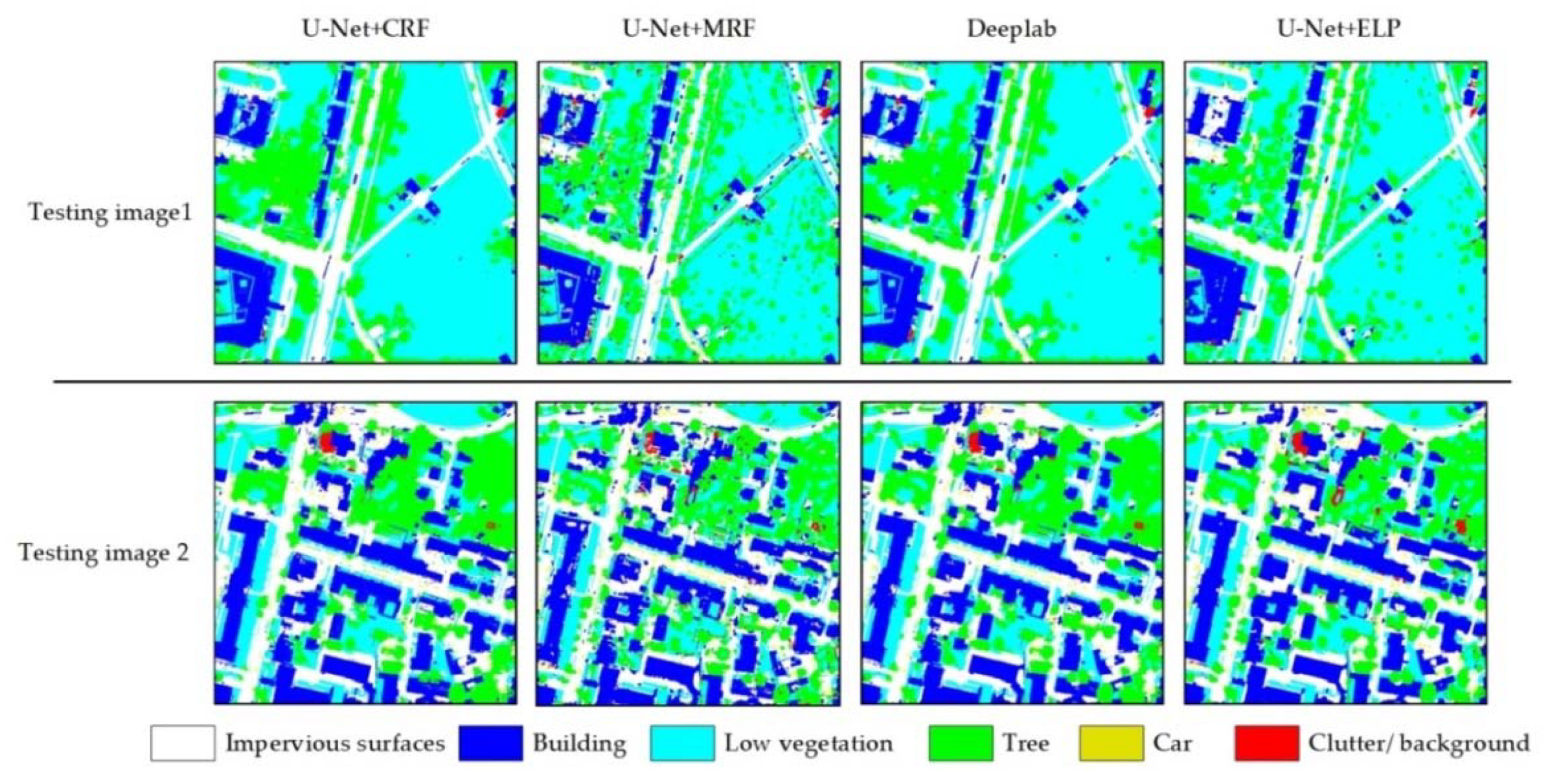
For the two testing images, the final process results of the four methods are illustrated in Figure 11.
As can be seen in Figure 11, because U-Net + CRF uses a global CRF processing strategy, there are many overcorrection areas, and some objects in the result image contain chaotic wrongly classified pixels. For the U-Net + MRF, the majority of noise pixels are removed, but the correction effects are not obvious. DeepLab’s CRF is performed on image patch, not the whole image, so the overcorrection phenomenon is less than that of U-Net + CRF to some extent. U-Net + ELP obtained the best classification among all of the methods. The classification accuracies of the four methods are presented in Table 6.
As shown in Table 6, U-Net + MRF achieves the lowest classification accuracy, U-Net + CRF and DeepLab are higher than U-Net + MRF, and U-Net + ELP achieves the best classification accuracy.
3.2.3. Analysis of computational complexity
To analyze the computational complexity of the methods, we use four methods to process the testing image 1 and run the process five times. The experiments are performed on a computer (i9 9900k/64 GB/RTX 2080ti 11G), and the average process times are listed in Table 7.
As shown in Table 7, because the U-Net model can make full use of the graphics processing unit (GPU), and the processing speed of CRF and MRF on the whole image is also fast, U-Net + CRF and U-Net + MRF obtain results in a short time. DeepLab performs CRF after each image patch classification, so it does not need the post-processing stage, but the patch-based CRF process needs additional data access time and duplicate pixels at the patches’ border, so its process time is similar to that of U-Net + CRF and U-Net + MRF. Since U-Net + ELP adopts the same deep model, its process time of the first three steps is similar to that of U-Net + CRF and U-Net + MRF, but at the post-processing stage, it needs a much longer time than the other methods.
For the ELP algorithm, the HList is updated at each iteration, and the suspicious areas marked by HList will change constantly. Each suspicious area needs to be processed by the CRF method, so the processing complexity of the ELP will vary along with the complexity of the image content. Although each suspicious area is small, ELP’s greater amount of iterations, localization process, and result image update mechanism will introduce an additional computational burden, so ELP needs more process time than traditional methods.
3.2.4. Analysis of Different Threshold Parameter Values of ELP
The threshold value α of ELP will determine the choice of suspicious areas. To test the influence of this parameter, we chose UNet + ELP to process testing image 1, and set α in the range 0, 0.01, 0.02, …, 0.09, which can vary from 0 to 0.09 with an interval of 0.01. The classification accuracy is shown in Table 8.
As can be seen from Table 8, when α is less than 0.6, the classification accuracy does not change significantly; when α is larger than 0.7, the classification accuracy is decreased. The main reason for this phenomenon is that when α is small, ELP will be more sensitive to the discovery of suspicious areas; however, too many suspicious areas merely increase the computational burden without contributing to obvious changes in accuracy. In contrast, when α is larger, ELP will have a diminished capability to discover suspicious areas, and many suspicious areas that need correction will be omitted, which will cause a decrease in accuracy. At the same time, we can see from Table 8 that in a large range (0.0 to 0.6), the accuracy of ELP does not change greatly, which reveals that ELP has good stability with the threshold value α.
3.2.5. Analysis of Different Segmentation Number of ELP
The ELP method adopts the SLIC algorithm as the segmentation method, and an important parameter of the SLIC algorithm is Nsegment which decides the number of segments after the algorithm performed. When the Nsegment is assigned an overly small value, under-segmentation may appear; conversely, when Nsegment is assigned an overly large value, over-segmentation may appear. To test the influence of this parameter on the ELP, we set Nsegment = 1000, 2000, …, 10,000 and allowed Nsegment to vary from 1000 to 10,000 with an interval of 1000. The classification accuracy of testing image 1 by U-Net + ELP is shown in Table 9.
It can be seen from Table 9 that when Nsegment = 1000 to 3000, because the image is large (6000 × 6000) and the segment number is relatively small, the image is under-segmented, and each segmentation may contain pixels with a different color or brightness. This situation makes it difficult for ELP to focus on suspicious areas, and the classification accuracy is low. When Nsegment = 9000 to 10,000, the image is obviously over-segmented, and the segmentations are too small. This situation leads ELP to have a small update size in its LocalizedCorrection algorithm and leads to ELP’s poor performance. For Nsegment = 4000 to 8000, the classification accuracy of ELP does not vary greatly, which indicates that ELP does not have restrictive requirements for the segment parameter; as long as the segment method can correctly separate the regions with similar colors/brightness and the segment size is not too small, ELP can achieve satisfactory results.
4. Conclusions
Deep semantic segmentation neural networks are powerful end-to-end remote sensing image classification tools that have achieved successes in many applications. However, it is difficult to construct a training set that thoroughly exhausts all the pixel segmentation possibilities for a specific ground area; in addition, spatial information loss occurs during the network training and inference stages. Consequently, the classification results of DSSNNs are usually not perfect, which introduces a need to correct the results.
Our experiments demonstrate that when faced with complicated remote sensing images, the CRF algorithm often has difficulty achieving a substantially improved correction effect; without restricting the mechanism by using additional samples, the CRF may overcorrect, leading to a decrease in the classification accuracy. Our approach improves on the traditional CRF global processing effects by offering two advantages:
(1) End-to-end: ELP identifies which locations of the result image are highly suspected of containing errors without requiring samples; this characteristic allows ELP to be used in an end-to-end classification process.
(2) Localization: Based on the suspect areas, ELP limits the CRF analysis and update area within a small range and controls the iteration termination condition; these characteristics avoid the overcorrections caused by the global processing of the CRF.
The experimental results also show that the ELP achieves a better correction result, is more stable, and does not require training samples to restrict the iterations. The above advantages ensure that ELP is better able to adapt to correct the classification results of remote sensing images and provides it with a higher degree of automation.
The typical limitation of ELP is that, in comparison with the traditional CRF, the additional iterations, the localization process, and the update mechanism of the result image will introduce an additional computational burden. Consequently, ELP is much slower than the traditional CRF method. Fortunately, the localization process also ensures that different parts of areas do not affect each other, which makes ELP easier to parallelize. In further research, we will adjust the processing structure of ELP, facilitating a GPU implementation that enables ELP to execute faster. For semantic segmentation neural networks, differences in the training set size can cause various degrees of errors in the resulting image, which has an apparent influence on the post-processing task. In future research, to construct a more adaptive post-processing method, we will study the relationship between training/testing dataset size and the post-processing methods used and consider the problems faced by post-processing methods in more complex application scenarios.
Author Contributions
Conceptualization, X.P. and J.X.; data curation, J.Z.; methodology, X.P.; supervision, J.X.; visualization, J.Z.; writing—original draft, X.P. All authors have read and agree to the published version of the manuscript.
Funding
This research was jointly supported by the National Natural Science Foundation of China (41871236; 41971193) and the Natural Science Foundation of Jilin Province (20180101020JC).
Conflicts of Interest
The authors declare no conflict of interest.
References
- Pan, X.; Zhao, J.; Xu, J. An object-based and heterogeneous segment filter convolutional neural network for high-resolution remote sensing image classification. Int. J. Remote Sens. 2019, 40, 5892–5916. [Google Scholar] [CrossRef]
- Tong, X.-Y.; Xia, G.-S.; Lu, Q.; Shen, H.; Li, S.; You, S.; Zhang, L. Land-cover classification with high-resolution remote sensing images using transferable deep models. Remote Sens. Environ. 2020, 237, 111322. [Google Scholar] [CrossRef] [Green Version]
- Pan, X.; Zhao, J. A central-point-enhanced convolutional neural network for high-resolution remote-sensing image classification. Int. J. Remote Sens. 2017, 38, 6554–6581. [Google Scholar] [CrossRef]
- Chen, Y.Y.; Ming, D.P.; Lv, X.W. Superpixel based land cover classification of VHR satellite image combining multi-scale CNN and scale parameter estimation. Earth Sci. Inform. 2019, 12, 341–363. [Google Scholar] [CrossRef]
- Long, J.; Shelhamer, E.; Darrell, T. Fully Convolutional Networks for Semantic Segmentation. In Proceedings of the rfgvb 2015 Ieee Conference on Computer Vision and Pattern Recognition (Cvpr), Boston, MA, USA, 7–12 June 2015; pp. 3431–3440. [Google Scholar]
- Zhu, X.X.; Tuia, D.; Mou, L.; Xia, G.S.; Zhang, L.; Xu, F.; Fraundorfer, F. Deep learning in remote sensing: A Comprehensive Review and List of Resources. IEEE Geosci. Remote Sens. Mag. 2017, 5, 8–36. [Google Scholar] [CrossRef] [Green Version]
- Long, J.; Shelhamer, E.; Darrell, T. Fully convolutional networks for semantic segmentation. In Proceedings of the IEEE Conference on Computer Vision and Pattern Recognition, Boston, MA, USA, 7–12 June 2015; pp. 3431–3440. [Google Scholar] [CrossRef] [Green Version]
- Badrinarayanan, V.; Kendall, A.; Cipolla, R. SegNet: A Deep Convolutional Encoder-Decoder Architecture for Image Segmentation. IEEE Trans. Pattern Anal. Mach. Intell. 2017, 39, 2481–2495. [Google Scholar] [CrossRef]
- Ronneberger, O.; Fischer, P.; Brox, T. U-Net: Convolutional Networks for Biomedical Image Segmentation. In Medical Image Computing and Computer-Assisted Intervention, Pt Iii; Springer: Munich, Germany, 2015; Volume 9351, pp. 234–241. [Google Scholar] [CrossRef] [Green Version]
- Kemker, R.; Salvaggio, C.; Kanan, C. Algorithms for semantic segmentation of multispectral remote sensing imagery using deep learning. Isprs J. Photogramm. 2018, 145, 60–77. [Google Scholar] [CrossRef] [Green Version]
- Vakalopoulou, M.; Karantzalos, K.; Komodakis, N.; Paragios, N. Building Detection in Very High Resolution Multispectral Data with Deep Learning Features. In Proceedings of the 2015 IEEE International Geoscience and Remote Sensing Symposium (IGARSS), Milan, Italy, 26–31 July 2015; pp. 1873–1876. [Google Scholar] [CrossRef] [Green Version]
- Yi, Y.N.; Zhang, Z.J.; Zhang, W.C.; Zhang, C.R.; Li, W.D.; Zhao, T. Semantic Segmentation of Urban Buildings from VHR Remote Sensing Imagery Using a Deep Convolutional Neural Network. Remote Sens.-Basel 2019, 11, 1774. [Google Scholar] [CrossRef] [Green Version]
- Zhou, L.C.; Zhang, C.; Wu, M. D-LinkNet: LinkNet with Pretrained Encoder and Dilated Convolution for High Resolution Satellite Imagery Road Extraction. In Proceedings of the 2018 IEEE/CVF Conference on Computer Vision and Pattern Recognition Workshops (CVPRW), Salt Lake City, UT, USA, 18–22 June 2018; pp. 192–196. [Google Scholar] [CrossRef]
- Tao, C.; Qi, J.; Li, Y.S.; Wang, H.; Li, H.F. Spatial information inference net: Road extraction using road-specific contextual information. Isprs J. Photogramm. 2019, 158, 155–166. [Google Scholar] [CrossRef]
- Zhang, Z.X.; Liu, Q.J.; Wang, Y.H. Road Extraction by Deep Residual U-Net. IEEE Geosci. Remote Sens. 2018, 15, 749–753. [Google Scholar] [CrossRef] [Green Version]
- Volpi, M.; Tuia, D. Dense Semantic Labeling of Subdecimeter Resolution Images with Convolutional Neural Networks. IEEE Trans. Geosci. Remote 2017, 55, 881–893. [Google Scholar] [CrossRef] [Green Version]
- Chen, G.Z.; Zhang, X.D.; Wang, Q.; Dai, F.; Gong, Y.F.; Zhu, K. Symmetrical Dense-Shortcut Deep Fully Convolutional Networks for Semantic Segmentation of Very-High-Resolution Remote Sensing Images. IEEE J.-Stars 2018, 11, 1633–1644. [Google Scholar] [CrossRef]
- Mohammadimanesh, F.; Salehi, B.; Mandianpari, M.; Gill, E.; Molinier, M. A new fully convolutional neural network for semantic segmentation of polarimetric SAR imagery in complex land cover ecosystem. Isprs J. Photogramm. 2019, 151, 223–236. [Google Scholar] [CrossRef]
- Mboga, N.; Georganos, S.; Grippa, T.; Lennert, M.; Vanhuysse, S.; Wolff, E. Fully Convolutional Networks and Geographic Object-Based Image Analysis for the Classification of VHR Imagery. Remote Sens. 2019, 11, 597. [Google Scholar] [CrossRef] [Green Version]
- Mi, L.; Chen, Z. Superpixel-enhanced deep neural forest for remote sensing image semantic segmentation. Isprs J. Photogramm. 2020, 159, 140–152. [Google Scholar] [CrossRef]
- Fu, G.; Liu, C.J.; Zhou, R.; Sun, T.; Zhang, Q.J. Classification for High Resolution Remote Sensing Imagery Using a Fully Convolutional Network. Remote Sens. 2017, 9, 498. [Google Scholar] [CrossRef] [Green Version]
- Marmanis, D.; Schindler, K.; Wegner, J.D.; Galliani, S.; Datcu, M.; Stilla, U. Classification with an edge: Improving semantic image segmentation with boundary detection. Isprs J. Photogramm. 2018, 135, 158–172. [Google Scholar] [CrossRef] [Green Version]
- Lafferty, J.D.; McCallum, A.; Pereira, F.C.N. Conditional random fields: Probabilistic models for segmenting and labeling sequence data. In Proceedings of the Eighteenth International Conference on Machine Learning (ICML 2001), Williamstown, MA, USA, 28 June–1 July 2001; pp. 282–289. [Google Scholar]
- Alam, F.I.; Zhou, J.; Liew, A.W.C.; Jia, X.P. Crf learning with cnn features for hyperspectral image segmentation. In Proceedings of the 2016 Ieee International Geoscience and Remote Sensing Symposium (Igarss), Beijing, China, 10–15 July 2016; pp. 6890–6893. [Google Scholar]
- Zhang, B.; Wang, C.P.; Shen, Y.L.; Liu, Y.Y. Fully Connected Conditional Random Fields for High-Resolution Remote Sensing Land Use/Land Cover Classification with Convolutional Neural Networks. Remote Sens. 2018, 10, 1889. [Google Scholar] [CrossRef] [Green Version]
- Zheng, S.; Jayasumana, S.; Romera-Paredes, B.; Vineet, V.; Su, Z.Z.; Du, D.L.; Huang, C.; Torr, P.H.S. Conditional Random Fields as Recurrent Neural Networks. In Proceedings of the 2015 IEEE International Conference on Computer Vision (ICCV), Santiago, Chile, 7–13 December 2015; pp. 1529–1537. [Google Scholar] [CrossRef] [Green Version]
- Chen, Y.S.; Zhao, X.; Jia, X.P. Spectral-Spatial Classification of Hyperspectral Data Based on Deep Belief Network. IEEE J.-Stars 2015, 8, 2381–2392. [Google Scholar] [CrossRef]
- Marmanis, D.; Wegner, J.D.; Galliani, S.; Schindler, K.; Datcu, M.; Stilla, U. Semantic segmentation of aerial images with an ensemble of cnss. In Proceedings of the ISPRS Annals of the Photogrammetry, Remote Sensing and Spatial Information Sciences, Prag, Tschechien, 12–19 July 2016; Volume 3, pp. 473–480. [Google Scholar]
- Maggiori, E.; Tarabalka, Y.; Charpiat, G.; Alliez, P. Fully Convolutional Neural Networks for Remote Sensing Image Classification. In Proceedings of the 2016 Ieee International Geoscience and Remote Sensing Symposium (Igarss), Beijing, China, 10–15 July 2016; pp. 5071–5074. [Google Scholar] [CrossRef] [Green Version]
- He, C.; Fang, P.Z.; Zhang, Z.; Xiong, D.H.; Liao, M.S. An End-to-End Conditional Random Fields and Skip-Connected Generative Adversarial Segmentation Network for Remote Sensing Images. Remote Sens. 2019, 11, 1604. [Google Scholar] [CrossRef] [Green Version]
- Pan, X.; Zhao, J. High-Resolution Remote Sensing Image Classification Method Based on Convolutional Neural Network and Restricted Conditional Random Field. Remote Sens. 2018, 10, 920. [Google Scholar] [CrossRef] [Green Version]
- Ma, F.; Gao, F.; Sun, J.P.; Zhou, H.Y.; Hussain, A. Weakly Supervised Segmentation of SAR Imagery Using Superpixel and Hierarchically Adversarial CRF. Remote Sens. 2019, 11, 512. [Google Scholar] [CrossRef] [Green Version]
- Wei, L.F.; Yu, M.; Zhong, Y.F.; Zhao, J.; Liang, Y.J.; Hu, X. Spatial-Spectral Fusion Based on Conditional Random Fields for the Fine Classification of Crops in UAV-Borne Hyperspectral Remote Sensing Imagery. Remote Sens. 2019, 11, 780. [Google Scholar] [CrossRef] [Green Version]
- Parente, L.; Taquary, E.; Silva, A.P.; Souza, C.; Ferreira, L. Next Generation Mapping: Combining Deep Learning, Cloud Computing, and Big Remote Sensing Data. Remote Sens. 2019, 11, 2881. [Google Scholar] [CrossRef] [Green Version]
- Kampffmeyer, M.; Salberg, A.B.; Jenssen, R. Semantic Segmentation of Small Objects and Modeling of Uncertainty in Urban Remote Sensing Images Using Deep Convolutional Neural Networks. In Proceedings of the 29th Ieee Conference on Computer Vision and Pattern Recognition Workshops, (Cvprw 2016), Las Vegas, NV, USA, 26 June–1 July 2016; pp. 680–688. [Google Scholar] [CrossRef]
- Achanta, R.; Shaji, A.; Smith, K.; Lucchi, A.; Fua, P.; Susstrunk, S. SLIC Superpixels Compared to State-of-the-Art Superpixel Methods. IEEE Trans. Pattern Anal. 2012, 34, 2274–2281. [Google Scholar] [CrossRef] [PubMed] [Green Version]
Figure 1.
End-to-end classification strategy.

Figure 2.
End-to-end result image evaluation and localized post-processing.

Figure 3.
Overall processes of end-to-end and localized post-processing method (ELP).

Figure 4.
The study images and their corresponding ground truth from the Vaihingen dataset.

Figure 5.
Classification results of five deep semantic segmentation models.

Figure 6.
Detailed comparison of the results of the ELP and conditional random field (CRF) algorithms. (a) Ground truth and U-Net’s classification results of a subarea of test image 5; (b) results of ten iterations of ELP; (c) results of ten executions of CRF.
Figure 6.
Detailed comparison of the results of the ELP and conditional random field (CRF) algorithms. (a) Ground truth and U-Net’s classification results of a subarea of test image 5; (b) results of ten iterations of ELP; (c) results of ten executions of CRF.

Figure 7.
Graphical comparison of the classification accuracy of the two methods.

Figure 8.
CRF correction results.

Figure 9.
ELP correction results.

Figure 10.
The study images and their corresponding ground truth from the Potsdam dataset.

Figure 11.
Results of the four methods.


Table 1.
Five study images from the Vaihingen dataset.
| Image ID | Filename | Size | Role |
|---|---|---|---|
| 1 | top_mosaic_09cm_area23.tif | 1903 × 2546 | Training/Testing image |
| 2 | top_mosaic_09cm_area1.tif | 1919 × 2569 | Testing image |
| 3 | top_mosaic_09cm_area3.tif | 2006 × 3007 | Training/Testing image |
| 4 | top_mosaic_09cm_area21.tif | 1903 × 2546 | Testing image |
| 5 | top_mosaic_09cm_area30.tif | 1934 × 2563 | Testing image |
Table 2.
Classification accuracy for the study images.
| Model | Classification Accuracy of Study Images (%) | ||||
|---|---|---|---|---|---|
| 1 | 2 | 3 | 4 | 5 | |
| FCN8s | 97.46 | 81.92 | 96.16 | 79.52 | 80.37 |
| FCN16s | 96.90 | 79.61 | 95.04 | 76.98 | 80.12 |
| FCN32s | 97.22 | 82.27 | 95.01 | 78.59 | 81.63 |
| SegNET | 97.83 | 78.95 | 95.39 | 76.50 | 77.11 |
| U-Net | 97.91 | 82.02 | 97.38 | 79.43 | 80.07 |
Table 3.
Comparison of two algorithms by iteration/execution.
| Methods | Classification Accuracy at each Iteration/Execution (%) | |||||||||
|---|---|---|---|---|---|---|---|---|---|---|
| 1 | 2 | 3 | 4 | 5 | 6 | 7 | 8 | 9 | 10 | |
| ELP | 80.93 | 81.49 | 82.88 | 83.11 | 84.24 | 84.34 | 85.76 | 85.81 | 85.59 | 85.67 |
| CRF | 79.41 | 82.55 | 83.21 | 83.76 | 81.45 | 80.93 | 80.55 | 79.65 | 77.83 | 73.86 |
Table 4.
Correction accuracy comparisons of CRF and ELP.
| Model | Classification Accuracy of Study Images (%) | |||||||||
|---|---|---|---|---|---|---|---|---|---|---|
| 1 | 2 | 3 | 4 | 5 | ||||||
| CRF | ELP | CRF | ELP | CRF | ELP | CRF | ELP | CRF | ELP | |
| FCN8s | 97.91 | 97.88 | 84.72 | 88.32 | 97.31 | 97.02 | 81.24 | 85.47 | 82.81 | 85.87 |
| FCN16s | 97.41 | 97.37 | 83.33 | 87.61 | 96.94 | 97.11 | 80.57 | 84.67 | 84.02 | 85.82 |
| FCN32s | 97.67 | 97.62 | 84.90 | 87.32 | 96.71 | 96.31 | 82.02 | 84.89 | 83.02 | 85.70 |
| SegNET | 97.89 | 97.94 | 80.98 | 86.51 | 96.44 | 97.03 | 80.07 | 84.51 | 80.05 | 85.01 |
| U-Net | 97.95 | 97.98 | 85.07 | 88.91 | 97.42 | 97.47 | 81.53 | 86.93 | 83.12 | 86.07 |
| Average Improvement | 0.30 | 0.29 | 2.84 | 6.78 | 1.16 | 1.19 | 2.88 | 7.09 | 2.74 | 5.83 |
Table 5.
Four study images from the Potsdam dataset.
| Image Name | Filename | Size |
|---|---|---|
| Training image 1 | top_potsdam_2_10_RGBIR | 6000 × 6000 |
| Training image 2 | top_potsdam_3_10_RGBIR | 6000 × 6000 |
| Testing image 1 | top_potsdam_2_12_RGBIR | 6000 × 6000 |
| Testing image 2 | top_potsdam_3_12_RGBIR | 6000 × 6000 |
Table 6.
Classification accuracies of the four methods.
| Image File | Classification Accuracy of the Four Methods (%) | |||
|---|---|---|---|---|
| U-Net + CRF | U-Net + MRF | DeepLab | U-Net + ELP | |
| Testing image 1 | 81.67 | 78.45 | 82.85 | 85.31 |
| Testing image 2 | 80.49 | 76.33 | 83.57 | 86.58 |
Table 7.
Process time of four methods.
| Methods | Process Time of Each Step (Seconds) | Overall Time (Seconds) | |||
|---|---|---|---|---|---|
| Image Separate | Patches Classification | Patches Combination | Post-Processing | ||
| U-Net + CRF | 7.52 | 45.84 | 8.32 | 216.34 | 278.02 |
| U-Net + MRF | 7.43 | 45.67 | 8.51 | 170.97 | 232.58 |
| DeepLab | 7.61 | 232.98 | 8.45 | \ | 249.04 |
| U-Net + ELP | 7.57 | 46.02 | 8.77 | 506.45 | 568.81 |
Table 8.
Classification accuracy comparison of different threshold values α.
| Method | Classification Accuracy at Different Threshold Parameter Value (%) | |||||||||
|---|---|---|---|---|---|---|---|---|---|---|
| 0.00 | 0.01 | 0.02 | 0.03 | 0.04. | 0.05 | 0.06 | 0.07 | 0.08 | 0.09 | |
| U-Net + ELP | 84.97 | 85.40 | 85.01 | 85.07 | 85.37 | 85.31 | 84.87 | 83.13 | 81.29 | 80.46 |
Table 9.
Classification accuracy comparison of different segment number.
| Method | Classification Accuracy at Different Segment Number (%) | |||||||||
|---|---|---|---|---|---|---|---|---|---|---|
| 1000 | 2000 | 3000 | 4000 | 5000 | 6000 | 7000 | 8000 | 9000 | 10,000 | |
| U-Net + ELP | 81.75 | 82.02 | 83.21 | 85.22 | 85.31 | 85.52 | 85.67 | 85.23 | 82.22 | 80.32 |
© 2020 by the authors. Licensee MDPI, Basel, Switzerland. This article is an open access article distributed under the terms and conditions of the Creative Commons Attribution (CC BY) license (http://creativecommons.org/licenses/by/4.0/).
Share and Cite
MDPI and ACS Style
Pan, X.; Zhao, J.; Xu, J. An End-to-End and Localized Post-Processing Method for Correcting High-Resolution Remote Sensing Classification Result Images. Remote Sens. 2020, 12, 852. https://0-doi-org.brum.beds.ac.uk/10.3390/rs12050852
AMA Style
Pan X, Zhao J, Xu J. An End-to-End and Localized Post-Processing Method for Correcting High-Resolution Remote Sensing Classification Result Images. Remote Sensing. 2020; 12(5):852. https://0-doi-org.brum.beds.ac.uk/10.3390/rs12050852
Chicago/Turabian StylePan, Xin, Jian Zhao, and Jun Xu. 2020. "An End-to-End and Localized Post-Processing Method for Correcting High-Resolution Remote Sensing Classification Result Images" Remote Sensing 12, no. 5: 852. https://0-doi-org.brum.beds.ac.uk/10.3390/rs12050852
Note that from the first issue of 2016, this journal uses article numbers instead of page numbers. See further details here.