Multi-scale Adaptive Feature Fusion Network for Semantic Segmentation in Remote Sensing Images

Abstract

Semantic segmentation of high-resolution remote sensing images is highly challenging due to the presence of a complicated background, irregular target shapes, and similarities in the appearance of multiple target categories. Most of the existing segmentation methods that rely only on simple fusion of the extracted multi-scale features often fail to provide satisfactory results when there is a large difference in the target sizes. Handling this problem through multi-scale context extraction and efficient fusion of multi-scale features, in this paper we present an end-to-end multi-scale adaptive feature fusion network (MANet) for semantic segmentation in remote sensing images. It is a coding and decoding structure that includes a multi-scale context extraction module (MCM) and an adaptive fusion module (AFM). The MCM employs two layers of atrous convolutions with different dilatation rates and global average pooling to extract context information at multiple scales in parallel. MANet embeds the channel attention mechanism to fuse semantic features. The high- and low-level semantic information are concatenated to generate global features via global average pooling. These global features are used as channel weights to acquire adaptive weight information of each channel by the fully connected layer. To accomplish an efficient fusion, these tuned weights are applied to the fused features. Performance of the proposed method has been evaluated by comparing it with six other state-of-the-art networks: fully convolutional networks (FCN), U-net, UZ1, Light-weight RefineNet, DeepLabv3+, and APPD. Experiments performed using the publicly available Potsdam and Vaihingen datasets show that the proposed MANet significantly outperforms the other existing networks, with overall accuracy reaching 89.4% and 88.2%, respectively and with average of F1 reaching 90.4% and 86.7% respectively.

1. Introduction

With the advancement of global observation technology and the development of increasingly higher-resolution sensors, it is now possible to acquire very high-resolution remote sensing images. Such images can capture detailed ground information, and facilitate the accurate analysis of scenes, and also objects within scenes. With the availability of high-resolution remote sensing images, the demand for extracting detailed information of interest regions in the images has increased. In recent years, a variety of methods focusing on semantic segmentation, i.e., pixel-level image segmentation with category labeling, have been proposed [1]. Semantic segmentation has many practical applications such as plant disease detection [2], vegetation extraction [3], urban planning [4,5], building extraction [6,7], road extraction [8,9], etc. In this context, the main focus of this paper is on the task of semantic segmentation of high-resolution remote sensing images obtained by airborne sensors, proposing a novel deep-learning framework for addressing the multi-scale challenges.

Semantic segmentation refers to the process of partitioning an image into several regions, where all pixels in a scene are assigned a semantically meaningful category. Image segmentation is combined with category recognition by employing an appropriate classification technique [10]. Recent years have seen rapid progress in this area within the computer vision community using conventional RGB and RGB-D cameras, e.g., 3D reconstruction of a scene with pixel-wise materials [11] or object category [12]. However, the application of such methods to remote sensing images still remains elusive.

Semantic segmentation of remote sensing (e.g., satellite) images is challenging for three key reasons [13]. Firstly, the objects in remote sensing images often have different sizes. For example, the roof of a building may occupy a large area of pixels, while a car and a tree occupy a much smaller area, which results in an uneven distribution of categories. Secondly, remote sensing images are usually acquired by airborne or space-based sensors. They only provide a top-down view which does not contain many important characteristics of objects which would normally be visible in a ground-based or panoramic view of an object. This makes it difficult to understand objects with respect to contexts and scenes objects [13]. For example, the images of a building’s roof and the road are very similar, while the car may be partially covered under a tree. Thirdly, many targets in the remote sensing image may belong to the same category, while having greatly different appearance and size, e.g., different sizes and styles of buildings. This leads to intra-class differences further affecting the segmentation [13]. All these three factors make the task of semantic segmentation of remote sensing images highly challenging. In recent years, an increasing amount of research has been carried out in this field, and some notable achievements have been made.

Conventional remote sensing image segmentation methods usually rely on handcrafted features to extract spatial and texture information of the image and employ a classifier to classify each pixel in the image. Well-known feature extraction methods include histogram of oriented gradient (HOG) [14], scale-invariant feature transform (SIFT) [15], spatial orientation feature matching (SOFM) [16], etc. In addition, some methods relied on corner point features [17]. They mostly use contour-based detectors combined with a corner classifier based on the mean projection transform (MPT) [18]. Some of the most commonly used classifiers for semantic segmentation are support vector machines [19], logistic regression [20], and random forest [21]. Despite having faster segmentation rates, the pixel classification accuracy associated with these methods is not satisfactory. This is mainly due to their usage of handcrafted features.

In recent years, convolutional neural networks (CNNs) have achieved great success in computer vision [22]. In general, a CNN contains two different parts: one for feature extraction and the other for classification. It extracts various features from the images by means of convolution, pooling, and activation functions and performs classification using fully connected layers. The network parameters are learned and updated via backpropagation and has a very strong nonlinear fitting ability. Its performance significantly exceeds the traditional machine learning methods. There are a variety of backbone networks, such as VGG [23], deep residual networks, such as ResNet [24] and ResNetXt [25], and dense convolutional networks, such as DenseNet [26]. ResNet [24] uses skip connections to fuse input and output features to avoid the problem of vanishing gradient up to certain extent. DenseNet uses a dense connection method to fuse all current and previous features. The “Squeeze and Excitation” (SE) module [27] represents the importance of each channel by learning the weight of each channel. All these above methods have been widely used for image classification tasks. In 2015, Long et al. [28] proposed fully convolutional networks (FCN) by converting the convolutional layers of traditional CNNs into fully connected layers. The FCN uses upsampling to restore the resolution of feature maps. With this method, an end-to-end training has been used for the first time to accomplish image pixel classification. Despite demonstrating promising performance, the FCN still has some limitations. Firstly, since the backbone network continuously down-samples to extract image features, the size of the feature map is 1/32 of the original input size. While reducing the size of the feature map will reduce the amount of calculation, the spatial resolution of the feature map will also decrease simultaneously. This results in losing useful information, which makes it difficult for the feature map to recover fine details. Secondly, some categories in the remote sensing image have different sizes and it is difficult to extract suitable features through the backbone network.

Multi-scale context information is essential for targets with different scales. Context information of different scales can be concatenated to gain multi-scale information, thereby improving the performance of segmentation. Huang et al. [29] proposed U-net, a segmentation model based on encoding and decoding, which fuses the semantic information in different layers to the corresponding decoding part. It makes full use of different levels of semantic information and solves the problem of loss of useful shallow feature information effectively. However, the fusion of U-net is performed simply by concatenating each channel’s features. PSPNet [30] uses the pyramid pooling module to aggregate context information in different regions, thereby improving the ability to achieve global information. However, it is computationally inefficient. DeepLabv3+ [31] uses a backbone network to down sample the image. Then, multi-scale information is obtained using atrous convolution with a different dilatation rate. Finally, the up-sampled features and low-level feature maps are added to make predictions. APPD [32] combines the advantages of DeepLabv3+ and U-net and employs post-processing based on super pixels to further improve the segmentation performance. It is known that both the high-level and the low-level semantic information achieved by the backbone network has a great effect on the segmentation results. Currently available high-level and low-level feature fusion methods are divided into channel-dimensional concatenation and channel-dimensional addition. If the fusion of high-level and low-level features is performed by simple addition or concatenation, the effectiveness of the fusion will be reduced. Nevertheless, efficient and reasonable fusion of high-level and low-level semantic information can refine the image segmentation result. In addition, the context information of different scales can alleviate the degradation of segmentation performance caused by the difference in target size.

In this paper, we propose an end-to-end multi-scale adaptive feature fusion network (MANet) for semantic segmentation in remote sensing images. It is a coding and decoding structure that includes a multi-scale context extraction module and an adaptive fusion module. Specifically, we have used ResNet101 as the backbone network to extract various features of the images. Multi-scale context extraction module uses two layers of atrous convolution with different dilatation rate and global average pooling to extract different scales of context information in parallel. The feature map extracted from the backbone network is fed into a multi-scale context extraction module to generate the contextual information of different scales, which is then concatenated. We introduce the channel attention mechanism to fuse semantic features. The low-level and high-level semantic information are concatenated to generate global features via global average pooling. The global features are used as channel weights, and these weights are adaptively learned by the fully connected layer. Finally, the fused features are adjusted by multiplying with these weights. Experiments performed using the publicly available Potsdam and Vaihingen datasets show that the proposed MANet significantly outperforms the other existing networks, with overall accuracy reaching 89.4% and 88.2% respectively. The main contributions of this paper are summarized as follows:

• We propose a multi-scale context extraction module. It consists of a two-layer atrous convolution with different dilatation rate, global information, and information of its own. The multi-scale context extraction module extracts the features of different scales of the image. These features are concatenated to form new features, which are used to tackle the problem of different target sizes in the images.
• We designed a high-level and low-level feature adaptive fusion module. It combines both high- and low-level features to form new features and applies channel attention to these new features to obtain weights. These weights are multiplied with fused features to emphasize useful features and to suppress useless features. This alleviates the problem of misidentification of similar targets in remote sensing images.
• Based on the above model, we construct an end-to-end network called MANet for semantic segmentation in remote sensing images. The performance of our proposed MANet on Potsdam and Vaihingen datasets is compared to other state-of-the-art methods.

The remainder of this paper is organized as follows. Section 2 introduces our proposed method in detail. Section 3 details the experiments along with in-depth analysis and discussion of results. Section 4 discusses the performance of our proposed method. Section 5 provides the conclusions and our future perspectives.

2. Multi-Scale Adaptive Feature Fusion Algorithm

As mentioned earlier, the large variations in the target sizes in the remote sensing images makes it difficult for the model to extract corresponding useful features of the target. This in turn has a significant effect on the overall segmentation performance. Moreover, the shooting angles of the remote sensing images are all from the top, which may lead to the same visual representation of different categories, e.g., low vegetation areas and the areas with trees, resulting in the wrong pixel segmentation. These problems can be handled effectively by our proposed MANet, which is consisted of a multi-scale extraction module and an adaptive feature fusion module. In this section, we present the details of these two modules.

2.1. Multi-Scale Context Extraction Module

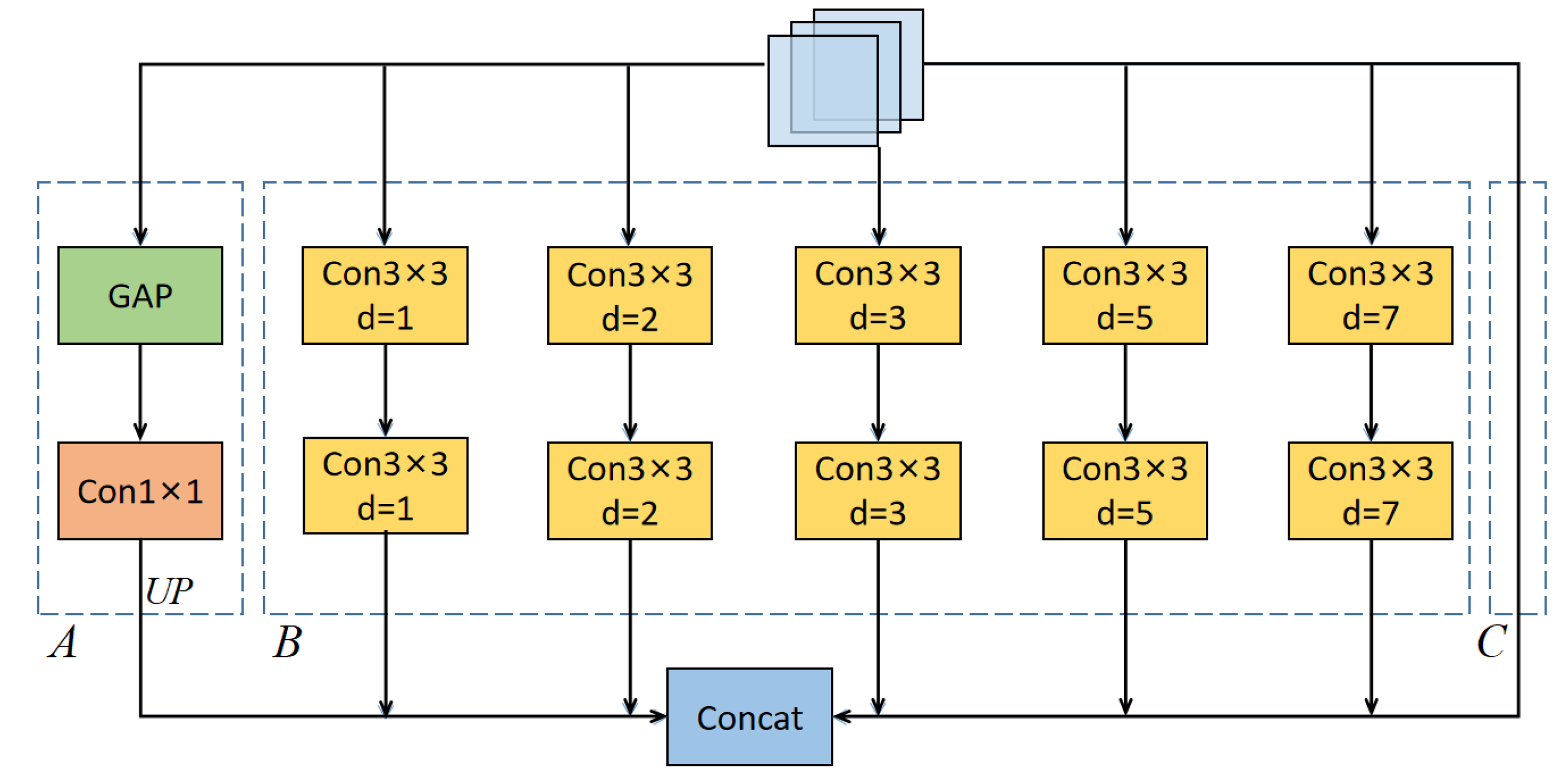
In remote sensing images, the scene is complex, and the size of the target is not same. In such cases, it is extremely difficult to extract target features only by a single scale. Therefore, multi-scale context information is indispensable to perform semantic segmentation. The difference in the size of the target and the complexity of the scene affect the feature extraction of the backbone network. In order to solve this problem, we propose a multi-scale context extraction module. It contains three main parts. The first part is responsible for extracting the global information; the second part uses atrous convolution to obtain information at several different scales; the third part is the feature map itself. The outputs of these three parts are concatenated at the end to form a multi-scale feature map. The structure of our multi-scale context extraction module is shown in Figure 1.

In the figure, yellow boxes represent $3\times 3$ atrous convolutions with dilatation rate $\mathrm{d}$. The stride of an atrous convolution is 1. GAP stands for global average pooling. Con1 × 1 represents a 1 × 1 convolution layer. UP denotes upsample operation. Concat means that features are concatenated according to the channel. The output results of the three parts are concatenated together to achieve a multi-scale context information extraction. Atrous convolutions with different dilatation rates can improve the receptive field and can extract features at different scales without introducing too many calculations.

2.1.1. Global Information Extraction

In image processing, convolution is the process of convolving an image with a kernel of specified size. This is usually performed to extract local features of the image. Although the receptive field of each convolution kernel will increase with the increase in the network depth, it is still not possible to obtain the global information. The extraction of global information is referred to generalization and integration of the features of the whole feature map, which can obtain global context information. In this part, i.e., part A in Figure 1, the features extracted from the last layer of the backbone network are subjected to global average pooling. The features obtained from each channel are averaged, and the number of channels is adjusted by a 1 × 1 convolution. Then, the global feature map is up-sampled. This part can be mathematically expressed as follows:

$$UP\left(C_{1\times 1}\left(GAP\left(X\right)\right)\right)$$

(1)

where, X represents the feature map extracted by the backbone network and $C_{1\times 1}$ represents a convolution layer.

2.1.2. Parallel Atrous Convolution Multi-Scale Context Extraction

Two layers of convolution operations at different scales can change the receptive field of the convolution kernel and can obtain context information at different scales. However, using multiple convolution kernels of different scales to extract multi-scale context information in the last feature map will increase the number of parameters as well as the computation steps. Inspired by the network structure of the DeepLab [33,34,35], a $3\times 3$ atrous convolution with different dilatation rate is used to substitute the conventional convolution. The main advantage is that it will obtain multi-scale context information without introducing too many parameters and computations. The dilatation rates of the atrous convolutions are 1, 2, 3, 5, and 7, respectively. This is equivalent to using the conventional convolution kernels of sizes 3, 5, 7, 11, and 15, respectively. The size of the training image is $512\times 512$ and the size of the feature map after feature extraction is $16\times 16$. In order to extract context information as much as possible, the maximum value of the dilatation rate is selected to be 7. When the dilatation rate of the atrous convolution is 5, it is equivalent to inserting four kernel elements between each element in a $3\times 3$ convolution kernel. The $3\times 3$ convolution is transformed into a $11\times 11$ convolution so as to enlarge the receptive field of each kernel element. Here, the strides of all $3\times 3$ atrous convolutions are 1. It is worth noting that although the $3\times 3$ convolution is transformed into an $11\times 11$ one, only the original $3\times 3$ kernel elements are used for calculations, that is to say that the total number of computations is not increased. Apart from that, the dilation rate $\mathrm{d}$ can be flexibly adjusted according to the image size. The maximum value of $\mathrm{d}$ is determined based on the size of the feature map extracted by the backbone network.

Assuming the feature map size is $m\times m$, the minimum and maximum values of $\mathrm{d}$ are 1 and $⌊(m-3)/2⌋+1$, respectively. For our experiments, the size of the feature map extracted by the backbone network is $16\times 16$, so the maximum d is 7. When the d is 1, 2, and 3, the neighboring pixels are considered in the feature extraction. When d is 5 and 7, the receptive field becomes larger so that more context information is considered in the feature extraction. In order to further increase nonlinearity of the model, we used batch normalization and a ReLU activation function after each convolution layer. Finally, all the outputs of this part are concatenated together. This second part of our multi-scale context extraction module, i.e., part B in Figure 1, can be expressed as follows:

$$\langle C_{3\times 3}^d\left(C_{3\times 3}^d\left(X\right)\right)\rangle ,\mathrm{d}=1,2,3,5,7$$

(2)

where, $\langle •\rangle$ represents feature concatenation, i.e., each feature is concatenated according to the channel and $C_{3\times 3}^d$ stands for a $3\times 3$ atrous convolution with a dilatation rate of $\mathrm{d}$.

In order to retain the original feature map, the input features extracted by the backbone network are directly combined with global context information and parallel multi-scale context information. In this way, we are able to extract the multi-scale context. The overall module is expressed as in Equation (3).

$$\langle UP\left(C_{1\times 1}\left(GAP\left(X\right)\right)\right)•C_{3\times 3}^d\left(C_{3\times 3}^d\left(X\right)\right)•X\rangle ,d=1,2,3,5,7$$

(3)

where, $C_{3\times 3}^d$ stands for a 3 × 3 atrous convolution with a dilation rate of $\mathrm{d}$ and $C_{1\times 1}$ is a 1 × 1 convolution layer.

2.2. Adaptive Fusion Module

As mentioned before, the scene in remote sensing images is complicated and the visual effects are similar for different categories due to the shooting angle. To alleviate this problem, the fusion of high- and low-level features to generate key features is essential. In semantic segmentation, the features extracted by the backbone network are usually distributed into different levels. The low-level features contain a lot of contour information whereas the high-level features contain rich semantic information [36]. In recent years, many methods were presented in the literature specifying the ways to fuse these high- and low-level features. FCN uses a skip-connection operation where the high-level abstract semantic information and the low-level fine semantic information are directly added according to corresponding channels to form new features. U-net [29] combines the semantic features of each layer extracted from the backbone network and the corresponding size features according to the channel to restore the resolution layer by layer. Most of these fusion methods use pixel-by-pixel addition or channel-by-channel concatenation. Despite of fusing high-level and low-level semantic information, these methods do not determine the channels with useful features and the channels with useless features. 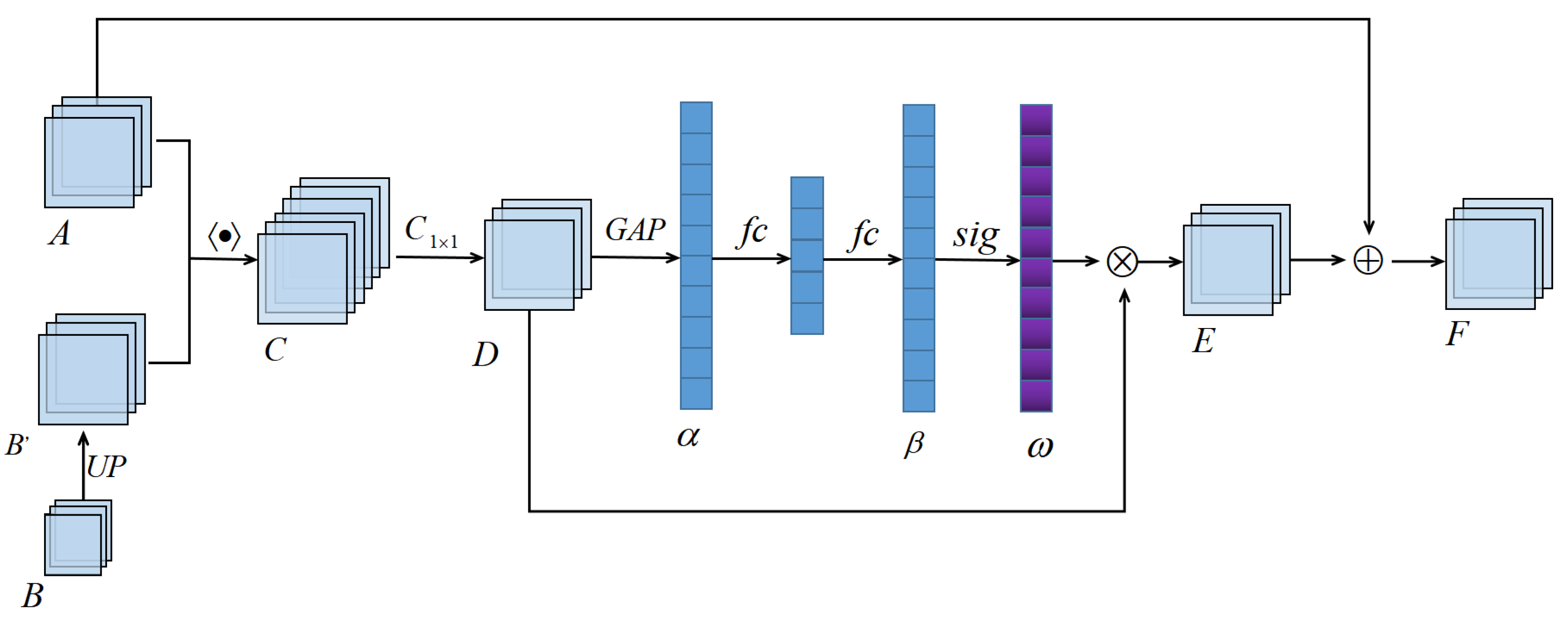Inspired by SENet [27], in this work we introduce a channel attention mechanism to high- and low-level semantic information fusion module and propose an adaptive fusion module to fuse the high- and low-level semantic features. Its structure is shown in Figure 2.

The upsampling of feature map B is accomplished via bilinear interpolation through which we can obtain a new feature map $B^{\prime }$ that is twice the size of B. The low-level semantic features A extracted from the backbone network and the features $B^{\prime }$ are concatenated to form a new feature C. The number of channels of C is the sum of the channels in $B^{\prime }$ and A. Next, the feature map D is generated from C through a $1\times 1$ convolution layer. D has half as many channels as C. The weight information $\alpha$ can be obtained using global average pooling for each channel of D. The weights $\beta$ can be generated from $\alpha$ via two full connected layers. The normalized weights $\omega$ are acquired from $\beta$ using a sigmoid function. Then, the weights $\omega$ are multiplied with D to get a new feature map E. Feature map E is readjusted using D on the channel according to its importance. E highlights features of useful channels and suppresses features of unwanted channels. Finally, the low-level feature map A is directly added to the feature map E to obtain the feature F which is the final fusion feature. This part can be expressed as:

$$sig(fc\left(GAP\left(C_{1\times 1}\left(\langle UP\left(X_1\right)•X_2\rangle \right)\right)\right)\ast C_{1\times 1}\left(\langle UP\left(X_1\right)•X_2\rangle \right))+X_2$$

(4)

where, $sig\left(\right)$ is the sigmoid activation function and $fc$ is the fully connected layer. UP denotes the upsample. $\langle •\rangle$ represents each feature is concatenated according to the channel. $X_1$ represents the high-level semantic features and $X_2$ represents the low-level semantic features. $C_{1\times 1}$ represents a 1 × 1 convolution layer.

2.3. Multi-Scale Adaptive Feature Fusion Network (MANet)

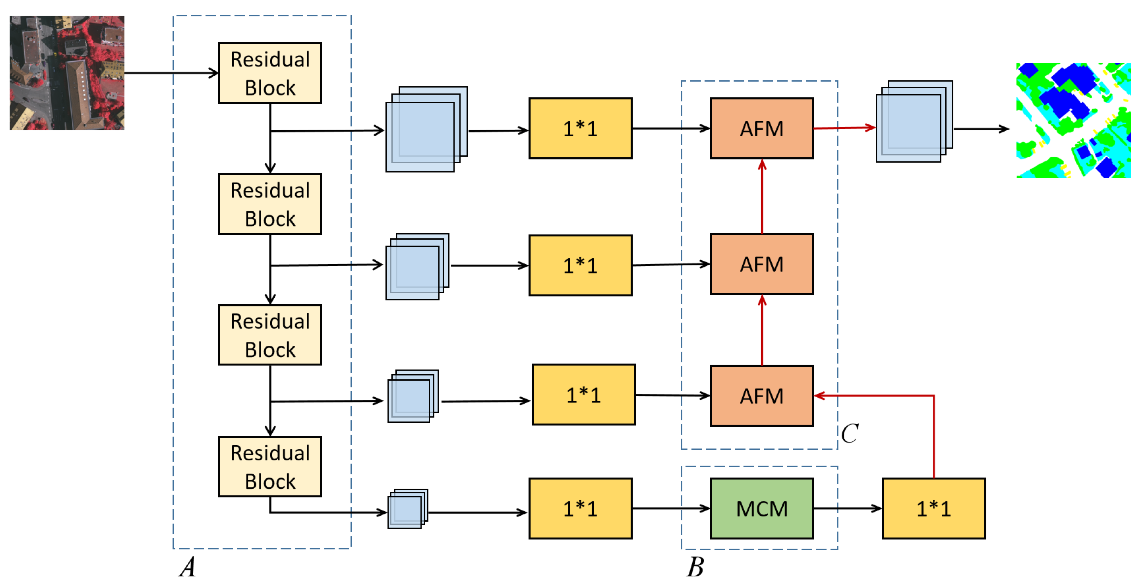
Based on the two modules above, we propose an end-to-end multi-scale adaptive feature fusion network. Its overall structure is shown in Figure 3.

The parts A, B, and C of our proposed MANet algorithm can be seen in Figure 3. As a reminder, part A is the backbone network, part B is a multi-scale context extraction module, and part C is a high- and low-level feature adaptive fusion module. The red arrow in the figure represents upsampling. The signifier ’1 * 1’ represents a $1\times 1$ convolution layer to change the number of channels. The multi-scale context extraction module (MCM) is the context extraction module that extracts the multi-scale context information to solve the problem associated with difference target sizes. The adaptive fusion module introduces channel attention to the fusion process of high-level and low-level layers. The efficient fusion of features can alleviate the problem of incorrect segmentation caused by similar features of similar categories.

In this work we have used ResNet101 as our backbone network to extract image features. Given an input image feed to the backbone network, it passes through four stages of the network, where each stage generates features with different sizes and channels. As the number of channels at each stage is different, a $1\times 1$ convolution is adopted to reduce the channels so as to have the same number of channels maintained at each stage’s output. The final stage features are fed to the context extraction module where the multi-scale context information is extracted and concatenated. This solves the problem of excessive target size differences in remote sensing images. The channels of the concatenated features are reduced by 1*1 to generate new features, which are up-sampled and fed to the adaptive fusion module. The adaptive fusion module fuses high-level and low-level semantic information efficiently and emphasize the useful features by learned weights. Later, the features extracted at each stage of the network are fused with the integrated features in a bottom-up manner by the adaptive fusion module. Through this we can get a feature map with 1/4th the size of the input image. Then, we adopt bilinear interpolation to restore the feature map to the same size as the input image. Finally, the output is sent to the classifier to receive the segmentation results.

In order or classify the output, We have used a softmax classifier [37] with our network. Softmax is a multi-class classifier that can calculate the probability of each category and the sum of the probabilities of all categories is 1. The classification of a pixel can be expressed as:

$$p_i=\frac{exp\left(X_i^l\right)}{{\sum }_{j=1}^{n}exp\left(X_j^l\right)}$$

(5)

where n is the total number of categories. $p_i$ represents the probability of a pixel l belongs to category i. Cross entropy loss function [38] has been adopted to represent the difference between the prediction and the label. Suppose that there is a training sample set $\{(x^{\left(1\right)},y^{\left(1\right)}),\dots ,(x^{\left(\mathrm{m}\right)},y^{\left(\mathrm{m}\right)})\}$ with m pixels, the cross-entropy loss function is:

$$L\left(W\right)=-\frac{1}{\mathrm{m}}\sum _{j=1}^{\mathrm{m}}\sum _{i=1}^n\mathrm{I}(y^j=i)\ast \log (\mathrm{P}(y_{}^{\left(j\right)}=i|x_{}^{\left(j\right)};W))$$

(6)

where $I(y^j=i)$ is an indicator function. The result is 1 when the prediction is equal to the label, and the result is 0 otherwise. The network can get a loss via forward propagation, and the back propagation algorithm can be adopted to transfer the loss from the back to the front to update network parameters [39]. In this paper, the stochastic gradient descent method is used to update the network parameters.

3. Experiment and Analysis

In order to verify the effectiveness of our proposed method, we have conducted various experiments using publicly available Potsdam and Vaihingen datasets. In this section, we first briefly describe the datasets and training settings, then present the experiments performed on the two datasets. To further verify the validity of our proposed method we have designed some ablation experiments that are presented at the end.

3.1. Datasets Description

The Potsdam and Vaihingen datasets are provided by the ISPRS II/4 committee for semantic segmentation [40]. These are well-known in the remote sensing community and contain images of the cities and their surroundings. They can be downloaded online from the following address: http://www2.isprs.org/commissions/comm3/wg4/data-request-form2.html. The images in the datasets have six common categories including impervious surface (white), building (blue), low vegetation (cyan), tree (green), car (yellow), and background (red). Sample images along with their corresponding labels from both these datasets are shown in the Figure 4.

Potsdam is a historic city in Germany, with large buildings and densely intertwined streets. The Potsdam dataset contains 38 images at a ground surface distance (GSD) of about 9 cm, including five channels of infrared, red, green, blue, and digital surface models (DSM) with a resolution of 6000 × 6000 pixels. For experiments, out of the available 38, we used 24 images for training and 14 images for testing. Note that we used ground truth with no eroded boundary labels in the experiments. On the other hand, Vaihingen is a village with small and scattered buildings. The Vaihingen dataset contains 3-band IRRG (infrared, red, and green) image data, corresponding DSM, and a normalized digital surface model (NDSM) data [41]. At a GSD of about 9 cm, there are 33 images of about 2500 × 2000 pixels. We used 16 of the images for training and 17 of the images for testing. Similar to the other dataset, we have used the ground truth with no eroded boundary labels in the experiments.

Due to GPU memory limitations we needed to change the size of the images in the datasets. This can be done either by reducing the resolution or by cropping the image. However, by reducing the resolution, we will lose useful information in the image. For this reason, we reduced the size of each image and its corresponding label by cropping it to a size of 512 × 512 pixels with a 100 pixel overlap. The test images are mirror-filled and cropped to a size of 512 × 512 pixels with an overlap of 256 pixels and the final prediction results were stitched. The amount of data used can significantly affect the performance of the model. Sufficient data can prevent the model from overfitting and improve the robustness of the model. Data augmentation is an efficient way to solve the problem with data volume. In terms of spatial position, we employed horizontal and vertical rotation and random scale rotation. Random changes in brightness, saturation, and contrast were adopted in color. It is worth noting that the size of the images in the Vaihingen dataset is too small. The original training image is scaled to 0.5, 0.75, 1.25, and 1.5 times and cropped according to the above method.

3.2. Compared State-of-the-Art Methods

In order to better evaluate the network performance of our proposed MANet, we have compared its performance with FCN8s [28], U-net [29], UZ1 [42], Light-weight RefineNet [43], DeepLabv3+ [31], and APPD [32] methods. FCN is a well-known method in semantic segmentation. It is further divided into FCN32s, FCN16s, and FCN8s based on the type of skip-connections. In this work, we chose FCN8s with fine edge segmentation for comparison. UZ1 is a CNN-based encoder–decoder model that employs a deconvolution layer as a decoder. U-net employs high-level and low-level feature fusion. It simply stitches the features from channels together to form more features. Light-weight RefineNet is a lightweight and efficient network that uses a chained residual pooling module and a layer-by-layer fusion module for segmentation. DeepLabv3+ uses a spatial pyramid to obtain multi-scale semantic information, and adopts the structure of encoding and decoding to refine the segmentation results. APPD combines the advantages of both deeplabv3+ and U-net, considering the strategies of multi-scale context information and multi-scale feature fusion. It also uses post-processing based on super pixel.

3.3. Training Details

The proposed method was implemented using the PyTorch library. The size of the images used for both training and testing was 512 × 512. ResNet101 pre-trained on ImageNet was used for our backbone network. The MANet was trained on two Titan 1080 GPUs, each with 12 GB of memory. The total batch size was set to 12. Cross entropy was used as a loss function to update network parameters. Stochastic gradient descent with momentum was applied to optimize the network. The momentum and weight decay were set to 0.99 and 0.0005, respectively. We adjusted the learning rate according to the training epochs. The initial learning rate was set to 0.001. A new learning rate was set every 30 epochs, as shown in

Table 1. Setting of the learning rate.

Epoch	1–30	31–60	61–90	91–120	121–150	151–180
LearningRate	0.001	0.0005	0.0001	0.00005	0.00001	0.000005

. It is worth noting that the experimental settings of all the compared algorithms are the same as the proposed MANet.

3.4. Metrics

In order to comprehensively evaluate the performance of different networks, we chose overall accuracy (OA), F1, precision, and recall [44] as our evaluation metrics. They are formulated as in the below equations.

$$\mathrm{OA}=\frac{\mathrm{TP}+\mathrm{TN}}{\mathrm{TP}+\mathrm{TN}+\mathrm{FP}+\mathrm{FN}}$$

(7)

$$\mathrm{precision}=\frac{\mathrm{TP}}{\mathrm{TP}+\mathrm{FP}}$$

(8)

$$\mathrm{recall}=\frac{\mathrm{TP}}{\mathrm{TP}+\mathrm{FN}}$$

(9)

$$\mathrm{F}1=2\times \frac{\mathrm{precision}\times \mathrm{recall}}{\mathrm{precision}+\mathrm{recall}}$$

(10)

where TP is the number of true positives and TN is the number of true negatives. FP is the number of false positives and FN is the number of false negatives. It is worth noting that the overall accuracy is the accuracy of all categories including background. In addition, for the task of pixel classification, when the categories are not balanced, precision and recall are used for prediction. To this end, we draw a precision-recall (PR) curve to measure the relationship between the precision and the recall of each category. Technically, we first obtain the model’s score map in each category and select a series of thresholds between 0 and 1. Next, we obtain the numbers of TP, FP, and FN according to the thresholds. Then calculate the precision and recall under different thresholds. Finally, draw the PR curve with recall as the horizontal axis and precision as the vertical axis.

3.5. Experimental Results and Analysis

3.5.1. Experiments on the Potsdam Dataset

The first set of experiments were performed on the Potsdam dataset. For all the compared models, we computed the F1 for each category as well as the average of other metrics. The results are summarized in

Table 2. The F1 for each category and the average of four metrics for all seven models on the Potsdam dataset.

Models	Imp Sur	Building	Low Veg	Tree	Car	F1 Ave	Pre Ave	Recall Ave	OA
FCN8s [28]	0.864	0.927	0.806	0.833	0.662	0.818	0.829	0.811	0.846
U-net [29]	0.881	0.922	0.813	0.838	0.869	0.865	0.862	0.868	0.853
UZ1 [42]	0.869	0.893	0.825	0.835	0.887	0.862	0.861	0.864	0.846
DeepLabv3+ [31]	0.905	0.953	0.845	0.857	0.896	0.891	0.889	0.893	0.883
LWRefineNet [43]	0.909	0.953	0.846	0.849	0.896	0.890	0.890	0.891	0.884
APPD [32]	0.910	0.958	0.848	0.853	0.894	0.893	0.898	0.889	0.884
MANet	0.916	0.961	0.859	0.871	0.914	0.904	0.900	0.908	0.894

.

It can be seen from the results that the proposed MANet achieved a result of 89.4% in OA and 90.4% in the F1 average. In comparison with APPD, it showed an improvement of 1% and 1.1% in OA F1 average, respectively. MANet achieved 0.6%, 0.3%, 1.1%, 1.8%, and 2% improvements, respectively, in the F1 of each category compared with APPD. Although the compared six methods considered the fusion of high-level and low-level features, they did not take into account the weights of the feature fusion. On the other hand, our proposed method can readjust the fused features by learning the weights (of the fused features). Because of this, our method can better distinguish categories and reduce false positives. Areas of low vegetation and trees are very similar and are very prone to causing an incorrect segmentation. Nevertheless, our method showed better performance in these two categories with an improved F1 score of 1.1% and 1.8%, respectively. These results clearly demonstrate the effectiveness of our adaptive fusion module. In the dataset, the car is a small target compared to several other categories, and the impervious surface is a large target. From Table 2, it can be seen that for these two categories, the F1 values increased by 0.6% and 2%, respectively. This shows that our proposed multi-scale context extraction module can solve the problem associated with variable target sizes, i.e., when the difference between two target size’s is too large. Based on these two modules, the network can extract features more accurately and fuse high-level and low-level semantic features efficiently, thereby improving the overall segmentation performance.

In order to make a comprehensive comparison of each model, when data are not balanced, precision and recall are important indicators for evaluating segmentation performance. The PR curve can clearly show the relationship between precision and recall. The PR curves for each category of each model on the Potsdam dataset are shown in Figure 5. It can be seen that for all categories MANet achieved better results even when the data is unevenly distributed in the categories.

In order to compare the segmentation performance of our proposed MANet more intuitively and clearly, the visualization results of FCN8s, U-net, UZ1, Light-weight RefineNet, DeepLabv3+, APPD, and MANet are shown in Figure 6. In the figure, the first and the third rows show the image, ground truth, and the predictions from all seven methods. The second and the fourth rows are the predicted segmentation results corresponding to a small region in the graph, marked with a red box. It can be noticed that the two similar categories of low vegetation and tree in the second row cannot be distinguished well by other models. However, MANet demonstrated a smoother result for these challenging categories. All these results clearly demonstrate the efficiency of our method for semantic segmentation.

3.5.2. Experiments on the Vaihingen Dataset

Similar tests were performed on the Vaihingen dataset. The F1 for each category and the average of four metrics for all the seven models are summarized in

Table 3. The F1 for each category and the average of four metrics of the seven models on the Vaihingen dataset.

Models	Imp Sur	Building	Low Veg	Tree	Car	F1 Ave	Pre Ave	Recall Ave	OA
FCN8s [28]	0.838	0.890	0.753	0.822	0.326	0.726	0.781	0.710	0.823
U-net [29]	0.838	0.878	0.749	0.847	0.311	0.725	0.780	0.710	0.823
UZ1 [42]	0.872	0.902	0.788	0.863	0.728	0.830	0.838	0.825	0.855
DeepLabv3+ [31]	0.891	0.935	0.792	0.866	0.721	0.841	0.860	0.830	0.870
LWRefineNet [43]	0.887	0.935	0.807	0.866	0.747	0.848	0.853	0.844	0.872
APPD [32]	0.889	0.936	0.798	0.867	0.760	0.850	0.855	0.835	0.872
MANet	0.902	0.941	0.809	0.870	0.812	0.867	0.870	0.867	0.882

.

From the obtained results, the OA of MANet on the Vaihingen dataset is 88.2%, and the average of F1 is 86.7%, which is 1.7% and 1% higher, respectively, than its nearest competitor method APPD. Even though the amount of Vaihingen data is comparatively smaller than that of the Potsdam data, our method still managed to obtain better performance. Especially for the car category, where it achieved a 5.2% higher F1 than the APPD. Because the cars occupy a small proportion of pixels in the total training images and are occluded by buildings and trees, it is difficult for the other models to extract corresponding features for correct pixel classification. With our proposed MANet, the features of different scale targets are extracted by a multi-scale context extraction module, and the adaptive fusion module fuses the high-level and low-level semantic information adaptively. Due to this, even when the targets occupy small areas in the images, they can be extracted and fused to form valid features for correct segmentation. Even though the categories are not evenly distributed, the average of precision and recall in all categories are increased by 1.5% and 3.2%, respectively.

In addition, the PR curves of each model in each category of the Vaihingen dataset are shown in Figure 7. Similar to before, our proposed MANet demonstrated better segmentation performance than the other six models. Visual comparison results with this dataset are shown in Figure 8. It can be seen from the second row that the FCN8s and UZ1 methods show very degraded performance for low vegetation and trees. None of the six comparison methods segmented the car occluded by a tree. From the fourth row, it can be seen that the segmentation of the two similar categories of tree and low vegetation is prone to cause confusion. Besides, the segmentation results of UZ1 and U-net on buildings are incomplete. Even in this case, from the results shown in first and third rows, our proposed method showed a smoother performance.

3.6. Ablation Experiment

We decomposed and combined the proposed network to verify the effeteness of each module using F1 and OA metrics. This experiment used the Potsdam dataset. Firstly, the ResNet101 model was used as the basic network (Res101), and the last output feature map was up-sampled and passed to a classifier for segmentation. First, Res101+MCM were employed to verify the effectiveness of the context extraction module. The feature map extracted by Res101 was fed into the multi-scale context extraction module to obtain a new feature map. This was then up-sampled for the prediction. Next, the Res101 + adaptive fusion module (AFM) were adopted to verify the effectiveness of feature fusion. The feature map extracted by each stage of the backbone network was fed into the adaptive fusion module, and the output was up-sampled for the prediction. Finally, we integrated the two modules together, Res101+MCM+AFM. The experimental results are summarized in

Table 4. Comparison of each module on the metrics of F1 and overall accuracy (OA).

Models	Imp Sur	Building	Low Veg	Tree	Car	mean F1	OA
Res101	0.882	0.932	0.805	0.817	0.789	0.845	0.850
Res101+CMM	0.893	0.937	0.820	0.853	0.796	0.860	0.862
Res101+AFM	0.904	0.951	0.844	0.862	0.909	0.894	0.883
Res101+CMM+AFM	0.916	0.961	0.859	0.871	0.914	0.904	0.894

.

We can observe that the “Res101+CMM” yields a result of 86.2% in OA and 86% in mean F1, which is 1.2% and 1.5% more than that of the “Res101”. Multi-scale context extraction can further extract multi-scale features of the feature map from the backbone network, which solves the problem associated with greater target size differences. Besides, “Res101+AFM” outperforms the “Res101” by 3.3% in OA and 4.9% in mean F1. Each layer features extracted by the backbone network are rich in semantic information and the reasonable and efficient fusion of these features can improve the segmentation performance. Our model introduces channel attention with the fusion process that readjusts the features through learned weights. Furthermore, when we utilize the integration of two modules together, the performance is further boosted up. Compared with the Res101, “Res101+AMM+CFM” segmentation performance is improved by by 4.4% in OA and 5.9% in mean F1. The multi-scale context extraction module is employed to extract multi-scale context information. The adaptive fusion module can efficiently fuse the features to alleviate the misclassification of similar categories. The results of ablation experiments show that both our proposed multi-scale context information extraction and adaptive fusion modules can significantly improve the performance of remote sensing image semantic segmentation.

4. Discussion

4.1. Model Complexity

In this subsection, we analyze the computational complexity of the MANet. Computational complexity includes the total number of floating point operations (FLOPs), number of network parameters and average test time for each image of size 512 × 512 pixels on two Titan 1080 GPUs with 12G RAM. The results are shown in

Table 5. The computation complexity of MANet and six other compared methods.

Models	Input Size	Parameters (M)	Flop (GFLOPs)	Test Time (ms)
FCN8s [28]	512 × 512	512	189	27
U-net [29]	512 × 512	27	3.5	10
UZ1 [42]	512 × 512	22	221	22
DeepLabv3+ [31]	512 × 512	226	89	19
LWRefineNet [43]	512 × 512	176	51	16
APPD [32]	512 × 512	229	91	20
MANet	512 × 512	424	63	20

. The computational scale of the MANet is reduced to a certain degree compared to FCN8s, UZ1, DeepLabv3+, and APPD. It is slightly larger than that of the LWRefineNet. However, the total number of parameters in the MANet is more than other methods. Due to multi-scale context extraction module in MANet, a lot of parallel convolutions make the total number of parameters large. In the case of average test time, our proposed method is at the same level with compared models.

4.2. Experiments on Small-Scale Dataset

To verify the performance of our model on small dataset, the proposed method was tested on a set of 20 multi-spectral Very-High-Resolution (VHR) images acquired over the city of Zurich by the QuickBird satellite in 2002 [45]. The average image size is 1000 × 1150 pixels and consists of four channels that span the near infrared to visible spectrum (NIR-R-G-B). The spatial resolution of the pan-sharpened image is 0.61 m/pixel. The images in the Zurich dataset are divided into eight categories including Road, Building, Tree, Grass, Bare Soil, Water, Rail, and Pool. An example along with the urban class legend is shown in Figure 9. Note that white background is not considered a separate class.

zh1–zh13 were used for training and zh14–zh20 were used for testing in Zurich dataset. The size of each image and its corresponding label by cropping it was reduced to a size of 512 × 512 pixels with an overlap of 256 pixels. The original training images were scaled to 0.5,0.75, 1.25, and 1.5 times and cropped according to the above method. The test images were mirror-filled and cropped to a size of 512 × 512 pixels with an overlap of 256 pixels. The experimental setup was the same as the training details in Section 3.3. The F1 for each category of MANet and the results of the six compared algorithms is obtained and shown in

Table 6. The F1 for each category of MANet and six other compared algorithms on the Zurich dataset.

Models	Road	Building	Tree	Grass	Bare Soil	Water	Rail	Pool
FCN8s [28]	0.517	0.586	609	0.669	0.587	0.868	0.023	0.622
U-net [29]	0.698	0.777	0.665	0.729	0.558	0.946	0.023	0.859
UZ1 [42]	0.693	0.784	0.695	0.756	0.510	0.946	0.316	0.813
DeepLabv3+ [31]	0.709	0.809	0.687	0.786	0.619	0.948	0.224	0.839
LWRefineNet [43]	0.711	0.812	0.731	0.803	0.607	0.941	0.150	0.814
APPD [32]	0.702	0.813	0.740	0.809	0.637	0.947	0.391	0.799
MANet	0.711	0.819	0.732	0.791	0.669	0.951	0.262	0.867

.

As can be seen from Table 6, MANet is superior to the other models in the categories of Road, Building, Bare Soil, Water, and Pool, which achieves 0.9%, 0.6%, 3.2%, 0.4%, and 6.8% improvements, respectively, in F1 of those category compared with APPD. However, F1 in the three categories of Trees, Grass, and Rail is lower than the compared algorithms. The two categories of grass and trees are similar in the Zurich dataset. Insufficient training data affects our model to extract corresponding features, making it difficult to correctly classify its pixels. Therefore, it can be seen from Table 6 that the proposed method has improved on small data, but the effect is not obvious.

5. Conclusions

In this paper, we propose a multi-scale adaptive feature fusion network for semantic segmentation in remote sensing images, namely MANet. The MANet uses encoding–decoding architecture with multi-scale context extraction and adaptive fusion modules. It uses ResNet101 as the backbone network for encoding and multi-scale context extraction and adaptive fusion modules for decoding. The multi-scale context extraction module is composed of two parallel layers of atrous convolutions with different dilatation rates, global information, and its own features. It extracts multi-scale context information to solve the problem of high differences in target sizes in remote sensing images. The adaptive fusion module introduces the channel attention mechanism into high-level and low-level semantic features in the fusion process, which adjust the fused features by the learned weights. By integrating these two modules together, the overall segmentation performance is significantly boosted up.

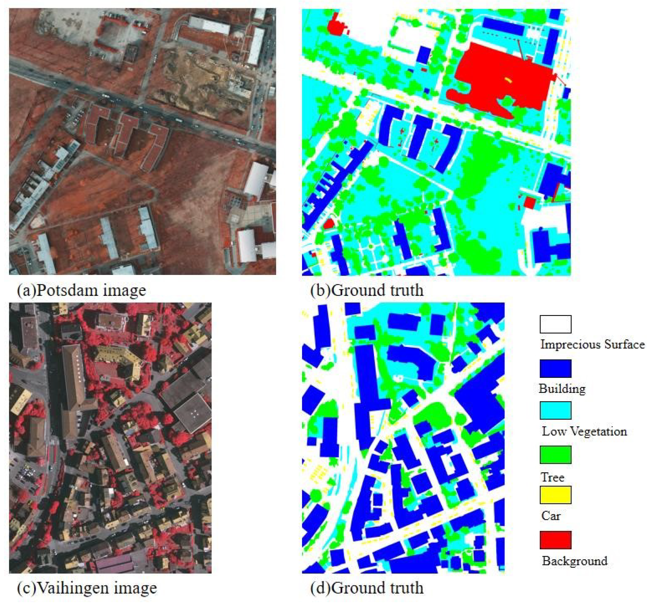
We have evaluated the proposed MANet on two publicly available benchmark datasets, Potsdam and Vaihingen datasets. With the Potsdam dataset, MANet achieved a result of 89.4% in overall accuracy and 90.4% in the average of F1 which brings 1% and 1.1% improvement in OA and the average of F1 compared with APPD, respectively. On the Vaihingen dataset, the OA of MANet is 88.2% and the average of F1 is 86.7%. Experimental results show that our proposed MANet outperforms other state-of-the-art models on both datasets, in terms of overall accuracy and F1. In ablation experiments, the performance of the “Res101+AMM+CFM” is increased over “Res101” by 4.4% in OA and 5.9% in mean F1. The ablation experiments further verify the effectiveness of the proposed module in semantic segmentation of remote sensing images. It is worth noting that the available information of the corresponding DSM and NDSM data in the Potsdam dataset is not used to assist in segmentation. Nevertheless, the parameter size of our proposed method is large. In the future, we aim to reduce this count. Moreover, semantic segmentation of remote sensing images belongs to supervised learning. The data labeling workload of semantic segmentation is huge, especially for remote sensing images. Semantic segmentation based on semi-supervised and unsupervised learning is therefore an important future research direction.

References

1. Zhang, L.; Zhang, L.; Du, B. Deep learning for remote sensing data: A technical tutorial on the state of the art. IEEE Geosci. Remote Sens. Mag. 2016, 4, 22–40. [Google Scholar] [CrossRef]
2. Singh, V.; Misra, A.K. Detection of plant leaf diseases using image segmentation and soft computing techniques. Inf. Process. Agric. 2017, 4, 41–49. [Google Scholar] [CrossRef] [Green Version]
3. Wen, D.; Huang, X.; Liu, H.; Liao, W.; Zhang, L. Semantic classification of urban trees using very high resolution satellite imagery. IEEE J. Sel. Top. Appl. Earth Obs. Remote Sens. 2017, 10, 1413–1424. [Google Scholar] [CrossRef]
4. Shi, Y.; Qi, Z.; Liu, X.; Niu, N.; Zhang, H. Urban Land Use and Land Cover Classification Using Multisource Remote Sensing Images and Social Media Data. Remote Sens. 2019, 11, 2719. [Google Scholar] [CrossRef] [Green Version]
5. Matikainen, L.; Karila, K. Segment-based land cover mapping of a suburban area—Comparison of high-resolution remotely sensed datasets using classification trees and test field points. Remote Sens. 2011, 3, 1777–1804. [Google Scholar] [CrossRef] [Green Version]
6. Xu, S.; Pan, X.; Li, E.; Wu, B.; Bu, S.; Dong, W.; Xiang, S.; Zhang, X. Automatic building rooftop extraction from aerial images via hierarchical rgb-d priors. IEEE Trans. Geosci. Remote Sens. 2018, 56, 7369–7387. [Google Scholar] [CrossRef]
7. Liu, W.; Yang, M.; Xie, M.; Guo, Z.; Li, E.; Zhang, L.; Pei, T.; Wang, D. Accurate Building Extraction from Fused DSM and UAV Images Using a Chain Fully Convolutional Neural Network. Remote Sens. 2019, 11, 2912. [Google Scholar] [CrossRef] [Green Version]
8. Xu, Y.; Xie, Z.; Feng, Y.; Chen, Z. Road extraction from high-resolution remote sensing imagery using deep learning. Remote Sens. 2018, 10, 1461. [Google Scholar] [CrossRef] [Green Version]
9. Shrestha, S.; Vanneschi, L. Improved fully convolutional network with conditional random fields for building extraction. Remote Sens. 2018, 10, 1135. [Google Scholar] [CrossRef] [Green Version]
10. Cheng, G.; Han, J.; Lu, X. Remote sensing image scene classification: Benchmark and state of the art. Proc. IEEE 2017, 105, 1865–1883. [Google Scholar] [CrossRef] [Green Version]
11. Zhao, C.; Sun, L.; Stolkin, R. A fully end-to-end deep learning approach for real-time simultaneous 3D reconstruction and material recognition. In Proceedings of the 2017 18th International Conference on Advanced Robotics (ICAR), Hong Kong, China, 10–12 July 2017; pp. 75–82. [Google Scholar]
12. Sun, L.; Zhao, C.; Yan, Z.; Liu, P.; Duckett, T.; Stolkin, R. A novel weakly-supervised approach for RGB-D-based nuclear waste object detection. IEEE Sensors J. 2018, 19, 3487–3500. [Google Scholar] [CrossRef] [Green Version]
13. Guo, S.; Jin, Q.; Wang, H.; Wang, X.; Wang, Y.; Xiang, S. Learnable gated convolutional neural network for semantic segmentation in remote-sensing images. Remote Sens. 2019, 11, 1922. [Google Scholar] [CrossRef] [Green Version]
14. Dalal, N.; Triggs, B. Histograms of oriented gradients for human detection. In Proceedings of the 2005 IEEE Computer Society Conference on Computer Vision and Pattern Recognition (CVPR’05), San Diego, CA, USA, 20–25 June 2005; Volume 1, pp. 886–893. [Google Scholar]
15. Lowe, D.G. Distinctive image features from scale-invariant keypoints. Int. J. Comput. Vis. 2004, 60, 91–110. [Google Scholar] [CrossRef]
16. Kahaki, S.M.M.; Nordin, M.J.; Ashtari, A.H.; Zahra, S.J. Deformation invariant image matching based on dissimilarity of spatial features. Neurocomputing 2016, 175, 1009–1018. [Google Scholar] [CrossRef]
17. Shui, P.L.; Zhang, W.C. Corner detection and classification using anisotropic directional derivative representations. IEEE Trans. Image Process. 2013, 22, 3204–3218. [Google Scholar] [CrossRef] [PubMed]
18. Kahaki, S.M.M.; Nordin, M.J.; Ashtari, A.H. Contour-based corner detection and classification by using mean projection transform. Sensors 2014, 14, 4126–4143. [Google Scholar] [CrossRef] [PubMed] [Green Version]
19. Inglada, J. Automatic recognition of man-made objects in high resolution optical remote sensing images by SVM classification of geometric image features. ISPRS J. Photogramm. Remote Sens. 2007, 62, 236–248. [Google Scholar] [CrossRef]
20. Wright, R.E. Logistic regression. In Reading and Understanding Multivariate Statistics; American Psychological Association: Washington, DC, USA, 1995; Chapter 7; pp. 217–244. [Google Scholar]
21. Belgiu, M.; Drăguţ, L. Random forest in remote sensing: A review of applications and future directions. ISPRS J. Photogramm. Remote Sens. 2016, 114, 24–31. [Google Scholar] [CrossRef]
22. Liu, Y.; Piramanayagam, S.; Monteiro, S.T.; Saber, E. Dense semantic labeling of very-high-resolution aerial imagery and lidar with fully-convolutional neural networks and higher-order CRFs. In Proceedings of the IEEE Conference on Computer Vision and Pattern Recognition Workshops, Honolulu, HI, USA, 21 July–26 July 2017; pp. 76–85. [Google Scholar]
23. Simonyan, K.; Zisserman, A. Very deep convolutional networks for large-scale image recognition. arXiv 2014, arXiv:1409.1556. [Google Scholar]
24. He, K.; Zhang, X.; Ren, S.; Sun, J. Deep residual learning for image recognition. In Proceedings of the IEEE Conference on Computer Vision and Pattern Recognition, Las Vegas, NV, USA, 27–30 June 2016; pp. 770–778. [Google Scholar]
25. Xie, S.; Girshick, R.; Dollár, P.; Tu, Z.; He, K. Aggregated residual transformations for deep neural networks. In Proceedings of the IEEE Conference on Computer Vision and Pattern Recognition, Honolulu, HI, USA, 21 July–26 July 2017; pp. 1492–1500. [Google Scholar]
26. Huang, G.; Liu, Z.; Van Der Maaten, L.; Weinberger, K.Q. Densely connected convolutional networks. In Proceedings of the IEEE Conference on Computer Vision and Pattern Recognition, Honolulu, HI, USA, 21 July–26 July 2017; pp. 4700–4708. [Google Scholar]
27. Hu, J.; Shen, L.; Sun, G. Squeeze-and-excitation networks. In Proceedings of the IEEE Conference on Computer Vision and Pattern Recognition, Salt Lake City, UT, USA, 18–23 June 2018; pp. 7132–7141. [Google Scholar]
28. Long, J.; Shelhamer, E.; Darrell, T. Fully convolutional networks for semantic segmentation. In Proceedings of the IEEE Conference on Computer Vision and Pattern Recognition, Boston, MA, USA, 8–10 June 2015; pp. 3431–3440. [Google Scholar]
29. Ronneberger, O.; Fischer, P.; Brox, T. U-net: Convolutional networks for biomedical image segmentation. In Proceedings of the International Conference on Medical Image Computing and Computer-Assisted Intervention, Munich, Germany, 5–9 October 2015; Springer: Berlin/Heidelberg, Germany, 2015; pp. 234–241. [Google Scholar]
30. Zhao, H.; Shi, J.; Qi, X.; Wang, X.; Jia, J. Pyramid scene parsing network. In Proceedings of the IEEE Conference on Computer Vision and Pattern Recognition, Honolulu, HI, USA, 21 July–26 July 2017; pp. 2881–2890. [Google Scholar]
31. Chen, L.C.; Zhu, Y.; Papandreou, G.; Schroff, F.; Adam, H. Encoder-decoder with atrous separable convolution for semantic image segmentation. In Proceedings of the European Conference on Computer Vision (ECCV), Munich, Germany, 8–14 September 2018; pp. 801–818. [Google Scholar]
32. Wang, Y.; Liang, B.; Ding, M.; Li, J. Dense Semantic Labeling with Atrous Spatial Pyramid Pooling and Decoder for High-Resolution Remote Sensing Imagery. Remote Sens. 2019, 11, 20. [Google Scholar] [CrossRef] [Green Version]
33. Chen, L.C.; Papandreou, G.; Kokkinos, I.; Murphy, K.; Yuille, A.L. Semantic image segmentation with deep convolutional nets and fully connected crfs. arXiv 2014, arXiv:1412.7062. [Google Scholar]
34. Chen, L.C.; Papandreou, G.; Kokkinos, I.; Murphy, K.; Yuille, A.L. Deeplab: Semantic image segmentation with deep convolutional nets, atrous convolution, and fully connected crfs. IEEE Trans. Pattern Anal. Mach. Intell. 2017, 40, 834–848. [Google Scholar] [CrossRef] [PubMed]
35. Chen, L.C.; Papandreou, G.; Schroff, F.; Adam, H. Rethinking atrous convolution for semantic image segmentation. arXiv 2017, arXiv:1706.05587. [Google Scholar]
36. Lin, T.Y.; Dollár, P.; Girshick, R.; He, K.; Hariharan, B.; Belongie, S. Feature pyramid networks for object detection. In Proceedings of the IEEE Conference on Computer Vision and Pattern Recognition, Honolulu, HI, USA, 21 July–26 July 2017; pp. 2117–2125. [Google Scholar]
37. LeCun, Y.; Bottou, L.; Bengio, Y.; Haffner, P.; others. Gradient-based learning applied to document recognition. Proc. IEEE 1998, 86, 2278–2324. [Google Scholar] [CrossRef] [Green Version]
38. Zeiler, M.D.; Fergus, R. Visualizing and understanding convolutional networks. In Proceedings of the European Conference on Computer Vision, Zurich, Switzerland, 6–12 September 2014; Springer: Berlin/Heidelberg, Germany, 2014; pp. 818–833. [Google Scholar]
39. Rumelhart, D.E.; Hinton, G.E.; Williams, R.J. Learning representations by back-propagating errors. Nature 1986, 323, 533–536. [Google Scholar] [CrossRef]
40. Konecny, G. The International Society for Photogrammetry and Remote Sensing (ISPRS) study on the status of mapping in the world. In International Workshop on “Global Geospatial Information”; Citeseer: Novosibirsk, Russian, 2013; pp. 4–24. [Google Scholar]
41. Cheng, W.; Yang, W.; Wang, M.; Wang, G.; Chen, J. Context Aggregation Network for Semantic Labeling in Aerial Images. Remote Sens. 2019, 11, 1158. [Google Scholar] [CrossRef] [Green Version]
42. Volpi, M.; Tuia, D. Dense semantic labeling of subdecimeter resolution images with convolutional neural networks. IEEE Trans. Geosci. Remote Sens. 2016, 55, 881–893. [Google Scholar] [CrossRef] [Green Version]
43. Nekrasov, V.; Dharmasiri, T.; Spek, A.; Drummond, T.; Shen, C.; Reid, I. Real-time joint semantic segmentation and depth estimation using asymmetric annotations. In Proceedings of the 2019 International Conference on Robotics and Automation (ICRA), Montreal, QC, Canada, 20–24 May 2019; pp. 7101–7107. [Google Scholar]
44. Kahaki, S.M.M.; Nordin, M.J.; Ashtari, A.H.; Zahra, S.J. Invariant feature matching for image registration application based on new dissimilarity of spatial features. PLoS ONE 2016, 11, e0149710. [Google Scholar]
45. Volpi, M.; Ferrari, V. Semantic segmentation of urban scenes by learning local class interactions. In Proceedings of the IEEE Conference on Computer Vision and Pattern Recognition Workshops, Boston, MA, USA, 7–12 June 2015; pp. 1–9. [Google Scholar]
Figure 1. The structure of our proposed multi-scale context extraction module. It contains three parts namely A, B, and C. Part A extracts global information. Part B is the parallel connection of atrous convolutions with different dilatation rate. Part C is the feature map itself. GAP stands for global average pooling. Con 1 × 1 represents a 1 × 1 convolution layer. UP denotes upsample operation. Concat means that the features are concatenated according to channel.
Remotesensing 12 00872 g001
Figure 2. Structure of the adaptive fusion module. A is a low-level feature map. B is a high-level feature map. B’ is a feature map obtained by B. C is a feature map of A and B’ combined by channel. D is a feature map of the channel changed by C. E is the feature map adjusted with channel weights. F is the final fusion feature map.
Remotesensing 12 00872 g002
Figure 3. The overall structure of the proposed multi-scale adaptive feature fusion network (MANet). Part A is the backbone network. Part B is a multi-scale context extraction module. Part C is a high- level and low-level feature adaptive fusion module.
Remotesensing 12 00872 g003
Figure 4. Images of the Potsdam and the Vaihingen dataset and their corresponding labels.
Remotesensing 12 00872 g004
Figure 5. Precision-recall (PR) curves for each category of the seven models on the Potsdam dataset.
Remotesensing 12 00872 g005
Figure 6. Visual comparison of seven models on the Potsdam dataset.
Remotesensing 12 00872 g006
Figure 7. PR curves for each category of the seven models on the Vaihingen dataset.
Remotesensing 12 00872 g007
Figure 8. Visual comparison of seven models on the Vaihingen dataset.
Remotesensing 12 00872 g008
Figure 9. Example from the Zurich dataset.
Remotesensing 12 00872 g009