1. Introduction
This study investigates the seasonal and interannual variations of satellite-measured sea surface salinity (SSS) in the Hudson Bay (HB) in the context of HB freshwater contents from river discharge, sea ice melt/freeze, and surface freshwater forcing (i.e., precipitation minus evaporation). Our main objective is to explore the potential use of satellite SSS in monitoring the HB freshwater cycle, despite the large uncertainty of SSS in polar region (~ 1 psu poleward of 50°) [
1,
2,
3]. Our secondary objective is to use the semi-enclosed environment of HB as a testbed to identify the limitations of the L-band SSS measurements and to improve satellite SSS retrieval algorithm.
The significance of HB is evident in its role as a recipient as well as a driver in global climate change [
4]. Located at the southern margin of the Arctic Circle, HB links the Arctic Ocean and subarctic North Atlantic Ocean through two main gateways: the Foxe Basin and the Hudson Strait. The Foxe Basin, with a shallow depth ~40 m and ice-dominated, provides HB with the low salinity water originated at the Arctic Ocean. In the northeast, the Hudson Strait (HS) serves as a corridor facilitating exchange between HB and the North Atlantic Ocean [
5]. Relatively warm and salty Atlantic water is imported to HB along the northern HS, which joins the northern branch of boundary current and circulates in HB counterclockwise. Along the southern HS, low salinity water of HB is exported to the Atlantic Ocean via the Labrador Sea, providing the third largest source of freshwater to the North Atlantic Ocean after Fram Strait and Canadian Arctic Archipelago. Moreover, HB freshwater entering the Labrador Sea reduces the density of the surface water in the region where deep convection occurs [
6]. The deep convection in the Labrador Sea supplies intermediate and deep waters to much of the North Atlantic Ocean. Therefore, it has an indirect effect on the oceanic “conveyer belt” [
6]. Monitoring the variability of HB freshwater distribution not only is important to HB local ecosystem, but also contributes to our understanding on the global effect of arctic water outflow.
However, oceanography data collection in the Hudson Bay is very limited particularly in its vast remote areas away from coastal region, due to the harsh winter conditions in addition to lack of commercial activities (e.g., fisheries or offshore oil and gas) [
4]. The only exception is the long-term river flow data collected in support of hydropower industry, which oftentimes contains anomaly measurements related with hydropower development [
7]. Most research on HB so far used data from cruise program [
8] or moorings installed in the coastal regions [
9]. The seasonal variation of freshwater content and heat budget in HB, derived from data of a dissolved substance content program from Great Lakes surveillance cruise, along a few cross sections of the bay [
8]. The distribution of freshwater along in-shore and offshore sections in southwestern HB for fall conditions was shown in [
9], by discriminating contributions of river water and sea ice melt and by analyzing conductivity-temperature-density profiles and bottle samples collected for salinity, oxygen isotope, and colored dissolved organic matter. Data from field campaigns were assimilated into 3-D models to gain more insight of the system, for example, in prediction of the riverine water pathway and circulation time [
10]. In contrast to the field campaign, satellite remote sensing has unique advantage of spatial coverage from point of view of space, which allows tracing and linking changes of freshwater contents from different processes. Each year for six to seven months when HB surface opens, satellite remote sensed SSS is possible in areas free of ice. Such improved spatial mapping should greatly benefit the HB research in compliment to the field programs and modeling.
In the last decade, SSS remote sensing had experienced significant advancements using the L-band (~1 GHz) microwave since the launch of the European Space Agency (ESA) Soil Moisture and Ocean Salinity (SMOS) mission in 2009 [
11], NASA’s Aquarius Mission in June 2011 [
12,
13], and NASA’s Soil Moisture Active Passive (SMAP) mission in January 2015 [
14]. The data from these three satellites have already enabled a decadal time series of satellite SSS observations. The accuracy of the monthly averaged SSS products has reached 0.1–0.2 psu in tropics and mid-latitudes [
15]. In high latitudes (polward of 50°), however, the uncertainty of SSS retrieval is much large mainly caused by the degradation of L-band sensitivity to salinity in cold water (< 5°C) [
16]. The root-mean-square difference (RMSD) between satellite SSS and collocated in situ salinity data north of 50°N exceeds 1 psu [
1,
2,
3], more than five times of RMSD in tropical oceans (~0.2 psu) [
1]. Rigorous systematic validation and uncertainty estimate is also hindered by lack of in situ truth in the challenging environment of polar region. For example, in the Hudson Bay, we do not yet find any in situ salinity measurements matching up with satellite data for the first three years of Soil Moisture Active Passive (SMAP) mission.
In this study, we demonstrate that SMAP SSS consistently reflects the seasonal and interannual variations of Hudson Bay freshwater contents. The budget analysis based on independently measured freshwater components, i.e., discharge (R), precipitation (P), evaporation (E), and sea ice concentration changes (I), provides a framework to assess the salinity variability in the surface layer. The semi-enclosed HB provides a unique testbed to examine whether satellite SSS correctly reflect the variation of freshwater inputs from different processes. The potential usefulness of SSS in monitoring the HB freshwater cycle is supported by the fact that SSS variability resulted from the budget analysis largely exceeds the 1 psu SSS uncertainty.
Section 2 describes the study area and method.
Section 3 describes data sources and data processing. Results are presented in
Section 4. Discussion and conclusions are given in
Section 5 and
Section 6.
2. Study Area and Method
As the largest inland sea in the Northern Hemisphere embedded deep inside the North America continent, HB freshwater cycle is dominated by two processes: river discharge and sea ice melt/freeze. With surface area ~0.84 × 10
6 km
2 and mean depth 125–150 m, HB receives discharge from drainage basin four times large in area (~3.7 × 10
6 km
2), resulting yield(the thickness of the layer of freshwater inputs temporally integrated and uniformly distributed over the area.) ~0.65 m yr
-1 [
17], which is more than twice of the yield from surface forcing [
4]. More than half of the discharges are received at the southern end of HB (i.e., the James Bay, see
Figure 1), where the influence of the regional manipulation to produce hydrological power produces a large fluctuation of the freshwater inputs. Unlike river freshwater, sea ice coverage does not have net freshwater contribution on the annual basis. The freshwater inputs to the surface layer when ice melt in spring is removed from the surface layer and be trapped in ice again during ice formation in fall. However, the freshwater increase (decrease) from sea ice melt (freeze) occur on a very short (weeks or days) time scale cause dramatic changes in SSS fields, altering the HB freshwater pattern. With maximum ice thickness about 1.6 m averaged over the bay, the transition from a frozen bay to an open sea results a layer of 1.4 m of freshwater added to the surface layer [
17]. This is more than twice of the annual inputs from river discharge. Unlike river discharge which comes from predictable locations, the pattern of freshwater from sea ice melt has large interannual variation in terms of melting onset time and location, which should be reflected in the SSS fields.
The governing equation of the mixed upper-layer salinity budget can be written as,
where S is salinity averaged in the upper-layer with depth h and ∂S/∂t is the rate of change of S, i.e., the salinity tendency. The terms on the right hand side of Equation (1) are the freshwater inputs from processes including runoff (R), surface forcing (P-E), sea ice melt/formation (I
local), and horizontal salt advection (H
adv), while the last term on the right hand side of Equation (1), δ, represents the residual uncertainties in calculation of each term in Equation (1), in addition to unresolved processes such as entrainment/detrainment through the base of the upper-layer, and horizontal mixing. S
0 is a constant reference salinity value.
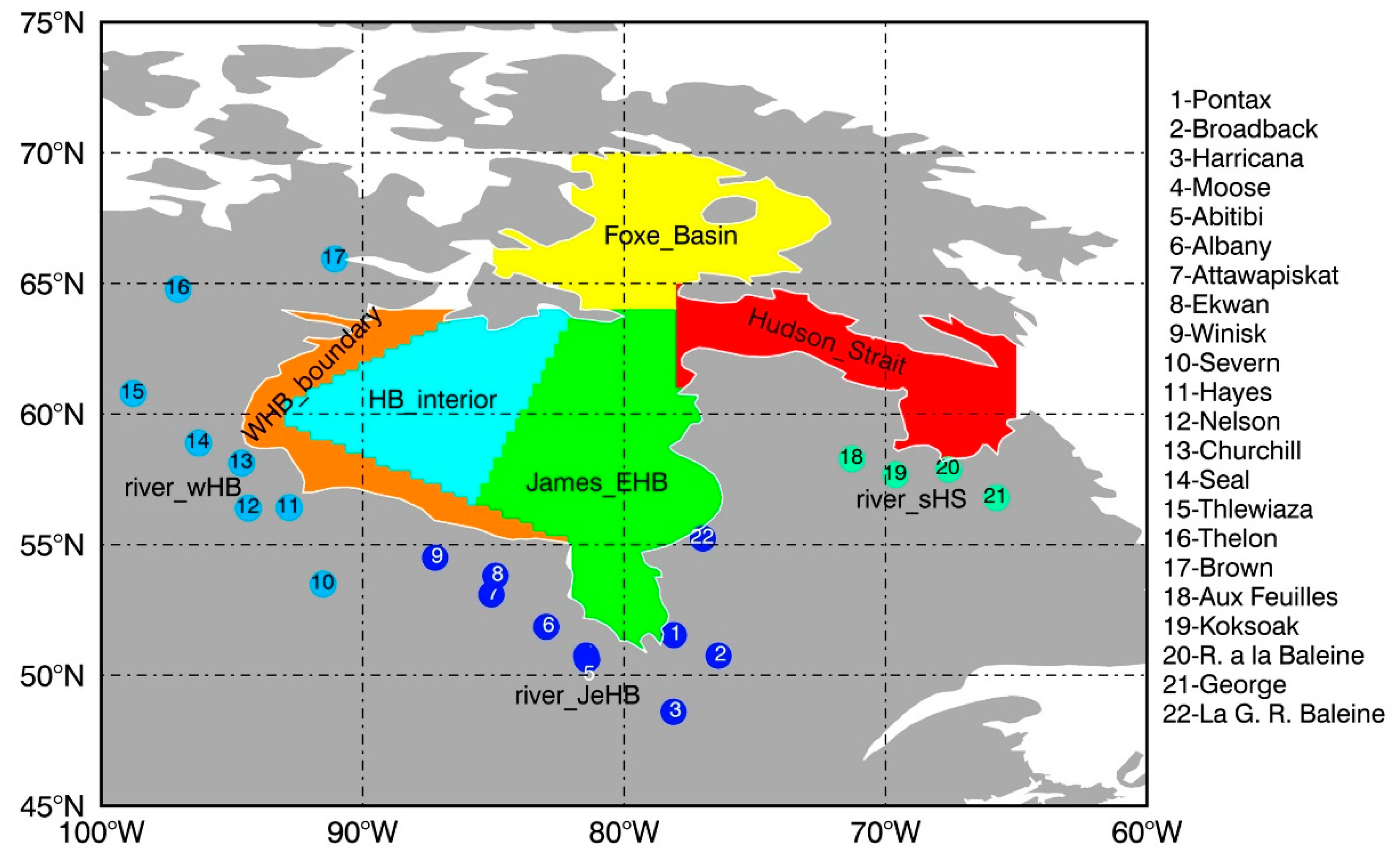
We analyze the spatial and temporal variability of satellite-measured salinity in the context of seasonal and interannual variability of each freshwater component of the local freshwater cycle (right hand side of Equation (1)). The study area is schematically shown in
Figure 1. We focus on the Hudson Bay proper, which is divided into three sub-regions according to the river water path and HB circulation pattern [
10]: the James and eastern Hudson Bay (James_EHB, green color), which is along the path of discharge from southern rivers; the Hudson Bay interior (HB_interior, cyan color) which has negligible direct input from rivers; the Western HB boundary (WHB_boundary, orange color) which is under the influence of river discharges west of HB. Freshwater contents will be analyzed in each sub-region or in HB proper with three sub-regions combined. SSS in the Foxe Basin (yellow color) and the Hudson Strait (red color) will also be examined as a reference. Data source and estimation method of each freshwater component including R, P-E, I
local, and H
adv are given in
Section 3.
4. Results
4.1. Satellite SSS in Hudson Bay
4.1.1. Seasonal and Inter-annual Variability
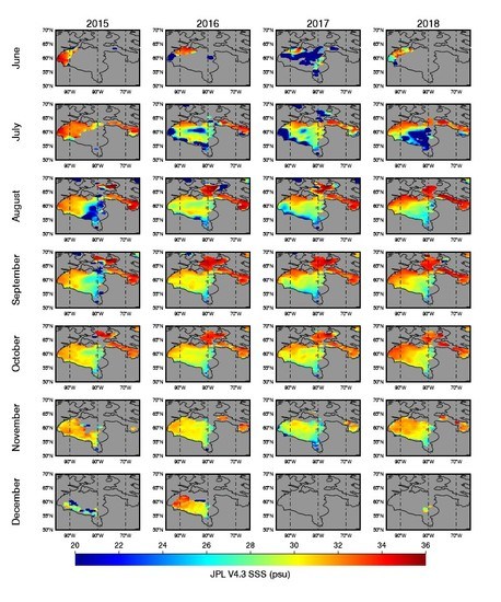
Figure 2 illustrates SSS
SMAP_JPL of June to December from 2015 to 2018 in the Hudson Bay System. This is the period when seasonal snow/ice melting creates open water areas in the bay, where remote sensed SSS is feasible. From January to May, the bay surface is mostly frozen. We see from
Figure 2 three phases in the seasonal evolvement of SSS: phase-1 ice melt (June and July), phase-2 open water (August-October), and phase-3 ice formation (November and December).
In phase-1, areas with available SSSSMAP_JPL retrieval first appeared in the northwestern HB in June, except in June 2017 when the onset of ice melt occurred much earlier than other years. That year, the entire northern part of the bay is covered by fresh water by June, which is consistent with the SIC data (not shown). The open water area spread southeastward in July covering most HB areas, with the only exception in July 2015 when most area in the eastern Hudson Bay still closed from south to north. For the July of the other three years (2016–2018), HB areas were all open, but the patterns of SSSSMAP_JPL are very different. In July 2016 and 2017 the freshening signature is observed along the western boundary, while in July 2018 a large area of freshening appears in the eastern HB.
In phase-2, when HB is completely covered by open water, the sea ice impact on the variation of SSS become minimal (as expected). In those cases, SSSSMAP_JPL shows a rather homogeneous spatial pattern: fresher in the southern HB, saltier in the northern HB, in the Hudson Strait and in the Foxe Basin. This pattern is consistent for the four years of study with very little interannual variance. This is also consistent with the fact that northern HB is along the path of advection from Hudson Strait, carrying salty seawater from the northern Atlantic Ocean; while southern HB is under the influence of river discharge. On the other hand, because of the Foxe Basin is dominated by sea ice, it is unclear whether the increase of salinity in Foxe Basin is the result of the Atlantic water intrusion or is due to sea ice contamination. Most interesting is the abnormal pattern observed in August 2015. A large fresh patch is observed in area mainly collocated with the late sea ice melt in July 2015. It is also interesting to note that the fresh signature along the HB western boundary observed in July 2016 and 2017 sustained in this open water phase.
In phase-3, the last two months of the open water season (November and December), available SSSSMAP_JPL observations diminish from north to south, accordingly with the progress of sea ice formation. We note the exception of December 2016 when the SSSSMAP_JPL was still retrieved in the large part of HB interior. This occurred because in December 2016 the freezing was observed later.
4.1.2. Difference between Satellite SSS Products
Here we briefly summarize the features observed in other remote sensed SSS products (
Figures S1–S3) in the Hudson Bay during the three phases and their consistency or inconsistency with respect to SSS
SMAP_JPL described above.
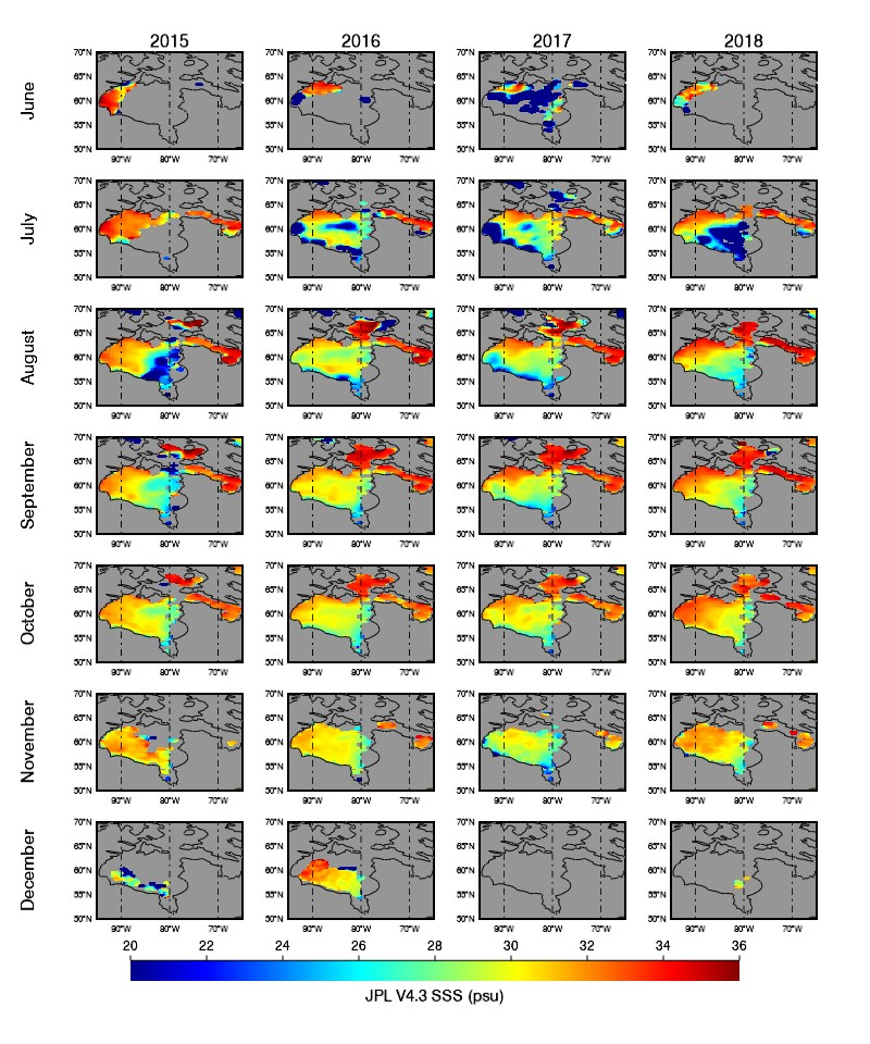
The
SSSSMAP_RSS (
Figure S1) shows similar features in all three phases as SSS
SMAP_JPL, particularly the major interannual anomalies, for example, the freshening pattern in area_James_EHB in August 2015; the late ice formation in area_HB_interior in December 2016; the early ice melting onset in June 2017; and the freshening in the majority parts of area_HB_interior and area_James_EHB in July 2018. The main difference between the two is that SSS
SMAP_JPL is much more permissive in the SSS retrieval near ice edge (SIC threshold of 3% vs. 0.1%), hence SSS
SMAP_RSS showed minimal retrieval during ice melt onset (June); incomplete coverage in area_HB_interior and area_James_EHB in July 2018; almost no retrieval in the Hudson Strait, the Foxe Basin, and near the coast for the entire season. Moreover, the fact that SSS
SMAP_RSS missed the freshening feature along the western boundary current not only in July 2016 and 2017 but also in the following open water phase, suggests possible differences in the land correction algorithm (which removes the land contribution to the brightness temperature measured in satellite footprint near coast) between the two SMAP SSS products.
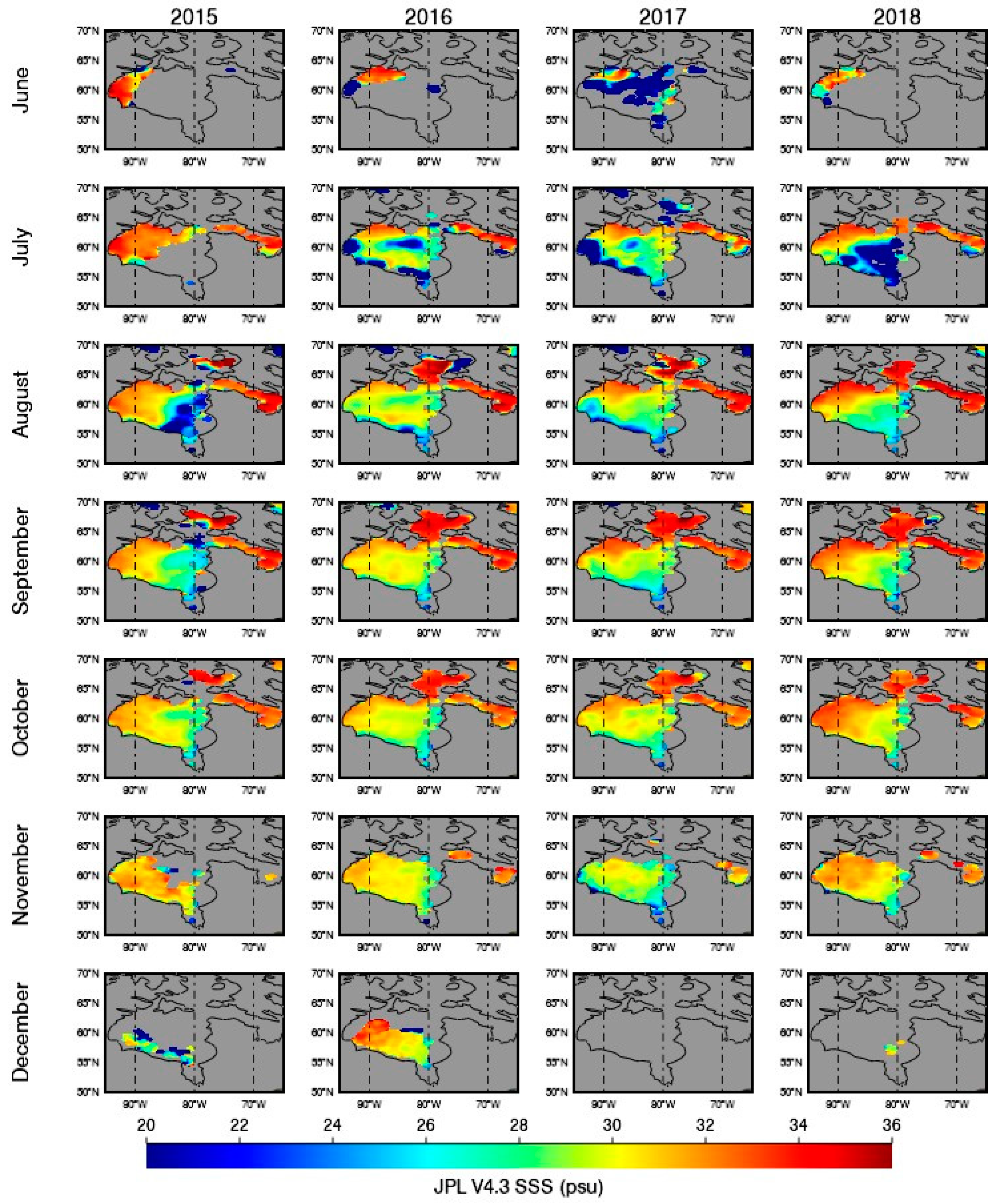
SSSSMOS_BEC (
Figure S2) in Hudson Bay is smoother in comparison with SSS
SMAP_JPL. Similar as SSS
SMAP_JPL, SSS
SMOS_BEC showed the ice melt onset started in the northwestern HB in June, the late melt in July 2015 and the early melt in June 2017 in HB interiors, the late ice formation in December2016, and the general spatial gradient of freshening from north to south. However, SSS
SMOS_BEC differs from SSS
SMAP_JPL mostly in the open water period (phase-2), such as in HB interior, although SSS
SMOS_BEC shows the abnormal late melt in July 2015, the pattern of SSS
SMOS_BEC in August is very similar as August of other years, i.e., show no impact of the sea ice late melt. This is probably because of the correlation radii used in the generation of the SSSSMOS_BEC product (321 km, 267 km and 175 km). They cause an excessive smoothing in this basin which limit the study of the freshwater dynamics in HB.
SSSSMOS_LOCEAN (
Figure S3) was much saltier relative to other SSS products. However, besides the bias, we can recognize in SSS
SMOS_LOCEAN the anomalous features observed by the two SMAP products (as described above), particularly for the fresh pattern in area_JeHB observed in August 2015, SSS
SMOS_LOCEAN has similar west-east spatial gradient as shown by SMAP products. However, along the western boundary of HB, SSS
SMOS_LOCEAN shows salty signature in contrast to the fresh signature observed in SSS
SMAP_JPL, and SSS
SMOS_BEC (SSS
SMAP_RSS has no retrieval in the area).
Since there are very few in situ salinity measurements in the Hudson Bay available to validate satellite products, below we will examine the SSS variance in the context of the inter-annual variability of freshwater inputs from river discharges, sea ice changes, and surface freshwater forcing (precipitation and evaporation). We identified that the anomalous fresh signatures described above mostly can be associated with anomalous regional freshwater inputs from different processes.
4.2. SSS Response to River Discharge
Significant discharge from individual rivers (
Figure 1) around the Hudson Bay starts in a narrow time window in late April to early May, except the Nelson River in west of the Hudson Bay, with year-round flow around 4000 m
3/s.
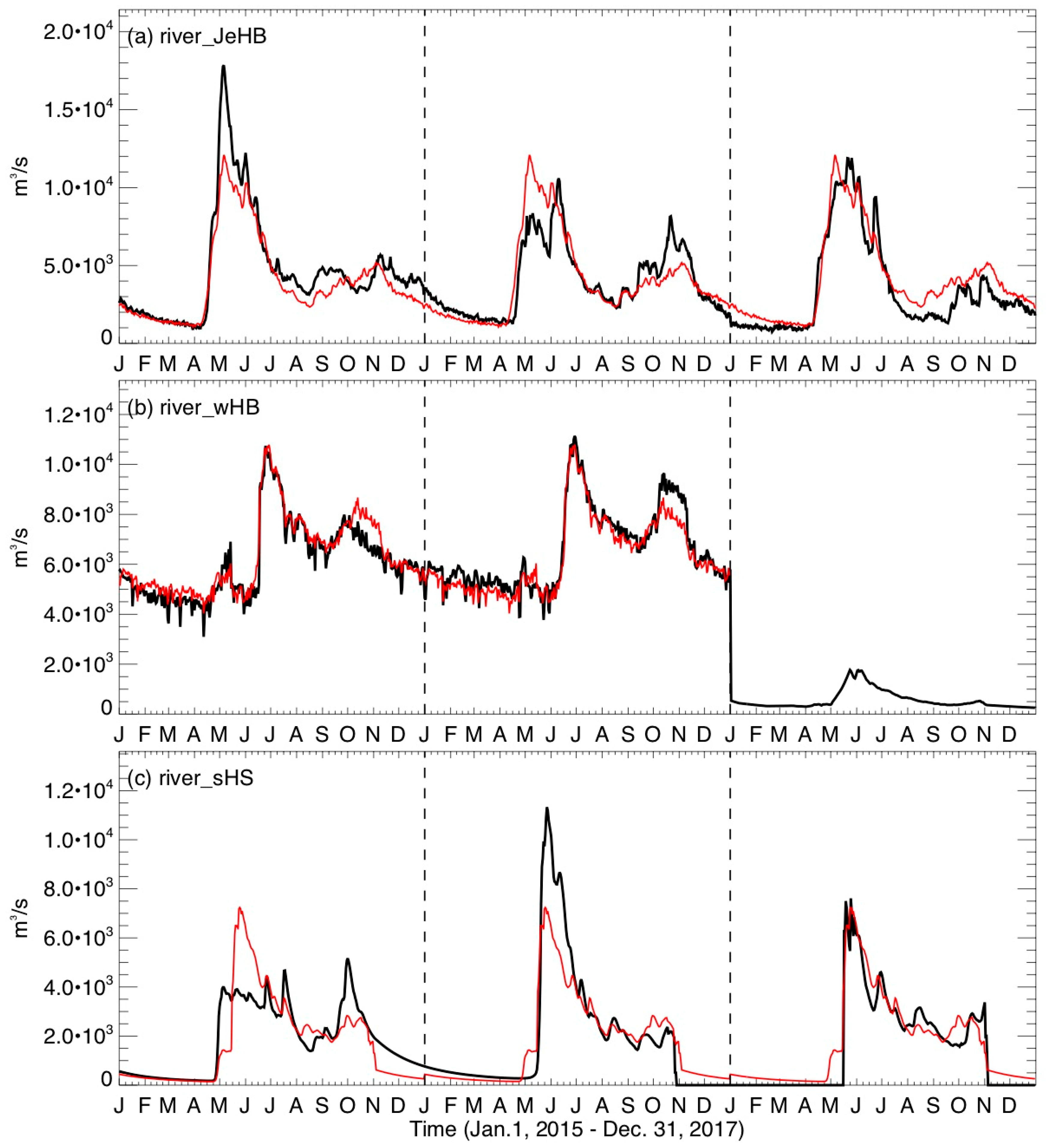
Figure 3 shows the daily discharge of each river group (defined in
Section 3.2) into the Hudson Bay from January 1, 2015 to December 31, 2017. Most river groups show two flow peaks: the first in May due to snow melt over land, and the second peak, smaller in magnitude, in October to November, likely as the result from the precipitation over basin. There were large inter-annual variations in the magnitudes of discharge. Here, we examine the possible linkage between anomalies of discharge and SSS patterns, focusing on the two sub-areas in HB under strong influence of river discharge: area_JeHB and area_wHB.
The James and Eastern Hudson Bay (area_James_EHB) is under the influence of the river group river_JeHB (Fig.3a). The freshwater from this group enters the southern area of the James Bay and joins the HB anti-clockwise circulation, which flows northward in eastern Hudson Bay. The first discharge peak in 2015 from this group reaches 1.7 x10
4 m
3/s, which is 50% larger than the three years average of 1.1 x10
4 m
3/s (
Figure 3a). The anomalous fresh signature observed by satellite SSS in August 2015 (
Figure 2) is right along the path of freshwater transport from river_JeHB. The total integrated flow from April to August is about 80.4 km
3 in 2015, which is 13.6 km
3 (or 20%) more than the three years average. We note that river_JeHB discharge peaked in May 2015, three months ahead of the low SSS observed by SMAP and SMOS in August 2015. Our hypothesis is that river discharge entered the bay through small opening along the coast and built up freshwater content underneath the ice pack. The river plume was then observed later by satellite when sea ice melt. We also note the discharge from La Grand River Baleine on the eastern coast of the Hudson Bay has a magnitude one order smaller than the James Bay rivers, suggesting the discharge anomaly of river_JeHB is mostly caused by the southern rivers. Another interesting feature of river_JeHB discharge is the moderate positive anomaly observed in October to November 2016 (second peak). Recall that all four SSS products provide valid salinity measurements in majority of Hudson Bay interior in December2016 (
Figure 2), in contrast to an almost frozen bay in December of other three years. It will be interesting to see/examine any linkage between the delayed freezing and the extra (relatively warm) water in fall from the southern rivers.
The Western Hudson Bay (area_wHB) is dominated by the boundary current from north to south of the anti-clockwise circulation around HB.
Figure 3b illustrates the discharge rate from river_wHB. Only two years of data are plotted since we have data available for most rivers in the groups up to the end of 2016. The contrast between these two years reveals a slightly positive (~2%) discharge anomaly in early 2016 (January to May) and a large positive discharge anomaly (~10%) in the fall of 2016 (October to November). Intuitively, one may attempt to link the fresher signature along the HB west coast in July of 2016 observed by SSS
SMAP_JPL with the positive river discharge anomaly, which injects freshwater to the bay and it is transported from north to south along the western boundary. However, the fresh signature in SSS
SMAP_JPL was three months earlier than the positive anomalous discharge from river_wHB. Although the SSS
SMAP_JPL shows the western boundary still fresher than HB interior from August to October 2016, the impact of river discharge cannot be established considering the reversal in events time. Using a 3-D sea ice-ocean coupled model with realistic forcing including river discharge, [
10] found the average transit time about three years, from river water input in near shore region to HB interior before outflow toward the Labrador shelf. Based on that, we speculate one possible source of the western boundary fresh signature maybe the result of the extra freshwater from the James and eastern Hudson Bay in 2015 open water season.
4.3. SSS Response to Surface Forcing (P-E)
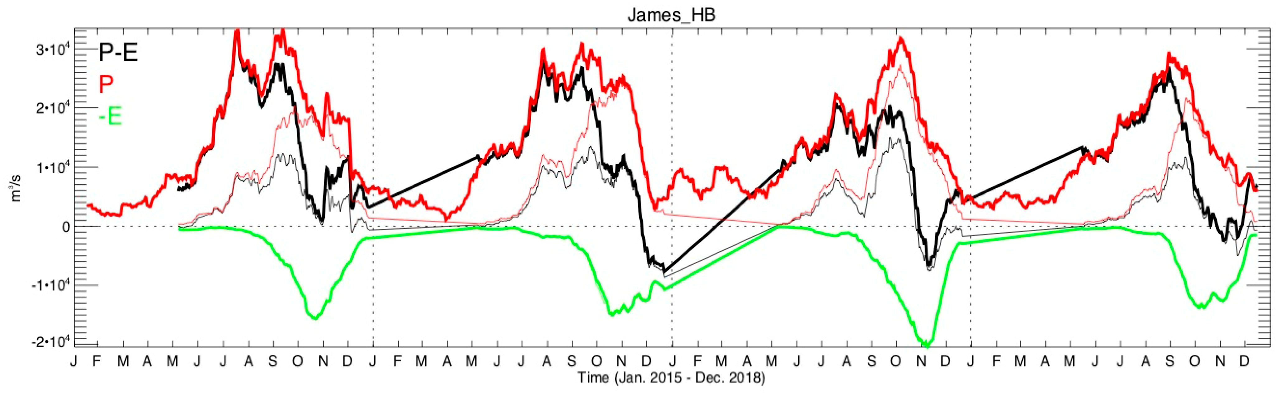
Here, we examine SSS response to the surface freshwater flux (P-E) in the Hudson Bay system. At the latitudes of the Hudson Bay, both P and E are small and opposite in phase for the period from June to December. E is higher than P for June to September with a transition from raining season (P>E) to evaporation dominated season (E>P) in September. Positive E represents freshwater from ocean to atmosphere through evaporation, and vice versa for negative E. In the wet season (June to September), GPCP P maps (not shown) indicate a maximum P ~ 5mm/day, with majority precipitation in south of 60°N over the southern HB and vicinity land area, and with large variations in the locations of maximum P. E is very small during the raining season (less than ~1 mm/day) and increases from September to December, reaching a maximum ~4 mm/day (not shown). Unlike P of GPCP, the OAflux E is only available for open water and affected by sea ice where E is masked as missing.
The net surface freshwater flux (P-E) is illustrated in
Figure 4. Clearly the role of surface freshwater forcing reverses in September. Before September, from June to August, P-E is positive across the Hudson Bay (dominated by rain); while after September, E exceeds P resulting negative P-E. The most interesting feature is the anomalous positive P-E across HB in July 2015, which overlaps with the area of anomalous low SSS (
Figure 2) one month later (Aug. 2015). This suggests while abnormal high discharge from river_JeHB building up the freshwater content underneath ice (
Figure 3), P-E also brought in more freshwater from atmosphere, contributing to the very fresh signature observed by satellites once ice melt (August 2015). On the other hand, P-E seems has no contribution to the abnormal fresh signature observed in northern HB in June–July of 2016 and 2017.
Figure 5 illustrates the time series of P, -E, and P-E integrated over the entire Hudson Bay (area_wHB + area_JeHB + area_intHB in
Figure 1), where two sets of time series of P and P-E are shown. The first set of time series (thick lines in
Figure 6) is P (and P-E) integrated over areas where P and E are available independently, refereed as P
1 and (P-E)
1. The second set (thin lines in
Figure 5) is P (and P-E) integrated over areas where both P and E is valid (a smaller area due to missing values in E), referred as P
2 and (P-E)
2. Note E is the same in (P-E)
1 and (P-E)
2 (the green line in
Figure 5). Basically, (P-E)
1 represents net surface freshwater inputs into HB no matter it is covered by ice or not; while (P-E)
2 represents net freshwater inputs into HB when its surface is open water. While the latter is more similar to the environment condition required for SSS retrieval, the former is a more accurate assessment for the seasonal accumulated freshwater content.
4.4. SSS and Freshwater from Sea Ice Changes
We estimate the freshwater flux from local sea ice changes I
local (Equation (2)). We consider only “critical location” where the matchup sea ice concentration C(x,y,t) is less than a prescribed threshold C
cut (e.g., 3%) in at least one of the two adjacent days involved in the temporal derivative using daily SIC data. Assuming a uniform ice thickness of 1 m as described in
Section 3.3., Equation (2) can be simplified as,
We argue that if both C(x,y,t) and C(x,y,t-Δt) are larger than the threshold (e.g., 3%), no SSS retrieval will be possible during the period, therefore I
local will be irrelevant to this study. Only SSS retrieved at “critical location” would catch the effect of freshwater resulted from sea ice changes. In cases of sea ice melting, we will have C(x,y,t) < Ccut while C(x,y, t-Δt) > Ccut and vice versa in cases of sea ice formation, C(x,y,t) > Ccut while C(x,y, t-Δt) < Ccut. Due to the fact that sea ice melt/formation in a specific location happens quickly, it is necessary to use SIC data with the highest temporal resolution as possible, i.e., daily SIC data (Δt = 1 day). We refer I
local obtained with C
cut = 3% as I
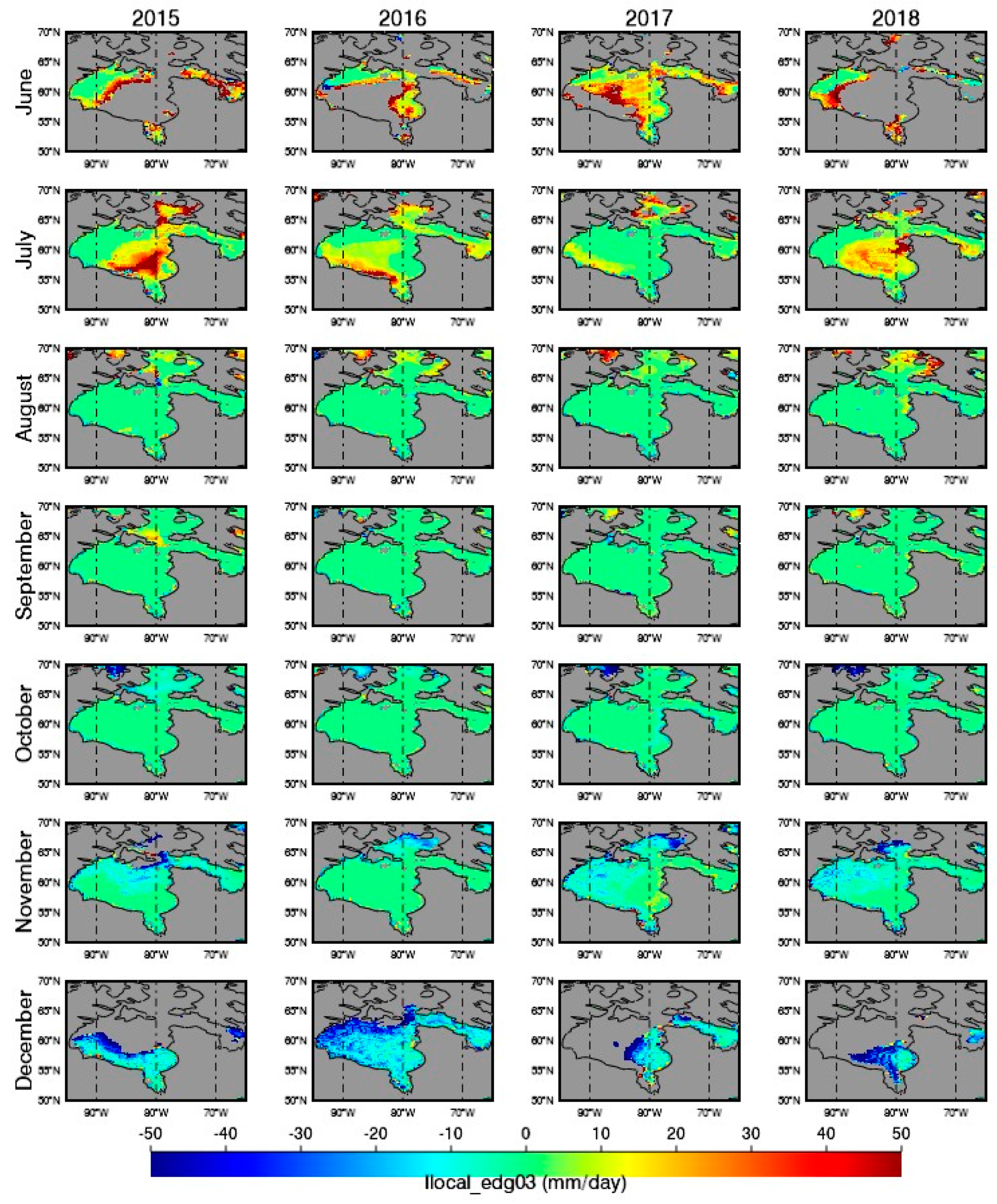
local3. Figure 6 shows the monthly I
local3, which is the average of daily I
local3. We observe several interesting features in I
local3. In phase-1 (ice melt, June and July), we found large inter-annual anomaly in I
local3 consistently with SSS
SMAP_JPL described in
Section 3.1. For example, the patch of negative I
local3 in area_JeHB in July 2015; fresh signature along the west-southern boundary in July 2016; and in area_intHB in June 2017, all can find their imprints in the SSS
SMAP_JPL (
Figure 2). For phase-2 (open water, August to October), as expected, I
local3 is near zero across the bay. The spatial coverage of I
local3 is also consistent with SSS
SMAP_JPL, particularly the late ice formation in December 2016. However, we should point out the slight difference of SSS remote sensing in observing the ice melt and ice formation phases. The freshwater inputs due to ice melt seems immediately reflected in the SSS fields, while the freshwater losses due to ice formation could not be observed in the similar manner because ice formation prohibits subsequent SSS retrieval.
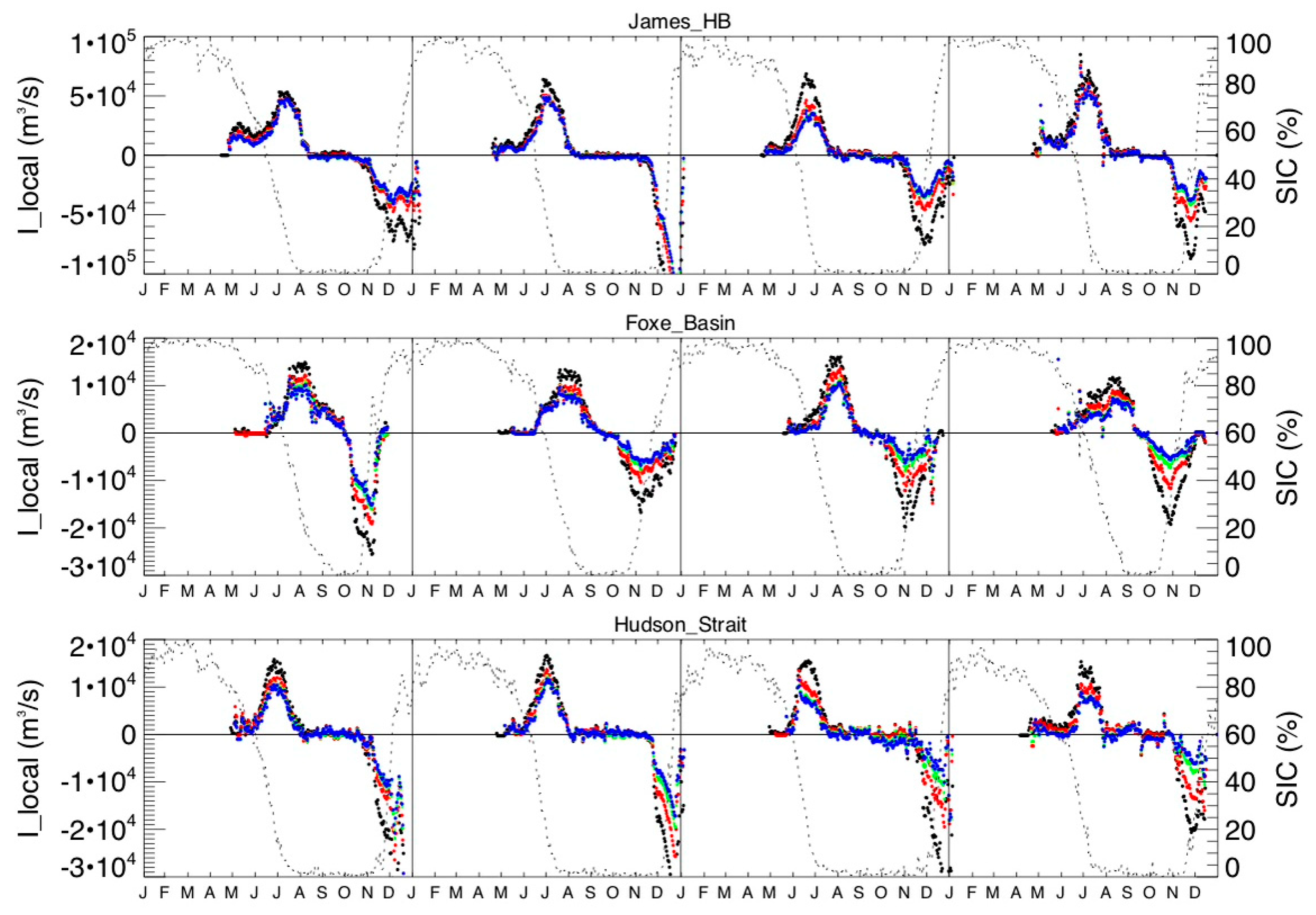
Figure 7 shows the daily time series of I
lcoal integrated in the sub-areas of the Hudson Bay system including the James and Hudson Bay, the Hudson Strait and the Foxe Basin. The I
local time series confirmed the yearly phase transition as described in the monthly maps. In the Foxe Basin, three phases reduced to two: ice melt phase transits to ice formation phase almost directly with a very short period in between. The total yearly freshwater inputs in the ice melt phase is the integration over time for positive I
local; and the total freshwater loses in ice formation phase is the integration over time for negative I
local. On the annual basis, area under positive I
lcoal roughly balance that under negative I
lcoal, resulting near zero net contribution.
As a reference, we repeated the calculation of Ilocal using different threshold for the “critical location”, for Ccut of 5%, 10%, and 20%, referred as Ilocal5, Ilocal10, and Ilocal20, respectively. We notice that temporal variation of Ilocal obtained using different Ccut are well correlated in terms of the timing of the ice melt/formation onset and transition between phases, as well as the time they reach positive/negative peaks. The magnitude of Ilocal increases with Ccut, but the spread between minimum and maximum Ccut varies. For example, δ3/20 (i.e., Ilocal20-Ilocal3) was very small in the melt phase of 2015 but reached 50% in the melt phase of 2017. Interestingly, the spread of ice formation phase (negative Ilocal) seems generally larger than that in the ice melt phase (positive Ilocal).
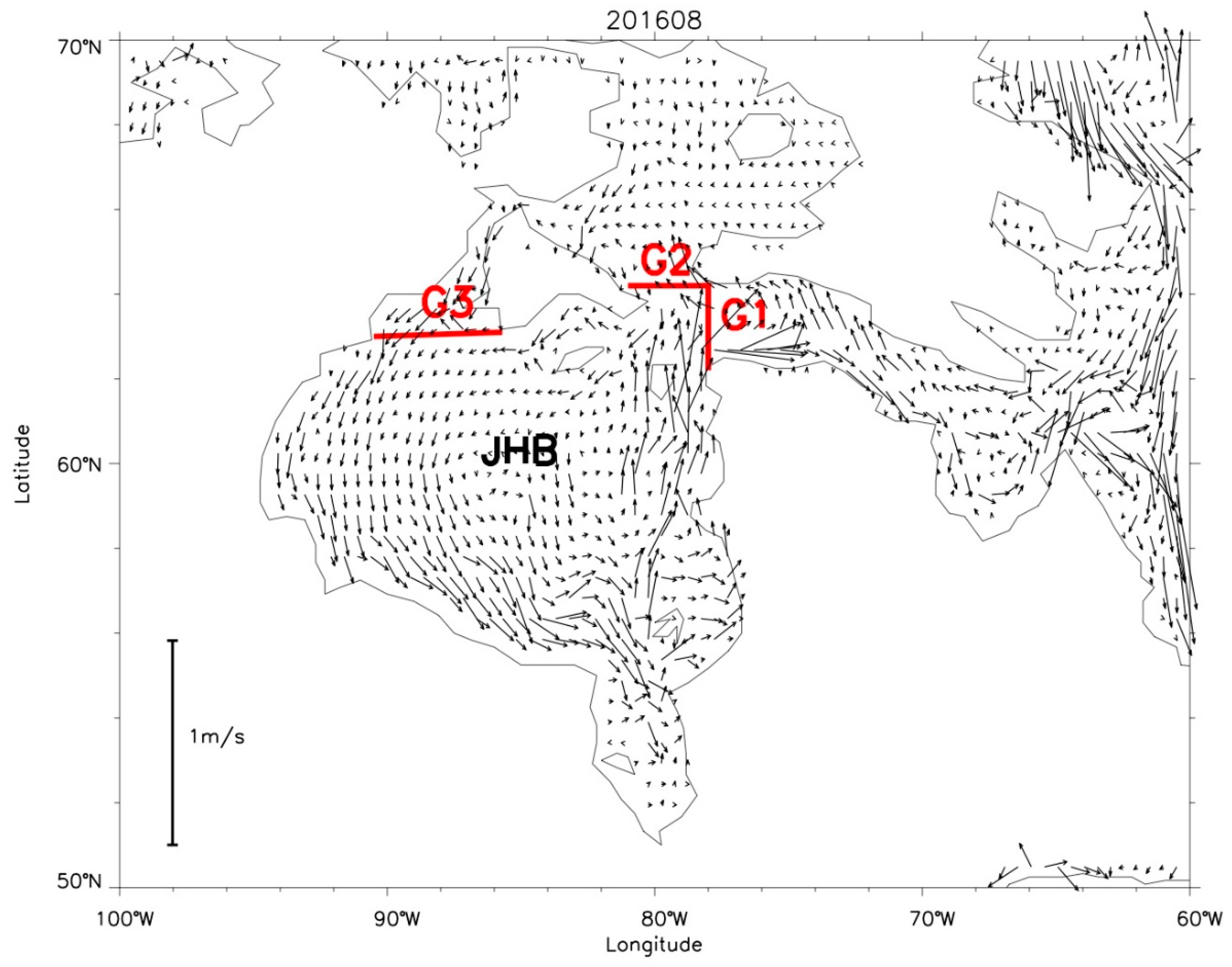
4.5. Salt Advection at Hudson Bay Gateways
The Hudson Bay is a self-enclosed system, connected with the world ocean circulation mainly through two main channels in the north (see red lines in
Figure 8). The channel at northeastern HB adjacent to the entry of the Hudson Strait east of the Southampton Island is schematically divided into two sections: one at the western end of the Hudson Strait (referred as G1), other at the southern end of the Foxe Basin (G2). The channel at northwestern HB located at the southern end of the Roes Welcome Saund between the Chester Field Inlet and the western coast of the Southampton Island, defined as G3. In
Figure 8, we show the HYCOM surface current of the Hudson Bay system in August, representing the summer circulation pattern. Following [
40], we calculate the total horizontal advective salt tendency through these gateways using the following formula:
where the D is the depth of surface layer (assumed 10 m),
is the surface current (vector), and S
g the sea surface salinity, both as function of location along the gateway and time, and
is a unit vector normal to the gateway section pointing into HB interior (grey arrows in
Figure 8) such that a positive value of
represents advection from outside into the Hudson Bay.
is a reference salinity value of the Bay as function of time which we obtained by averaging SSS over area of James_HB. Vol is the volume of the system, where the salinity tendency is under the influence of advected salt. The physical meaning of H
adv given in Equation (3), according to [
40], is that at a given time advective salt tendency equals to the difference of the salinity of advected water with respect to the salinity of water already in the system, uniformly diluted by the volume.
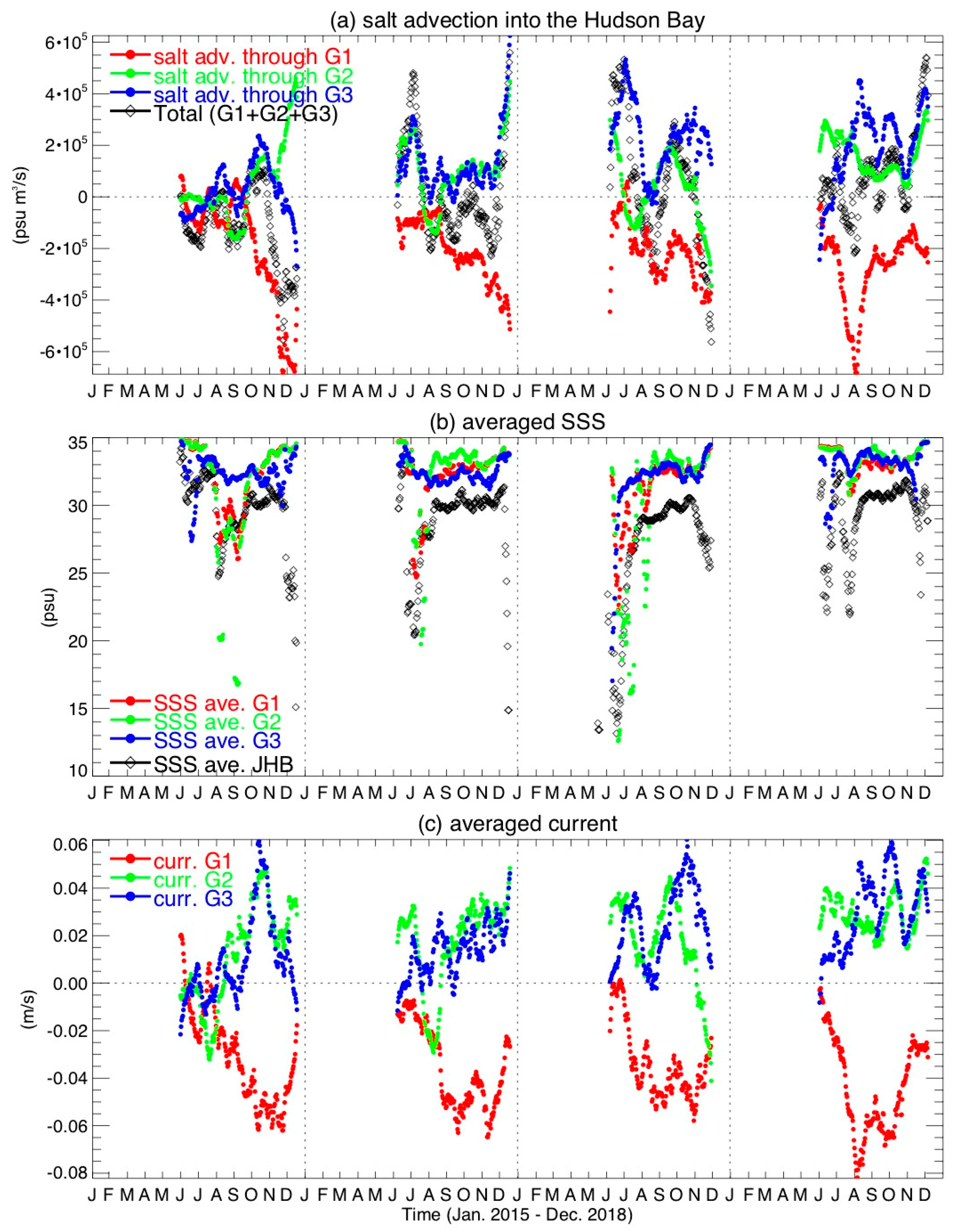
Figure 9a shows H
adv*Vol through HB gateways defined above, estimated by using daily HYCOM surface velocity and SSS
SMAP_JPL. Due to high sea ice coverage in the vicinity of gateways, the time series is noisy, hence a 30-day moving average is applied to data collected in ice melt season of each year. We see large interannual variance, but generally speaking, advection through G1 generates negative salinity tendency in HB, while advection through G2 and G3 produces positive salinity tendency in HB. This can be understood from the time series of SSS
SMAP_JPL (
Figure 9b) and HYCOM surface currents (
Figure 9c) averaged over each section. Throughout the ice melt season, SSS
SMAP_JPL (
Figure 9b) averaged over the Hudson Bay (including the James Bay) is lower than SSS
SMAP_JPL over all three gateway sections by more than 5 psu. The ocean current (
Figure 9c) averaged at G2 and G3 are from the Foxe Basin into the Hudson Bay, which brought in saltier water therefore has a tendency to increase the salinity in HB. On the other hand, currents at G1 is from HB to the Hudson Strait. Because SSS
SMAP_JPL at G1 is higher than SSS
SMAP_JPL within the bay, the transport at G1 basically advects salt out of the bay, therefore, the HB salt tendency caused by G1 transport is negative.
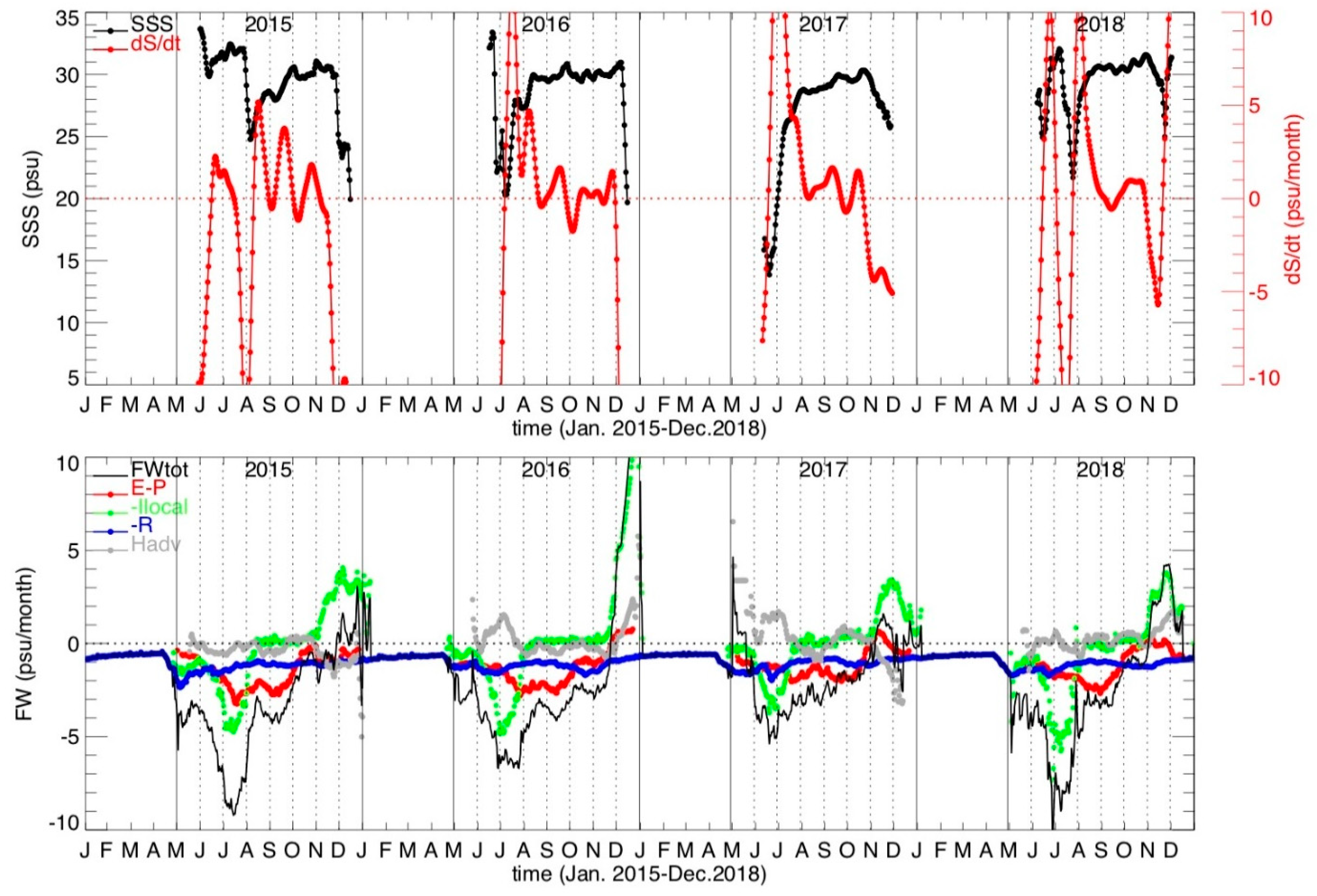
4.6. HB Upper-layer Salinity Budget
Figure 10 shows the daily time series of the salinity and salinity tendency (dS/dT) and each term of the salinity budget in the combined area of the James Bay and the Hudson Bay (indicated as JHB in
Figure 8), assuming h of 1 m. Daily SSS is obtained by averaging all available SSS
SMAP_JPL in JHB over open water, which is then used to calculate ∂S/∂t. S
0 in Equation (1) is chosen to be 31 psu here (approximately the HB annual average salinity). All freshwater contributions (RHS of Equation (1)) from different processes are converted into a quantity (i.e., the water depth result from freshwater input uniformly spread over the area under consideration) so they can be directly compared. For I
local and P-E, we perform area integration over the selected domain and averaged by the domain area to obtain their vertical freshwater inputs to the surface layer. In that sense, freshwater removed during ice growth (negative I
local) are treated as evaporation, and the freshwater added by ice melt (positive I
local) are treated as precipitation [
16]. Freshwater from river discharge and advection through HB gateways are converted to a surface flux term by spreading it uniformly over the surface area of JHB.
The seasonal evolvement of salinity (
Figure 10, top) is generally consistent with the three phases described in
Section 4.1, i.e., ice melt, open water, and ice formation (see
Figure 2). Clearly the freshwater contribution was dominated by ice melt in phase-1, reaching its maximum late June to early July, and trending earlier during the four years examined. It is interesting to note that after reaching its lowest early in the season, SSS quickly recovered to about 30 to 31 psu. During this recovering period, the salinity tendency from freshwater inputs (
Figure 10, bottom) remained negative, suggesting other process may play a role in diluting the surface freshwater produced by ice melt. In phase-2, SSS fluctuates at a small range and slowly increases, dominated by the influence of P-E and river discharge although later should be taken with pepper and salt due to lack of data for some major rivers after 2017. The salinity budget in phase-3 seems puzzling. While the salinity tendency from freshwater (RHS of Equation (1)) is positive mainly from ice formation as expected, SSS show sharp drop with negative ∂S/∂t for the last two months, except December 2018. This is because the ice formation in the Hudson Bay started from north, which left SSS retrievable area in the south where SSS is generally lower than northern area. Salt advection through northern channels is small comparing with freshwater contribution from other processes.
5. Discussion
How to select an appropriate SIC threshold for SSS retrieval is tricky. On one hand, it is unknown how high the sea ice percentage in a footprint is correctable without severely interferences with the true SSS signature. On the other hand, if SSS is only retrieved until sea ice completely melted, it may miss the most critical moment to monitor the salinity response to the sea ice contribution in understanding the regional freshwater variability. Some of the differences observed between SSS products are beyond the ice mask or threshold difference. For example, SSSSMAP_JPL retrieves SSS where sea ice concentration (SIC) is less than 3%, while SSSSMAP_RSS requires a much lower SIC threshold, and SMOS is based on a totally different platform and retrieval process. Currently, an enhanced version of the Arctic SMOS SSS product is under development through the specific ESA project Arctic+ Salinity at BEC. This new SMOS product is focused on capturing small-scale ocean dynamics. So the interpolation scheme has been modified providing an effective resolution of 25 km. Understanding the differences between SSS satellite products based on a credible validation is urgently needed and extremely important not only to avoid false retrieval (e.g., due to undetected ice contamination) and also to future improvement of the retrieval algorithms of satellite SSS observations in polar regions.
In regard to surface freshwater forcing, we should keep in mind that both P and E at high latitudes are subject to large uncertainties. There are large biases in gauge observations for snowfall in the northern regions [
41]. The underlying mechanisms of some of those uncertainties are still unknown. One example is the negative E values over the Hudson Bay from June to August (
Figure 5). Although small in magnitude, its significance cannot be ignored because it suggests that the moisture transfer through evaporation at the air-sea interfaces in the Hudson Bay is from atmosphere to ocean, therefore adding to the freshwater flux from P. This is opposite to what we know in the tropical ocean.
6. Conclusions
This study examines the potential of SSS retrieved from currently operational L-band missions: NASA’s SMAP and ESA’s SMOS, in monitoring the surface freshwater in the Hudson Bay. We found that SSS reflects and links the upper layer freshwater contents associated with sea ice change, river discharge, precipitation, evaporation, and advection through the northern channels connecting HB with the Foxe Basin and the Hudson Strait. Early in the summer (June–July), the spatial and temporal patterns of SSS is dominated by sea ice melting with large scale freshening in a short time (weekly), which dissipates quickly (likely caused by vertical advection). During the period HB surface covered by open water (August –October), SSS is homogenous cross the bay and slightly increases consistent with the surface freshwater forcing, with decreasing P and increasing E, while large inter-annual anomaly is attributed to discharge input from southern rivers. During ice formation (November–December) SSS is expected to increase due to salt release during freezing. This is not well observed by remote sensed SSS, suggesting released salt may be advected vertically downward. The upper-layer salinity tendency based on budget analysis suggests the dominant role of sea ice melt, followed by surface forcing and river discharge. The salinity tendency caused by salt advection from northern channels is small comparing with other processes.
We emphasize the explorative nature of this study, from two perspectives. On one hand, we are fully aware that current satellite SSS products in polar regions have large uncertainty and limitations, which may or may not be overcome based on current L-band measurements. In cold water, L-band sensitivity to seawater salinity largely degrades (this depends in future mission). Moreover, the accuracy of dielectric constant model at very low temperature is questionable. Further, lack of sea ice correction in the SSS retrieval algorithm, i.e., un-accounted contribution of sea ice emission in the scene mixed with ice and water, also causes error in retrieved SSS (this is on-going work).
On the other hand, results presented here encourages application of satellite SSS in various research across the polar regions. It suggests that satellite SSS from current L-band measurements may potentially be useful, not only in the Hudson Bay but also in the Arctic Ocean. With its semi-annual sea ice coverage, the Hudson Bay represents a scenario of the Arctic Ocean, where rapid changes related with climate warming are urgently calling for satellite monitoring. While the international remote sensing community gathering momentum for future missions better designed for polar observations, there are urgent needs to analyze currently available, more than one decade of SSS data since the launch of SMOS. Studies of satellite SSS can also help to identify problems in the satellite retrieval algorithm. Future improvement of satellite capability in monitoring the polar region can particularly benefit from, for example, extensive in situ salinity measurements near ice edge at onset of ice melt and formation and process studies using models with satellite data assimilation.

 ,
, 


