The Least Square Adjustment for Estimating the Tropical Peat Depth Using LiDAR Data


Department of Geodetic Engineering, Faculty of Engineering, Universitas Gadjah Mada, Jalan Grafika No. 2, Yogyakarta 55284, Indonesia
*
Author to whom correspondence should be addressed.
Remote Sens. 2020, 12(5), 875; https://0-doi-org.brum.beds.ac.uk/10.3390/rs12050875
Submission received: 31 December 2019
/
Revised: 4 March 2020
/
Accepted: 5 March 2020
/
Published: 9 March 2020
(This article belongs to the Special Issue Remote Sensing of Peatlands II)
Abstract
:High-accuracy peat maps are essential for peatland restoration management, but costly, labor-intensive, and require an extensive amount of peat drilling data. This study offers a new method to create an accurate peat depth map while reducing field drilling data up to 75%. Ordinary least square (OLS) adjustments were used to estimate the elevation of the mineral soil surface based on the surrounding soil parameters. Orthophoto and Digital Terrain Models (DTMs) from LiDAR data of Tebing Tinggi Island, Riau, were used to determine morphology, topography, and spatial position parameters to define the DTM and its coefficients. Peat depth prediction models involving 100%, 50%, and 25% of the field points were developed using the OLS computations, and compared against the field survey data. Raster operations in a GIS were used in processing the DTM, to produce peat depth estimations. The results show that the soil map produced from OLS provided peat depth estimations with no significant difference from the field depth data at a mean absolute error of ±1 meter. The use of LiDAR data and the OLS method provides a cost-effective methodology for estimating peat depth and mapping for the purpose of supporting peat restoration.

1. Introduction
Peatland degradation threatened the sustainability of tropical peatland ecosystems. It is caused by simultaneous or sporadic events of deforestation [1], groundwater table decline [2,3], peatland drought [4] and subsequent wildfires [1,5,6], carbon emissions, and peat subsidence [4,7,8]. This condition has occurred in almost all tropical peatlands, including those found in Indonesia [9,10]. To reduce the environment and economic impact from peat fires, Indonesia has to improve its peat wildfire prevention and implement peat restoration management [11]. Effective and efficient peat restoration, especially in degraded peatland areas, requires detailed topographic and peat depth data to plan operational restoration actions. Providing decision-makers with high-accuracy topographic and peat depth data for peatland restoration actions became more imperative after the extensive wildfires in 2015 and the subsequent enactment of Presidential Decree No. 1/2016 [12].
Peat depth can be obtained by measuring directly on the field, or by modeling based on surrounding characteristics that yield an estimate of peat depth. One method to determine peat depth is by field drilling. Although this method produces highly accurate data, it comes with high costs and labor time. Peat depth probe data is used as a determinant of the shape of bedrock basins within peatland areas [13,14]. Another method used to characterize bedrock is to use a geophysical (radiometric) method that include both airborne and ground-based geophysical systems. The newest example in the use of airborne systems is the application Airborne Electromagnetic (AEM) to quantify peat thickness of tropical peatlands [15]. Ground-based systems include the use of Gamma-Ray Spectrometer (GRS) and Ground Penetrating Radar (GPR) [16]. The use of GPR produced peat depth data that give an excellent correlation to the manual drilling method [17], which can reduce the survey time. However, the use of ground-based systems does not provide information about surface elevation [15]. This method does not disturb the peat ecosystem, but this measurement is considered expensive and time consuming [17]. To acquire elevation information, some researchers utilize Shuttle Radar Topography Mission (SRTM) data to derive the elevation of the ground. In order to derive the elevation of the ground surface, researchers have used curve-fitting applied to the SRTM elevation to get the shape of the ground surface [13]. Others use the results of land cover classification as an elevation reduction parameter from Digital Surface Model (DSM) to Digital Terrain Model (DTM) [18].
The modeling of soil characteristics has been developed and applied in soil mapping. Maps are created based on field survey results, which are then delineated, interpreted, and modeled by following the surrounding soil characteristics [19,20]. One of the soil characteristics is soil depth or peat depth. Some of the methods usually used in the prediction of soil properties have been previously reviewed and reported in the literature [20,21]. Several methods commonly applied for depth estimation are corpt, scorpan, trend surface, and kriging [20]. Other researchers also used univariate regression, multilinear regression, statistics, and linear regression methods [14,22]. Different techniques to estimate soil depth include multivariate geostatistics [16,22], inference modeling [23], and deep machine learning [18,24]. One of the methods that has not been used to estimate peat soil depth is the Ordinary Least Square (OLS) method.
The OLS method is a univariate geostatistics of linear modeling. This method can be applied in the prediction of soil classes [16] and soil properties. Each of the covariates in the prediction of peat depth can be identified based on their effects in the prediction equation by applying the following conditions: (1) mutually independent, (2) minimum in mean and error, and (3) normally distributed data [20]. Many researchers have used the OLS method in soil property modeling. However, the use of this method in estimating peat depth has never been applied directly. Modeling using this OLS method involves some parameters that can be used to obtain better prediction results.
As a peat depth estimation method that has been used by other researchers, some covariates are believed to affect peat depth estimation differently. These covariates are organism activities, topographic conditions, spatially relative positions [18,20], land cover, and geological aspects [25]. Topographic covariates consist of slope, aspect, curvature, flow accumulation, wetness index, stream power index, landform classification, vegetation index, and soil map [26,27,28]. Peatland visual conditions also have a specific correlation to the existing peat depth, i.e., length and slope condition, land cover, vegetation, and the groundwater surface [14,29,30].
The specific gravity value in peatland also has a close relation to moisture, peat decomposition, and mineral content factors. The higher the mineral content in peat soil, the larger the specific gravity value [31], the closer the peat surface is to the mineral soil and the larger the specific gravity value is in that location. Subsequently, the values of specific gravity can also be calculated to yield the gravity disturbance model [32,33], which represents peat depth in a particular area. Gravity disturbance (δց) is defined as the difference in value between the potential gravitational gradient (ց) and the normal gravitational potential gradient (γ) at the same location (h, λ, φ), as obtained using Equation (1) [32,34].
Each factor is a covariate used in peat depth modeling and may have a dominant effect, little effect, or even no effect at all. The influence of different covariates can be determined throughout parameter testing by statistical calculations. Therefore, identification of the impacts of the parameters must be analyzed. Thus, the uniqueness of the area and each parameter’s effect in this peat depth approach can be identified to obtain more accurate estimation results.
An accurate digital terrain model (DTM) is also needed to increase the accuracy of the estimate of peat depth. The DTM is necessary to derive topographic covariates and other spatial parameters. One common approach applied in peat depth estimation is the use of Global Digital Elevation Models (DEMs), including the use of the United States Geological Survey’s Digital Elevation Model (USGS DEM) [14] or The Shuttle Radar Topography Mission Digital Surface Model (SRTM DSM) [18,24,27]. These DEMs are usually derived into a DTM by reducing the elevation based on the type of land cover in order to obtain the bare earth surface. Land cover types can be obtained from the Landsat satellite images [24], Sentinel, and Advanced Land Observing Satellite of the Phased Array type L-band Synthetic Aperture Radar (ALOS PALSAR) [18]. Consequently, the application of a better quality DTM is required in order to achieve more accurate peat depth estimations. One of the alternatives is the use of Light Detection and Ranging technology known as LiDAR DTM.
Applying OLS methods in order to perform peat depth modeling by utilizing the above-mentioned covariates is feasible considering its applicability to classify vegetation and crop type using remote sensing methods [35] to estimate gravitational data. The geoid model [34] can be used to refine the estimation of the parameters in digital soil mapping [36], and to predict soil attributes and classify soil classes [20]. However to the author’s knowledge, the usability of this technique for peat depth estimation has not been tested elsewhere. This study estimates peat depth by the elevation of the mineral soil layer (substratum), based on the conditions of topography and spatial relationships. Testing the quality of the results obtained was conducted in order to evaluate the feasibility of this method for predicting the peat depth. We also evaluated the reduction of the amount of input data in the determination of the estimation equation in order to examine the efficiency of peat depth measurement in the field.
2. Materials and Methods
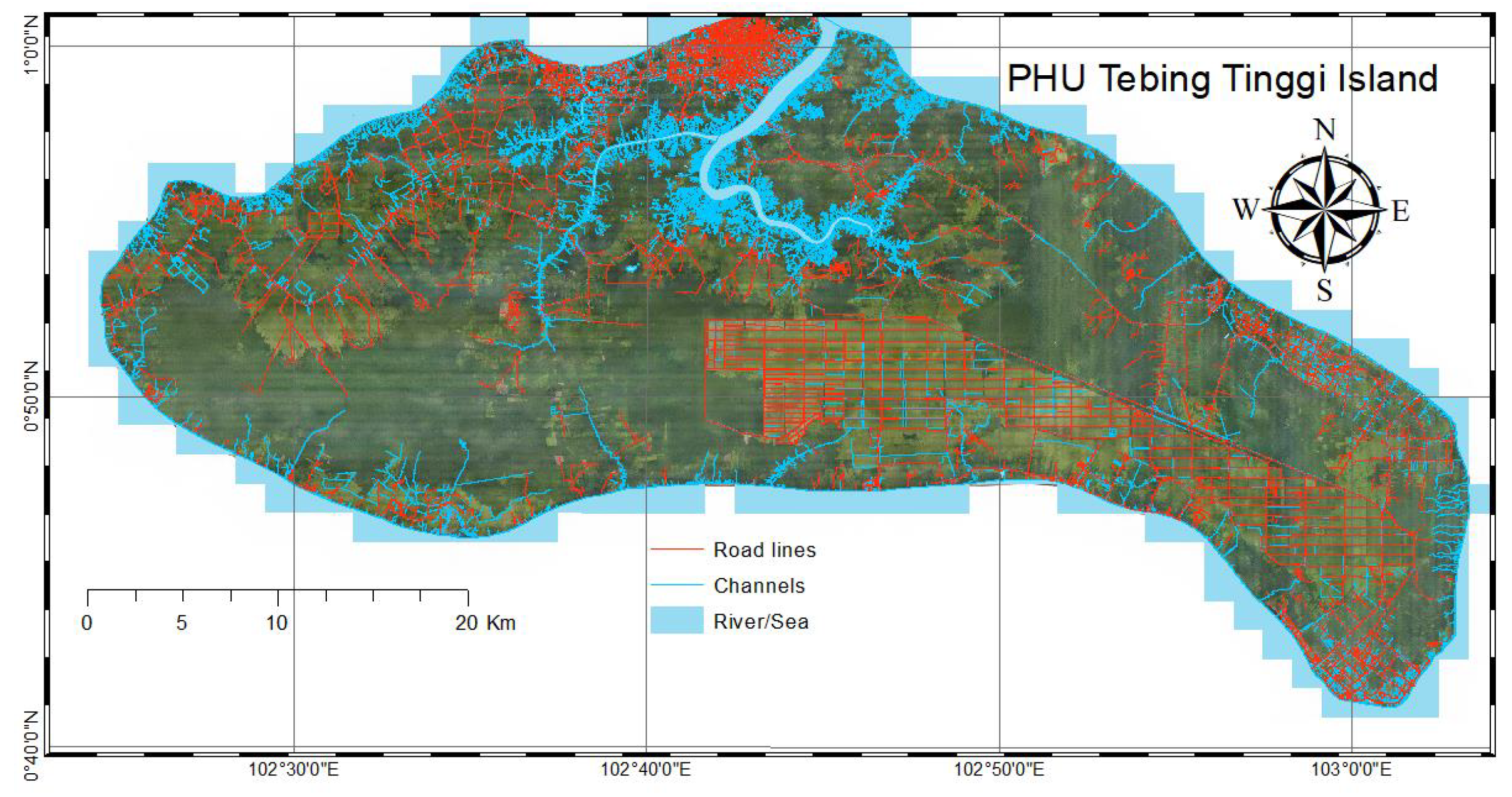
The study site was located in the Peat Hydrological Unit (PHU) of Tebing Tinggi Island, which is located in Meranti Regency, Riau, Indonesia. This PHU is one of the outer peat islands in Indonesia, which has a total area of 138,748.96 Hectares. The land cover of this PHU is dominated by plantation areas, primary forests and small portions of settlement and livestock farming areas. This peat island is topographically classified as a flat area, with a height difference from the shore to the peat dome of not more than 13 m. The PHU is divided into two peat domes. Village residents mostly live near the river and coastal areas. As clearly seen from aerial photos, irregular patterns of houses and village roads are located around waterways and river streams. Massive plantations and canal developments are located at the eastern side of the peat dome, where street and canal networks in blocks can easily be seen in Figure 1.
The data used for this research consist of: (1) Geological maps of the Siakinderapura, Tanjung Pinang, and Bengkalis areas with a scale of 1:250,000 from Geological Research and Development Center (P3GL) Republic of Indonesia; (2) Gravity disturbance data of the Tebing Tinggi Island area [37] calculated using the Satellite Gravity Gradiometry Ultra-high Gravity-field Model (SGG-UGM-1) gravity model derived from the Earth Gravitational Model 2008 (EGM2008) and the Gravity Field and Steady-State Ocean Circulation Explorer (GOCE) satellite data, (downloaded from http://icgem.gfz-potsdam.de/calcgrid); (3) Peat soil mapping data collected by The Ministry of Environment and Forestry, Republic of Indonesia, generated using ground-based peat probe survey data with a transect pattern for each 500 meters distance between drilling points and 1 km interval distances between the transects, (see Section 3.2. in more detail); (4) Aerial orthophoto with a spatial resolution of 10 cm, taken using a medium format metric camera [38]; and (5) a DTM generated from LiDAR measurement data from the Peat Restoration Agency (BRG), Republic of Indonesia [38]. Ground spatial distance of the DTM is 50 cm. The DTM is generated from filtered point clouds, which are free from the elevation of non-ground layers. Aerial orthophoto and DTM data were acquired by BRG in 2017.
2.1. The Covariates
The data were initially processed to gain covariates used as parameters in an equation for estimating the peat depth. These parameters are depressionless DTM, geological condition, slope position index, landform, valley depth, vertical distance to channels, topographic positional index, topographic wetness index, and distance to the nearest river. These parameters were acquired in the form of raster data from the above-mentioned materials.
Topographical conditions were modeled by doing preliminary editing of the DTM data in order to reduce the depression error, which can cause inaccuracy in water flow assessment using GIS. The principle of depression editing is based on the filling in of hollows on the ground surface [39,40]. The elevation reference plane of the DTM was determined using the global geopotential model (EGM2008), which was fitted to the local mean sea level derived from tidal observations. This fitting calculation was performed in order to obtain the best local vertical reference plane [41].
The resulting depressionless DTM was then used to determine the flow direction of the water on the ground surface. There are several principles used to determine the flow direction based on the DTM data. One of them is the D8 method. The basis of this method is to evaluate a single-pixel of DTM raster data by viewing eight surrounding pixels in the vicinity (3 x 3 window). By viewing the eight other elevation values, the water flows from the selected pixel to the pixel with the lowest value [42]. By following the direction of the subsequent water flow, the flow accumulation and the existing stream can then be determined [42].
After depressionless DTM and flow direction models were derived, other topography parameters were then identified and determined. Valley depth reflects vertical distance from the ground surface toward the canal/river network, which indicates local relief conditions. The valley depth is defined as the interpolation result of the difference in elevation between a certain point on the ground surface and the ridges. The height of the ridges is a vertical distance calculated with respect to the channel network. The vertical distance to channel network is an elevation difference between the ground surface and the surrounding base of the canal network [39].
Peat depth can also be observed based on the ground elevation of a specific location and the surroundings. The sub-stratum conditions under peat soil tend to be almost flat in a narrow area. Relative ground elevation difference to the surrounding area can be identified using the topographic position index. Elevation difference identification with this topographic position index is based on the ground elevation difference computation of a cell compared with the average ground elevation in the vicinity [43]. The surroundings elevation factor included a wider range of area, which gives an index value that reflects the common condition of the area. Based on this topographic positional index, slope and landform of the terrain can be classified as presented in Appendix B.
Peat depth has a relationship with the wetness condition, which in this study was represented by the wetness index. The wetness index values were determined by computing the surface flow accumulation [28,39,44]. In this study, the transmissivity value was assumed to be constant for the entire PHU area. Areas close to the river networks tend to have higher wetness index values [44]. Areas close to artificial channel networks located in the industrial plantation forest concessions have relatively lower wetness index values. The calculation for determining the topographic wetness index is presented in Appendix B.
Spatial proximity to the river/shoreline reflects the peat depth condition of the surrounding [18]. In general, the closer an area is to a river or shoreline, the thinner the peat depth is [45]. The positions of the rivers in the peatland area were identified after stream-order modeling was completed. The river with the highest stream-order is a large river or a main channel in the peatland. Spatial proximity of a point to the nearest river can be determined using Euclidean distance in GIS software [18,45,46].
2.2. Peat Depth Estimation
Equation modeling was conducted by including the ten parameters mentioned in Section 2.1. This modeling was performed using the parametric method of OLS. This method was used to determine a model of the peat depth estimation equation and the coefficient of each parameter. In this case, the equation applied a uniform weight (identity matrix), as shown in equations (2) to (4), [47,48].
where A is the coefficient matrix, X is the estimated parameter matrix, L is the result matrix, and V is the residual matrix.
Matrix A (Equation (3)) is a matrix of coefficients consisting of the values of each covariate determining peat depth. Matrix X is a parameter matrix. Its value shows the effect of each parameter in determining peat depth in this method. Matrix L is a result matrix, which was filled by the real peat depth data from the field survey. Matrix V is a residual matrix that indicates the accuracy of each covariate. Matrix X is a resulting value that can be determined by Equation (5) referring to the formula specified in [47,48], as a follow:
where X is the estimated parameter matrix, A is the coefficient matrix, P is the weight matrix, and L is the residual matrix.
Given that every point from the drilling results of the soil survey is a singular datum whose accuracy is unknown, the weight matrix (Matrix P) used in this equation is an identity matrix. However, if the input is a group of measurement data that has standard deviations and averages, then the Matrix P will be filled by the values of the standard deviation for each associated cell. In order to get better results, the calculation can be done iteratively, commonly called the "Observation Equation Model with Observed Parameters" [48]. It is an iterative procedure which uses the calculation results of the first process for the next computation. The equation used in this work is a parametric method of OLS, in which the observed parameters were used in determining the coefficient matrix.
The process of determining the peat depth estimation equation was performed in several steps, involving 100%, 50%, and 25% of the observed field data of peat depth. Data selection was conducted by a random sampling strategy. The use of different amounts of data was done to evaluate whether or not less data usage would give an insignificant difference comparing to the full data usage. As peat drilling activities are time consuming and costly, LiDAR data are a means to increase cost effectiveness and multi-purpose uses.
2.3. Raster Operation
Based on Equation (4), coefficients for estimating peat depth values were derived. The coefficients were then applied as multiplier factors in the raster operation using GIS software. Arithmetic operators were used in the raster operation involving all raster data representing ten parameters. The result of this raster operation yielded a raster data model, which showed a peat depth value in every pixel position. The resulting peat depth model was then combined with the depressionless DTM to identify the mineral soil position lying underneath the peat soil layer.
Three-dimensional visualization through longitudinal profile and cross-sectional views was applied to represent the surface profiles of peat soil and minerals. This profile view can also be used to visually inspect the distortion values between the surface model and the measurement data.
2.4. Statistical Testing
Testing procedures were performed to ensure that data used in the equation modeling were free from both outliers and systematic errors. Additionally, testing of parameters and obtained results were also conducted to calculate the parameter significance. By filtering out outliers held using a global test, the outliers evaluation was executed by following Baarda’s data snooping rules with Pope’s Tau testing, as is displayed in Equation (6) [48]. The testing was applied to each residue of the previous calculation results.
where the τα/2 is a critical value at the level of significance α and degree of freedom r, S0 is a posteriori estimated variant factor, qii is the variant residual value.
After identifying data that contained outliers, an estimation equation modeling was then performed without enclosing outliers. This process was used to determine the coefficient of each equation parameter. Parameter identification had a significant effect on the estimation equation, which was tested by using the Student t-test. This parameter significance test is shown in Equation (7) [47].
where t is a critical value at the level of significance α and degree of freedom r, xi is the estimated parameter, μo is the true value of the parameter, σii is the standard deviation of the estimated parameter, and n is the number of observation equations.
The usage of peat depth drilling data in estimation equation modeling considered 3 scenarios of different amounts of data, which involved 100%, 50%, and 25% of the field dataset. Then, the results of those estimation models were statistically tested. This study was performed to know whether or not less data usage could be used to generate statistically equal data. This testing was done by using the Student t-test, as displayed in Equation (7). Furthermore, the quality of estimation results was determined from the calculation of dataset accuracy into a Mean Absolute Error (MAE) value. The value of MAE was determined using Equation (8) [47].
where MAE is the mean absolute error, f(xi) is an estimated value based on the modeling result, xi is the true value of the field measurement, and n is the number of peat depth data.
3. Results
3.1. Peat Depth and Mineral Soil Elevation
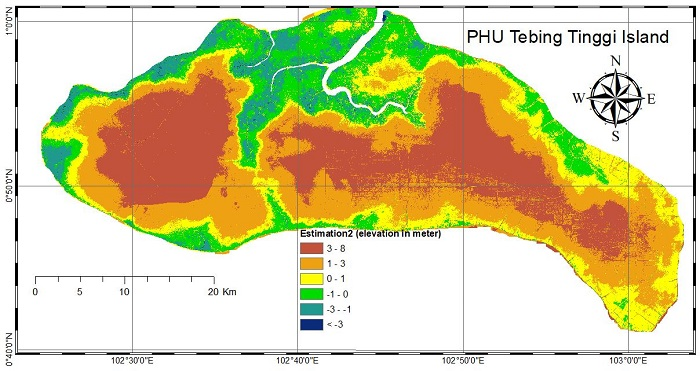
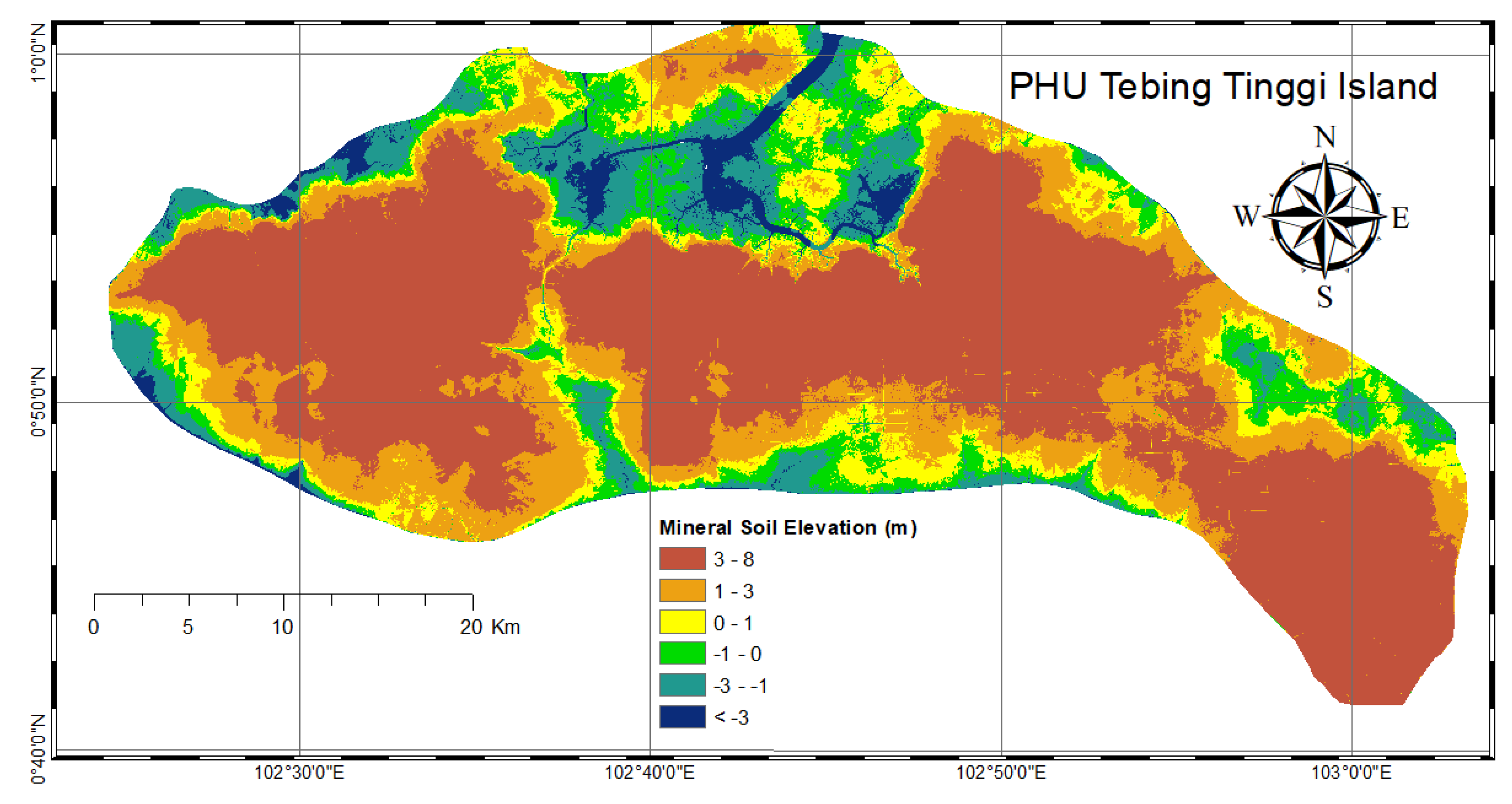
Peat depth drilling data (point data format) were interpolated to be a continuous model for the entire PHU area. That model was then overlaid onto the DTM data to yield the mineral soil position under the peat soil surface. As seen in the mineral soil elevation displayed in Figure 2, mineral soil height varied from –3 m up to 8 m. There were some occurrences of less than 0 m elevation because the peat soil layer in the existing river is thick, and therefore the mineral soil position is far from the ground surface. It may be that the current stream is a new river, which has a different direction than the old one that existed before the formation of this peatland area.
Based on Figure 1 and Figure 2, it can be seen that the residential areas tend to be located in shallow peat areas. The area that has been developed into acacia plantations (south), has a decreased peat depth. It can be compared with the areas of natural forest (west and north-east) the peat conditions that are still relatively thick
3.2. Identification of the Characteristics
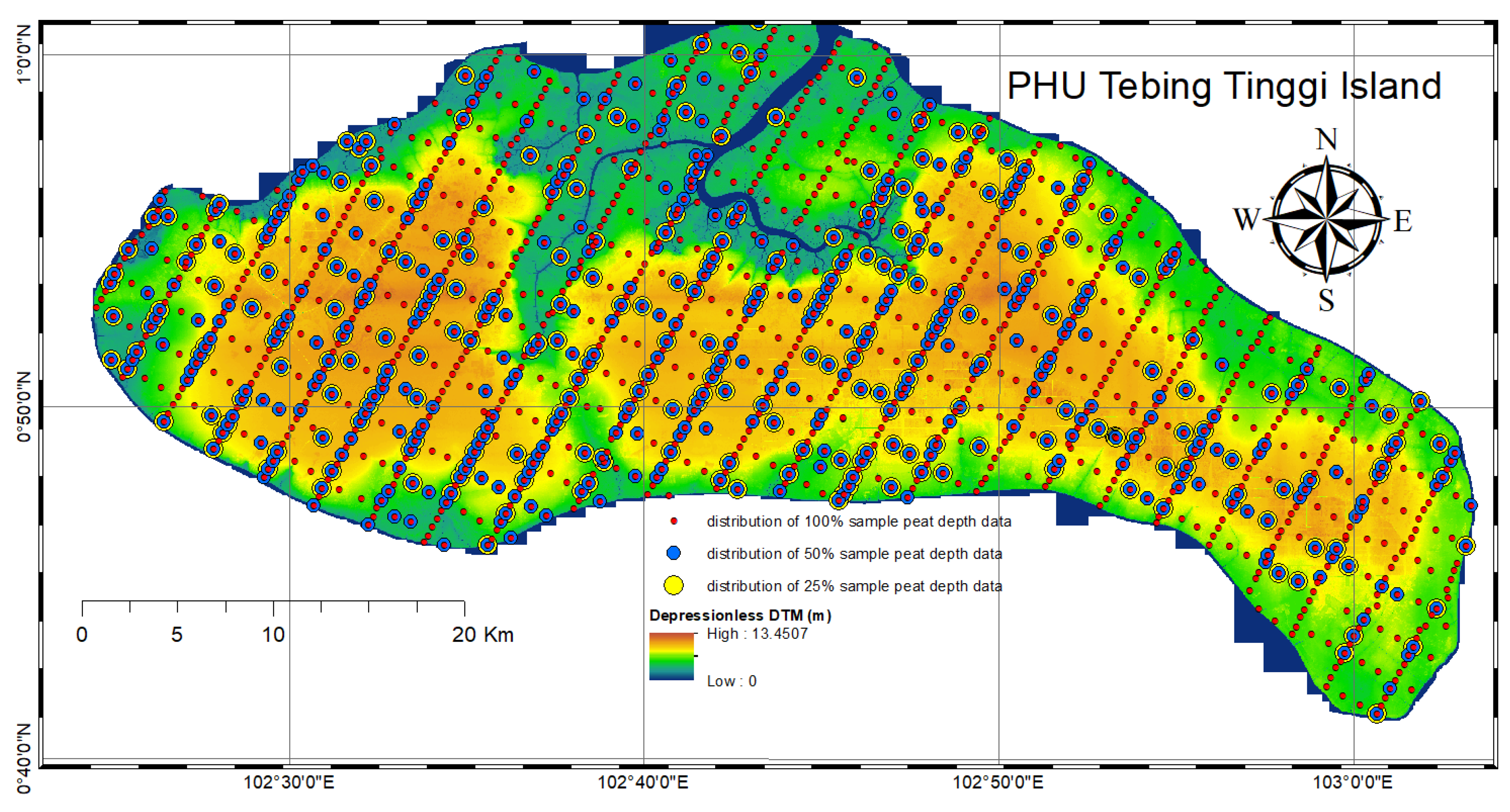
The identification of the peatland properties was conducted by considering certain conditions, which have a relationship with existing peat depth conditions at the location. The identification was performed based on geological, gravitational, and topographical conditions. Some of the data could not be used directly but had to pass through several processing stages in advance. Identifiable characteristics were then used as input parameters (covariates) in the peat depth estimation model. Figure 3 displays the condition of topographic elevation of the entire PHU Tebing Tinggi Island and the distribution of the peat drilling data.
Based on the gravity disturbance condition, it can be seen that the peat dome position could be rapidly identified. When it was compared to the mineral soil condition, it can be observed that there was a similar pattern between mineral soil elevation and this gravity disturbance. Furthermore, geological conditions were dominated by young and older superficial deposits. The pattern of geological conditions had a similar pattern as the surface topography, which showed that there were specific characteristics that affected each other.
Based on the depressionless DTM, a topographical analysis was then carried out. Land slope type (slope position class) and landform class type were determined by following the criteria in [43]. The criteria are determined based on the difference between a cell’s elevation and the average elevation of the neighborhood around that cell. The cell value and the slope of the cell are then classified to define the slope type and landform class type. Based on both types, this PHU area was identified as being very flat. The highest slope area was found only in the riverbank and canals. By identifying landform and slope conditions, it was determined that the trend of peat depth at several locations had changed. By using the depressionless DTM, several characteristics, used as the covariates in peat depth modeling, could also be derived. Those characteristics were valley depth, vertical distance to the channel network, topographic positional index, topographic wetness index, and nearest distance to the river/shoreline.
3.3. Coefficients of Estimation Equation
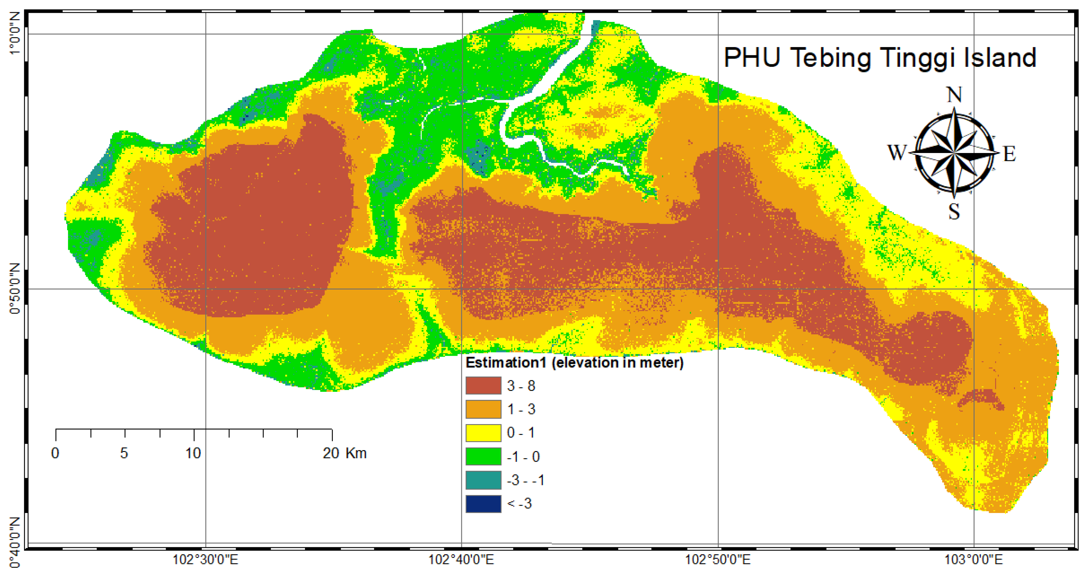
The modeling of the peat depth estimation was carried out based on depressionless DTM, gravity disturbance, geology, slope position index (SPI), landform, valley depth, vertical distance to the channel network, topographic positional index (TPI), topographic wetness index (TWI), and nearest distance to river/shoreline parameters. Peat depth is a distance from the upper peatland (topography) to the upper part of the mineral soil (sub-stratum). Mathematical equation modeling was used to determine the elevation of mineral soil for each raster cell. After knowing the height of the mineral soil of the entire area, peat depth could then be yielded. The OLS was used to gain the coefficient value of each parameter used, as seen in Table 1. In the initial calculation, ten parameters were used involving the whole dataset (defined as estimation 1). The value of the coefficients reflects the effect of each parameter in determining the estimation value of peat depth. Based on results shown in Table 1, it was determined that the parameters of vertical distance to channel network, topographic wetness index, and distance to the nearest river had minimal effects on the equation.
Table 1 also displays the statistical testing results indicating that the parameters of vertical distance to channel network and topographic positional index were less significant in affecting the determination of the estimation equation. This testing was based on the hypothesis that a parameter was considered to significantly affect the peat depth estimation modeling if the value of t-value was greater than 1.96 (confidence level of 95%). When the insignificant parameter was used in mineral soil modeling, the generated peat depth was likely less satisfying. The estimation results of mineral soil elevation by involving all the parameters and input data are displayed in Figure 4.
Based on the generated model, it was determined that gravity data resolution was worse compared with the other data, which also caused the generated model to appear to yield unacceptable results. Although the statistical results showed that the gravity covariate statistically affected the estimation of depth, due to reasons of poor resolution, for the next calculation, this parameter will not be used.
Figure 4 illustrates the geological parameter pattern, which seems more dominant in determining the elevation of mineral soil and peat depth. An obvious gap of peat depth between geological patterns indicated a less logical result. Therefore, the testing result of parameter significance and outliers were considered to generate better results. Elimination of the outliers’ effect for the input data had to be done. The global test was performed by evaluating outliers towards each peat depth drilling result data point. Pope’s Tao testing was also applied to each data point; thereby, it could be identified which of the data were classified as outliers. After reducing the outliers, the coefficients were then recalculated, the results of which are displayed in Table 2 (estimation 2).
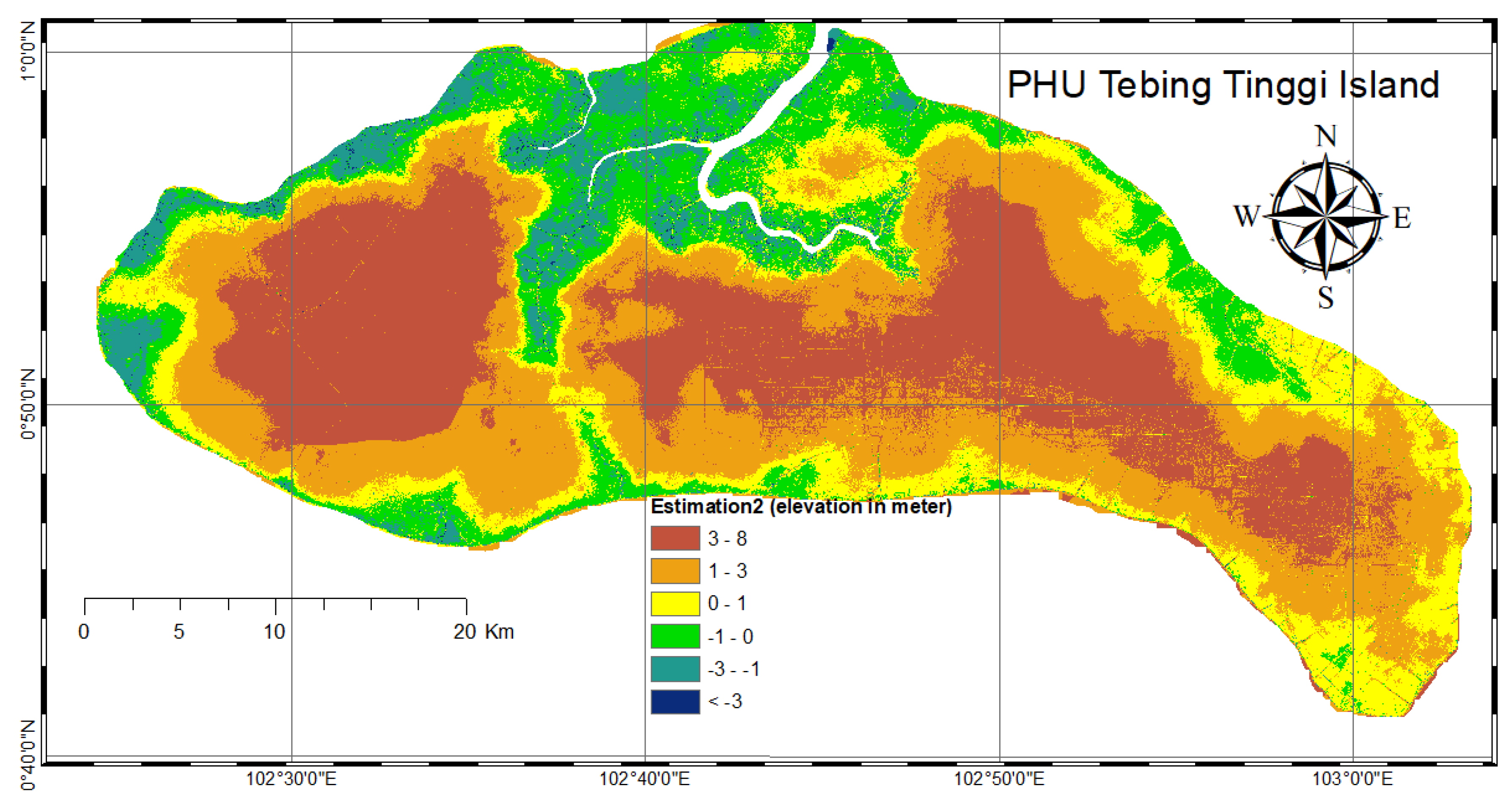
Outliers’ data elimination affected the resulting coefficients. The calculation results, as shown in Table 2, indicated that vertical distance to channel networks and closest distance to river/shoreline covariates were classified as insignificant parameters. Both also had very low coefficient values, which means that the effect of both parameters was minor. All the resulting coefficients shown in Table 2 were then used to calculate the estimated elevation of mineral soil, and the condition of sub-stratum elevation is presented in Figure 5.
Based on Figure 5, the geological pattern is no longer dominantly visible. Generally, the elevation pattern of mineral soil came close to the real mineral soil elevation generated from the field drilling data. As seen in Figure 5, a lengthy pattern from west to east, which has shallow peat, is visible in the center, indicated by the high values of mineral soil elevation. In order to gain more accurate results, the coefficient was re-calculated by ignoring the covariates, which had a small effect and was insignificant in the calculation. The results of the coefficient and significance testing are shown in Table 3 (estimation 3).
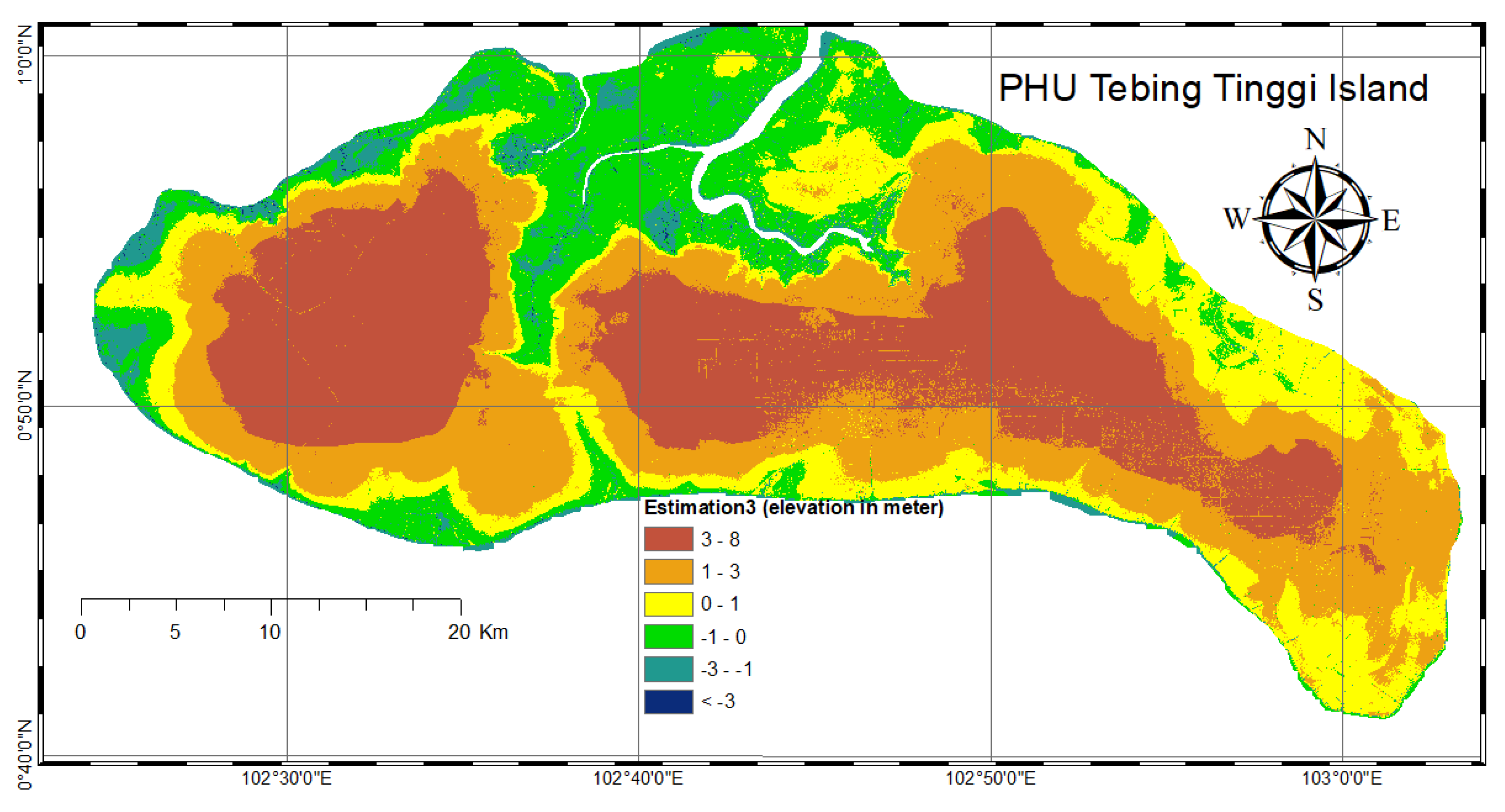
The difference of generated coefficients displayed in Table 3, compared to the Table 1, indicated that those six covariates had a significant effect in estimation modeling, which was shown by all of the significance testing results to those six parameters being accepted by the test. Based on those coefficients, calculation of elevation estimation of mineral soil and peat depth was then carried out. The estimation results of the mineral soil elevation is displayed in Figure 6.
The results of Figure 6, if compared to mineral soil elevation, as displayed in Figure 2, suggest that in general, the height of the mineral soil pattern seen in both figures was almost the same. However, conditions in the northern and eastern coastal areas are relatively different, which are similar to those in the generated model, as shown in Figure 5. The results shown in Figure 6 indicate that ignoring the four covariates causes the geological parameter to become more dominant again; thereby, the geological data pattern emerges in the estimation results. In fact, those eliminated covariates are insignificant, yet the existence of those parameters gives a more realistic result.
3.4. Accuracy Assessments
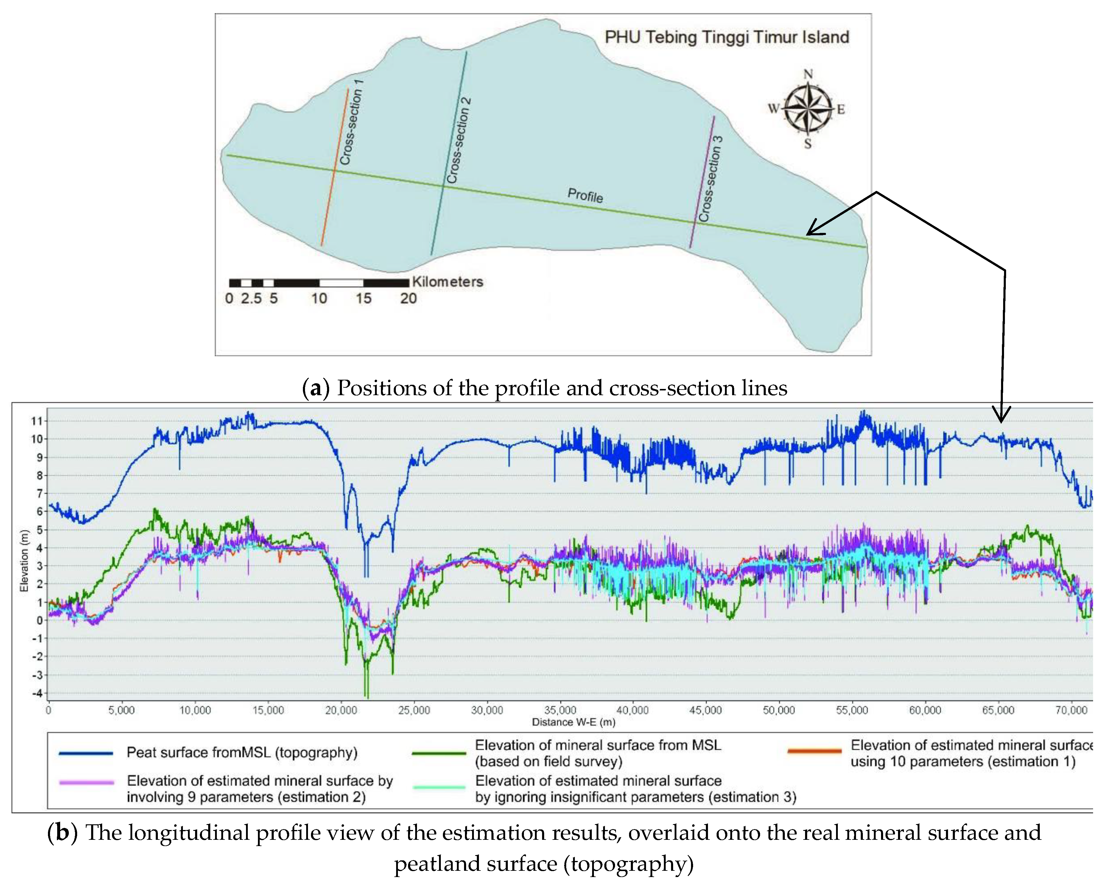
Quality assessment of estimation results was carried out using two approaches: by considering longitudinal profile and cross-sections and by calculating the values of estimation data errors. Profile view identification used four profile & cross-section lines, which consisted of one longitudinal profile and three cross-sections that represented PHU Tebing Tinggi Island. Determination of the location of the profile & cross-sections considers the position of the peat dome in the study area. The profile is assumed to represent the general condition of elevation changing on the PHU Tebing Tinggi Island from west to east. While the cross-section 1 and 3 each represent a cross-section view of the two existing peat domes. Cross-section 2 represents a transitional area between the two existing peat domes. The position of the profile and cross-section line is displayed in Figure 7.
When the resulting estimation models were overlaid onto the real mineral elevation and topography surface, the profile showed the height of each layer, one against the other. Figure 7 shows the peatland depth pattern in the study area displayed with the upper blue line (topography of the peat soil surface) and green line (mineral soil elevation). Generally, mineral soil line patterns can be seen with the estimation 1 result (orange), estimation 2 result (pink), and estimation 3 result (light blue). Based on Figure 7, it can also be seen that in general, there was a deviation between the estimation result and the mineral surface yielded from the field survey.
The estimation 1 (orange) line pattern shows a less suitable trend compared to the real mineral line (green), which is caused by the different resolutions of the input layer. The estimation 2 (pink) profile shows another pattern (compared to estimation 1 and estimation 3), which has the opposite direction to the actual direction of mineral soil elevation. The estimation 3 (light blue) profile is a model result that only involves significant parameters that pass statistical testing. It shows a generally smoother line compared to estimation 1 and estimation 2 patterns. Overall, the generated profile seems to generally follow the real mineral lines. There was some insignificant parameter elimination despite its invisible effect in the numerical calculation. However, it is visible in the profile (pattern).
In order to clarify the quality of the resulting models, several cross-sections were graphed following along the lines of Cross-section 1, Cross-section 2, and Cross-section 3, as seen in Appendix A Figure A1. Based on the deviation value and the tendencies of the mineral soil profile line pattern, it can be concluded that a more realistic result was estimation 2 (pink), which was gained from the equation by calculating all covariates to the equations except for outliers, which were previously eliminated. The estimation result quality was then ensured by comparing estimation result data and the real peat depth data obtained by field drilling. The deviation value results are given in Table 4.
Table 4 shows that outliers’ elimination changed the absolute error value of the calculated data, from 1.237 m in estimation 1 to 1.010 m in estimation 2. Data in estimation 2 and estimation 3 calculations were the same, yet the calculation carried out an elimination of insignificant parameters in determining the coefficient of the elevation estimation equation of mineral soil. Quantitatively, estimation 2 generated better results compared to the other results. The parameters of vertical distance to channel networks, topographic wetness index, and distance to the nearest river did not significantly affect the equation; however, they did in fact affect estimation result patterns. The amount of data used in estimation 1 was higher than in either estimation 2 or estimation 3. This happened because outliers was eliminated by the global test and Baarda’s data snooping; therefore, the number of data points used decreased from 1109 to 971. The amount of collected peat depth drilling data was labor-intensive, meaning that the replication of such method to other PHUs will require enormous labor power, cost, and time.
In order to avoid the need to use large amounts of data, therefore, the next calculation was carried out using decreased data at a rate of 50% and up to 75% of the total dataset. The data selection was carried out randomly but still considered the distribution of the peat drilling positions within the study area. After the selected data (50% and 25% of total data) were obtained, new estimation equations were calculated. The calculation results are displayed in Table 5 (for 50% data) and Table 6 (for 25% data).
By comparing Table 5 and Table 6 to Table 2, it can be seen that the values of the coefficients for the same covariates had different results. It is the characteristic of the OLS method in determining an equation that it calculates each coefficient value based on the condition of the input data. Less data usage causes an increasing number of rejected covariates in statistical testing. This means that the parameters that do not have significant effects on the determination of the estimation equation are increasingly rejected.
Based on the coefficients gained from the OLS calculation, the raster operation was then conducted with nine covariates. Estimation results of mineral soil elevation using 50% peat depth data and 25% data were visually quite similar to the results shown in Table 7. All the estimated mineral models were then compared to each other to assess model quality. The calculation error is displayed in Table 7. In the least-squares adjustment method, calculation error is performed by involving all values in the residual matrix (matrix V). Residual value is the difference between the elevation of mineral soil from the modeling results and the results of field measurements. Then the residual value is calculated statistically to determine the accuracy of the model.
As shown in Table 7, usage of 100% field drilling data with the value of MAE of 1.010 m has the best values compared to others. The usage of 50% data yields the MAE of 1.031 m. The usage of 25% data, the MAE value is 1.020 m, which is slightly better than the 50% data of 11 mm. It was clearly seen that decreasing the number of data points used in the estimation models in fact caused decreased accuracy of the estimation results, which was shown by the decreasing values of MAE from 1.010 to 1.031 m (for 50% data) and 1.020 m (for 25% data). The standard deviation values also increased from 0.755 m to 0.819 m and 0.845 m, respectively, for 50% and 25% data usage.
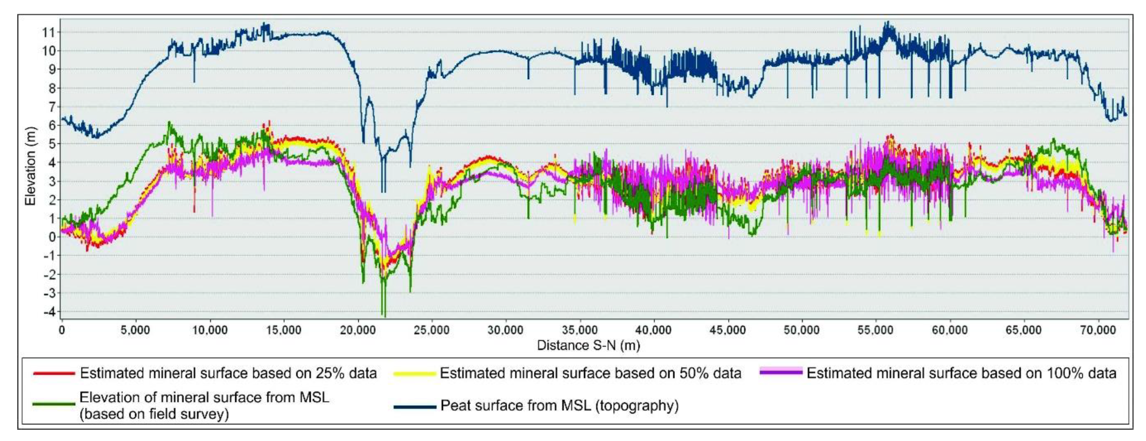
In order to visually check the modelling results, the profile & cross-sections in using 100%, 50%, and 25% of the field data were generated as longitudinal profile and cross-sectional views. The longitudinal profile displayed elevation results based on 25% data (red), 50% data (yellow), and 100% data (pink), as seen in Figure 8. Those results were then overlaid onto topographic data (blue) and the real elevation of mineral soil (green), as seen in Figure 8. Additionally, the cross-sections are shown in Appendix A Figure A2.
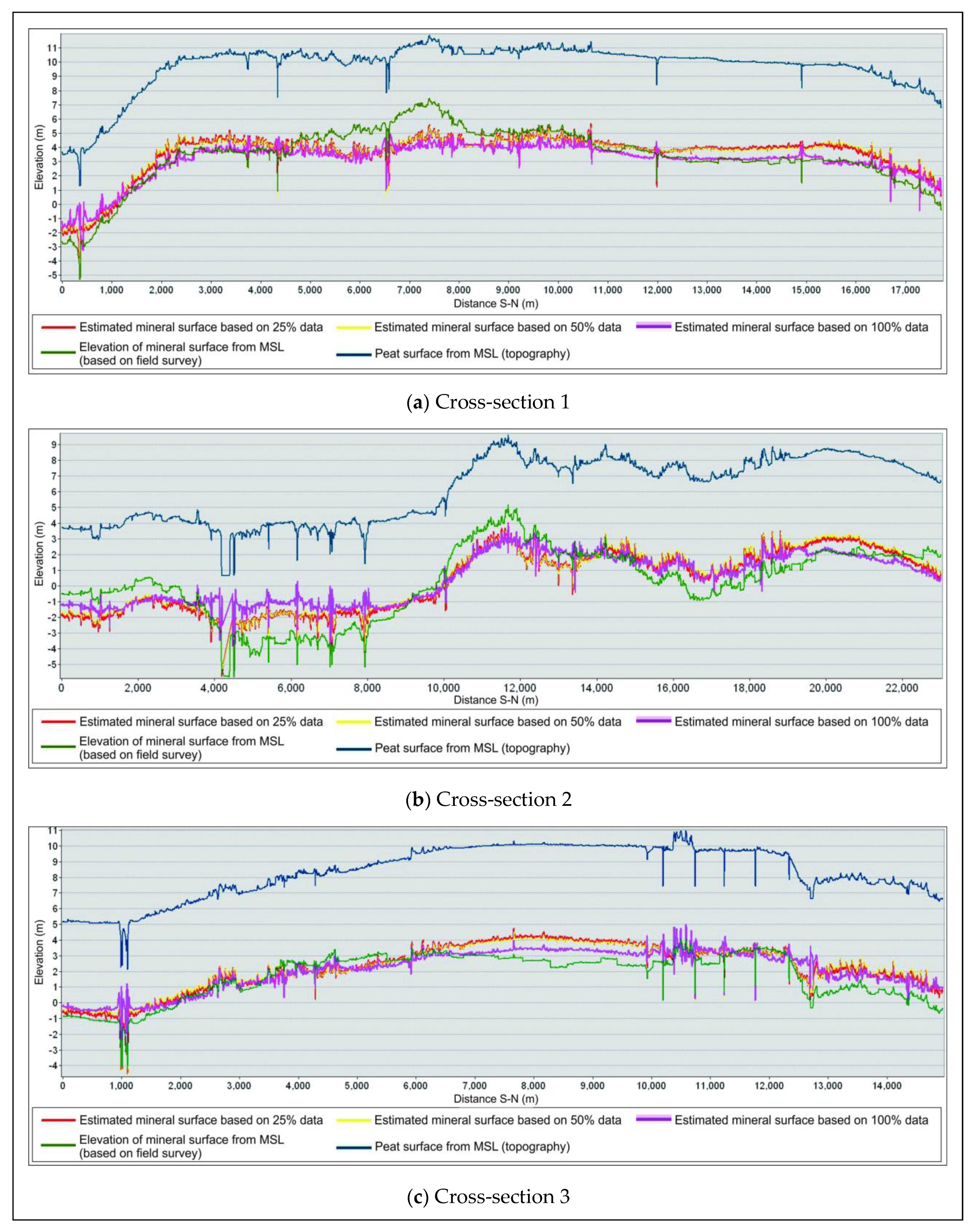
Based on the displayed cross-section in Appendix A Figure A2., it can be seen that the estimation results based on 25% and 50% data had relatively the same pattern. It can be seen that the yellow color (50% data) was closer to the green color (real mineral soil surface). However, when both of them are compared to the estimation results of 100% of the data, it can be inferred that including 100% of the data (which are free from outliers) generates a better cross-section.
Evaluation of the use of 25% and 50% of the data as representative of 100% of the data was then conducted using statistical testing of two variables using confidence intervals of z-tables with a 95% confidence level using Equation (9) as follows [48]:
By involving the data presented in Table 7, the estimation models using 50% of the data showed that the hypothesis was accepted with the value of 0.961 ≤ 1.010 ≤ 1.101. Therefore, statistically, it can be concluded that 50% of data usage still represents use of the entire peat depth dataset with a confidence level of 95% in the mineral elevation modeling. The use of 50% of the data was confirmed statistically using two variable significance testing by Student’s t-test using Equation (10) as follows [48]:
The testing results using Equation (A7) showed that the hypothesis would be accepted if tvalue ≤ ttable. The result for 50% data is tvalue = 0.5001, or less than 1.96. It can be concluded that using 50% of the data in the determination of the estimation equation is statistically the same (insignificantly different) as using the entire dataset (100%) at the confidence level of 95%.
With 25% data usage in the determination of the equation of estimation, it was shown that the results of two variable testing using a z-table with a confidence level of 95% generated the value of 0.920 ≤ 1.010 ≤ 1.120. This means that the statistical testing of two variables showed that using 25% of the data can be representative of the entire dataset. Likewise, the significance testing results generated a tvalue of 0.181 or less than a ttable of 1.96, which confirmed that the use of 25% of the data can be said statistically to be equal to 100% data usage.
The effect of different quality on peat depth data will certainly lead to different calculations of peat volume. The volumetric calculation can be applied to all peat depth models resulted from the OLS method. The volume of the peat depth model can be compared to the real peat volumes calculated based on peat depth probes data, to determine the quality. The results of peat soil volume comparison are presented in the table.
As shown in Table 8, it can be seen that the use of global gravity data, which has a poor spatial resolution, affected more than 11% of distortion of volume calculations from original survey data. It can be confirmed that estimation 2 slightly gave better results than estimation 3 in the peat stock estimation. The number of involved parameters and the amount of data, used in OLS modeling, influence the results of peat soil volume calculations. The percentage difference of the stock estimation between the depth model of 25% of field data and the peat depth model of 50% is 1.02%.
4. Discussion
The utilization of 25% of peat depth data using the OLS method yielded an estimated model which represented the actual conditions on the field. The OLS method is proven to be successful to model very large peatland areas such as in PHU Tebing Tinggi Island which has a total area of 138,748.96 hectares. The peat depth modeling using OLS is able to reduce the involving of peat depth data from 1109 samples, with an ideal density every 500 meters, to 275 data only (see Table 4). Therefore, the selection of sampling strategy becomes crucial to ensure that the distribution and condition of peat samples, as well as their accessibility, are well represented to account for heterogeneity in peat depth [24,30]. The method could be applied to other PHUs in Indonesia, which has 673 PHUs with a total area of 26,477,720 Hectares [49]. In this work, the peat depth estimation using the OLS method is applied to the ombrogenous type of a peatland island.
Compared to the other methods in the modeling of tropical peat depth, the use of the OLS method provides reasonable accuracy. The use of Cubist, Random Forest (RF), and Quantile Regression Forests (QRF) models resulted in RMSE about (≈) 0.6 m for the Ogan Komering Ilir (OKI) area and RMSE ≈ 1.1 m for the Katingan area. The performance of the Artificial Neural Network model is inferior with RMSE = 0.9 m for the OKI area and RMSE = 1.3 m for the Katingan area [24]. Both peatlands (PHU OKI and PHU Katingan) are located on the mainland of Sumatra and Kalimantan, which has different characteristics with a peatland Island like PHU Tebing Tinggi. When the Cubist, RF and QRF methods were applied on a peatland island (Bengkalis), the yielded accuracy of the model is RMSE is 1.8–2.0 m [18].
Land cover conditions have not been used as parameters in peat depth modeling in this paper. In a narrower scope, the condition of land cover and vegetation does not seem to correlate well with the peat depth [14]. However, in a wider scope area of PHU, land use and land cover conditions have an obvious correlation [50]. For this reason, it is necessary to develop the most appropriate scoring method that can represent the correlation between land cover and peat depth. The scoring is essential for qualitative data processing in GIS.
The resulted peat depth model can then be used for various purposes and activities in the context of peat ecosystem restoration. The peat depth model is essential for determining the conservation areas [11,51], and for defining the suitable type and location of canal blockings [52]. The peat depth model is also needed as a basis of evaluation of the carbon stock and the condition the soil organic carbon (SOC) (see e.g., [23,26,53,54]) and is required in the evaluation of peatland ecosystem [55,56], and peatland burn [57,58].
5. Conclusions
The estimation of peat depth can be carried out by subtracting the elevation of the mineral soil layer (as a sub-stratum) from the accurate topographic surface (depressionless DTM). The height of mineral soil can be estimated based on topographical and spatial proximity conditions. In this study, the ordinary least squares adjustment method was used in the estimation equation by involving certain covariates. The covariates used as parameters include depressionless DTM, geological condition, slope position index, landform, valley depth, and vertical distance to channels, topographic positional index, topographic wetness index, and distance to the nearest river. From the statistical testing, we learned that some parameters did not significantly affect the generation of the estimation equation. Nevertheless, the usage of the parameters gave better results in longitudinal profile and cross-sections. Decreasing the number of peat depth drilling data points still resulted in good quality models. Statistical testing carried out to assess the quality showed that the use of 25% and 50% was still representative of all the population of the peat depth data. The accuracies of the generated model, as shown by the values of MAE, were 1.010 m (for 100% data), 1.031 m (for 50% data), and 1.020 m (for 25% data), whereas the standard deviation values were 0.755 m, 0.819 m, and 0.845 m, respectively, for 100%, 50%, and 25% data usage. The result showed that the utilization of the OLS method in peat depth estimation reduced the number of field measurements of peat depth data up to 75% from the normal density. It means that this method improves the efficiency and effectiveness of peat depth mapping, and can be applied to the other PHU. The estimated peat depth model subsequently can be used for several analysis activities in peatland ecosystems. The use of LiDAR data and OLS method offer cost effectiveness for peat depth mapping, expanding beyond its initial purpose for providing high-accuracy topographic data for supporting peat restoration planning and actions.
Author Contributions
Conceptualization, B.K.C., T.A., and I.; methodology, B.K.C.; software, B.K.C.; validation, B.K.C., T.A., and I.; formal analysis, B.K.C.; investigation, B.K.C. and T.A.; data curation, B.K.C.; writing—original draft preparation, B.K.C., T.A., and I.; writing—review and editing, B.K.C. and T.A.; visualization, B.K.C.; supervision, T.A. and I.; project administration, B.K.C.; funding acquisition, T.A. All authors have read and agreed to the published version of the manuscript.
Funding
This work was funded by the Final Project Recognition Program, Universitas Gadjah Mada.
Acknowledgments
We would like to thank the Ministry of Environment and Forestry of the Republic of Indonesia and The Peat Restoration Agency (BRG) for the peat depth data and the LiDAR DTM data; the Universitas Gadjah Mada, for the RTA grant; and the Geodetic Engineering Department for the computer processing facilities. Additionally, we acknowledge Dr. Nurrochmat Widjajanti, Dr. Dwi Lestari, Novi Chiuman, Luthfia Dwi Utami, and Iffati Iffadati for their comments and contributions to the data processing.
Conflicts of Interest
The authors declare no conflict of interest. The funders had no role in the design of the study; in the collection, analyses, or interpretation of data; in the writing of the manuscript; or in the decision to publish the results.
Appendix A
Figure A1.
Cross-section view along the lines of Cross-section 1, Cross-section 2, and Cross-section 3 based on estimation 1, estimation 2, and estimation 3 results, which are overlaid on the real mineral soil surface and peat soil surface (topography).
Figure A1.
Cross-section view along the lines of Cross-section 1, Cross-section 2, and Cross-section 3 based on estimation 1, estimation 2, and estimation 3 results, which are overlaid on the real mineral soil surface and peat soil surface (topography).

Figure A2.
Cross-section view of Cross-section 1, Cross-section 2, and Cross-section 3 lines of mineral soil elevation based on 25%, 50%, and 100% of the data, which are overlaid on the peat surface topography and the real mineral soil elevation.
Figure A2.
Cross-section view of Cross-section 1, Cross-section 2, and Cross-section 3 lines of mineral soil elevation based on 25%, 50%, and 100% of the data, which are overlaid on the peat surface topography and the real mineral soil elevation.

Appendix B
The slope is the first derivative of DTM, which has magnitude and direction. The slope is a vector that consists of gradients and aspects. The term slope is usually also referred to as gradient in geomorphology. The aspect is the direction of the largest slope vector in the tangent plane, which is projected in the horizontal plane, with the slope direction varying from 0o to 360o [59]. The slope usually is used to measure the level of change in elevation and the direction of each change in altitude.
If a plane consists of three points (point 1, point 2, and point 3), where the determination of the slope angle (α) and aspect angle (β) will be measured at point 3. The value of the normal vector of the plane can be determined by Equations (A1) and (A2), while the magnitude of the vector projection in the horizontal plane is calculated by applying Equation (A3). The magnitude of the slope and aspect angles are obtained by applying Equations (A4) and (A5) [59].
The topographic wetness index (TWI) is one of the topographic and hydrological parameters. The concept of TWI was first introduced by Beven and Kirkby [60] as a surface runoff model. The TWI shows the level of wetness of an area. Areas with a higher TWI value tend to be wetter than regions that have a smaller TWI value [44]. The determination of TWI value is strongly influenced by the area of the area above the slope (upslope area) that flows through a certain point per unit length of the contour (A) and the local slope angle (α). So the determination of the wetness index value (TWI) can be calculated based on the following Equation (A6) [61].
This TWI has been used for several applications in hydrological mapping, such as to study the effects of spatial scales on hydrological processes, identification of hydrological flow paths, vegetation patterns, and the quality of forest locations [61].
The identification of relative slope in a certain area can be performed by the relative slope position (RSP) calculations. This RSP represents the slope cell slope position and the relative position between valley elevation and ridge elevation [39]. The relative slope position is calculated for cells in the output grid as the elevation of each cell () relative to the height of the ridge () and valley elevation () as a representation of water flow from top to bottom. The determination of the RSP value is calculated by the following Equation (A7) [39].
Identification of topographic conditions and landforms can be done by determining the topographic position index (TPI). TPI calculation is based on the difference in elevation of a cell to the average elevation of the surrounding area. A positive TPI value indicates that the cell is higher than the surrounding area, while a negative value indicates that the point is located in a valley [43]. The value generated from TPI calculation can be used to classify the slope.
There are 6 classes of slope that can be identified based on these TPI values, namely (1) valley if the TPI value ≤ −1 standard deviation (SD); (2) lower slope if −1 SD <TPI ≤ −0.5 SD; (3) flat slope if −0.5 SD <TPI <0.5 SD and slope ≤ 5°; (4) middle slope if −0.5 SD <TPI <0.5 SD and slope ≤ 5o; (5) upper slope if 0.5 SD <TPI ≤ 1 SD; and (6) ridge if TPI> 1 SD. The class is called the slope position classification [43].
Determination of the output grid size, greatly affects to the value of the resulted TPI. The combination of calculations involving small neighborhood TPI (SN) and large neighborhood TPI (LN) in the calculation of TPI value produce some variation in values. The value obtained turns out to represent the type of landform, which can be categorized in 10 landform classes, namely (1) canyon if TPISN ≤ −1 and TPILN ≤ −1; (2) midslope drainage if TPISN ≤ −1 and −1 < TPILN < −1; (3) upland drainage if TPISN ≤ −1 and TPILN ≥ 1; (4) u-shape valleys if −1 < TPISN < 1 and TPILN ≤ −1; (5) plains if −1 < TPISN < 1 and −1 < TPILN < −1 and slope ≤ 5°; (6) open slope if −1 < TPISN < 1 and −1 < TPILN ≤ 1 and slope > 5°; (7) upper slope if −1 < TPISN < 1 and TPILN ≥ 1; (8) local ridge/hills in valleys if TPISN ≥ 1 and TPILN ≤ −1; (9) midslope ridges, small hills in plains if TPISN ≥ 1 and −1 < TPILN < 1; (10) mountain tops, high ridges if TPISN ≥ 1 and TPILN ≥ 1 [43].
References
- Page, S.E.; Hooijer, A. In the line of fire: The peatlands of Southeast Asia. Philos. Trans. R. Soc. B Biol. Sci. 2016, 371, 20150176. [Google Scholar] [CrossRef] [PubMed] [Green Version]
- Osaki, M.; Tsuji, N. Tropical Peatland Ecosystems; Osaki, M., Tsuji, N., Eds.; Springer: Tokyo, Japan, 2015; ISBN 978-4-431-55681-7. [Google Scholar]
- Jaenicke, J.; Wösten, H.; Budiman, A.; Siegert, F. Planning hydrological restoration of peatlands in Indonesia to mitigate carbon dioxide emissions. Mitig. Adapt. Strateg. Glob. Chang. 2010, 15, 223–239. [Google Scholar] [CrossRef] [Green Version]
- Huijnen, V.; Wooster, M.J.; Kaiser, J.W.; Gaveau, D.L.A.; Flemming, J.; Parrington, M.; Inness, A.; Murdiyarso, D.; Main, B.; van Weele, M. Fire carbon emissions over maritime southeast Asia in 2015 largest since 1997. Nat. Publ. Gr. 2016, 1–8. [Google Scholar] [CrossRef] [PubMed] [Green Version]
- Atwood, E.C.; Englhart, S.; Lorenz, E.; Halle, W.; Wiedemann, W.; Siegert, F.; Atwood, S.; Reid, J.; Kreidenweis, S.; Yu, L.; et al. Detection and Characterization of Low Temperature Peat Fires during the 2015 Fire Catastrophe in Indonesia Using a New High-Sensitivity Fire Monitoring Satellite Sensor (FireBird). PLoS ONE 2016, 11, e0159410. [Google Scholar] [CrossRef] [PubMed] [Green Version]
- Usup, A.; Hashimoto, Y.; Takahasi, H.; Hayasaki, H. Combustion and thermal characteristics of peat fire in tropical peatland in Central Kalimantan, Indonesia. Tropics 2004, 14, 1–19. [Google Scholar] [CrossRef] [Green Version]
- Whittle, A.; Gallego-sala, A.V. Vulnerability of the peatland carbon sink to sea-level rise. Nat. Publ. Gr. 2016, 1–11. [Google Scholar] [CrossRef] [Green Version]
- Dohong, A.; Aziz, A.A.; Dargusch, P. A review of the drivers of tropical peatland degradation in South-East Asia. Land Use policy 2017, 69, 349–360. [Google Scholar] [CrossRef]
- Cattau, M.; Harrison, M.; Defries, R.S. Sources of anthropogenic fire ignitions on the peat-swamp landscape in Kalimantan, Indonesia. Glob. Environ. Chang. 2016, 39, 205–219. [Google Scholar] [CrossRef]
- Jaenicke, J.; Englhart, S.; Siegert, F. Monitoring the effect of restoration measures in Indonesian peatlands by radar satellite imagery. J. Environ. Manag. 2011, 92, 630–638. [Google Scholar] [CrossRef]
- Dohong, A.; Abdul Aziz, A.; Dargusch, P. A Review of Techniques for Effective Tropical Peatland Restoration. Wetlands 2018, 38, 275–292. [Google Scholar] [CrossRef]
- Sekretariat Negara Peraturan Presiden Republik Indonesia Nomor 1 Tahun 2016 Tentang Badan Restorasi Gambut 2016; Sekretariat Negara: Jakarta, Indonesia, 2016; pp. 1–6.
- Jaenicke, J.; Rieley, J.O.; Mott, C.; Kimman, P.; Siegert, F. Determination of the Amount of Carbon Stored in Indonesian Peatlands. Geoderma 2008, 147, 151–158. [Google Scholar] [CrossRef]
- Buffam, I.; Carpenter, S.R.; Yeck, W.; Hanson, P.C.; Turner, M.G. Filling holes in regional carbon budgets: Predicting peat depth in a north temperate lake district. J. Geophys. Res. 2010, 115, 1–16. [Google Scholar] [CrossRef] [Green Version]
- Silvestri, S.; Knight, R.; Viezzoli, A.; Richardson, C.J.; Anshari, G.Z.; Dewar, N.; Flanagan, N.; Comas, X. Quanti fi cation of Peat Thickness and Stored Carbon at the Landscape Scale in Tropical Peatlands: A Comparison of Airborne Geophysics and an Empirical Topographic Method. J. Geophys. Res. Earth Surf. 2019, 124, 3107–3123. [Google Scholar] [CrossRef] [Green Version]
- Keaney, A.; McKinley, J.; Graham, C.; Robinson, M.; Ruffell, A. Spatial statistics to estimate peat thickness using airborne radiometric data. Spat. Stat. 2013, 5, 3–24. [Google Scholar] [CrossRef]
- Parry, L.E.; West, L.J.; Holden, J.; Chapman, P.J. Evaluating Approaches for Estimating Peat Depth. J. Geophys. Res. Biogeosci. 2014, 119, 567–576. [Google Scholar] [CrossRef]
- Rudiyanto Minasny, B.; Setiawan, B.I.; Saptomo, S.K.; McBratney, A.B. Open digital mapping as a cost-effective method for mapping peat thickness and assessing the carbon stock of tropical peatlands. Geoderma 2018, 313, 25–40. [Google Scholar] [CrossRef]
- Jenny, H.; Amundson, R. Factors of Soil Formation A System of Quantitative Pedology, 2nd ed.; Amundson, R., Ed.; Dover Publications, INC.: New York, NY, USA, 1994; ISBN 0486681289. [Google Scholar]
- McBratney, A.B.; Santos, M.L.M.; Minasny, B. On digital soil mapping. Geoderma 2003, 117, 3–52. [Google Scholar] [CrossRef]
- McBratney, A.B.; Minasny, B. Methodologies for Global Soil Mapping; Springer: Dordrecht, The Netherlands, 2010; ISBN 9789048188635. [Google Scholar]
- Young, D.M.; Parry, L.E.; Lee, D.; Ray, S. Spatial models with covariates improve estimates of peat depth in blanket peatlands. PLoS ONE 2018, 13, e0202691. [Google Scholar] [CrossRef] [PubMed]
- Holden, N.M.; Connolly, J. Estimating the carbon stock of a blanket peat region using a peat depth inference model. Catena 2011, 86, 75–85. [Google Scholar] [CrossRef]
- Rudiyanto; Minasny, B.; Setiawan, B.I.; Arif, C.; Saptomo, S.K.; Chadirin, Y. Digital mapping for cost-effective and accurate prediction of the depth and carbon stocks in Indonesian peatlands. Geoderma 2016, 272, 20–31. [Google Scholar] [CrossRef]
- Trisakti, B.; Julzarika, A.; Nugroho, U.C.; Yudhatama, D.; Lasmana, Y. Can the Peat Thickness Classes Be Estimated From Land Cover Type Approach? Int. J. Remote Sens. Earth Sci. 2017, 14, 93. [Google Scholar] [CrossRef] [Green Version]
- Gatis, N.; Luscombe, D.J.; Carless, D.; Parry, L.E.; Fyfe, R.M.; Harrod, T.R.; Brazier, R.E.; Anderson, K. Mapping upland peat depth using airborne radiometric and lidar survey data. Geoderma 2019, 335, 78–87. [Google Scholar] [CrossRef]
- Akpa, S.I.C.; Odeh, I.O.A.; Bishop, T.F.A.; Hartemik, A.E. Digital Mapping of Soil Particle-Size Fractions for Nigeria. Soil Sci. Soc. Am. J. 2014, 78, 1953–1966. [Google Scholar] [CrossRef] [Green Version]
- Millard, K. Development of Methods to Map and Monitor Peatland Ecosystems and Hydrologic Conditions Using Radarsat-2 Synthetic Aperture Radar; Carleton University: Ottawa, ON, Canada, 2016. [Google Scholar]
- Kalacska, M.; Arroyo-Mora, J.P.; Soffer, R.J.; Roulet, N.T.; Moore, T.R.; Humphreys, E.; Leblanc, G.; Lucanus, O.; Inamdar, D. Estimating Peatland water table depth and net ecosystem exchange: A comparison between satellite and airborne imagery. Remote Sens. 2018, 10, 687. [Google Scholar] [CrossRef] [Green Version]
- Parry, L.E.; Charman, D.J.; Noades, J.P.W. A method for modelling peat depth in blanket peatlands. Soil Use Manag. 2012, 28, 614–624. [Google Scholar] [CrossRef]
- Zainorabidin, A.; Wijeyesekera, D.C. Geotechnical Challeges with Malaysian Peat. In Proceedings of the 2nd Annual Conference of the Advances Computing and Technology, London, UK, 23 January 2007; pp. 252–261. [Google Scholar]
- Barthelmes, F. Definition of Functionals of the Geopotential and Their Calculation from Spherical Harmonic Models; The International Centre for Global Earth Models (ICGEM) GeoForschungsZentrum (GFZ): Potsdam, Germany, 2013. [Google Scholar]
- Kasenda, A. High Precision Geoid for Modernization of Height System in Indonesia; The University of New South Wales: Sydney, Australia, 2009. [Google Scholar]
- Sideris, M.G.; Editor, S. Proceedings of the International Association of Geodesy Symposia, IAG 2011, Munich, Germany, 13–15 April 2011; Springer: Berlin, Germany; Volume 139, ISBN 9783642372216.
- Thenkabail, P.S.; Lyon, J.G.; Huete, A. Hyperspectral Remote Sensing of Vegetation and Agricultural Crops: Knowledge Gain and Knowledge Gap After 40 Years of Research. In Hyperspectral Remote Sensing of Vegetation; Taylor & Francis Group: Abingdon, UK, 2010; pp. 663–688. [Google Scholar]
- McBratney, A.B.; Minasny, B. Methodologies for Global Soil Mapping. In Digital Soil Mapping, Progress in Soil Science 2; Springer Science: Dordrecht, The Netherlands, 2010; pp. 429–436. ISBN 9789048188635. [Google Scholar]
- Sinem Ince, E.; Barthelmes, F.; Reißland, S.; Elger, K.; Förste, C.; Flechtner, F.; Schuh, H. ICGEM—15 years of successful collection and distribution of global gravitational models, associated services, and future plans. Earth Syst. Sci. Data 2019, 11, 647–674. [Google Scholar] [CrossRef] [Green Version]
- Badan Restorasi Gambut. Peatland Mapping of 23 Hydrological Units; Badan Restorasi Gambut: Jakarta, Indonesia, 2019. [Google Scholar]
- Conrad, O.; Bechtel, B.; Bock, M.; Dietrich, H.; Fischer, E.; Gerlitz, L.; Wehberg, J.; Wichmann, V.; Böhner, J. System for Automated Geoscientific Analyses (SAGA) v. 2.1.4. Geosci. Model Dev. 2015, 8, 1991–2007. [Google Scholar] [CrossRef] [Green Version]
- Lindsay, J.B.; Creed, I.F. Removal of artifact depressions from digital elevation models: Towards a minimum impact approach. Hydrol. Process. 2005, 19, 3113–3126. [Google Scholar] [CrossRef]
- Kiamehr, R.; Sjöberg, L.E. Impact of a precise geoid model in studying tectonic structures-A case study in Iran. J. Geodyn. 2006, 42, 1–11. [Google Scholar] [CrossRef]
- Jenson, S.K.; Domingue, J.O. Extracting topographic structure from digital elevation data for geographic information system analysis. Photogramm. Eng. Remote Sensing 1988, 54, 1593–1600. [Google Scholar]
- Jenness, J. Topographic Position Index; Jenness Enterprises: Flagstaff, AZ, USA, 2006. [Google Scholar]
- Lang, M.; McCarty, G.; Oesterling, R.; Yeo, I.Y. Topographic metrics for improved mapping of forested wetlands. Wetlands 2013, 33, 141–155. [Google Scholar] [CrossRef]
- Esterle, J.S.; Ferm, J.C. Spatial variability in modern tropical peat deposits from Sarawak, Malaysia and Sumatra, Indonesia: Analogues for coal. Int. J. Coal Geol. 1994, 26, 1–41. [Google Scholar] [CrossRef]
- Enki Yoo, E.-H.; Aldstadt, J.; Shi, W. Principles of Modeling Uncertainties in Spatial Data and Spatial Analyses; CRC Press: Boca Raton, FL, USA, 2011; Volume 51, ISBN 9781420059274. [Google Scholar]
- Ghilani, C.D. Adjustment Computations, 6th ed.; John Wiley & Sons, Inc.: Hoboken, NJ, USA, 2017; ISBN 9781119385981. [Google Scholar]
- Leick, A.; Rapoport, L.; Tatarnikov, D. GPS Satellite Surveying, 4th ed.; John Wiley & Sons, Inc.: Hoboken, NJ, USA, 2015; ISBN 9781118675571. [Google Scholar]
- Directorate of Peat Degradation Control. Map of Indonesia Peat Hydrological Units; The Ministry of Environment and Forestry Republic of Indonesia: Jakarta, Indonesia, 2017.
- Lopatin, J.; Kattenborn, T.; Galleguillos, M.; Perez-Quezada, J.F.; Schmidtlein, S. Using aboveground vegetation attributes as proxies for mapping peatland belowground carbon stocks. Remote Sens. Environ. 2019, 231, 111217. [Google Scholar] [CrossRef]
- Grand-Clement, E.; Anderson, K.; Smith, D.; Angus, M.; Luscombe, D.J.J.; Gatis, N.; Bray, L.S.S.; Brazier, R.E.E. New approaches to the restoration of shallow marginal peatlands. J. Environ. Manag. 2015, 161, 417–430. [Google Scholar] [CrossRef] [PubMed] [Green Version]
- Bragg, O.; Lindsay, R.; Risager, M.; Silvius, M.; Zingstra, H. Strategy and Action Plan for Mire and Peatland Conservation in Central Europe; Wetlands International: Wageningen, The Netherlands, 2003. [Google Scholar]
- Chapman, S.J.; Bell, J.; Donnelly, D.; Lilly, A. Carbon stocks in Scottish peatlands. Soil Use Manag. 2009, 25, 105–112. [Google Scholar] [CrossRef]
- Rudiyanto; Setiawan, B.I.; Arif, C.; Saptomo, S.K.; Gunawan, A.; Kuswarman, S.; Indriyanto, H. Estimating Distribution Of Carbon Stock In Tropical Peatland Using A Combination Of An Empirical Peat Depth Model And GIS. In Proceedings of the The 1st International Symposium on LAPAN-IPB Satellite for Security and Environmental Monitoring; Procedia Environmental Science, 2015, Bogor, Indonesia, 25–26 November 2014; pp. 152–157. [Google Scholar]
- Waddington, J.M.; Kellner, E.; Strack, M.; Price, J.S. Differential peat deformation, compressibility, and water storage between peatland microforms: Implications for ecosystem function and development. Water Resour. Res. 2010, 46, 1–12. [Google Scholar] [CrossRef]
- Joosten, H.; Tapio-Biström, M.-L.; Tol, S. Peatlands—Guidance for Climate Change Mitigation through Conservation, Rehabilitation, 5th ed.; FAO of the UN and Wetlands International: Rome, Italy, 2012; ISBN 9789251073025. [Google Scholar]
- Simpson, J.E.; Wooster, M.J.; Smith, T.E.L.; Trivedi, M.; Vernimmen, R.R.E.; Dedi, R.; Shakti, M.; Dinata, Y. Tropical peatland burn depth and combustion heterogeneity assessed using uav photogrammetry and airborne LiDAR. Remote Sens. 2016, 8, 1000. [Google Scholar] [CrossRef] [Green Version]
- Ballhorn, U.; Siegert, F.; Mason, M.; Limin, S. Derivation of burn scar depths and estimation of carbon emissions with LIDAR in Indonesian peatlands. Proc. Natl. Acad. Sci. USA 2009, 106, 21213–21218. [Google Scholar] [CrossRef] [Green Version]
- Li, Z.; Zhu, Q.; Gold, C. Digital terrain modeling: Principles and methodology, 1st ed.; CRC Press: Boca Raton, FL, USA, 2004; ISBN 0-415-32462-9. [Google Scholar]
- Beven, K.J.; Kirkby, M.J. A physically based, variable contributing area model of basin hydrology. Hydrol. Sci. Bull. 1979, 24, 43–69. [Google Scholar] [CrossRef] [Green Version]
- Sørensen, R.; Zinko, U.; Seibert, J. On the calculation of the topographic wetness index: Evaluation of different methods based on field observations. Hydrol. Earth Syst. Sci. 2006, 10, 101–112. [Google Scholar] [CrossRef] [Green Version]
Figure 1.
Aerial photograph visualization of the Peat Hydrological Unit (PHU) area of Tebing Tinggi Island with the river and stream (blue line) and street features (red line) added.
Figure 1.
Aerial photograph visualization of the Peat Hydrological Unit (PHU) area of Tebing Tinggi Island with the river and stream (blue line) and street features (red line) added.

Figure 2.
Mineral Soil Elevation above the local Mean Sea Level (MSL).

Figure 3.
Condition of topographic (depressionless digital terrain model (DTM) above the local MSL) and distribution of peat measurements on file.
Figure 3.
Condition of topographic (depressionless digital terrain model (DTM) above the local MSL) and distribution of peat measurements on file.

Figure 4.
The condition of elevation mineral soil resulted in the estimation model by involving all covariates. Note: the elevation is above the local MSL.
Figure 4.
The condition of elevation mineral soil resulted in the estimation model by involving all covariates. Note: the elevation is above the local MSL.

Figure 5.
Mineral soil position of estimation results by ignoring gravity parameters and outliers. Note: the elevation is above the local MSL.
Figure 5.
Mineral soil position of estimation results by ignoring gravity parameters and outliers. Note: the elevation is above the local MSL.

Figure 6.
Estimation results of the mineral soil elevation after eliminating four insignificant parameters and removing outliers. Note: the elevation is above the local MSL.
Figure 6.
Estimation results of the mineral soil elevation after eliminating four insignificant parameters and removing outliers. Note: the elevation is above the local MSL.

Figure 7.
(a) Positions of the profile line and (b) the longitudinal profile view along the profile line. Note: cross-section 1, cross-section 2, and cross section 3 can be seen in Appendix A.
Figure 7.
(a) Positions of the profile line and (b) the longitudinal profile view along the profile line. Note: cross-section 1, cross-section 2, and cross section 3 can be seen in Appendix A.

Figure 8.
Longitudinal profile of the estimation results of mineral soil elevation based on 25%, 50%, and 100% of data, which are overlaid onto the peat surface topography and the real mineral soil elevation.
Figure 8.
Longitudinal profile of the estimation results of mineral soil elevation based on 25%, 50%, and 100% of data, which are overlaid onto the peat surface topography and the real mineral soil elevation.


Table 1.
The calculation results of the coefficients by involving the entire dataset and all the parameters (estimation 1). Digital terrain model (DTM); slope position index (SPI); topographic positional index (TPI); topographic wetness index (TWI); standard deviation (SD).
Table 1.
The calculation results of the coefficients by involving the entire dataset and all the parameters (estimation 1). Digital terrain model (DTM); slope position index (SPI); topographic positional index (TPI); topographic wetness index (TWI); standard deviation (SD).
| Covariates | DTM | Gravity | Geology | SPI | Landform | Valley Depth | Vertical Distance | TPI | TWI | Nearest River | Constant |
|---|---|---|---|---|---|---|---|---|---|---|---|
| coefficient | 0.5326 | –0.1907 | –0.2993 | –1.09 | 0.4473 | 0.3322 | –0.0759 | 0.1952 | –0.0774 | –0.0165 | 10.942 |
| SD | 0.0208 | 0.0576 | 0.0264 | 0.1366 | 0.1199 | 0.0855 | 0.0523 | 0.1665 | 0.0149 | 0.0041 | 0.3652 |
| t-value | 25.6612 | –3.3086 | –11.3404 | –7.9821 | 3.7321 | 3.8863 | –1.4505 | 1.1722 | –5.1931 | –4.0165 | 29.9605 |
Note: a significance level of α = 0.05, and the value of t-table is 1.96.
Table 2.
The calculation results of the coefficient after eliminating gravity disturbance and outliers from the input data (estimation 2).
Table 2.
The calculation results of the coefficient after eliminating gravity disturbance and outliers from the input data (estimation 2).
| Covariates | DTM | Geology | SPI | Land Form | Valley Depth | Vertical Distance | TPI | TWI | Nearest River | Constant |
|---|---|---|---|---|---|---|---|---|---|---|
| Coefficient | 0.60140 | −0.24190 | −1.12370 | 0.50380 | 0.37550 | −0.03160 | 0.33200 | −0.05260 | 0.00760 | 7.13670 |
| SD | 0.0176 | 0.0279 | 0.1407 | 0.1352 | 0.0951 | 0.056 | 0.1662 | 0.0158 | 0.0044 | 0.4681 |
| t-value | 34.2421 | −8.6556 | −7.9886 | 3.7269 | 3.9467 | −0.5641 | 1.9976 | −3.3244 | 1.7253 | 15.2467 |
Note: a significance level of α = 0.05, and the value of t-table is 1.96.
Table 3.
Results of the coefficients and t-value by eliminating insignificant covariates and small effect parameters in the equation (estimation 3).
Table 3.
Results of the coefficients and t-value by eliminating insignificant covariates and small effect parameters in the equation (estimation 3).
| Covariates | DTM | Geology | SPI | Land Form | Valley Depth | TPI | Constant |
|---|---|---|---|---|---|---|---|
| Coefficient | 0.61340 | −0.22890 | −1.20190 | 0.60600 | 0.36950 | 0.45970 | 5.74200 |
| SD | 0.0156 | 0.0265 | 0.1402 | 0.1339 | 0.0926 | 0.1576 | 0.4948 |
| t-value | 39.3077 | −8.6298 | −8.5718 | 4.5265 | 3.9887 | 2.9172 | 11.6053 |
Note: a significance level of α = 0.05, and the value of t-table is 1.96.
Table 4.
Error Calculation of the different elevation between the real mineral soil line and the estimation results. Mean absolute error (MAE); minimum error (min error); maximum error (max error).
Table 4.
Error Calculation of the different elevation between the real mineral soil line and the estimation results. Mean absolute error (MAE); minimum error (min error); maximum error (max error).
| Estimation 1 | Estimation 2 | Estimation 3 | |
|---|---|---|---|
| MAE | 1.237 m | 1.010 m | 1.019 m |
| Min Error | 0.002 m | 0.004 m | 0.002 m |
| Max Error | 5.181 m | 3.614 m | 3.675 m |
| SD | 1.076 m | 0.755 m | 0.746 m |
| total data | 1109 | 971 | 971 |
Table 5.
Coefficient calculation results using 50% data.
| Covariates | DTM | Geology | SPI | Land Form | Valley Depth | Vertical Distance | TPI | TWI | NearestRiver | Constant |
|---|---|---|---|---|---|---|---|---|---|---|
| Coefficient | 0.898 | 0.1037 | −0.5354 | 0.0159 | 0.0011 | −0.0447 | 0.8892 | −0.0168 | 0.263 | 1.7769 |
| SD | 0.0233 | 0.0365 | 0.2164 | 0.1882 | 0.1106 | 0.0787 | 0.206 | 0.0214 | 0.0558 | 0.4445 |
| t-value | 38.5058 | 2.843 | −2.474 | 0.0845 | 0.01 | −0.5679 | 4.3165 | −0.7841 | 4.7151 | 3.9978 |
Note: a significance level of α = 0.05, and the value of t-table is 1.96.
Table 6.
The calculation results of coefficients using 25% data.
| Covariates | DTM | Geology | SPI | Land Form | Valley Depth | Vertical Distance | TPI | TWI | NearestRiver | Constant |
|---|---|---|---|---|---|---|---|---|---|---|
| coefficient | 0.8829 | 0.0141 | −0.4958 | −0.3635 | −0.0062 | −0.0836 | 1.3446 | −0.0249 | 0.3111 | −8.2318 |
| SD | 0.0332 | 0.0508 | 0.3121 | 0.3281 | 0.1737 | 0.1069 | 0.2925 | 0.0321 | 0.0772 | 0.3071 |
| t-value | −26.5681 | −0.2775 | 1.5885 | 1.1077 | 0.0355 | 0.7825 | −4.5964 | 0.7776 | −4.0291 | 26.8033 |
Note: a significance level of α = 0.05, and the value of t-table is 1.96.
Table 7.
Accuracy assessment of estimated data using 100%, 50%, and 25% data of field peat depth.
| 100% Data | 50% Data | 25% Data | |
|---|---|---|---|
| MAE | 1.010 m | 1.031 m | 1.020 m |
| Min Error | 0.004 m | 0.001 m | 0.001 m |
| Max Error | 3.614 m | 4.700 m | 4.688 m |
| SD | 0.755 m | 0.819 m | 0.845 m |
| total data | 971 | 524 | 274 |
Table 8.
Volume comparison between the models resulted from the ordinary least square (OLS) method and the filed measurement.
Table 8.
Volume comparison between the models resulted from the ordinary least square (OLS) method and the filed measurement.
| Data | Volume (m3) | Δ vol (%) |
|---|---|---|
| peat volume (original peat depth probe) | 8,299,347,092.475 | |
| Δ vol. peat-probe vs. estimation1 | - 933,186,413.099 | 11.244 |
| Δ vol. peat-probe vs. estimation2 | - 567,061,186.697 | 6.833 |
| Δ vol. peat-probe vs. estimation3 | - 636,868,262.057 | 7.674 |
| Δ vol. peat-probe vs. 50% data | - 542,225,677.094 | 6.533 |
| Δ vol. peat-probe vs. 25% data | - 627,199,328.081 | 7.557 |
© 2020 by the authors. Licensee MDPI, Basel, Switzerland. This article is an open access article distributed under the terms and conditions of the Creative Commons Attribution (CC BY) license (http://creativecommons.org/licenses/by/4.0/).
Share and Cite
MDPI and ACS Style
Cahyono, B.K.; Aditya, T.; Istarno. The Least Square Adjustment for Estimating the Tropical Peat Depth Using LiDAR Data. Remote Sens. 2020, 12, 875. https://0-doi-org.brum.beds.ac.uk/10.3390/rs12050875
AMA Style
Cahyono BK, Aditya T, Istarno. The Least Square Adjustment for Estimating the Tropical Peat Depth Using LiDAR Data. Remote Sensing. 2020; 12(5):875. https://0-doi-org.brum.beds.ac.uk/10.3390/rs12050875
Chicago/Turabian StyleCahyono, Bambang Kun, Trias Aditya, and Istarno. 2020. "The Least Square Adjustment for Estimating the Tropical Peat Depth Using LiDAR Data" Remote Sensing 12, no. 5: 875. https://0-doi-org.brum.beds.ac.uk/10.3390/rs12050875
Note that from the first issue of 2016, this journal uses article numbers instead of page numbers. See further details here.