Accuracy Verification of Airborne Large-Footprint Lidar based on Terrain Features


1
State Key Laboratory of Information Engineering in Surveying, Mapping and Remote Sensing, Wuhan University, Wuhan 430079, China
2
Beijing Institute of Tracking and Communication Technology, Beijing 100094, China
3
China Siwei Surveying and Mapping Technology Co. Ltd., Beijing 100094, China
4
China Centre For Resources Satellite Data and Application, Beijing 100094, China
*
Author to whom correspondence should be addressed.
Remote Sens. 2020, 12(5), 879; https://0-doi-org.brum.beds.ac.uk/10.3390/rs12050879
Submission received: 15 January 2020
/
Revised: 26 February 2020
/
Accepted: 7 March 2020
/
Published: 9 March 2020
Abstract
:Accuracy verification of airborne large-footprint lidar data is important for proper data application but is difficult when ground-based laser detectors are not available. Therefore, we developed a novel method for lidar accuracy verification based on the broadened echo pulse caused by signal saturation over water. When an aircraft trajectory crosses both water and land, this phenomenon and the change in elevation between land and water surfaces can be used to verify the plane and elevation accuracy of the airborne large-footprint lidar data in conjunction with a digital surface model (DSM). Due to the problem of echo pulse broadening, the center-of-gravity (COG) method was proposed to optimize the processing flow. We conducted a series of experiments on terrain features (i.e., the intersection between water and land) in Xiangxi, Hunan Province, China. Verification results show that the elevation accuracy obtained in our experiments was better than 1 m and the plane accuracy was better than 5 m, which is well within the design requirements. Although this method requires specific terrain conditions for optimum applicability, the results can lead to valuable improvements in the flexibility and quality of lidar data collection.

1. Introduction
Light detection and ranging (lidar) integrates laser technology, the global positioning system (GPS), and the inertial navigation system (INS) into a highly accurate measurement system. Lidar can be divided into small-footprint systems that discretely record a small amount of echo data in higher detail, and large-footprint (8–70 m) systems that record complete waveforms over a broader range, which exhibit greater ability to penetrate vegetative canopies but have relatively lower resolution [1]. The latter allows accurate measurements of surface information at larger scales and plays an important role in polar ice sheet measurement, vegetation height inversion, biomass estimation, and other fields [2,3,4,5,6]. The development of large-footprint lidar has been led by the United States and includes NASA’s airborne Laser Vegetation Imaging Sensor (LVIS) [7,8], Scanning Lidar Imager of Canopies by Echo Recovery (SLICER) [9], and spaceborne Geoscience Laser Altimeter System (GLAS) systems [10,11,12]. Other countries have been working to improve their own capabilities. For example, Japan launched the lunar satellite with the Lunar Orbiter Laser Altimeter (LOLA) in 2007 [13], and China launched the ZiYuan3-02 (ZY3-02) satellite in May 2016 (the first experimental satellite payload equipped with a laser altimeter for Earth observation) [14] and the GaoFen-7 (GF-7) satellite in November 2019 (the first formal spaceborne laser altimeter equipped for global stereo mapping) [15].
Geometrical precision is an important index for measuring laser performance. Errors in large-footprint lidar data, which are the main factors affecting positioning accuracy, are predominantly caused by hardware issues, atmospheric refraction, topographic variations, and the influence of ground features [14]. Properly evaluating the positioning accuracy of large-footprint lidar can ensure data quality and optimal performance when using new instrumentation. At present, there are two verification methods for large-footprint lidar. One deploys laser detectors and the other involves waveform matching between the laser echo simulated by a high-precision digital surface model (DSM) and the actual laser echo. Some studies have attempted to address this issue by arranging infrared signal detectors on the ground surface [16,17,18,19]. Others have used the unique signal generated in the reflected wave by the corner cube retroreflector (CCR) to obtain time information for calibrating synchronization errors [20,21]. To verify the accuracy of the ZY3-02 satellite, a detector was set up in the Gobi Desert (Inner Mongolia) to capture laser footprint energy [14,22,23]. Moreover, previous research matched simulated waveforms with actual waveforms to verify laser pointing and ranging errors in California and Antarctica [24,25]. These methods are reliable, stable, and suitable for the verification of satellite lidar. However, the deployment of laser detectors is time-consuming and labor-intensive; thus, it is not practical for airborne lidar work with a narrower and more variable focus. The method of waveform matching results in highly accurate distance verification; however, it has limited plane accuracy verification ability, and its effect is not ideal when the transmitted signal cannot reflect the true energy distribution. Therefore, flexible and efficient methods are required to verify the elevation and plane accuracy of airborne large-footprint lidar.
At the water–land intersection, the echo waveforms of the water will exhibit peak clipping and pulse broadening due to signal saturation [26], resulting in the echo waveform of the two terrains displaying different characteristics (the water waveform is saturated, whereas the land waveform is unsaturated). There will also be a distinct elevation difference between the two. In this study, we developed a method that uses the difference of the waveform and the elevation at the water–land intersection to verify the elevation and plane accuracy of airborne lidar data without laser detectors, ensuring data quality, while remaining flexible and rapid. However, when processing the saturated waveform of the water, the traditional approach, which uses the Gaussian fitting method, will result in a lower measured elevation. As our accuracy verification method relies on the positioning accuracy of the water surface, we propose a center-of-gravity (COG) method for the data processing to optimize the saturation problem. We then test this accuracy verification approach using lidar data collected in Xiangxi, Hunan Province, China.
2. Materials and Methods
2.1. Experimental Study Area and Data Sources
The study area is located in Xiangxi, northwestern Hunan Province, China (109.35–111.33° E, 28.11–29.21° N). This region lies within the Yunnan–Guizhou Plateau, with a complex terrain surrounded by mountains and crossed by rivers, and contains a variety of features, including towns and farmland. The experiment was conducted in December 2017, when there was a clear sky and low cloud cover.
2.1.1. Large-footprint Lidar Data
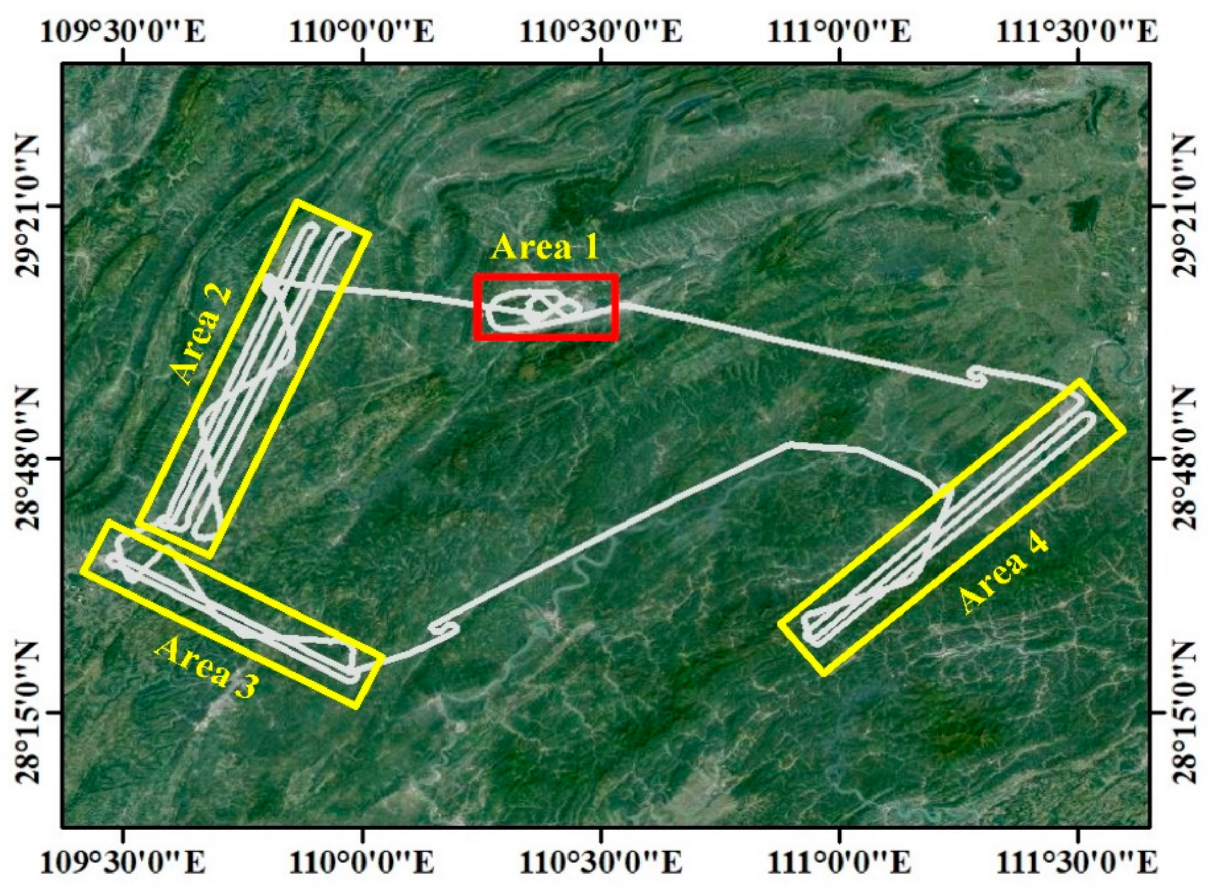
We used lidar data from China’s first airborne forestry detection large-footprint lidar system (designed by the State Forestry Administration of China [27,28]). The technical parameters are given in Table 1. The laser was emitted at a 3-km altitude, with a footprint spot diameter of ~15 m and spacing of ~1.8 m at ground level. Our experimental design requires that the elevation accuracy is better than 1 m and the positioning accuracy is better than 5 m. The flight route covered four measurement areas with a total of 37 tracks (Figure 1). Area 1 was used to verify the elevation accuracy and Areas 2–4 were used to verify the plane accuracy.
2.1.2. Other Data
To generate the DSM data used to assist accuracy verification, we conducted eight flights of small-footprint lidar (Leica ALS70HP) in the study areas during the performance of the airborne large-footprint lidar experiment. DSM data with a resolution of 0.5 m was generated for Area 1 to verify the accuracy of large-footprint lidar data elevation measurement, and DSM data with a resolution of 2 m was used for Areas 2, 3, and 4 to verify the accuracy of large-footprint lidar data plane positioning. We used GF-2 satellite imagery (with a resolution of 0.8 m) for visual assessment and verification of the large-footprint lidar data. Position and orientation system (POS) data included time, attitude, position, speed, and other information for geometric positioning of the lidar data.
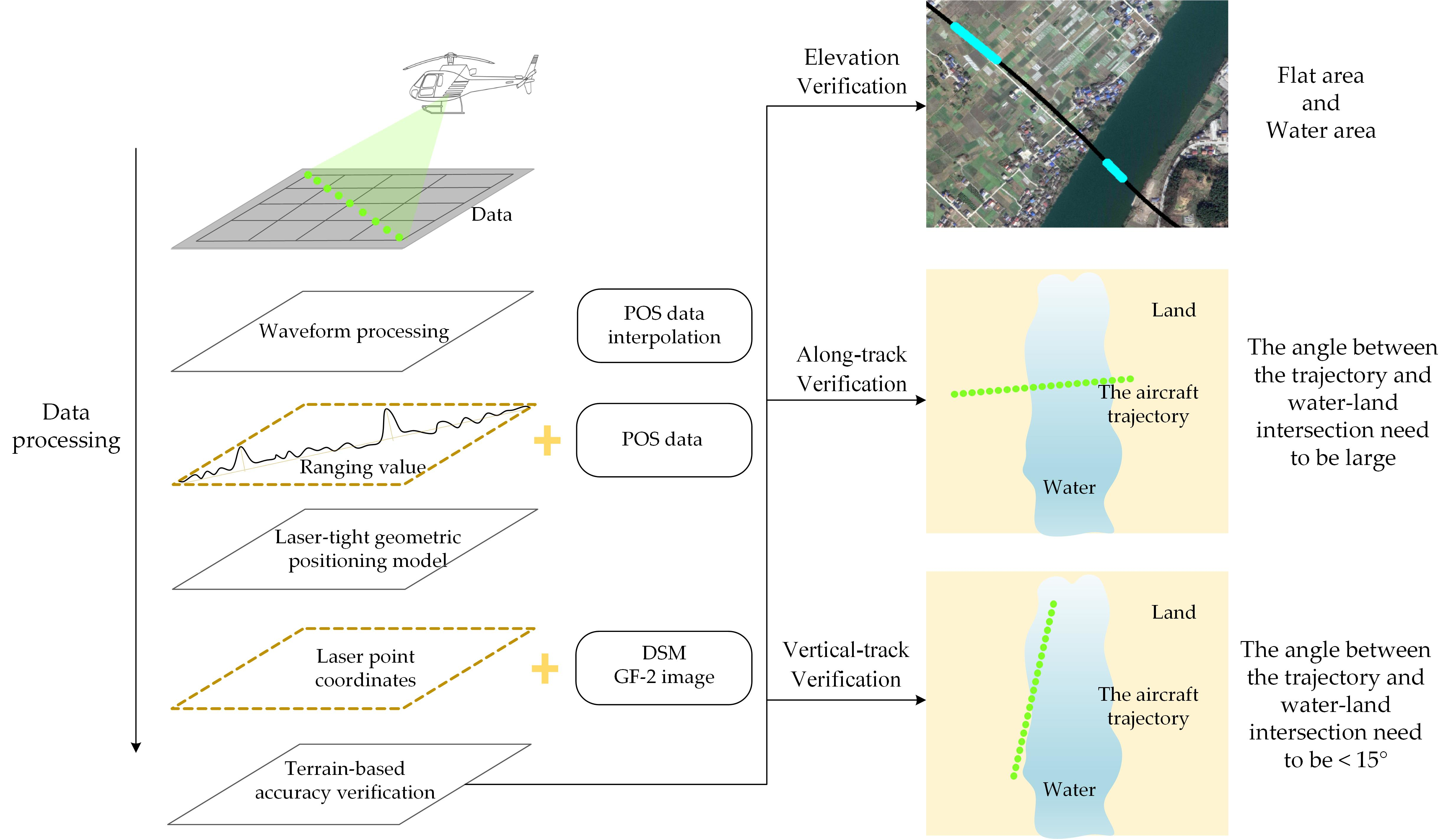
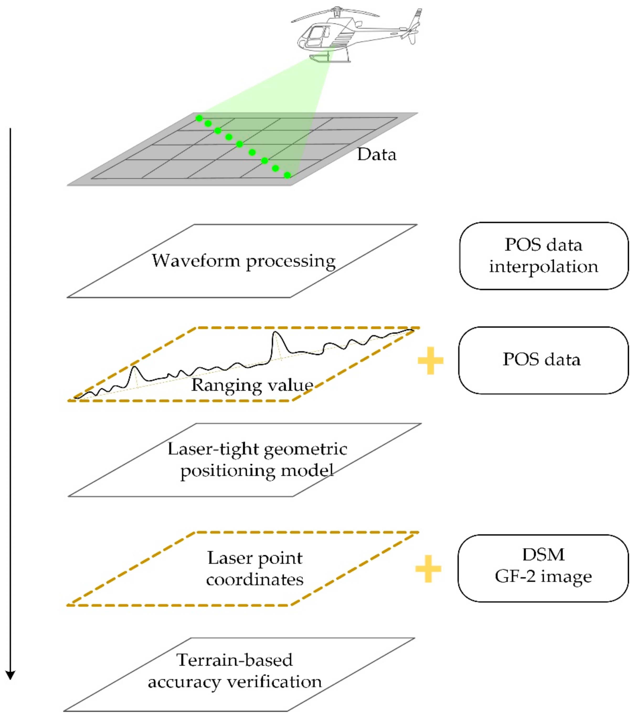
2.2. Data Processing
The workflow of our proposed method can be summarized as follows (Figure 2):
- Waveform data reading: The large-footprint lidar data and POS data are read. POS data are interpolated for consistency with the lidar waveform time.
- Waveform pre-treatment: The lidar data are pre-processed, including data interpretation and removal of waveform noise, in order to reduce the influence of noise on the positioning accuracy.
- Main peak extraction: To deal with echo signal saturation, the COG method is used to define the peaks of the incident wave and echo and relocate the main peak, allowing the distance between the laser and the measured object to be calculated according to the time of the incident wave and echo wave peak.
- Geometrical positioning: The laser-tight geometric positioning model is used to calculate the three-dimensional laser point coordinates by combining the ranging value and POS data.
- Accuracy verification: The terrain features are used to verify the elevation and plane accuracy of airborne lidar data.
2.2.1. Signal Saturation Processing
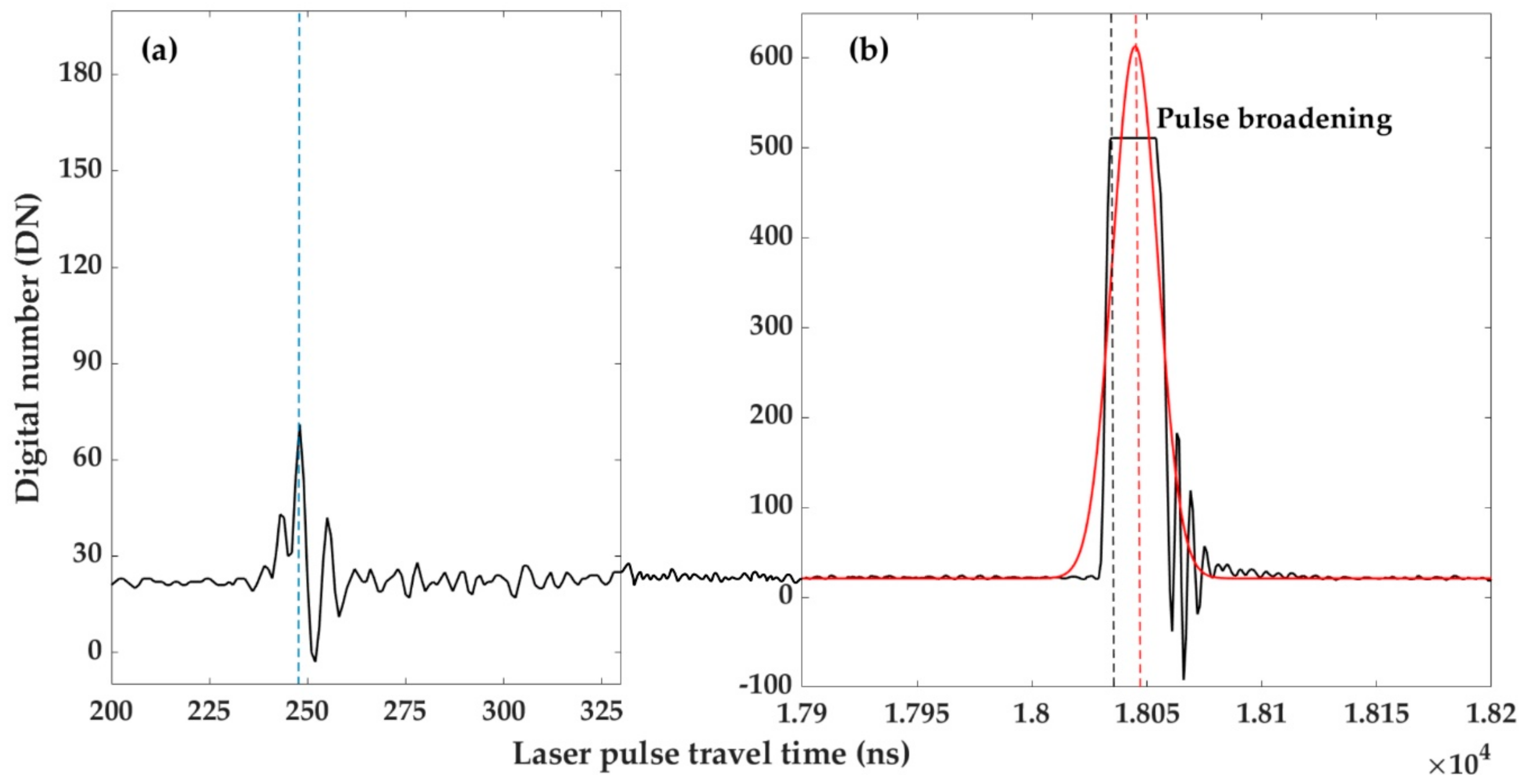
Airborne large-footprint lidar systems are predominantly composed of a laser, telescope, relay optical system, detector, and signal acquisition and processing subsystem [29]. All signal amplifiers in lidar detector electronic circuits have finite linear dynamic ranges [24]. When the weather is clear and the surface reflectance is high (e.g., a calm water surface), the peak power of the echo pulse will exceed the linear dynamic range of the receiver, resulting in signal saturation, and the echo waveforms will exhibit peak clipping and pulse broadening [12,30,31] (Figure 3). Laser ranging uses the time difference between pulse transmission and reception to calculate the distance:
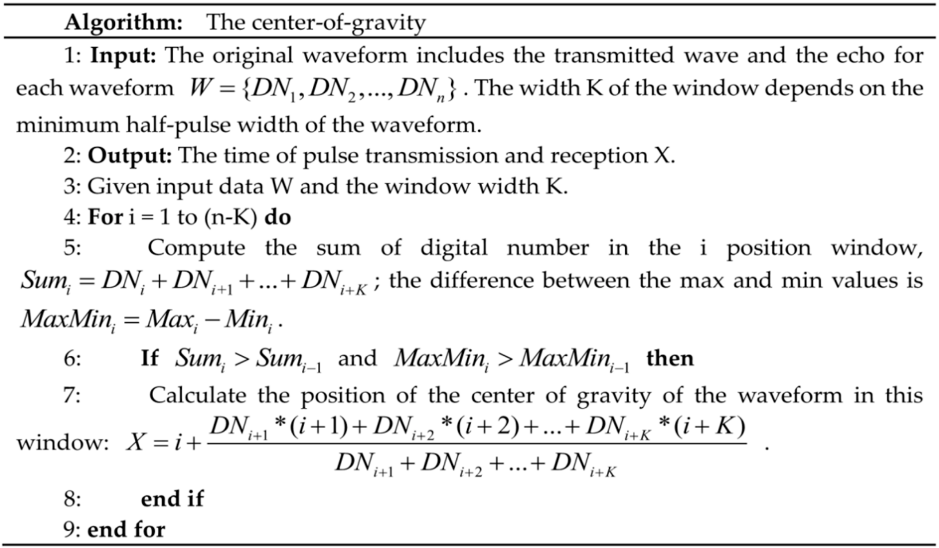
where ρ is the distance, c is the speed of light, TRecieve is the pulse reception time, and TEmission is the pulse transmission time. Such pulse broadening will increase the travel time of the laser pulse. A traditional approach uses Gaussian fitting of the echo centroids to determine the arrival time [32]. However, the above method directly affects the ranging when the pulse is saturated, making the measured surface elevation lower than the actual one. Since our proposed method relied on the accuracy of the water surface elevation, we proposed the COG method to determine the arrival time. When the pulse is saturated, the leading edge of the delay is taken as the position of the main peak, and the time of pulse transmission and reception is calculated according to the change in the waveform energy value in the region where the main peak is located (Figure 4).
2.2.2. Laser-Tight Geometric Positioning Model
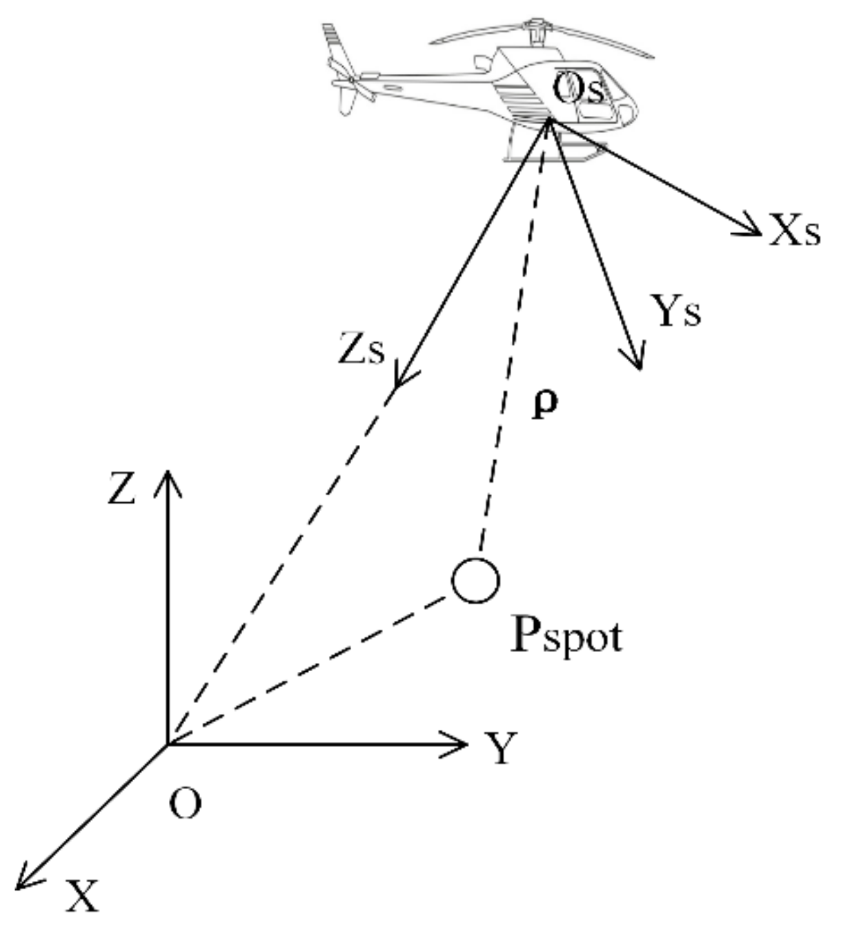
We constructed a laser-tight geometric positioning model based on the principles of lidar altimetry [33,34,35]. Assuming that the Earth’s inertial coordinate system (O-XYZ) is known, the aircraft’s body coordinate system (Os – XsYsZs) can be defined by using the centroid of the aircraft as the origin, the Zs-axis pointing in the geocentric direction, the Xs-axis pointing in the flight direction, and the Ys-axis following the right-hand rule (Figure 5).
The laser-tight geometric positioning model is calculated as follows:
where is the coordinate of the laser footprint in the World Geodetic System 1984 (WGS84) [36], is the position coordinate measured by the aircraft’s GPS at the time of pulse emission, is the speed of laser propagation in a vacuum, is the time transfer by laser pulses, is the compensation amount for the laser ranging time, and is the rotation matrix from the East, North, and Up (ENU) coordinate system to the WGS84 coordinate system. The local ENU coordinate system can be defined by placing the origin in the earth-fixed local point, while the X-axis points in the eastward direction (E), the Y-axis points in the northward direction (N), and the Z-axis is in the same orientation as the vertical (U) [37]. is the rotation matrix from the body coordinate system to the ENU coordinate system, and is the set over matrix related to the laser beam exit angle [22,35].
2.3. Accuracy Verification Method
2.3.1. Verification of Elevation Accuracy
It is necessary to select a simple flat surface, such as bare level land, when verifying the elevation accuracy. Such terrain may not exist in practice; however, the elevation change of a calm water surface is negligible so can be used instead. In shallow water areas, echoes from plants and the water bottom can affect the elevation accuracy, so a location in the center of a wider water area should be selected. The processed elevation value of each laser point can then be compared with the actual elevation value recorded by a DSM, allowing the removal of approximate values, calculation of the mean error and the root mean square error, and assessment of the elevation error. Moreover, the acquisition time of the high-precision DSM used for comparison should be similar to the experimental data.
2.3.2. Verification of Positioning Accuracy Along the Orbital Direction
When there is a distinct elevation difference between an area’s features, such as the intersection between water and land or that between buildings and land, the positioning accuracy can be verified by tracing back the change in echo waveform across the relevant footprint. Due to better recognition of the water–land intersection in high-resolution imagery and different echo characteristics between the water and land, we chose these terrain features to verify the plane accuracy. When the aircraft trajectory is perpendicular to the water–land intersection, or the angle between the trajectory and the water–land intersection is large, it is possible to retrace the laser point path across this terrain. The changes in peak shape and echo waveform position can then be used to define the water and land footprints in order to verify the plane accuracy in the orbital direction (Figure 6 and Figure 7).
In this situation, the method comprises the following steps:
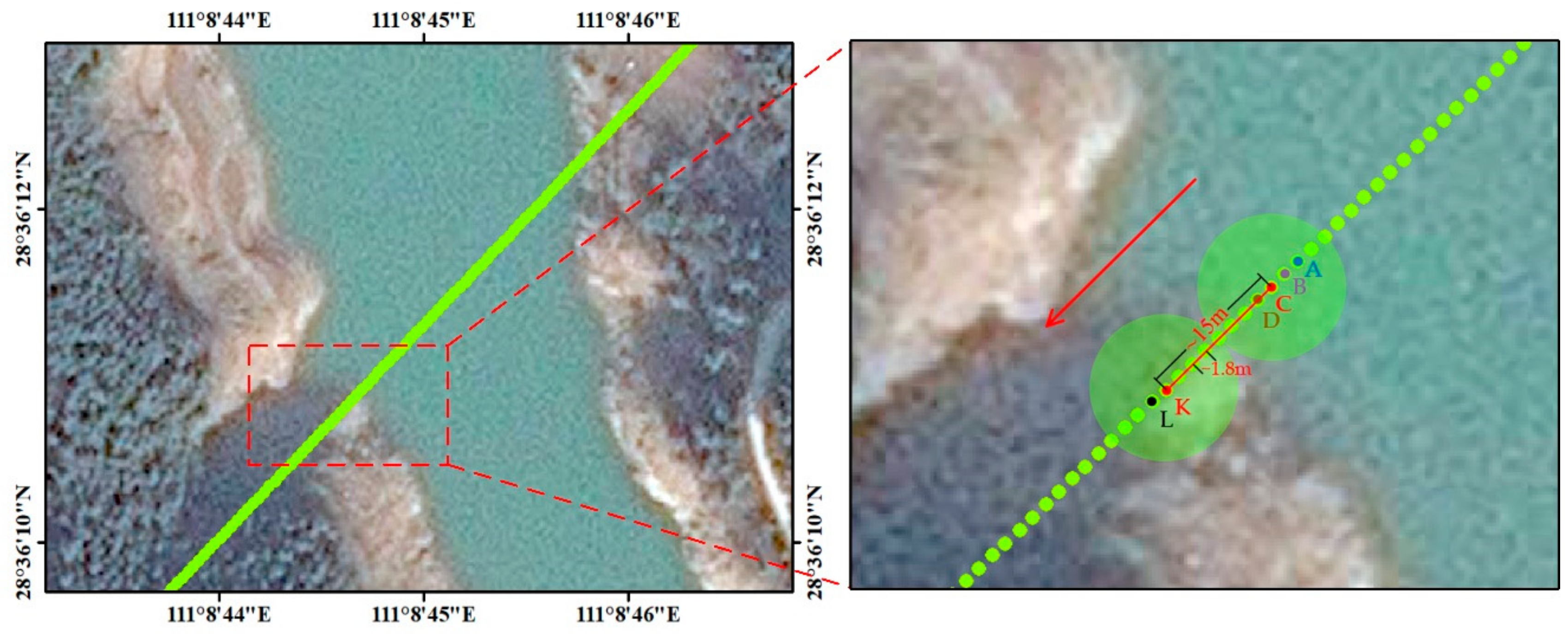
- Footprint selection: The laser spot location map is combined with the high-resolution remote sensing image, which enables an appropriate laser spot A on the water surface to be found through visual interpretation (Figure 6).
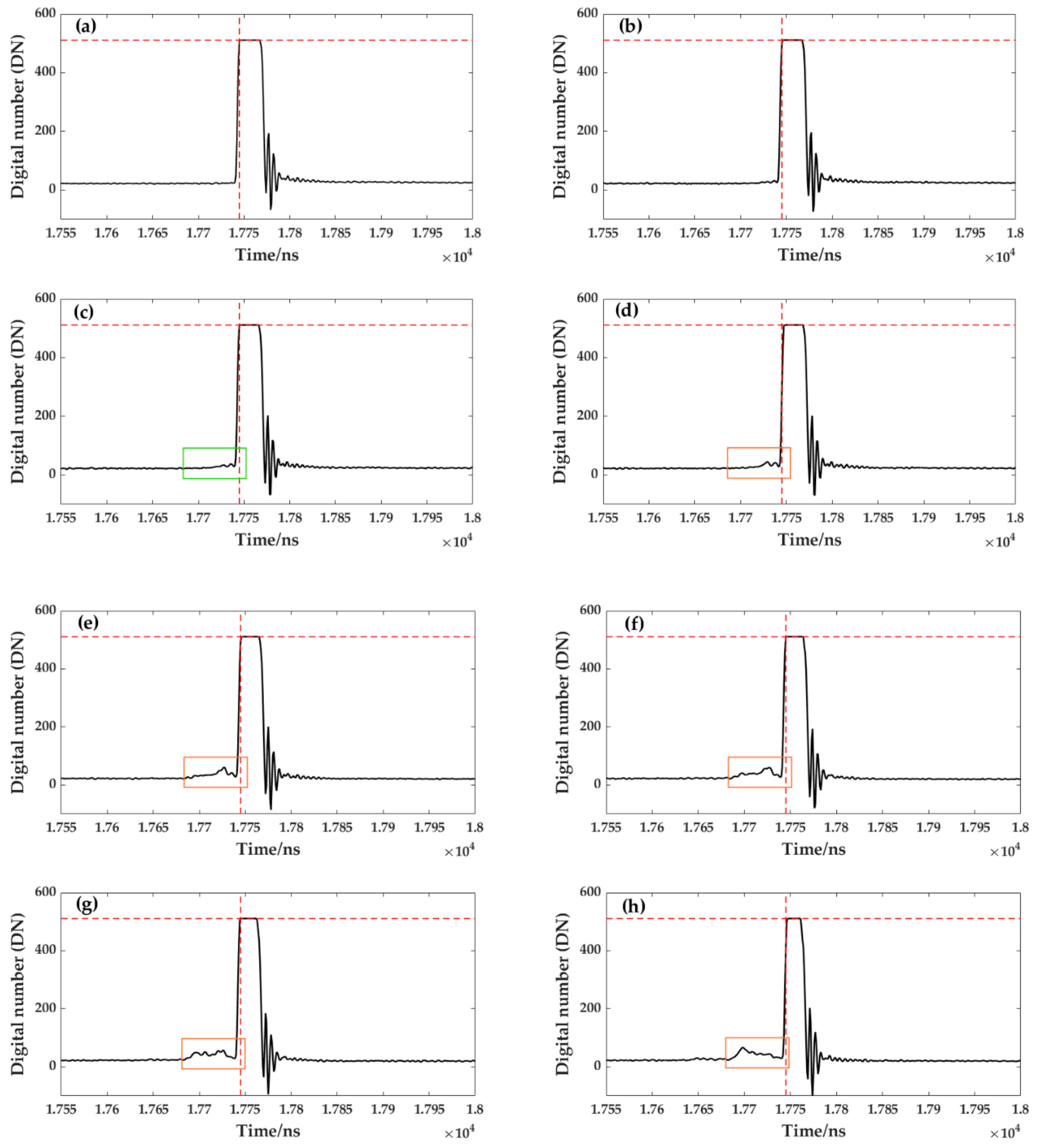
- Waveform search: The echo waveform corresponding to the selected spot A is assessed. Due to the high reflection intensity at the calm water surface, the echo signal corresponding to spot A is continuously saturated (Figure 7a). Marking the starting position of the spot saturation denotes the echo peak position of the water surface (red dotted line in Figure 7).
- Process backtracking: The corresponding waveform of each spot from the position of spot A is viewed in the landward direction. Figure 7 shows the echo waveform corresponding to each spot from A to I in Figure 6. When the feature covered by the footprint begins to appear on the land, the echo waveform will have two echoes, one from the water surface and the other from the land surface. Because the elevation of the land is higher than that of the water surface, the echo waveform on the land will appear in front of that from the water surface, according to the echo time (orange rectangle in Figure 7). When continuing to view the waveform of the laser spot in the landward direction, the saturation of the water spot weakens, as does the echo intensity until it disappears. Meanwhile, the amplitude of the land echo signal is gradually increasing.
- Footprint judgment: By observing the appearance of the land echo signal and the disappearance of the water echo signal, it is possible to judge that the footprint before the appearance of the land echo waveform is the last laser footprint that completely falls in the water surface; this can be defined as the footprint of the water surface. Similarly, when the wave peak at the water surface disappears completely, this footprint can be defined as the footprint of the land. However, due to the influence of noise or tree branches, it is not easy to determine the footprint where the land echo waveform begins to appear and where the water echo waveform completely disappears. For instance, the waveform before the echo peak position of the water surface of spot C is not obvious (green rectangle in Figure 7c), and it is not possible to determine whether this is a land echo or noise. Similarly, it is not easy to determine whether there is a water echo at the echo peak position of the water of spot K (blue rectangle in Figure 7k). Therefore, we combine the footprint spot diameter to assist the judgment. Because the footprint spot diameter is ~15 m, we require the center distance between the water and land footprints to be approximately 15 m when judging the two spots, which also ensures that the footprints of water and land are tangent. The spacing of the laser spots is ~1.8 m, spot C and spot K are separated by eight spaces, about 15 m. Therefore, we judge that the insignificant echo is noise and defined spot C as the footprint of the water surface and spot K as the footprint of the land surface.
- Error calculation: Because the footprints of water and land are tangent, the halfway point of the central line between the water and land footprint spots can be taken as the measured intersection position (Figure 6). Then, by finding the actual position of the boundary between the water and land surfaces using DSM data, the lidar positioning error along the track can be determined.
2.3.3. Verification of the Positioning Accuracy Perpendicular to the Orbital Direction
Verification of the plane accuracy includes verification along the orbital direction and vertical orbital direction. When there is a small angle between the trajectory and the water–land intersection, due to the existence of the vertical orbital error, the waveform of the footprint spot falling on the land may be saturated or vice versa. Accounting for this allows the plane accuracy perpendicular to the orbital direction to be verified (Figure 8).
In this situation, the method comprises the following steps:
- Area selection: First, the laser spot location map is combined with the high-resolution remote sensing image, and trajectories with angles of < 15° with the water–land intersection are determined by visual interpretation (Figure 8).
- Waveform comparison: The waveform corresponding to the land footprint intersection with the trajectory is located. If the waveform diagram of the land is saturated, this means that the footprint spot has shifted to the land in the vertical orbit direction. Similarly, if the wave pattern corresponding to the footprint spot in the water is not saturated, this means that the footprint spot is offset toward the water in the vertical direction.
- Actual positioning: There is a certain elevation difference between water and land. Following the direction of the vertical track of the shifted spot, the location of the spot’s elevation can be determined through the elevation change of the DSM; this is the actual position.
- Error calculation: The difference between the offset spots on the route track and the actual position is determined, and the average error value is recorded as the vertical orbit positioning error.
3. Results
Using the proposed accuracy verification method for airborne large-footprint lidar based on terrain features (Section 2.3), the elevation and plane accuracy of the data processed by the processing flow shown in Figure 2 are verified.
3.1. Verification of Laser Elevation Accuracy
3.1.1. Flat Areas
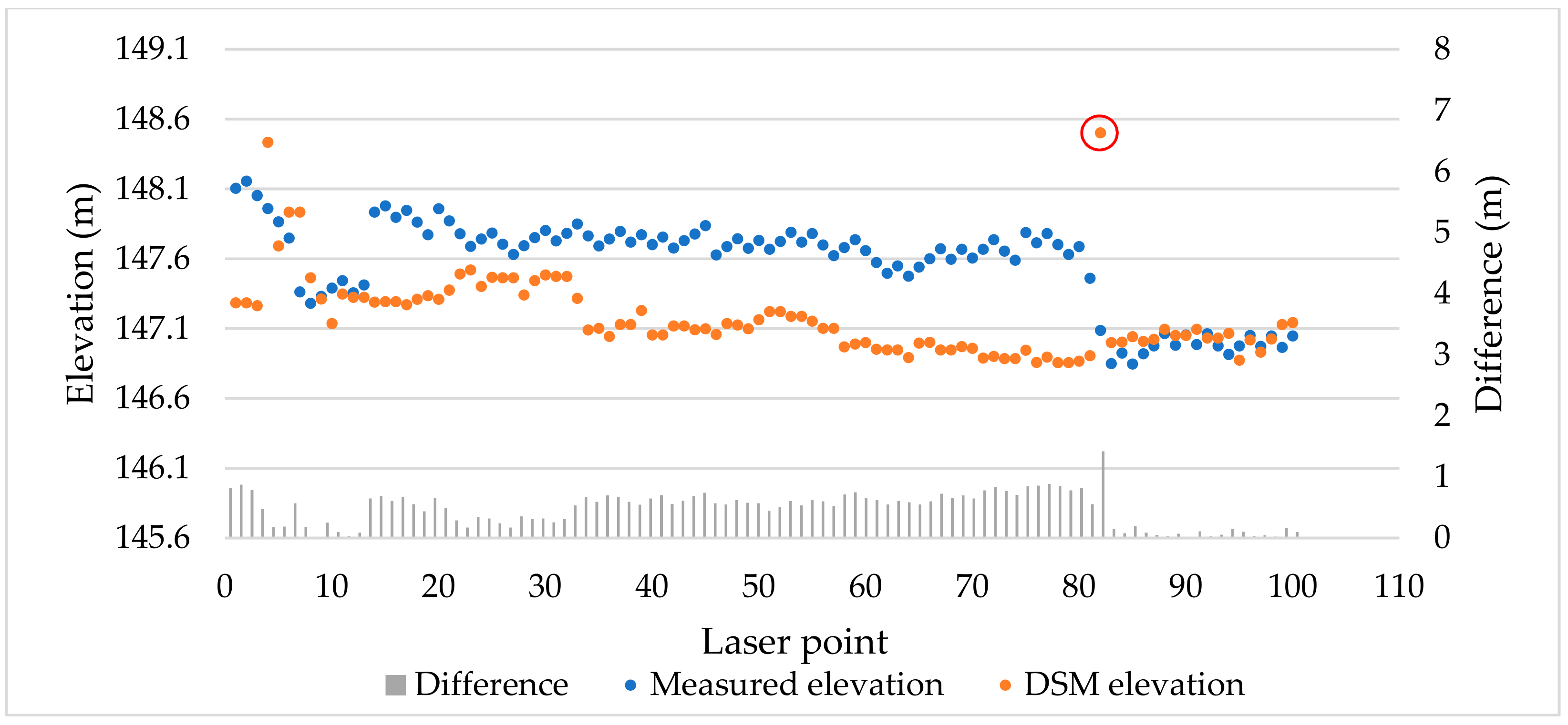
We considered wintertime unplanted farmland as an appropriate proxy for the bare flat land required by our method (Figure 9). One hundred groups of laser data were selected on this type of ground in Area 1 to verify the elevation accuracy using DSM data. The processing elevation of each laser point was then compared with the actual elevation of DSM (Figure 10). The mean error was 0.39 m and the root mean square error (RMSE) was 0.55 m. One point had a difference of > 1 m (red circle in Figure 10). There was a sudden change in the DSM value at this point, perhaps caused by a temporary ground object during DSM measurement.
3.1.2. Water Areas
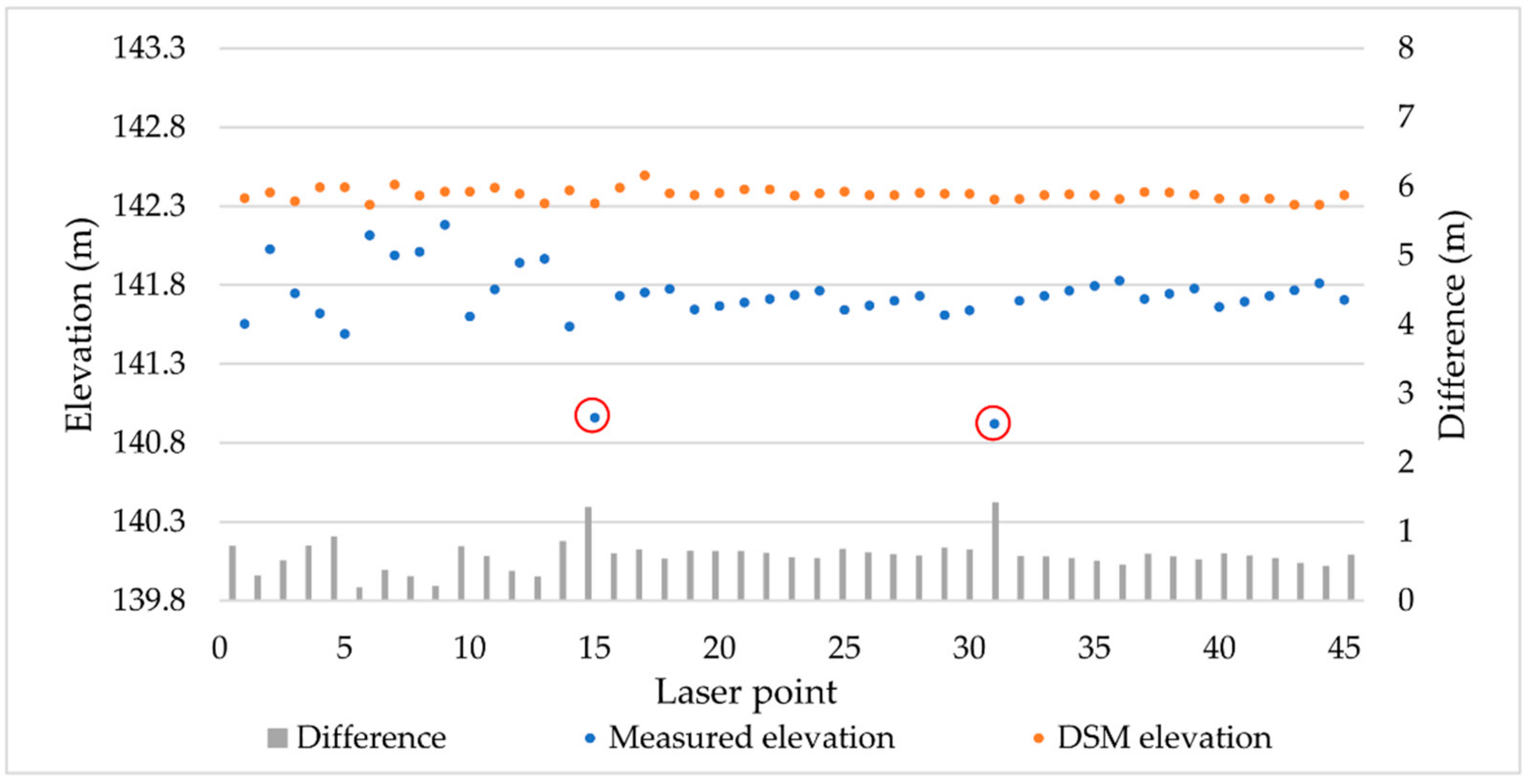
We selected 45 groups of laser data, centered within wider water areas, to verify the water surface elevation accuracy by comparing the measured and DSM elevation values (Figure 11). Two points had differences of > 1 m (red circles in Figure 11). A comparison with the original transmitted wave reveals that these errors were caused by abnormal triggering of the laser. Overall, the mean error for water surface elevation was 0.65 m and the RMSE was 0.69 m. The echo waveforms of the flat and water were simple, which avoids the influence of ground features on elevation accuracy. The RMSE of the flat area was 0.55 m and the RMSE of the water area was 0.69 m, both of which are less than 1 m. These results show that the laser elevation data is reliable.
3.1.3. Effect of the COG Method
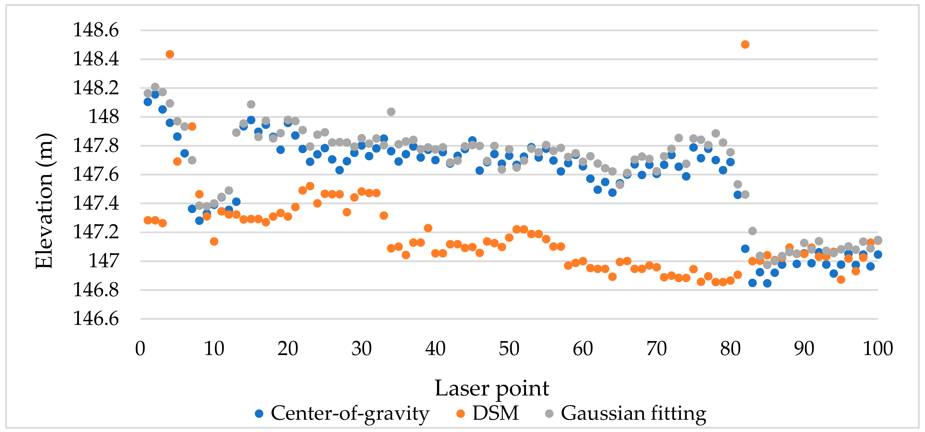
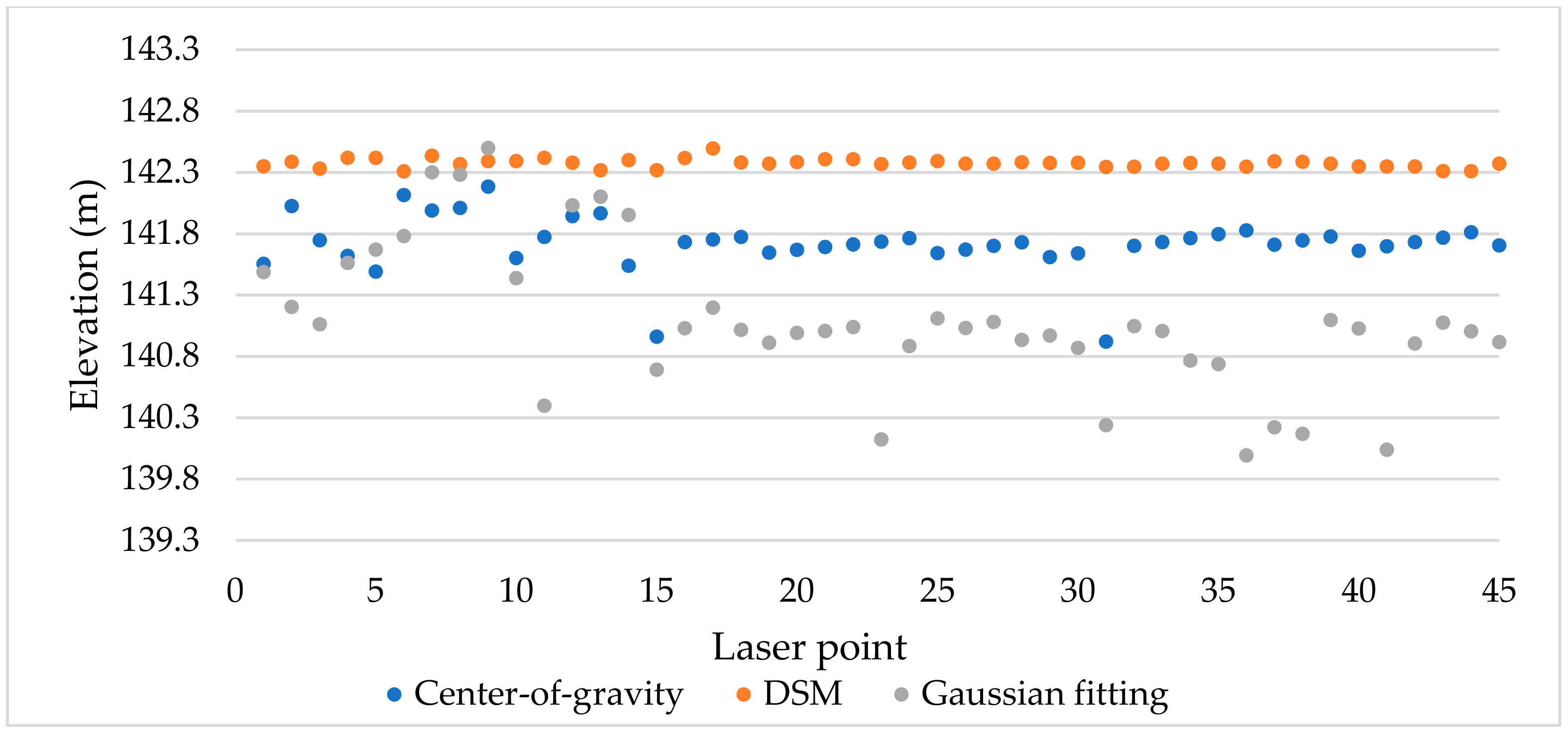
In our data processing, we presented the COG method for resolving the saturation problem. To verify the effectiveness of this method, we compared the validation results of the elevation accuracy of the Gaussian fitting method with the COG method (Table 2). As expected, the COG method outperformed the Gaussian fitting method in terms of the mean error and RMSE values. In flat areas, the results of the two methods do not differ much (Figure 12). However, for water areas, the COG method can obviously improve the phenomenon of low measured values caused by the traditional Gaussian fitting method (Figure 13), which indicates that the method proposed in this study can well deal with the saturation problem and improve the measurement accuracy.
3.2. Verification of Laser Plane Accuracy
3.2.1. Along-track Verification
In three areas of plane accuracy verification (Areas 2–4), where the trajectory of the route was perpendicular to the water surface, six groups were selected in each, resulting in a total of 18 groups of data. These were used to verify the positioning accuracy along the orbit in terms of the mean error values (Table 3).
The average mean positioning error along the orbit direction was 3.25 m, which meets our required limit of 5 m. There was no significant difference between the three measurement areas. In this direction, the measured values were offset ahead of the DSM values in the flight direction; however, the deviation values were different, showing that flight speed impacts the accuracy. However, because the aircraft flight was not smooth and the speed was not consistent, this offset was not stable. These results show that our method for determining the positional error of the laser along the orbital direction based on terrain features can be used to test the along-track positioning accuracy of large-footprint lidar, as long as errors caused by human factors and complex interior objects in the footprint can be avoided.
3.2.2. Vertical Track Plane Positioning Accuracy
For special terrains where the angle between the trajectory and shoreline was < 15° in the three measured areas, the offset of five laser footprint spots were taken in each special terrain and averaged. As the method requires a lower angle between the trajectory and water–land intersection, only five feasible locations could be selected for this verification (Table 4). The positioning errors were similar for all five tracks; the average of 4.17 m meets our requirement of 5 m. All tracks were shifted to the left-hand side of the flight direction, showing that the aircraft attitude influenced the vertical orbit positioning of the laser points. However, due to the limited verification data, the size of this systemic difference could not be accurately expressed. These limited results suggest that this method can verify the vertical orbit positioning accuracy when the terrain and footprint waveforms meet the requirements of the proposed method.
4. Discussion
4.1. Data Processing Analysis
For the data processing, the complete process was constructed from the original data to the positioning data and the saturation was processed, in contrast to other methods. In the airborne experiment, the data acquisition time was short, the measurement range was small, and the aircraft altitude was low; thus, the effects of atmosphere and tides are ignored during processing. For spaceborne experiments, it is necessary to correct for the atmosphere and tide. Then, because only simple terrain was processed in this verification, no wave decomposition was performed. In order to analyze complex features, inverse feature information, etc., waveform decomposition should be added to this method.
4.2. Evaluation of Accuracy Verification Method
4.2.1. Applicability Analysis
Our method has specific requirements for terrain and aircraft trajectory as it requires either the trajectory of the route to be perpendicular to the water surface or the angle between the trajectory and the water–land intersection to be large when verifying the along-track accuracy. Moreover, when verifying the vertical-track accuracy, it requires the angle between the trajectory and water–land intersection to be < 15°. As such, this method is not applicable in regions with insufficient water; thus, other verification methods can be used in these cases, for example waveform matching. In our experiment, due to the hardware, the transmission pulse width is too narrow to record all the pulses in a nanosecond, which caused the recorded transmitted wave signal to fail to reflect the true energy distribution. Therefore, the simulation waveform does not match the real waveform, which makes it impossible to use the waveform matching method for verification experiments.
4.2.2. Error Analysis
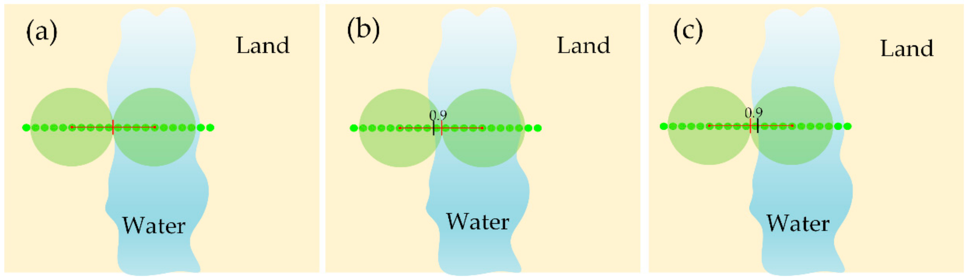
In our method, when verifying the plane accuracy, we take the halfway point of the central line between the water and land footprint spots as the measured intersection position. Ideally, the center of the line connecting the two footprint spots is exactly at the intersection (Figure 14a). In practice, the central location will be some distance from the water–land intersection. Here, we analyzed the situation with the largest deviation (Figure 14b–c). Because the footprint spot spacing is ~1.8 m, when the distance between the footprint spot and the intersection is greater than 0.9 m, there must be another adjacent footprint spot with a distance less than 0.9 m from the intersection. In this case, another spot can be used, so the maximum deviation distance between the central location and the water–land intersection is 0.9 m.
When verifying the plane accuracy, subjective judgments regarding water–land intersections and waveforms can produce errors. Due to the influence of noise or tree branches, the location of the water footprint spot and the land spot cannot be easily determined by only analyzing the waveforms. Therefore, we combine the footprint spot diameter to ensure that the distance between the centers of the two spots is ~15 m. This not only ensures that the two footprint spots are tangent, but also can eliminate some subjective judgment errors. Determining the water–land intersection through the DSM and remote sensing images can also produce pixel errors of 1–2; therefore, it is necessary to select a high-resolution image and determine the position of the intersection by analyzing the elevation change using the DSM to reduce subjective judgment errors.
5. Conclusions
In this paper, factors such as surface contour and surface reflectance are considered comprehensively, and the topographic features of the experimental area are fully utilized. We proposed a flexible and efficient accuracy verification method for airborne large-footprint lidar based on terrain features, which not only guarantees the accuracy of elevation but also the accuracy of the plane position. Our method utilizes the terrain features for verification, which reduces the manpower and material resources required for the laser detector. Moreover, we developed a new processing method that improves data quality by targeting the pulse broadening caused by signal saturation over water. Our experimental trials verified that the elevation and plane positioning accuracy meet the design requirements in all directions. Our method confirms the performance of a new instrument and guarantees the applicability of the data. However, as this method has certain limitations imposed by the terrain and other factors, further research is required to resolve these issues.
Author Contributions
Conceptualization, W.L., S.L., G.Z. and X.C.; Funding acquisition, S.L. and G.Z.; Methodology, W.L., S.L. and X.C.; Software, W.L., S.L. and X.C.; Writing—original draft, W.L.; Writing—review & editing, W.L., S.L., G.Z., Y.W., X.C. and H.C. All authors have read and agreed to the published version of the manuscript.
Funding
This research was supported by the National Natural Science Foundation of China (Grant No. 41901400), the China Postdoctoral Science Foundation (2018M632919), and the National High Resolution Earth Observation Foundation (11-Y20A12-9001-17/18).
Acknowledgments
We thank China’s State Forestry Administration for providing the lidar data. We also thank the anonymous reviewers for their constructive feedback.
Conflicts of Interest
The authors declare no conflict of interest.
References
- Wang, C.; Menenti, M.; Stoll, M.P.; Li, C.; Tang, L. Error analysis & correction of airborne LiDAR data (in Chinese). J. Remote Sens. 2007, 3, 390–397. [Google Scholar]
- Tian, J.; Wang, L.; Li, X.; Yin, D.; Gong, H.; Nie, S.; Shi, C.; Zhong, R.; Liu, X.; Xu, R. Canopy Height Layering Biomass Estimation Model (CHL-BEM) with Full-Waveform LiDAR. Remote Sens. 2019, 11, 1446. [Google Scholar] [CrossRef] [Green Version]
- Fayad, I.; Baghdadi, N.; Bailly, J.-S.; Barbier, N.; Gond, V.; Hajj, M.E.; Fabre, F.; Bourgine, B. Canopy Height Estimation in French Guiana with LiDAR ICESat/GLAS Data Using Principal Component Analysis and Random Forest Regressions. Remote Sens. 2014, 6, 11883–11914. [Google Scholar] [CrossRef] [Green Version]
- Ali, S.A.; Sridhar, V. Deriving the Reservoir Conditions for Better Water Resource Management Using Satellite-Based Earth Observations in the Lower Mekong River Basin. Remote Sens. 2019, 11, 2872. [Google Scholar] [CrossRef] [Green Version]
- Chipman, J.W. A Multisensor Approach to Satellite Monitoring of Trends in Lake Area, Water Level, and Volume. Remote Sens. 2019, 11, 158. [Google Scholar] [CrossRef] [Green Version]
- Ferreira, L.G.; Urban, T.J.; Neuenschawander, A.; De Araújo, F.M. Use of Orbital LIDAR in the Brazilian Cerrado Biome: Potential Applications and Data Availability. Remote Sens. 2011, 3, 2187–2206. [Google Scholar] [CrossRef] [Green Version]
- Blair, J.B.; Rabine, D.L.; Hofton, M.A. The Laser Vegetation Imaging Sensor: A medium-altitude, digitization-only, airborne laser altimeter for mapping vegetation and topography. ISPRS J. Photogramm. Remote Sens. 1999, 54, 115–122. [Google Scholar] [CrossRef]
- Park, T.; Kennedy, R.E.; Choi, S.; Wu, J.; Lefsky, M.A.; Bi, J.; Mantooth, J.A.; Myneni, R.B.; Knyazikhin, Y. Application of Physically-Based Slope Correction for Maximum Forest Canopy Height Estimation Using Waveform Lidar across Different Footprint Sizes and Locations: Tests on LVIS and GLAS. Remote Sens. 2014, 6, 6566–6586. [Google Scholar] [CrossRef] [Green Version]
- Jansma, P.; Mattioli, G.; Matias, A. Slicer laser altimetry in the eastern Caribbean. Surv. Geophys. 2001, 22, 561–579. [Google Scholar] [CrossRef]
- Schutz, B.E.; Zwally, H.J.; Shuman, C.A.; Hancock, D.; DiMarzio, J.P. Overview of the ICESat mission. Geophys. Res. Lett. 2005, 32, L21S01. [Google Scholar] [CrossRef] [Green Version]
- Peterson, B.; Nelson, K.J. Mapping Forest Height in Alaska Using GLAS, Landsat Composites, and Airborne LiDAR. Remote Sens. 2014, 6, 12409–12426. [Google Scholar] [CrossRef] [Green Version]
- Fricker, H.A.; Borsa, A.; Minster, B.; Carabajal, C.; Bills, B. Assessment of ICESat performance at the Salar de Uyuni, Bolivia. Geophys. Res. Lett. 2005, 32, L21S06. [Google Scholar] [CrossRef] [Green Version]
- Smith, D.E.; Zuber, M.T.; Neumann, G.A.; Lemoine, F.G.; Mazarico, E.; Torrence, M.H.; McGarry, J.F.; Rowlands, D.D.; Head, J.W.; Duxbury, T.H.; et al. Initial observations from the Lunar Orbiter Laser Altimeter (LOLA). Geophys. Res. Lett. 2010, 37, L18204. [Google Scholar] [CrossRef]
- Li, G.; Tang, X. Analysis and validation of ZY-3 02 satellite laser altimetry data. Acta Geod. Et Cartogr. Sin. 2017, 46, 1939–1949. [Google Scholar] [CrossRef]
- Tang, X.; Xie, J.; Liu, R.; Huang, G.; Zhao, C.; Zhen, Y.; Tang, H.; Dou, X. Overview of the GF-7 laser altimeter system mission. Earth Space Sci. 2019, 7, 1–11. [Google Scholar] [CrossRef]
- Magruder, L.; Silverberg, E.; Webb, C.; Schutz, B. In situ timing and pointing verification of the ICESat altimeter using a ground-based system. Geophys. Res. Lett. 2005, 32, L21S04. [Google Scholar] [CrossRef] [Green Version]
- Magruder, L.A.; Suleman, M.A.; Schutz, B.E. ICESat laser altimeter measurement time validation system. Meas. Sci. Technol. 2003, 14, 1978–1985. [Google Scholar] [CrossRef] [Green Version]
- Magruder, L.A.; Ricklefs, R.L.; Silverberg, E.C.; Horstman, M.F.; Suleman, M.A.; Schutz, B.E. ICESat geolocation validation using airborne photography. IEEE Trans. Geosci. Remote Sens. 2010, 48, 2758–2766. [Google Scholar] [CrossRef]
- Schutz, B.E. Calibration/Validation of ICESat laser altimeter (GLAS). In Proceedings of the American Geophysical Union, Spring Meeting 2002, Washington, DC, USA, 30 May 2002. [Google Scholar]
- Magruder, L.A.; Schutz, B.E.; Silverberg, E.C. Laser pointing angle and time of measurement verification of the ICESat laser altimeter using a ground-based electrooptical detection system. J. Geod. 2003, 77, 148–154. [Google Scholar] [CrossRef]
- Magruder, L.A.; Webb, C.E.; Urban, T.J.; Silverberg, E.C.; Schutz, B.E. ICESat altimetry data product verification at White Sands Space Harbor. IEEE Trans. Geosci. Remote Sens. 2007, 45, 147–155. [Google Scholar] [CrossRef]
- Zhang, G.; Li, S.; Huang, W. Geometric calibration and validation of ZY3-02 satellite laser altimeter System. Geomat. Inf. Sci. Wuhan Univ. 2017, 11, 92–99. [Google Scholar]
- Tang, X.; Xie, J.; Fu, X.; Mo, F.; Li, S.; Dou, X. ZY3-02 laser altimeter on-orbit geometrical calibration and test. Acta Geod. Et Cartogr. Sin. 2017, 46, 714–723. [Google Scholar] [CrossRef]
- Martin, C.F.; Thomas, R.H.; Krabill, W.B.; Manizade, S.S. ICESat range and mounting bias estimation over precisely-surveyed terrain. Geophys. Res. Lett. 2005, 32, 242–257. [Google Scholar] [CrossRef] [Green Version]
- Harding, D.J. ICESat waveform measurements of within-footprint topographic relief and vegetation vertical structure[J]. Geophys. Res. Lett. 2005, 32, L21S10. [Google Scholar] [CrossRef] [Green Version]
- Sun, X.; Abshire, J.B.; Borsa, A.A.; Fricker, H.A.; Yi, D.; DiMarzio, J.P.; Paolo, F.S.; Brunt, K.M.; Harding, D.J.; Neumann, G.A. ICESAT/GLAS altimetry measurements: Received signal dynamic range and saturation correction. IEEE Trans. Geosci. Remote Sens. 2017, 55, 5440–5454. [Google Scholar] [CrossRef]
- Wu, F.; Gao, X.; Pan, C. Design and application of forest detecting based on airborne large-footprint LiDAR system. For. Res. Manag. 2018, 125–132. [Google Scholar] [CrossRef]
- Chen, X. Waveform processing and accuracy verification of airborne large-footprint LiDAR system. Master’s Thesis, Wuhan University, Wuhan, China, 2019. [Google Scholar]
- Zhou, H.; Chen, Y.; Hyyppa, J.; Li, S. An overview of the laser ranging method of space laser altimeter. Infr. Phys. Technol. 2017, 86, 147–158. [Google Scholar] [CrossRef]
- Abshire, J.B.; Sun, X.; Riris, H.; Sirota, J.M.; McGarry, J.F.; Palm, S.; Yi, D.; Liiva, P. Geoscience laser altimeter system (GLAS) on the ICESat mission: On-orbit measurement performance. Geophys. Res. Lett. 2005, 32, 2–21. [Google Scholar] [CrossRef] [Green Version]
- ICESat/GLAS Data: Description of Past Data Releases. National Snow and Ice Data Center. Available online: http://nsidc.org/data/icesat/past_releases.html (accessed on 15 December 2019).
- Brenner, A.C.; Zwally, H.J. The algorithm theoretical basis document for the derivation of range and range distributions from laser pulse waveform analysis for surface elevations, roughness, slope, and vegetation heights. Available online: https://nsidc.org/data/icesat/technical-references (accessed on 15 December 2019).
- Li, G. Earth observing satellite laser altimeter data processing method and engineer practice. Ph.D. Thesis, Wuhan University, Wuhan, China, 2017. [Google Scholar]
- Tang, X.; Li, G.; Gao, X.; Chen, J. The rigorous geometric model of satellite laser altimeter and preliminarily accuracy validation. Acta Geod. Et Cartogr. Sin. 2016, 45, 1182–1191. [Google Scholar] [CrossRef]
- Li, S. Research on geometric calibration of Earth observation satellite laser altimeter. Ph.D. Thesis, Wuhan University, Wuhan, China, 2017. [Google Scholar]
- Hassan, A.; Mustafa, E.K.; Mahama, Y.; Damos, M.A.; Jiang, Z.; Zhang, L. Analytical Study of 3D Transformation Parameters Between WGS84 and Adindan Datum Systems in Sudan. Arab J Sci Eng 2020, 45, 351–365. [Google Scholar] [CrossRef]
- Wand, D.; Pang, B.; Xiao, W. GEO space debris flux determination based on earth-fixed coordinate system. Acta Astronaut. 2017, 130, 60–66. [Google Scholar] [CrossRef]
Figure 1.
Map of airborne large-footprint lidar measurement areas used in this study. Area 1 was used to verify the elevation accuracy, whereas Areas 2–4 were used to verify the plane accuracy.
Figure 1.
Map of airborne large-footprint lidar measurement areas used in this study. Area 1 was used to verify the elevation accuracy, whereas Areas 2–4 were used to verify the plane accuracy.

Figure 2.
Flow chart of the proposed lidar data processing method.

Figure 3.
Schematic diagram of the echo wave pattern at signal saturation for (a) the transmitted pulse and (b) the received pulse. The solid red line is a Gaussian-fitted waveform, the dotted red line is the time of pulse reception obtained by the Gaussian fitting method, the solid black line is a broadened pulse resulting from signal saturation, and the time corresponding to the dotted black line is the pulse reception time obtained by the center-of-gravity (COG) method.

Figure 4.
The COG method.

Figure 5.
Schematic diagram of the laser-tight geometric positioning model.

Figure 6.
Schematic of laser spot locations at the intersection between water and land. The red arrow indicates the landward direction.
Figure 6.
Schematic of laser spot locations at the intersection between water and land. The red arrow indicates the landward direction.

Figure 7.
(a–l) are echo waveform diagrams corresponding to each spot from A to I in Figure 6, showing the changes in the footprint spot waveform from water to land. The red dotted line is the starting position of the spot saturation phenomenon and denotes the echo peak position of the water surface. The waveform marked by the green rectangle indicates that it is not sure whether there is a land echo or noise. The waveform marked by the blue rectangle indicates that it is not sure whether there is a water echo or noise. The waveform marked by the orange rectangle is the echo waveform from land.


Figure 8.
Schematic of an aircraft trajectory that is nearly parallel to the shore and its resulting waveform.
Figure 8.
Schematic of an aircraft trajectory that is nearly parallel to the shore and its resulting waveform.

Figure 9.
Example of lidar flight trajectory over unplanted wintertime fields.

Figure 10.
Elevation accuracy verification results for flat terrain. Gray histogram shows the difference between the measured (blue) and digital surface model (DSM, orange) elevation. The red circle is the data error caused by a ground object in the DSM data.
Figure 10.
Elevation accuracy verification results for flat terrain. Gray histogram shows the difference between the measured (blue) and digital surface model (DSM, orange) elevation. The red circle is the data error caused by a ground object in the DSM data.

Figure 11.
Elevation accuracy verification results in water areas. Gray histogram shows the difference between the measured (blue) and DSM (orange) elevation values. Red circles are data errors caused by abnormal laser triggering.
Figure 11.
Elevation accuracy verification results in water areas. Gray histogram shows the difference between the measured (blue) and DSM (orange) elevation values. Red circles are data errors caused by abnormal laser triggering.

Figure 12.
Comparison of the measured elevation values of the two methods in flat areas. The measured elevation values obtained by the COG method (blue) do not differ much from the values obtained by the Gaussian fitting method (gray).
Figure 12.
Comparison of the measured elevation values of the two methods in flat areas. The measured elevation values obtained by the COG method (blue) do not differ much from the values obtained by the Gaussian fitting method (gray).

Figure 13.
Comparison of the measured elevation values of the two methods in water areas. The measured elevation values obtained by the COG method (blue) are significantly higher than the values obtained by the Gaussian fitting method (gray).
Figure 13.
Comparison of the measured elevation values of the two methods in water areas. The measured elevation values obtained by the COG method (blue) are significantly higher than the values obtained by the Gaussian fitting method (gray).

Figure 14.
Schematic diagram of the footprint location. (a) shows the footprint location under ideal conditions. (b,c) show the situation with the largest deviation. The red vertical line is the central location of the water footprint spot and the land spot. The black vertical line is the water–land intersection.


Table 1.
Technical parameters for airborne large-footprint lidar used in this study.
| Equipment | Indicator Name | Design Value | Measured Value |
|---|---|---|---|
| Laser | Emission wave | 1064 nm | 1064.1 nm |
| Energy | 2 mJ | 2.03 mJ | |
| Emission angle | 5 mrad | X = 5.06 mrad Y = 5.12 mrad | |
| Pulse width | 1.5 ns | 1.57 ns | |
| Multi-pulse | 40 Hz | 40 Hz | |
| M2 | X ≤ 3 | X = 2.954 | |
| Y ≤ 3 | Y = 2.736 | ||
| Telescope | Aperture | 100 mm | 100 mm |
| Field of view | 6 mrad | 6 mrad | |
| Detector, signal acquisition, and processing subsystem | FWHM | 10 nm, transmittance ≥ 0.7 | Design assurance |
| Diameter of photosensitive surface | 0.8 mm | Design assurance | |
| Detector bandwidth | ≥ 100 MHz | 112.5 MHz | |
| Detector | APD | Design assurance | |
| Sampling rate | 1 GHz | 1 GHz |
Table 2.
Validation results of the elevation accuracy of the two methods.
| Area | COG (m) | Gaussian Fitting (m) | ||
|---|---|---|---|---|
| Mean Error | RMSE | Mean Error | RMSE | |
| Flat area | 0.39 | 0.55 | 0.48 | 0.59 |
| Water | 0.65 | 0.69 | 1.29 | 1.41 |
Table 3.
Along-track positioning accuracy for three areas.
| Area | Track Number | Mean Error (m) | Area | Track Number | Mean Error (m) | Area | Track Number | Mean Error (m) |
|---|---|---|---|---|---|---|---|---|
| 2 | 154,413 | 4.16 | 3 | 140,440 | 1.8 | 4 | 113,154 | 4.25 |
| 2 | 150,248 | 3.6 | 3 | 134,814 | 5.4 | 4 | 115,821 | 4.6 |
| 2 | 153,335 | 1.7 | 3 | 134,814 | 4.2 | 4 | 115,821 | 4.7 |
| 2 | 160,717 | 2.76 | 3 | 133,352 | 0.7 | 4 | 115,821 | 2.5 |
| 2 | 160,717 | 3.56 | 3 | 133,021 | 3.9 | 4 | 114,309 | 1.54 |
| 2 | 150,516 | 4 | 3 | 141,622 | 2.8 | 4 | 114,309 | 2.33 |
| Average mean error (m) | 3.30 | 3.13 | 3.32 | |||||
Table 4.
Vertical track plane positioning accuracy results for five selected tracks.
| Track Number | 114,309 | 113,803 | 113,803 | 114,309 | 133,352 |
|---|---|---|---|---|---|
| Mean error (m) | 4.18 | 4.36 | 3.94 | 4.04 | 4.31 |
© 2020 by the authors. Licensee MDPI, Basel, Switzerland. This article is an open access article distributed under the terms and conditions of the Creative Commons Attribution (CC BY) license (http://creativecommons.org/licenses/by/4.0/).
Share and Cite
MDPI and ACS Style
Lian, W.; Li, S.; Zhang, G.; Wang, Y.; Chen, X.; Cui, H. Accuracy Verification of Airborne Large-Footprint Lidar based on Terrain Features. Remote Sens. 2020, 12, 879. https://0-doi-org.brum.beds.ac.uk/10.3390/rs12050879
AMA Style
Lian W, Li S, Zhang G, Wang Y, Chen X, Cui H. Accuracy Verification of Airborne Large-Footprint Lidar based on Terrain Features. Remote Sensing. 2020; 12(5):879. https://0-doi-org.brum.beds.ac.uk/10.3390/rs12050879
Chicago/Turabian StyleLian, Weiqi, Shaoning Li, Guo Zhang, Yanan Wang, Xinyang Chen, and Hao Cui. 2020. "Accuracy Verification of Airborne Large-Footprint Lidar based on Terrain Features" Remote Sensing 12, no. 5: 879. https://0-doi-org.brum.beds.ac.uk/10.3390/rs12050879
Note that from the first issue of 2016, this journal uses article numbers instead of page numbers. See further details here.