Individual Tree Detection in a Eucalyptus Plantation Using Unmanned Aerial Vehicle (UAV)-LiDAR


Forestry Engineering School, University of Vigo—A Xunqueira Campus, 36005 Pontevedra, Spain
*
Author to whom correspondence should be addressed.
Remote Sens. 2020, 12(5), 885; https://0-doi-org.brum.beds.ac.uk/10.3390/rs12050885
Submission received: 16 January 2020
/
Revised: 8 March 2020
/
Accepted: 9 March 2020
/
Published: 10 March 2020
(This article belongs to the Special Issue Individual Tree Detection and Characterisation from UAV Data)
Abstract
:The present study addresses the tree counting of a Eucalyptus plantation, the most widely planted hardwood in the world. Unmanned aerial vehicle (UAV) light detection and ranging (LiDAR) was used for the estimation of Eucalyptus trees. LiDAR-based estimation of Eucalyptus is a challenge due to the irregular shape and multiple trunks. To overcome this difficulty, the layer of the point cloud containing the stems was automatically classified and extracted according to the height thresholds, and those points were horizontally projected. Two different procedures were applied on these points. One is based on creating a buffer around each single point and combining the overlapping resulting polygons. The other one consists of a two-dimensional raster calculated from a kernel density estimation with an axis-aligned bivariate quartic kernel. Results were assessed against the manual interpretation of the LiDAR point cloud. Both methods yielded a detection rate (DR) of 103.7% and 113.6%, respectively. Results of the application of the local maxima filter to the canopy height model (CHM) intensely depends on the algorithm and the CHM pixel size. Additionally, the height of each tree was calculated from the CHM. Estimates of tree height produced from the CHM was sensitive to spatial resolution. A resolution of 2.0 m produced a R2 and a root mean square error (RMSE) of 0.99 m and 0.34 m, respectively. A finer resolution of 0.5 m produced a more accurate height estimation, with a R2 and a RMSE of 0.99 and 0.44 m, respectively. The quality of the results is a step toward precision forestry in eucalypt plantations.

1. Introduction
In order to manage the growth and yield of planted forests, several parameters are required. The basic parameters include structural characteristics, the spatial position of stems and crowns, and species identification [1]. The numeric parameters are calculated by introducing, in allometric equations, the variables of interest, above all: tree species identification, tree height, and diameter at breast height (DBH) [2]. Traditional forest inventory is carried out mainly to measure these variables. This consists of field measurement campaigns that are time-consuming and, thus, costly, and the analysis of these results has low applicability in other plantations.
Light detection and ranging (LiDAR) sensors have the potential to overtake the productivity of traditional forest inventory by collecting information with high accuracy, high resolution, and in a short timeframe [3]. LiDAR-acquired data allow for the estimation of stand attributes over large areas at a much lower cost than traditional field-based methodologies. The most common platforms to obtain LiDAR data are airborne platforms, either manned aircrafts or unmanned aerial vehicles (UAVs) [4]. Airborne laser scanning has proven its utility at the aforementioned forest inventory applications as well as for ecological purposes such as fuel assessment, fire prevention, biodiversity assessment, dead wood inventory, and canopy gap detection [5]. The core value of aerial LiDAR lies in its capacity to penetrate the canopy cover down to the underlying ground surface [6].
Raw LiDAR data are stored as a 3D point cloud of the laser returns. From these data, forest attributes such as species or number of trees can be predicted [7,8]. To this end, two main approaches can be applied [9]. One of them uses statistics describing the vertical distribution of LiDAR returns to estimate common forest inventory variables across a regular grid of pixels. This method is referred to as the area-based approach (ABA), since the analysis is carried out over fixed sampling areas [10,11,12]. This approach is mostly suited to the estimation of a number of averaged stand attributes over large areas such as biomass, volume, basal area, mean diameter, or average height. The other approach is the individual tree detection (ITD), which refers to partitioning the point cloud into objects representing single trees or groups of trees by using certain segmentation algorithms [13]. It is the basic unit for analysis in forestry applications such as monitoring forest regeneration [14], sustainable forest management [15], biomass and carbon stock estimation [16], and wildland fire risk assessment [17,18]. Both approaches can be used at the same time with the structure-from-motion (SfM) photogrammetry, in which the UAV is equipped with a camera. It has been proven to be adequate for both ABA and ITD approaches [19]. A synergy can be achieved by combining LiDAR data and SfM [20]. However, when they are compared alone, SfM may provide poor definition of the mid- and under-story when the crowns overlap [21].
In the first decade of the century, ITD studies have focused on the LiDAR-derived canopy height models (CHMs) and, more specifically, on the local maxima algorithm (CHM–LM). This approach is based on locating the highest value within a specified neighborhood of pixels, and it has been widely used for tree delineation and crown detection primarily due to its simplicity [22,23,24,25]. This approach has proven efficacy in estimating tree structural attributes such as tree height, crown diameter, canopy based height, basal area, DBH, wood volume, biomass, and species identification [26,27,28,29].
The limitations of ITD lie in its dependence on stand structure: canopy dominants are better detected than subcanopy trees, and overlapping tree crowns can be identified as individual trees [30]. The difficulty grows with stand height, structural complexity, and the number of species in the same plot. Consequently, ITD algorithms frequently generate omission and commission errors when delineating trees [3,31,32,33]. The forest structure has, in most cases, more influence on the accuracy of results than the used algorithm. As a result, most of the published studies on ITD delineation have focused on plantations with a uniform spatial pattern and on trees with homogeneous structures [10]. Consequently, most analysis methodologies have addressed conifer forests [34,35], even in high-density stands [36].
Fewer studies have attempted an ITD analysis of trees with irregular shapes. This is the case of Eucalyptus. It is the most valuable and widely planted hardwood in the world [37,38] due to its rapid growth. It is planted to produce pulp, biofuel [9], or timber products such as particle board, veneer, or engineered flooring [37]. Eucalyptus plantations account for circa 20 million hectares across six continents in tropical, subtropical, and temperate regions [39]. In 2010, Crecente-Campo et al. [40] stated that the lack of management tools for eucalypt stands implied a lack of proper management [41]. The most significant studies in relation to LiDAR-based Eucalyptus segmentation are presented in Table 1.
Most of the aforementioned research works on Eucalyptus stands are based on LiDAR sensors aboard manned aircrafts. The high cost of integrated LiDAR sensors into UAVs makes their regular use only possible for very large projects. Therefore, the use of such systems in environmental monitoring and forestry is still greatly limited [46,47]. UAV-LiDAR allows the production of LiDAR data at a fraction of the cost of airplane LiDAR [48]. However, with UAV, it is possible to reach difficult-to-approach areas such as narrow valleys and to acquire higher resolution point clouds [20,48,49]. For these reasons, the weight of laser scanners was reduced to meet the carrying capacity of UAVs [50]. In 2016, Pilarska et al. [51] mentioned that ultralight laser scanners weigh up to 2–3 kg. In 2018, using a laser scanning with a weight of 1.6 kg, Salach et al. [52] obtained a point density of 180 points/m2.
As can be seen in Table 1, Gonçalves-Seco et al. [41] obtained a low detection performance in a Eucalyptus plot. They attributed this result to the high density of trees per hectare (up to 3680), the severe defoliation by the snout beetle (Gonipterus sp.), and to the insufficiency of the point density. Barnes et al. [53] agreed with regard to how defoliation can affect the accuracy at tree segmentation. Wallace et al. [45] confirmed that point density significantly influences the successful detection of four-year-old Eucalyptus plantations. When the ITD approach is combined with an ABA, the exact location of each tree can be lost, as in the methodology presented by Shinzato et al. [9].
This work aims to describe two alternative methodologies based on UAV-LiDAR data to perform ITD on Eucalyptus plantations, which differ from the commonly-used CHM–LM approaches. The accuracy in tree detection was evaluated and compared with the CHM–LM algorithm results. The height of detected trees was automatically estimated and evaluated. The study area was an Eucalyptus plantation in Galicia (Spain). To date, the Galician efficiency in forest inventory remains underdeveloped, according to the public authorities [54]. The purpose of this paper was to provide tools to improve Eucalyptus forest inventory in this region through LiDAR point cloud analysis. Due to the extent of the analyzed Eucalyptus stand, LiDAR was obtained from UAV.
2. Materials and Methods
2.1. Study Area
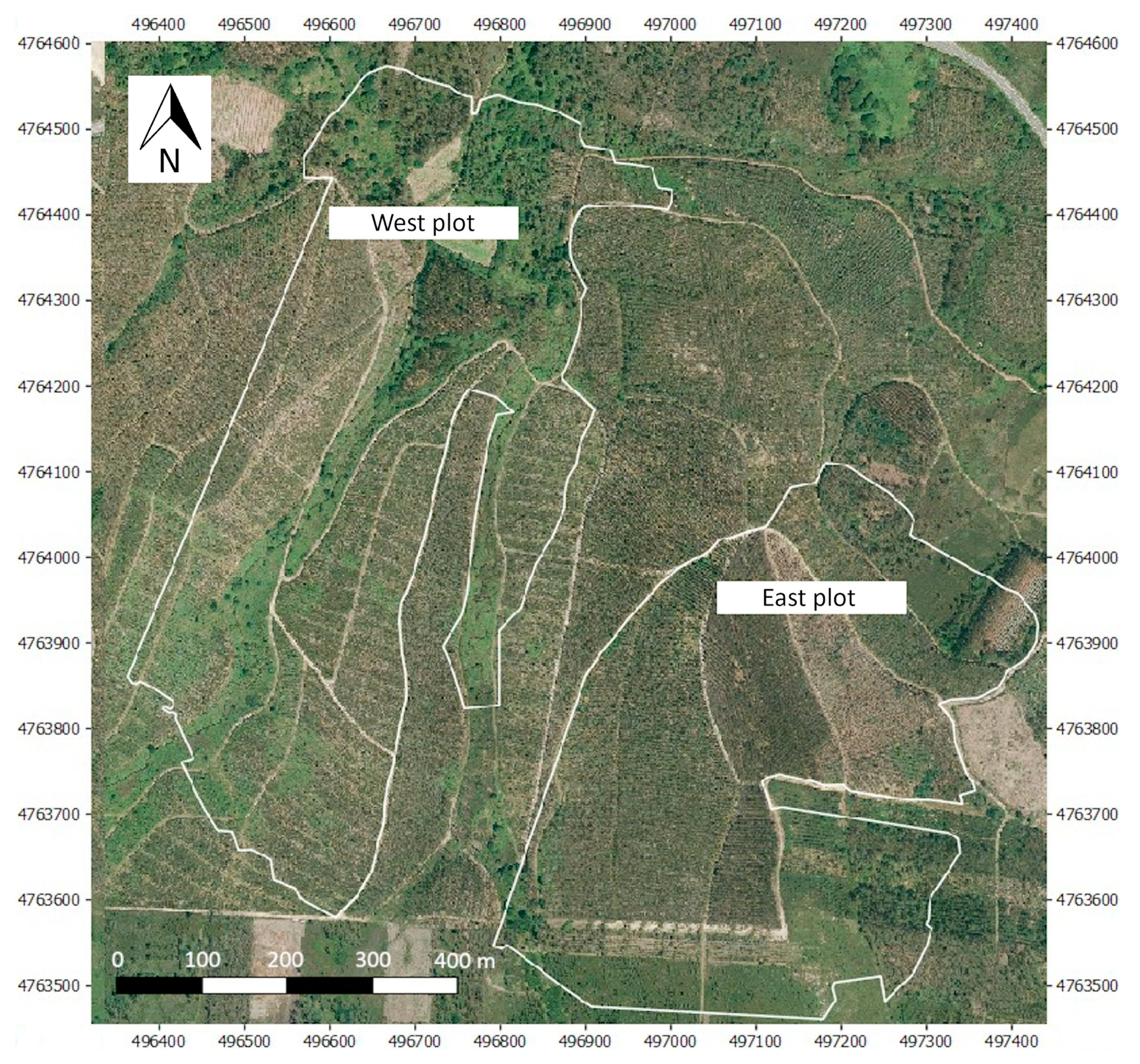
The study area is located in Galicia, Spain. Galicia is one of the European regions with higher forest productivity, ranging from 6 to 12 m3/ha/year, depending on the particular species [55], and supplies 4.5% of Europe’s timber [56]. With only 5.9% of the Spanish area, Galicia provides 54.3% of the national timber cutting [57]. In 2009, 21.9% of the Galician forestland consisted of Eucalyptus spp., primarily globulus and nitens spp. [58,59]. This accounts for circa 60%–70% of Spanish Eucalyptus cuttings [60], and accounted for approximately 50% of the Spanish production of chemical pulp over the period from 2008–2015 [61]. The study was performed in two Eucalyptus plots, the west plot and east plot of 34 ha and 25 ha, respectively (Figure 1). The elevation ranges from 324 m to 440 m and the slope from 0° to 69°. The tree spacing across the whole plantation was 2.0 × 4.0 m. Defoliation by the snout beetle affected both plots. Despite the uniform tree spacing in both plots, a number of paths and forest gaps were present across the scanned area, especially in the west one.
2.2. Data Acquisition and Pre-Processing
The aerial survey was conducted in 2017 above both studied plots. The LiDAR data were collected using the Matrice600-PRO multicopter, which was equipped with a VelodynePuck LITETM laser scanner. The LiDAR sensor had a measurement range of 100 m, an accuracy range up to 3 cm, and generated up to ~600,000 points/second at dual return mode across a 360° horizontal field of view and with a 30° vertical field of view. Rotation rate was 5 Hz–20 Hz and laser wavelength was 903 nm. The data were acquired by flying at 60 m above ground level with a programmed speed of 7 m/s. Direct georeferencing was applied using a STONEX S10 GNSS receiver. The final position accuracy was 1.5 cm in x–y and 2 cm in z.
The raw LiDAR data were filtered in order to delete the obtained noise. The point cloud resulted in a density of 55.2 points/m2 in the west plot and 67.0 points/m2 in the east plot. The next processing steps were performed using the available tools of LASTools software [62]. First, the ground points were identified using lasground, while the height of each point above the ground was computed using lasheight. Therefore, each point of the point cloud contains its X, Y, and normalized Z coordinates. After that process, it was possible to obtain a CHM of the study area. Two CHMs with different resolutions (0.5 m and 2.0 m) were directly created from the normalized point cloud. They were created using lasgrid tool with the option “-highest”, which assigns to each pixel the highest Z coordinate among all LiDAR points contained into the corresponding 0.5 m by 0.5 m (or 2.0 m by 2.0 m) cell.
2.3. Tree Detection and Tree Height Determination
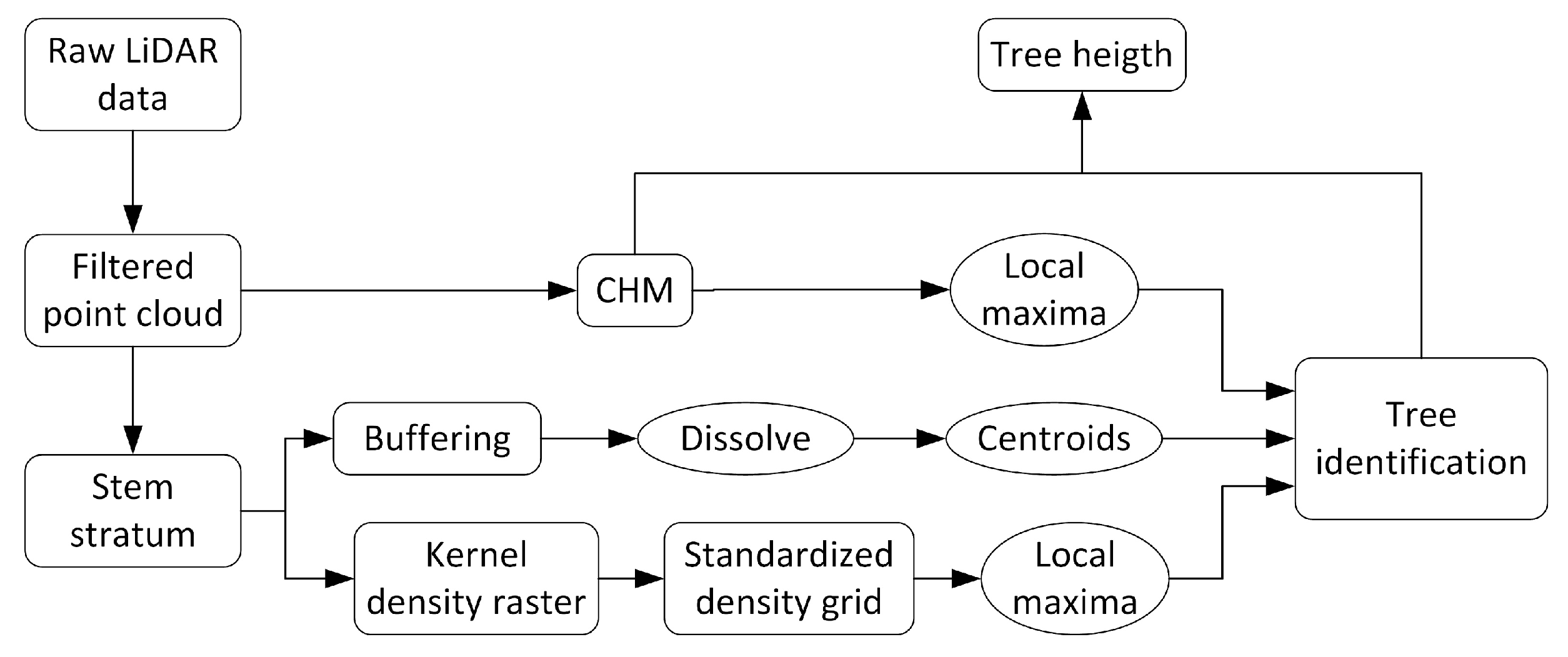
This work evaluates two procedures to calculate the number of Eucalyptus trees: Method 1 and Method 2. The results were compared to those obtained through the application of local maxima algorithms. Figure 2 presents the workflow followed.
Local maxima algorithms were applied using two softwares: Fusion [63] and Quantum Geographic Information System (QGIS) [64]. Fusion tool CanopyMaxima identifies local maxima on a CHM using a variable size evaluation window. Equations used to calculate the window size were specified in the Fusion User’s manual [65]. Default parameters were used to apply the algorithm to the study case. QGIS uses the local maxima and minimum algorithm [62]. Both algorithms were applied on CHM with different resolutions of 0.5 m and 2.0 m.
Instead of delineation of individual tree crowns, as in the CHM–LM methods, the proposed methods will attempt to delineate individual tree locations by classifying returns from the tree stems. The first step for these approaches is to extract the layer of points that correspond to the stems. To that end, threshold height values were used to classify the point cloud into vertical strata: ground, shrubs, stems, and canopy. Classification was performed on the normalized LiDAR point cloud using the lasheight tool from LASTools software [66]. Height thresholds are determined through point cloud visual inspection of the shrub stratum height and the crown base height for both analyzed plots. The adopted threshold values are shown in Table 2. They differ between plots as the west plot had taller shrubs and trees than the east plot.
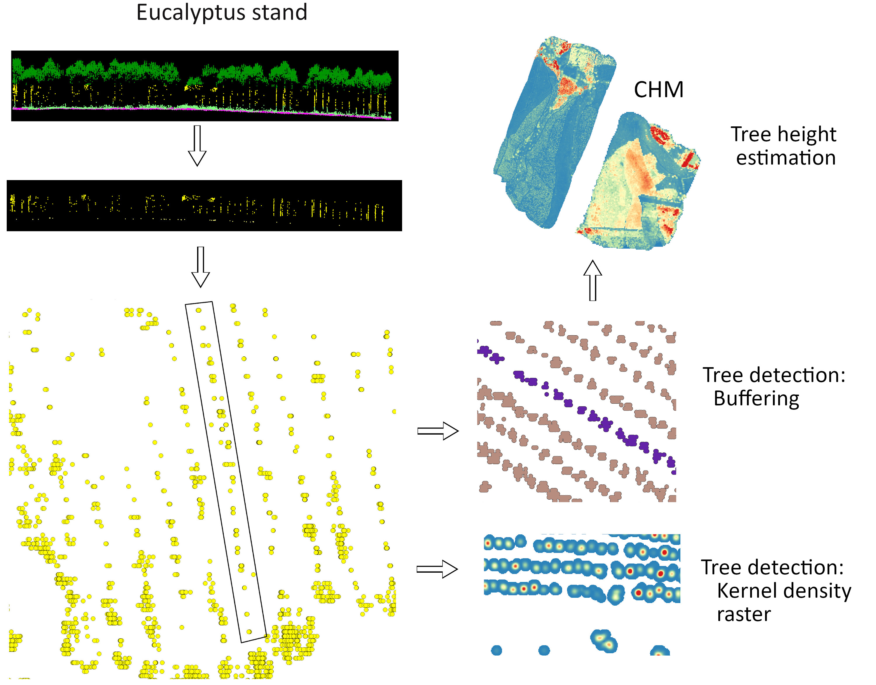
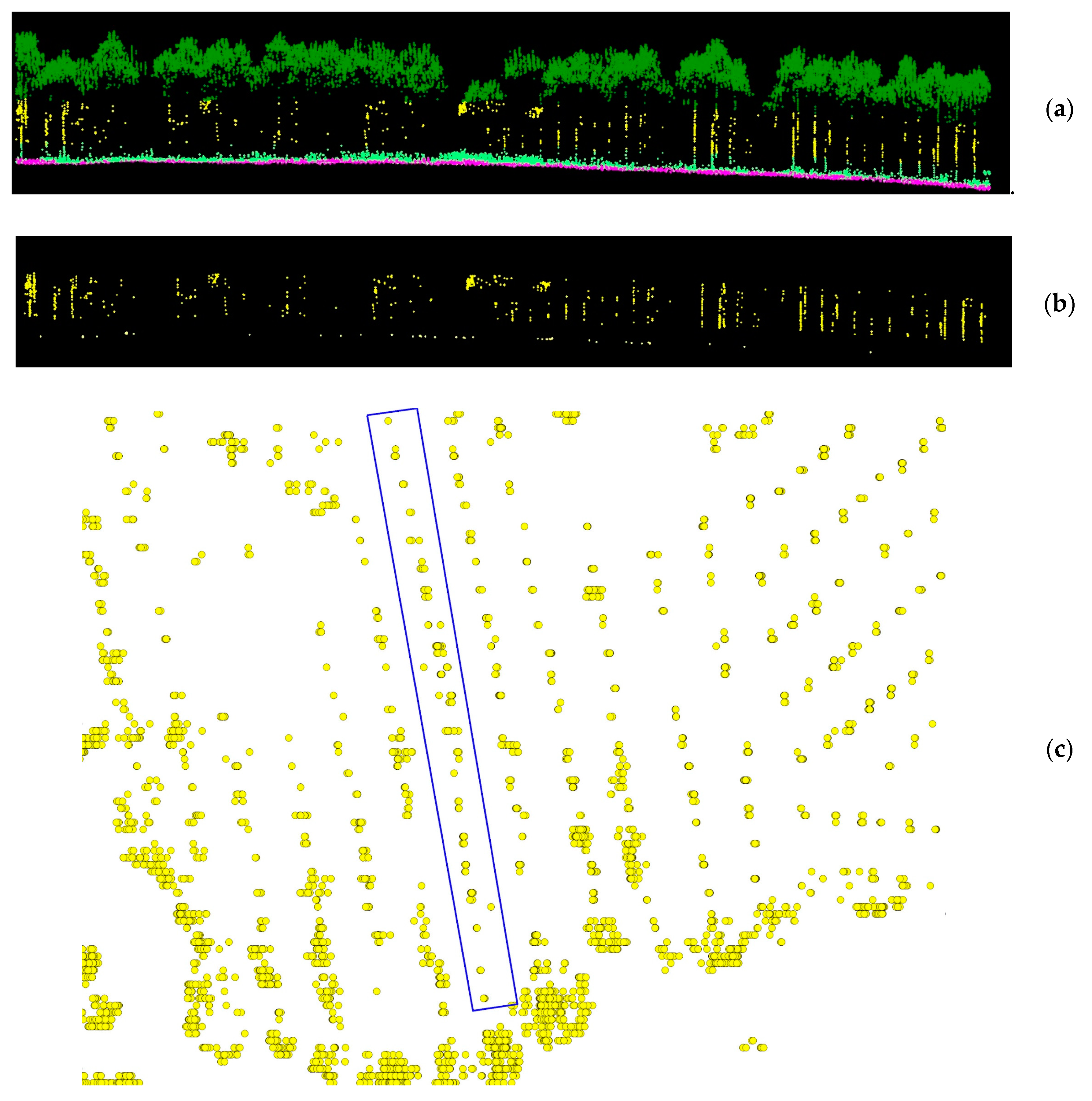
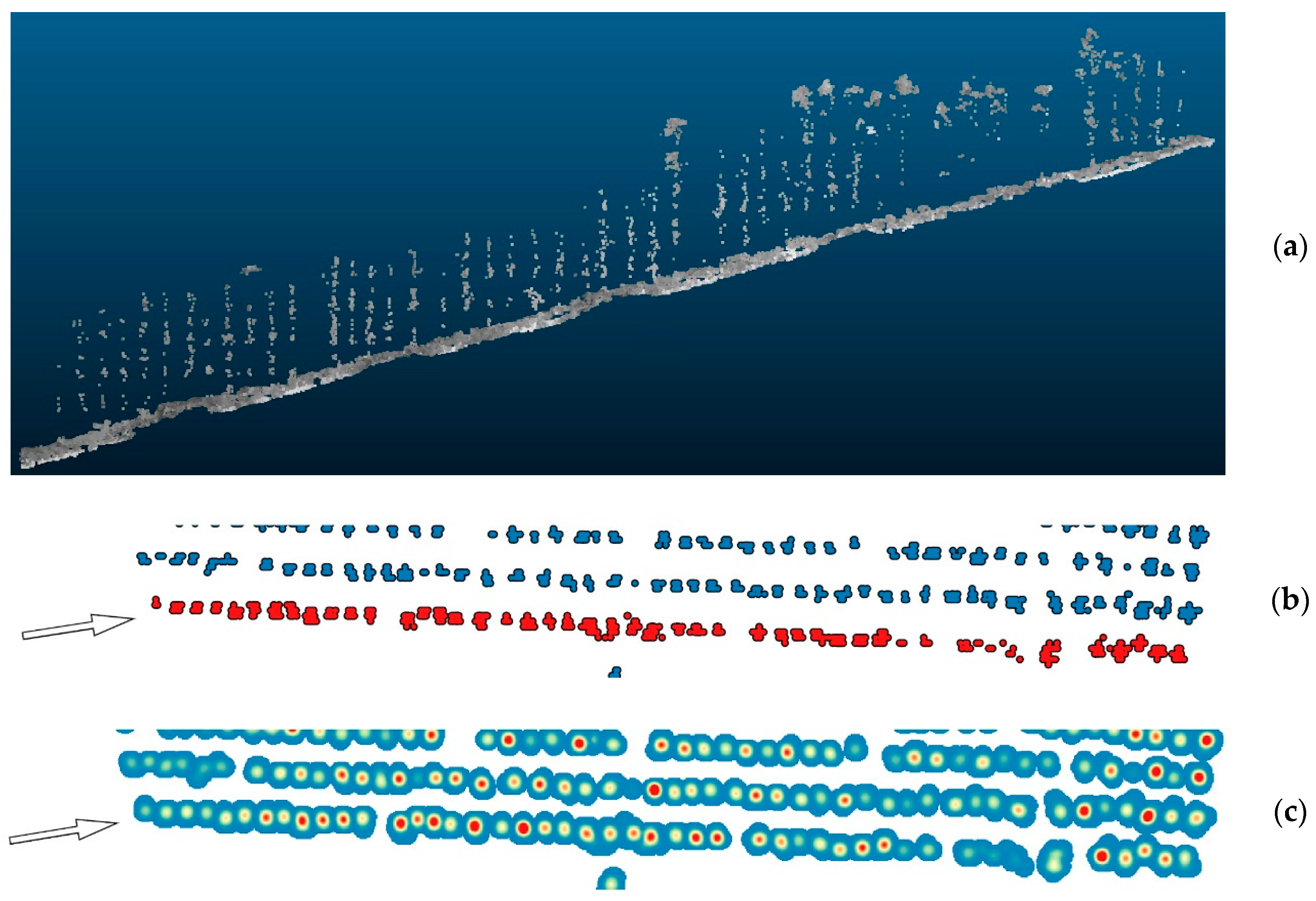
Afterward, the stem stratum is subset from the point cloud. Finally, the stem strata point cloud is projected in the horizontal plane. Figure 3 illustrates the described process. Figure 3a is an example of the point cloud classification step through a classified vertical profile of a single tree row. Figure 3b contains a front view of the segmented stem stratum. Finally, Figure 3c contains the horizontal projection of the stem stratum points.
Method 1 starts by creating a 2D buffer around each point of the projected stem point cloud. The buffer width must be above the X–Y point spacing and below the tree spacing. Several values were tested (0.30 m, 0.50 m, 1.00 m, 1.25 m). As a result, the point cloud was transformed into a cloud of polygons. Then, the buffers that intersected were combined into a single polygon. Figure 4b shows an example of the resulting polygons. Then, the cartographic coordinates X, Y of the centroid of the single polygons were obtained. These centroids approximate the geospatial position of every individual tree.
Method 2 is based on considering that a high point density in the horizontally projected point cloud of stems corresponds to an individual tree. The first step is the creation of a two-dimensional raster of the projected stem point cloud calculated from a kernel density estimation with an axis-aligned bivariate quartic kernel. The spatial resolution selected to create the raster was 0.1 m and the kernel radius was 1 m. In order to optimize high density areas, a standardization of the density grid was performed. Figure 4c provides an example of the standardized grid. Finally, a local maxima algorithm was applied to the resulting standardized grid. The result was a point set that corresponded to individual tree geolocation.
Once the tree detection methods were accomplished, the height analysis was performed. The height of each individual was estimated through the CHM. Thus, the center coordinates of each detected tree was intersected with the CHM to obtain the height value of each tree. Finally, all points under 5 m height were deleted, as they might correspond to shrubs. As a result of the detection methods, the position of the detected trees was obtained in the form of a set of points with cartographic coordinates. Thus, the CHM height value for those coordinates was extracted. This procedure was carried out using the CHM with a 0.5 m resolution and the CHM with a 2.0 m resolution.
2.4. Assessment of Methods
The evaluation of the accuracy in the tree detection of the analyzed methods was accomplished through visual inspection of the acquired point cloud before processing. Field work was not performed given the reduced accessibility through the analyzed stands due to the height of thorny shrubs (Ulex sp.). Seven tree rows were randomly selected in the study area, and the point cloud was segmented to isolate every row. The number of trees were manually counted in the front view of the point cloud corresponding to every sampled row plantation. This way, 242 trees were identified. Afterward, the DR of each method was calculated as the number of trees detected by the algorithm in the sample rows were divided by the total number of trees that were manually counted in the point cloud (242).
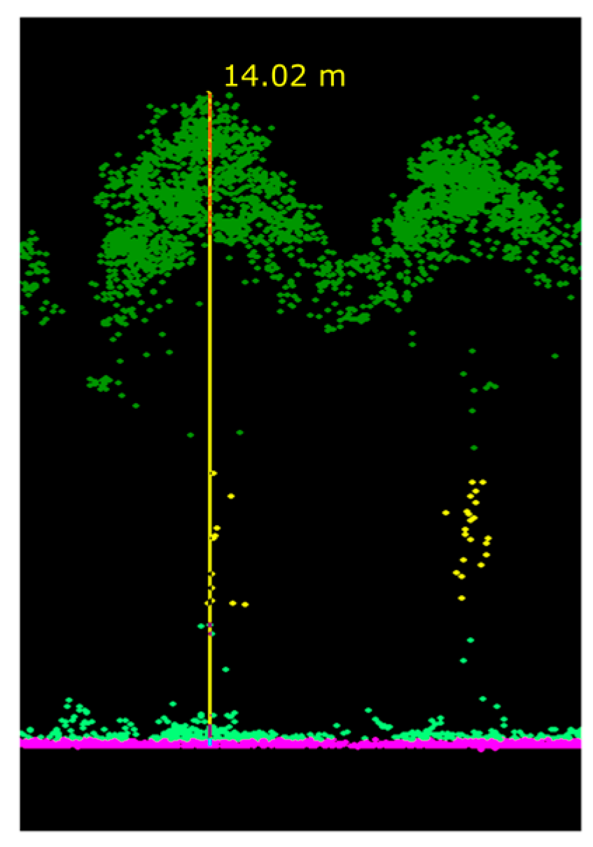
Finally, the verification of the height attribute was performed by measuring the point-to-point distance in the front view of the point cloud of a sample of randomly selected trees. Specifically, the considered sample consisted of 30 trees randomly distributed all over the study area. The measurement was done manually by selecting the apical point and a ground point placed just by the stem. An example of the measuring method is shown in Figure 5. The resulting values were compared to those obtained from the CHM.
3. Results
3.1. Tree detection
The numerical results of the tree detection and counting and associated predicted density are collected in Table 3. It should be remarked that, with regard to the final buffer value used in Method 1, the best performance was achieved with 0.30 m. With the other tested values, neighboring trees resulted in overlapped polygons. The higher the applied buffer value, the more this overlapping resulted.
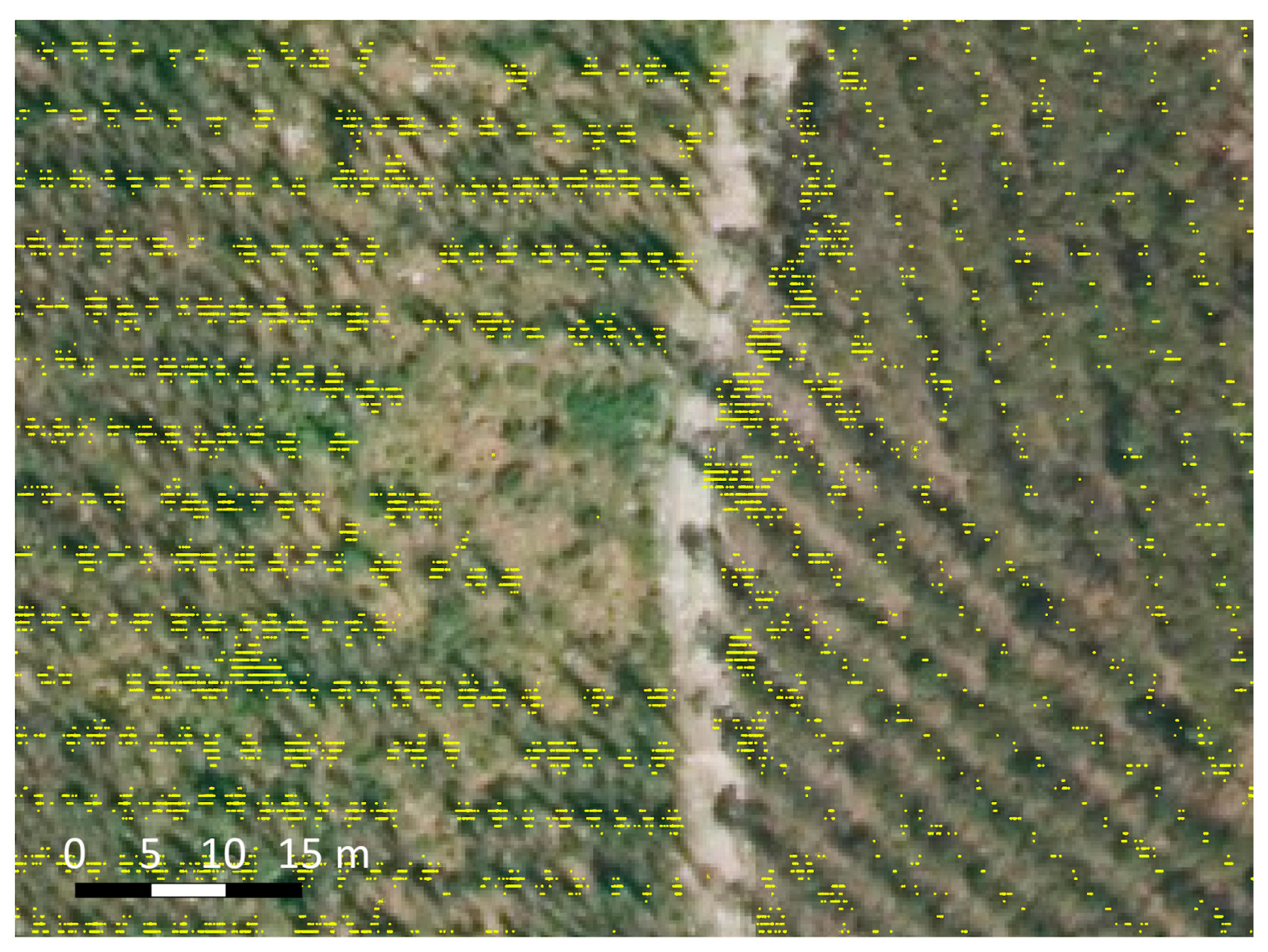
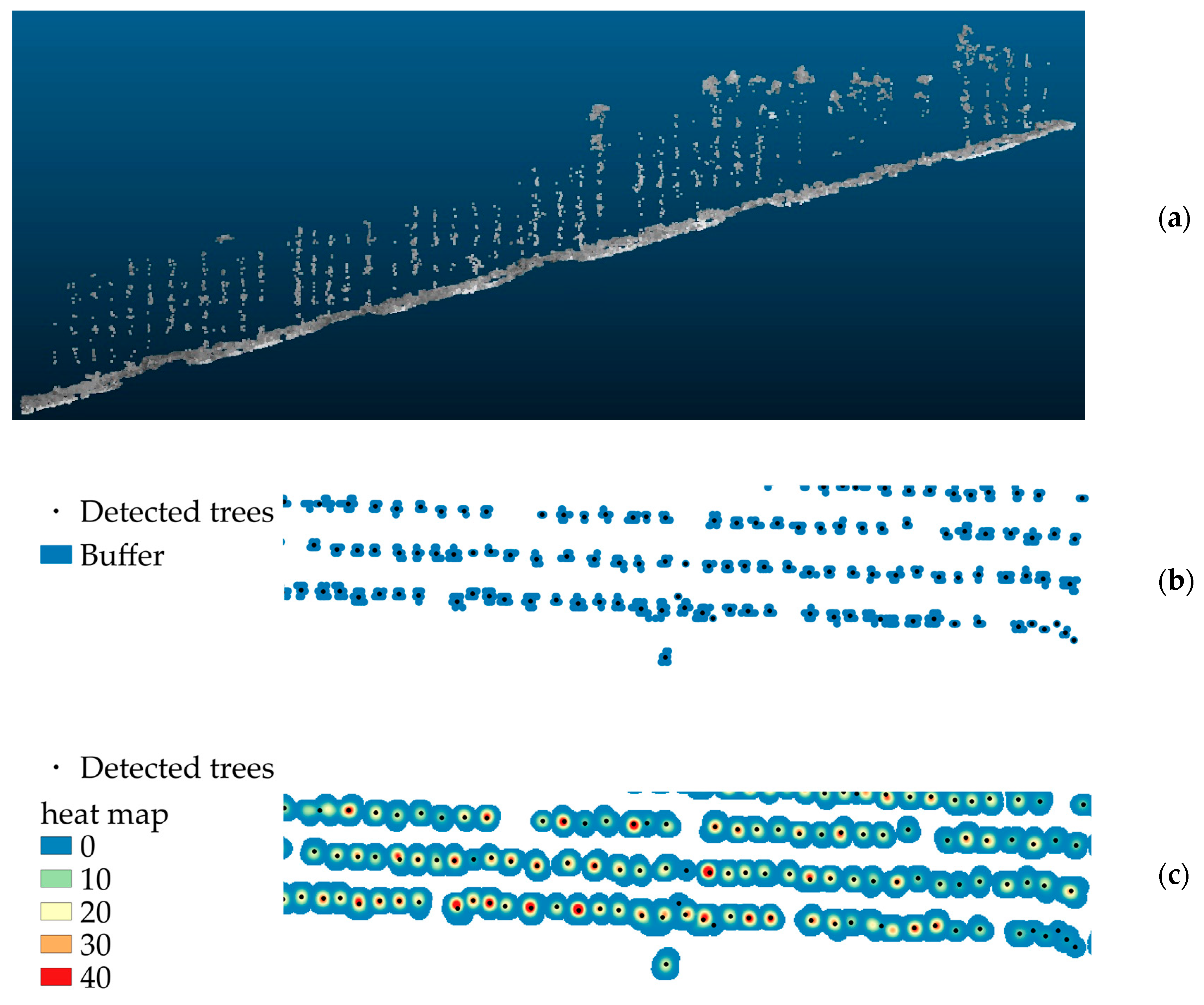
According to the average distance between the trees (2 m) and rows (4 m), the expected density should be 1250 trees/ha. The density provided by the ITD methods is below this value due to the presence of forest gaps (see Figure 6). CHM–LM with a 2.0 m pixel size provided the lowest number of trees, regardless of the algorithm used. An overview of the ITD results obtained by Method 1 and Method 2 is presented in Figure 7.
Although the number of detected trees gives an idea of the achieved results, a verification through visual interpretation on the point cloud was performed to gather accuracy metrics. The DR on the sampled rows is presented in Table 4. The DR for the CHM–LM with a 0.5 m pixel size using QGIS was 106.2%. However, Fusion CHM–LM at the same pixel size provided a DR of 21.5%. Both Method 1 and Method 2 overestimated the number of trees and provided a DR of 103.7% and 113.6%, respectively. Thus, false positives surpass false negatives.
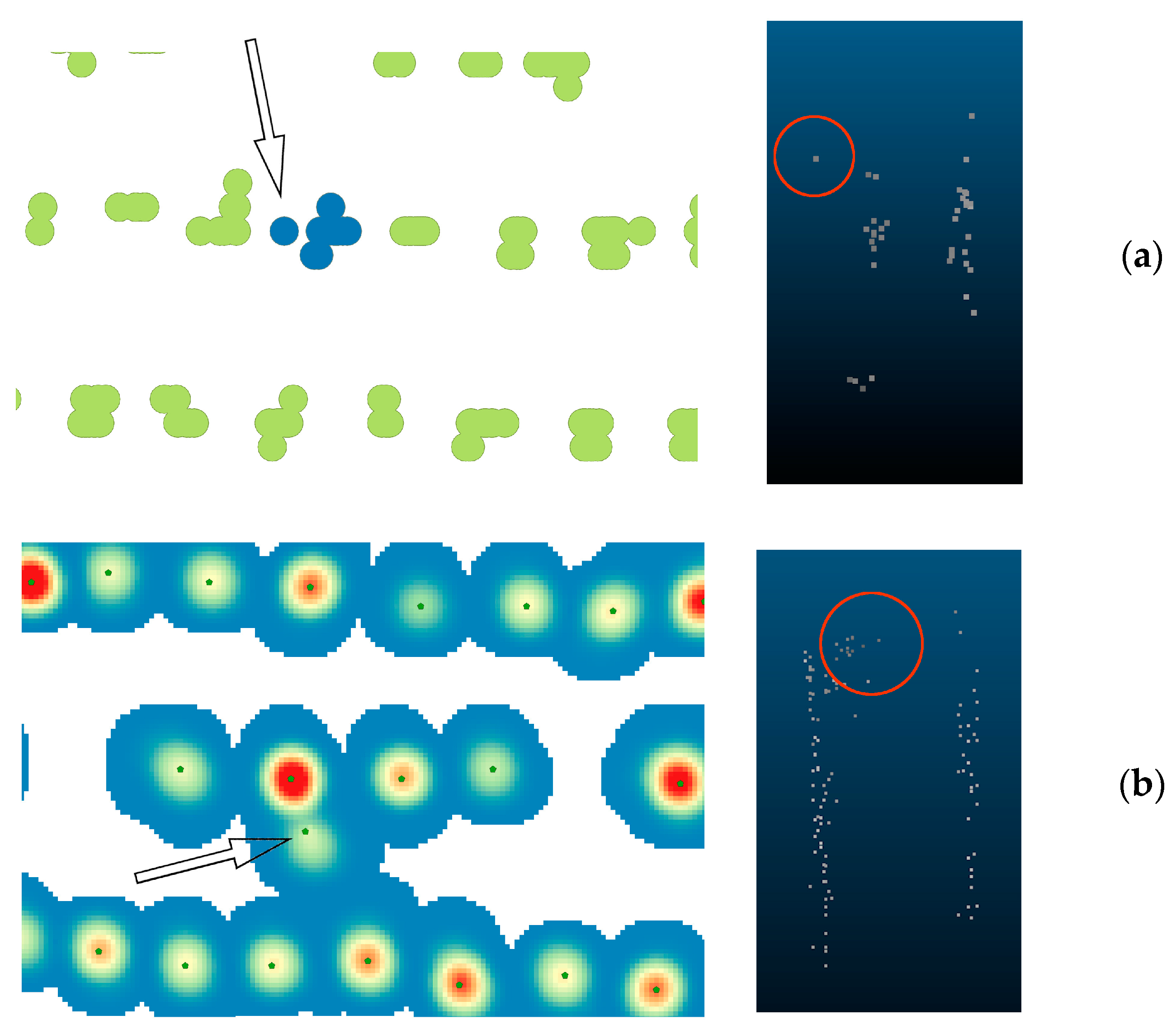
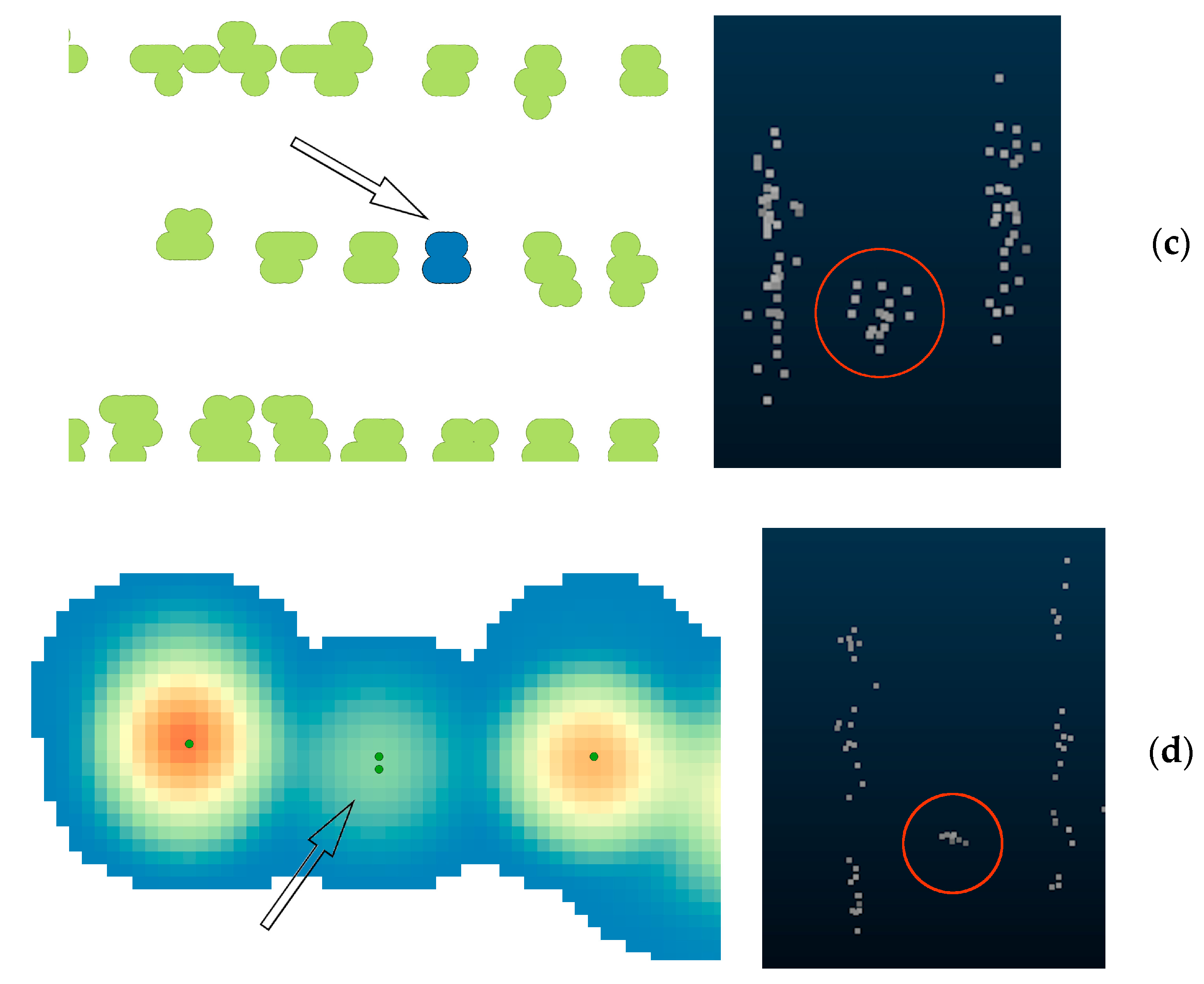
The visual analysis of the results allowed us to interpret error sources for Method 1 and Method 2. Some examples of commission errors are shown in Figure 8. In the case of Figure 8a, a single canopy return was identified as individual trees because the buffer distance was not large enough to reach the overlap with the corresponding tree. In Figure 8b, a group of points caused an extra local maximum in the density grid. These errors may be induced either by the multi-branch structure of Eucalyptus, or by the penetration of canopy in the stem layer. Similarly, Figure 8c,d correspond to false positives due to the incorporation of shrub returns to the stem layer or the presence of fallen snag trees. Again, Method 2 seems to be more prone to these types of errors.
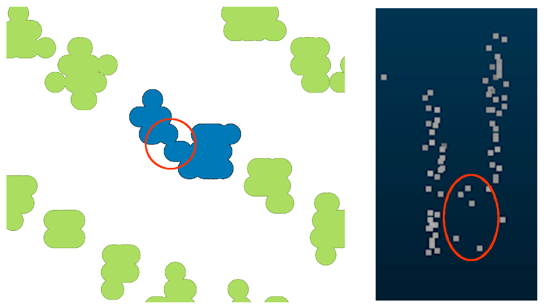
Omission errors were also checked through visual inspection. As an example, Figure 9 represents two stems that were detected as a single polygon in Method 1. In this particular case, the threshold values considered for the classification of the vegetation stratum did not allow for the complete separation of shrub and stems. Some points corresponding to shrub vegetation remained in the stem layer. As a result, the buffer distance dissolved two trees into a single polygon. This mechanism makes Method 1 more prone to false negatives.
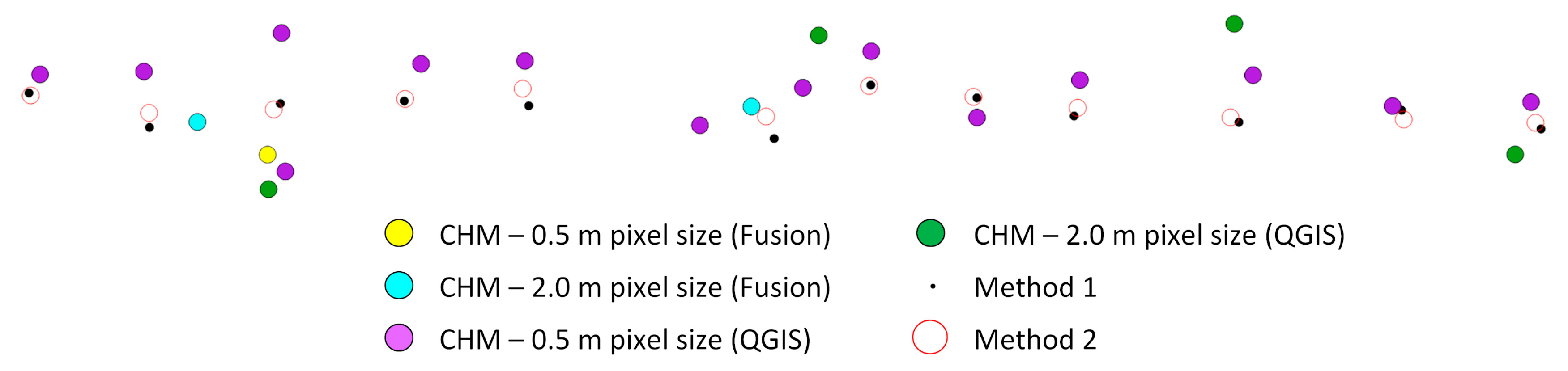
Once the stems were identified, their location coordinates could be obtained. Method 1 and Method 2 generated close coordinates, as can be appreciated in Figure 10. Conversely, the positions provided by the CHM–LM detection differ from them.
3.2. Tree Height Determination
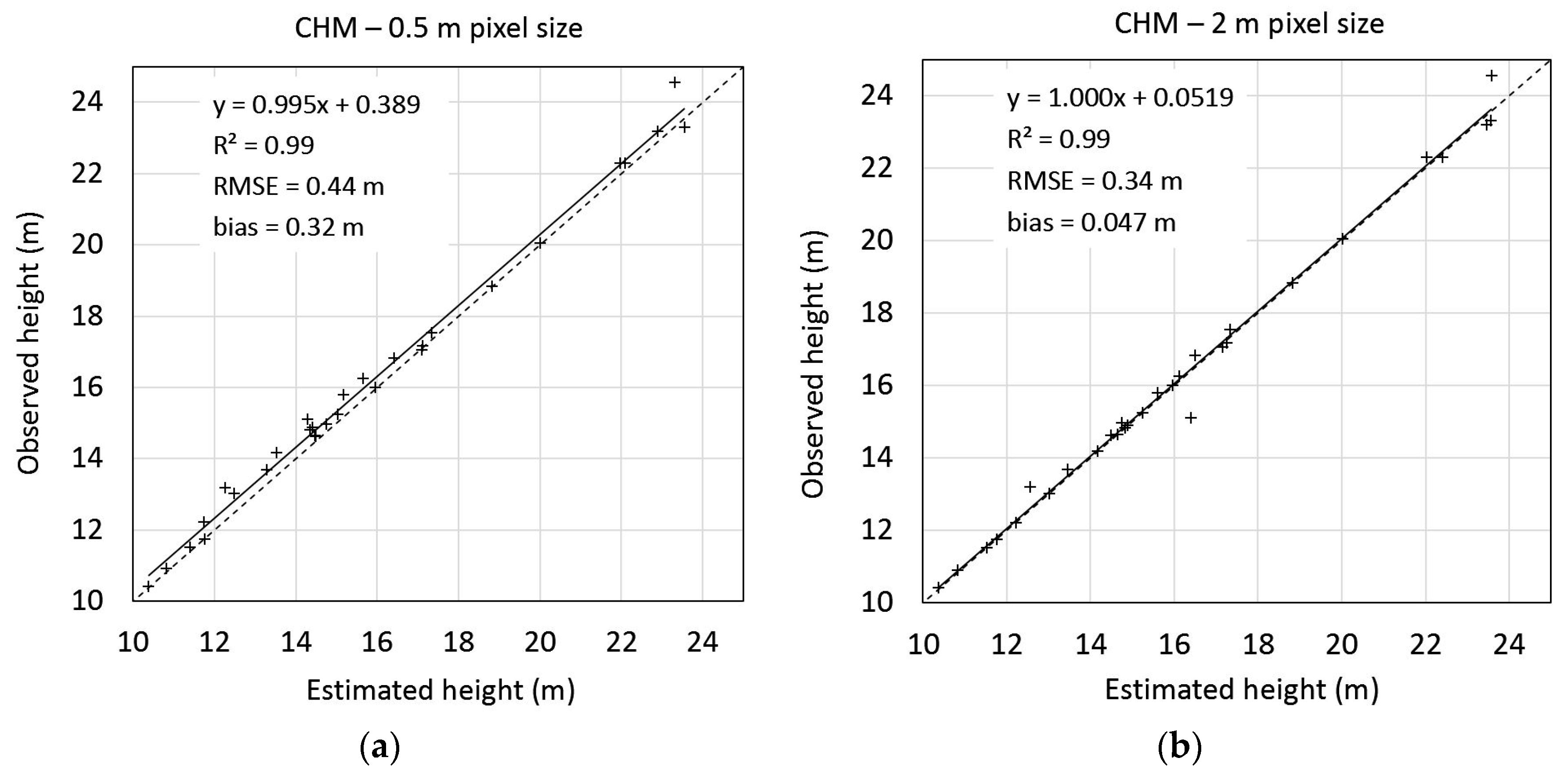
Finally, for each tree, its location coordinates were used to extract the corresponding height on the CHM. The CHM resolutions of 0.5 m and 2.0 m were also considered at the calculation of tree height. The height estimation was evaluated on a sample of three plantation rows. The ground truth values of the height were estimated directly in the original point cloud. The correlating parameters are collected in Figure 11.
The estimation of tree height values considering the 0.5 m CHM and 2.0 m CHM provide similar results in view of the RMSE and the R2 values.
4. Discussion
Method 1 and Method 2 provide accurate estimations of individual tree detection on Eucalyptus stands, independently of defoliation-related problems. The resulting DR with these methods is similar to the DR obtained in other studies that are focused on tree detection in Eucalyptus healthy stands: 92% [13], 97% [42], and 99% [43]. In the case of Wallace et al. [45], the DR resulted in an overestimation of 100.6% using a LM-based on a seeded k-means clustering approach. Method 1 and Method 2 also produced overestimated results (103.7% and 113.6%, respectively). The overview of the misinterpreted returns illustrates that the obtained errors were mostly linked to tall shrubs and snag trees. In addition, the crown base height of small trees was lower than the taller ones. This fact implies that tree branches of small trees may have penetrated into the generated stem layer, resulting in the misidentification of tree branches as single trees. In summary, most of the analyzed errors were related to the threshold values of height that were used to define the stem layer. These might be adapted to the vegetation of every analyzed plot in order to minimize commission errors and omission errors.
Finally, the accuracy of both methods depends on additional key inputs: the buffer distance and the search kernel radius used in generating the raster. Adequate values depend, above all, on two variables: tree spacing and point density. The presented results suggest that a higher point cloud density will allow a lower buffer distance and a lower search radius; consequently, the commission error will be minimized. Furthermore, the more spaced the trees are, the easier the tree isolation will be. Consequently, Method 1 is not expected to be valid in stands with no uniform spacing or low density stands.
Obtained results on tree height estimation show that the extraction of this attribute from both the CHM with a 0.5 × 0.5 m pixel size and CHM with a 2.0 × 2.0 m pixel size provided accurate estimations (R2 0.99 for both of them, and RMSE of 0.44 and 0.34, respectively). This might indicate that the stem is vertically aligned with the apical point of trees, which is reasonable for a high density plantation like the analyzed one. The obtained RMSE values were similar to those obtained in other studies. For example, Gonçalves-Seco et al. [41] obtained a RMSE of 1.91 m by applying the local maxima algorithm on a 0.5 m CHM obtained from a LiDAR point cloud of 4 points/m2. Sothe et al. [34] obtained a RMSE of 2.80 m estimating heights from a 0.2 m CHM using the CanopyMaxima tool from Fusion on a point cloud with 43.33 points/m2.
5. Conclusions
This work presents two methods to individually detect the stems of a Eucalyptus plantation by using UAV-LiDAR data. Both methods were based on the segmentation and processing of stem layer returns. The first (Method 1) is based on creating a buffer around stem returns. The second (Method 2) is based on also creating a kernel density raster on stem returns. Both methods allowed us to address an important barrier reported by other works: tree counting on broadleaves [67] stands and defoliated trees [41].
The results indicate that the proposed methods allow a high-accurate estimation of the number of trees to be obtained: there was a detection rate of 103.7% using Method 1 and 113.6% using Method 2. The accuracy of the proposed methods relies on the morphological uniformity of the analyzed stand: straight and unbranched stems, together with uniform age, height, and crown base height of individuals will provide better results. Vertical structure of the stand might also compromise the results. Shrub heights might be under crown base heights in absolute terms all over the stand. Further research could be oriented to assess the transferability of these methods on Eucalyptus stands with different structures and on different tree species. The presented methods may be automated to perform an individualized characterization in terms of height for every tree in the stand.
The presented study addressed stem counting and tree georeferencing in one of the most widely planted hardwoods in the world. The automated extraction of forest structural parameters is required to move toward precision forestry. Additionally, it could help to cover the lack of management tools for Eucalyptus stands reported by Crecente-Campo et al. [40]. In short, the proposed methodology provides the required accuracy to switch from area-based work to individual tree-based management.
Author Contributions
Conceptualization, J.P. and J.A.; Methodology, J.P. and J.A.; Software, D.M. and L.A.; Validation, L.A., D.M.; Formal analysis, J.P., J.A., G.B., and L.A.; Data curation, D.M. and L.A.; Writing—original draft preparation, G.B., J.A., and L.A.; Writing—review and editing, G.B., J.A., and L.A.; Supervision, J.A. and J.P. All authors have read and agreed to the published version of the manuscript.
Funding
This research received no external funding.
Conflicts of Interest
The authors declare no conflicts of interest.
References
- Li, J.; Hu, B.; Noland, T.L. Classification of tree species based on structural features derived from high density LiDAR data. Agric. For. Meteorol. 2013, 171, 104–114. [Google Scholar] [CrossRef]
- Edson, C.; Wing, M.G. Airborne Light Detection and Ranging (LiDAR) for individual tree stem location, height, and biomass measurements. Remote Sens. 2011, 3, 2494–2528. [Google Scholar] [CrossRef] [Green Version]
- Bouvier, M.; Durrieu, S.; Fournier, R.A.; Renaud, J.-P. Generalizing predictive models of forest inventory attributes using an area-based approach with airborne LiDAR data. Remote Sens. Environ. 2015, 156, 322–334. [Google Scholar] [CrossRef]
- Wulder, M.A.; White, J.C.; Nelson, R.F.; Næsset, E.; Ørka, H.O.; Coops, N.C.; Hilker, T.; Bater, C.W.; Gobakken, T. Lidar sampling for large-area forest characterization: A review. Remote Sens. Environ. 2012, 121, 196–209. [Google Scholar] [CrossRef] [Green Version]
- Maltamo, M.; Næsset, E.; Vauhkonen, J. Forestry Applications of Airborne Laser Scanning: Concepts and Case Studies; Springer: Dordrecht, The Netherlands, 2014. [Google Scholar] [CrossRef]
- Hyyppä, J.; Hyyppä, H.; Leckie, D.; Gougeon, F.; Yu, X.; Maltamo, M. Review of methods of small-footprint airborne laser scanning for extracting forest inventory data in boreal forests. Int. J. Remote Sens. 2008, 29, 1339–1366. [Google Scholar] [CrossRef]
- Budei, B.C.; St-Onge, B.; Hopkinson, C.; Audet, F.-A. Identifying the genus or species of individual trees using a three-wavelength airborne lidar system. Remote Sens. Environ. 2018, 204, 632–647. [Google Scholar] [CrossRef]
- Stone, C.; Webster, M.; Osborn, J.; Iqbal, I. Alternatives to LiDAR-derived canopy height models for softwood plantations: A review and example using photogrammetry. Aust. For. 2016, 79, 271–282. [Google Scholar] [CrossRef]
- Shinzato, E.T.; Shimabukuro, Y.E.; Coops, N.C.; Tompalski, P.; Gasparoto, E.A. Integrating area-based and individual tree detection approaches for estimating tree volume in plantation inventory using aerial image and airborne laser scanning data. iFor. Biogeosci. For. 2017, 10, 296–302. [Google Scholar] [CrossRef] [Green Version]
- Jeronimo, S.M.A.; Kane, V.R.; Churchill, D.J.; McGaughey, R.J.; Franklin, J.F. Applying LiDAR individual tree detection to management of structurally diverse forest landscapes. J. For. 2018, 116, 336–346. [Google Scholar] [CrossRef] [Green Version]
- Næsset, E. Estimating timber volume of forest stands using airborne laser scanner data. Remote Sens. Environ. 1997, 61, 246–253. [Google Scholar] [CrossRef]
- Næsset, E. Predicting forest stand characteristics with airborne scanning laser using a practical two-stage procedure and field data. Remote Sens. Environ. 2002, 80, 88–99. [Google Scholar] [CrossRef]
- Cosenza, D.N.; Soares, V.P.; Leite, H.G.; Gleriani, J.M.; Amaral, C.H.d.; GrippJúnior, J.; Silva, A.A.L.d.; Soares, P.; Tomé, M. Airborne laser scanning applied to eucalyptus stand inventory at individual tree level. Pesqui. Agropecu. Bras. 2018, 53, 1373–1382. [Google Scholar] [CrossRef]
- Chen, Q.; Baldocchi, D.; Gong, P.; Kelly, M. Isolating individual trees in a savanna woodland using small footprint lidar data. Photogramm. Eng. RemoteSens. 2006, 72, 923–932. [Google Scholar] [CrossRef] [Green Version]
- Wulder, M.A.; Bater, C.W.; Coops, N.C.; Hilker, T.; White, J.C. The role of LiDAR in sustainable forest management. For. Chron. 2008, 84, 807–826. [Google Scholar] [CrossRef] [Green Version]
- Liu, Q.; Li, Z.; Chen, E.; Pang, Y.; Tian, X.; Cao, C. Estimating biomass of individual trees using point cloud data of airborne LIDAR. Chin. High. Technol. Lett. 2010, 20, 765–770. [Google Scholar]
- Morsdorf, F.; Meier, E.; Kötz, B.; Itten, K.I.; Dobbertin, M.; Allgöwer, B. LIDAR-based geometric reconstruction of boreal type forest stands at singletree level for forest and wildland fire management. Remote Sens. Environ. 2004, 92, 353–362. [Google Scholar] [CrossRef]
- Khosravipour, A.; Skidmore, A.K.; Isenburg, M. Generating spike-free digital surface models using LiDAR raw point clouds: A new approach for forestry applications. Int. J. Appl. Earth Obs. Geoinf. 2016, 52, 104–114. [Google Scholar] [CrossRef]
- Iglhaut, J.; Cabo, C.; Puliti, S.; Piermattei, L.; O’Connor, J.; Rosette, J. Structure from Motion Photogrammetry in Forestry: A review. Curr. For. Reports. 2019, 5, 155–168. [Google Scholar] [CrossRef] [Green Version]
- Goodbody, T.R.H.; Coops, N.C.; White, J.C. Digital Aerial Photogrammetry for Updating Area-Based Forest Inventories: A Review of Opportunities, Challenges, and Future Directions. Curr. For. Reports. 2019, 5, 55–75. [Google Scholar] [CrossRef] [Green Version]
- Wallace, L.; Lucieer, A.; Malenovský, Z.; Turner, D.; Vopěnka, P. Assessment of Forest Structure Using Two UAV Techniques: A Comparison of Airborne Laser Scanning and Structure from Motion (SfM) Point Clouds. Forests 2016, 7, 62. [Google Scholar] [CrossRef] [Green Version]
- Zhao, K.; Popescu, S. Hierarchical watershed segmentation of canopy height model for multi-scale forest inventory. In Proceedings of the ISPRS Workshop on Laser Scanning 2007 and SilviLaser 2007, Espoo, Finland, 12–14 September 2007; Volume XXXVI. Part3/W52. [Google Scholar]
- Bortolot, Z.J.; Wynne, R.H. Estimating forest biomass using small footprint LiDAR data: An individual tree-based approach that incorporates training data. ISPRS J. Photogramm. Remote Sens. 2005, 59, 342–360. [Google Scholar] [CrossRef]
- Mohan, M.; Silva, A.C.; Klauberg, C.; Jat, P.; Catts, G.; Cardil, A.; Hudak, T.A.; Dia, M. Individual tree detection from Unmanned Aerial Vehicle (UAV) derived Canopy Height Model in an open canopy mixed conifer forest. Forests 2017, 8, 340. [Google Scholar] [CrossRef] [Green Version]
- Harikumar, A.; Bovolo, F.; Bruzzone, L. A local projection-based approach to individual tree detection and 3-D crown delineation in multistoried coniferous forests using high-density airborne LiDAR data. IEEE Trans. Geosci. Remote Sens. 2019, 57, 1168–1182. [Google Scholar] [CrossRef]
- Li, W.; Guo, Q.; Jakubowski, M.K.; Kelly, M. A new method for segmenting individual trees from the Lidar point cloud. Photogramm. Eng. Remote Sens. 2012, 78, 75–84. [Google Scholar] [CrossRef] [Green Version]
- Chen, Q.; Gong, P.; Baldocchi, D.; Tian, Y.Q. Estimating basal area and stem volume for individual trees from Lidar data. Photogramm. Eng. Remote Sens. 2007, 73, 1355–1365. [Google Scholar] [CrossRef] [Green Version]
- Korpela, I.; Dahlin, B.; Schäfer, H.; Bruun, E.; Haapaniemi, F.; Honkasalo, J.; Ilvesniemi, S.; Kuutti, V.; Linkosalmi, M.; Mustonen, J.; et al. Single-tree forest inventory using LIDAR and aerial images for 3D treetop positioning, species recognition, height and crown width estimation. Proc. IAPRS 2007, 36, 227–233. [Google Scholar]
- Yu, X.; Hyyppä, J.; Vastaranta, M.; Holopainen, M.; Viitala, R. Predicting individual tree attributes from airborne laser point clouds based on the random forests technique. ISPRS J. Photogramm. Remote Sens. 2011, 66, 28–37. [Google Scholar] [CrossRef]
- Gleason, C.J.; Im, J. A review of remote sensing of forest biomass and biofuel: Options for small-area applications. GISci. Remote Sens. 2011, 48, 141–170. [Google Scholar] [CrossRef]
- Falkowski, M.J.; Smith, A.M.S.; Hudak, A.T.; Gessler, P.E.; Vierling, L.A.; Crookston, N.L. Automated estimation of individual conifer tree height and crown diameter via two-dimensional spatial wavelet analysis of Lidar data. Can. J. Remote Sens. 2006, 32, 153–161. [Google Scholar] [CrossRef] [Green Version]
- Goerndt, M.E.; Monleon, V.J.; Temesgen, H. Relating forest attributes with area- and tree-based light detection and ranging metrics for Western Oregon. West. J. Appl. For. 2010, 25, 105–111. [Google Scholar] [CrossRef] [Green Version]
- Véga, C.; Durrieu, S. Multi-level filtering segmentation to measure individual tree parameters based on Lidar data: Application to a mountainous forest with heterogeneous stands. Int. J. Appl. Earth Obs. Geoinf. 2011, 13, 646–656. [Google Scholar] [CrossRef] [Green Version]
- Sothe, C.; Dalponte, M.; Almeida, M.C.; Schimalski, B.M.; Lima, L.C.; Liesenberg, V.; Miyoshi, T.G.; Tommaselli, M.A. Tree species classification in a highly diverse subtropical forest integrating UAV-based photogrammetric point cloud and hyperspectral data. Remote Sens. 2019, 11, 1338. [Google Scholar] [CrossRef] [Green Version]
- Zhen, Z.; Quackenbush, J.L.; Zhang, L. Trends in automatic individual tree crown detection and delineation—Evolution of LiDAR data. Remote Sens. 2016, 8, 333. [Google Scholar] [CrossRef] [Green Version]
- Donoghue, D.N.M.; Watt, P.J.; Cox, N.J.; Wilson, J. Remote sensing of species mixtures in conifer plantations using LiDAR height and intensity data. Remote Sens. Environ. 2007, 110, 509–522. [Google Scholar] [CrossRef]
- Rockwood, L.D.; Rudie, W.A.; Ralph, A.S.; Zhu, Y.J.; Winandy, E.J. Energy product options for Eucalyptus species grown as short rotation woody crops. Int. J. Mol. Sci. 2008, 9, 1361. [Google Scholar] [CrossRef] [PubMed]
- Food and Agriculture Organization (FAO) of the United Nations. Global Forest Resources Assessment 2005—Main Report; FAO Forestry Paper; FAO: Rome, Italy, 2005. [Google Scholar]
- McMahon, D.E.; Jackson, R.B. Management intensification maintains wood production over multiple harvests in tropical Eucalyptus plantations. Ecol. Appl. 2019, 29, e01879. [Google Scholar] [CrossRef]
- Crecente-Campo, F.; Tomé, M.; Soares, P.; Diéguez-Aranda, U. A generalized nonlinear mixed-effects height–diameter model for Eucalyptus globulus L. in northwestern Spain. For. Ecol. Manag. 2010, 259, 943–952. [Google Scholar] [CrossRef] [Green Version]
- Gonçalves-Seco, L.; González-Ferreiro, E.; Diéguez-Aranda, U.; Fraga-Bugallo, B.; Crecente, R.; Miranda, D. Assessing the attributes of high-density Eucalyptus globulus stands using airborne laser scanner data. Int. J. Remote Sens. 2011, 32, 9821–9841. [Google Scholar] [CrossRef]
- Guerra-Hernández, J.; Cosenza, D.N.; Rodriguez, L.C.E.; Silva, M.; Tomé, M.; Díaz-Varela, R.A.; González-Ferreiro, E. Comparison of ALS- and UAV (SfM)-derived high-density point clouds for individual tree detection in Eucalyptus plantations. Int. J. Remote Sens. 2018, 39, 5211–5235. [Google Scholar] [CrossRef]
- Oliveira, L.T.d.; Carvalho, L.M.T.d.; Ferreira, M.Z.; Oliveira, T.C.d.A.; Batista, V.T.F.P. Influência da idade na contagem de árvores de Eucalyptussp. com dados de Lidar (Portuguese). Cerne 2014, 20, 557–565. [Google Scholar] [CrossRef] [Green Version]
- Ferraz, A.; Bretar, F.; Jacquemoud, S.; Gonçalves, G.; Pereira, L.; Tomé, M.; Soares, P. 3-D mapping of a multi-layered Mediterranean forest using ALS data. Remote Sens. Environ. 2012, 121, 210–223. [Google Scholar] [CrossRef]
- Wallace, L.; Lucieer, A.; Watson, C.S. Evaluating tree detection and segmentation routines on very high resolution UAV LiDAR data. IEEE Trans. Geosci. Remote Sens. 2014, 52, 7619–7628. [Google Scholar] [CrossRef]
- Torresan, C.; Berton, A.; Carotenuto, F.; Chiavetta, U.; Miglietta, F.; Zaldei, A.; Gioli, B. Development and Performance Assessment of a Low-Cost UAV Laser Scanner System (LasUAV). Remote Sens. 2018, 10, 1094. [Google Scholar] [CrossRef] [Green Version]
- Zhou, J.; Proisy, C.; Descombes, X.; Le Maire, G.; Nouvellon, Y.; Stape, J.-L.; Viennois, G.; Zerubia, J.; Couteron, P. Mapping local density of young Eucalyptus plantations by individual tree detection in high spatial resolution satellite images. For. Ecol. Manag. 2013, 301, 129–141. [Google Scholar] [CrossRef] [Green Version]
- Amon, P.; Riegl, U.; Rieger, P.; Pfennigbauer, M. UAV-based laser scanning to meet special challenges in LiDAR surveying. In Proceedings of the Geomatics Indaba 2015—Stream 2, Ekurhuleni, South Africa, 11–13 August 2015; pp. 138–147. [Google Scholar]
- Liu, Q.; Li, S.; Li, Z.; Fu, L.; Hu, K. Review on the Applications of UAV-Based LiDAR and Photogrammetry in Forestry. Sci. Silvae Sin. 2017, 53, 134–148. [Google Scholar] [CrossRef]
- Petrie, G. Current developments in airborne laser scanners suitable for use on lightweight UAVs: Progress is being made! GeoInformatics 2013, 16, 16–22. [Google Scholar]
- Pilarska, M.; Ostrowski, W.; Bakuła, K.; Górski, K.; Kurczyński, Z. The potential of light laser scanners developed for unmanned aerial vehicles—The review and accuracy. Int. Arch. Photogramm. Remote Sens. Spat. Inf. Sci. 2016, 42, 87–95. [Google Scholar] [CrossRef] [Green Version]
- Salach, A.; Bakuła, K.; Pilarska, M.; Ostrowski, W.; Górski, K.; Kurczyński, Z. Accuracy assessment of point clouds from LiDAR and dense image matching acquired using the UAV platform for DTM creation. ISPRS Int. J. GeoInf. 2018, 7, 342. [Google Scholar] [CrossRef] [Green Version]
- Barnes, C.; Balzter, H.; Barrett, K.; Eddy, J.; Milner, S.; Suárez, C.J. Individual tree crown delineation from airborne laser scanning for diseased larch forest Ssands. Remote Sens. 2017, 9, 231. [Google Scholar] [CrossRef] [Green Version]
- Xunta de Galicia; Instituto Gallego de Promoción Económica (IGAPE). Oportunidades Industria 4.0 en Galicia—Diagnóstico Sectorial: Madera/Forestal (Spanish); 2017. Available online: http://www.igape.es/es/ser-mas-competitivo/galiciaindustria4-0/estudos-e-informes/item/download/58_60810179c81085089705d6dc680b42e7 (accessed on 15 October 2019).
- Chas Amil, M.L. Forest fires in Galicia (Spain): Threats and challenges for the future. J. For. Econ. 2007, 13, 1–5. [Google Scholar] [CrossRef]
- Jiménez, E.; Vega, J.A.; Fernández-Alonso, J.M.; Vega-Nieva, D.; Ortiz, L.; López-Serrano, P.M.; López-Sánchez, C.A. Estimation of aboveground forest biomass in Galicia (NW Spain) by the combined use of LiDAR, LANDSAT ETM+ and National Forest Inventory data. IFor. Biogeosci. For. 2017, 10, 590–596. [Google Scholar] [CrossRef]
- Gobierno de España; Ministerio de Agricultura Pesca y Alimentación. Avance de Estadística Forestal 2017 (Spanish); Centro de Publicaciones del Ministerio de Agricultura, Pesca y Alimentación: Madrid, Spain, 2017. [Google Scholar]
- Xunta de Galicia; Consellería do Medio Rural. 1a Revisión del Plan Forestal de Galicia. Documento de diagnóstico del monte y el sector forestal gallego (Spanish); 2018. Available online: https://mediorural.xunta.gal/sites/default/files/temas/forestal/plan-forestal/1_REVISION_PLAN_FORESTAL_CAST.pdf (accessed on 22 October 2019).
- Picos, J. Producción de eucalipto en Galicia. Guía de supervivencia. In Proceedings of the Jornadas CIDEU (Spanish), Huelva, Spain, 21–23 October 2009. [Google Scholar]
- Corbelle Rico, E.J.; Tubío Sánchez, J.M. Productivismo y abandono: Dos caras de la transición forestal en Galicia (España), 1966–2009 (Spanish). Bosque (Valdivia) 2018, 39, 457–467. [Google Scholar] [CrossRef] [Green Version]
- Álvarez-Díaz, M.; González-Gómez, M.; Otero-Giráldez, M.S. Main determinants of export-oriented bleached Eucalyptus kraft pulp (BEKP) demand from the north-western regions of Spain. For. Policy Econ. 2018, 96, 112–119. [Google Scholar] [CrossRef]
- Rapidlasso GmbH. LASTools. Available online: https://rapidlasso.com//lastools (accessed on 27 June 2019).
- Pacific Northwest Research Station—USDA Forest Service FUSION/LDV LIDAR Analysis and Visualization Software. Available online: http://forsys.sefs.uw.edu/FUSION/fusion_overview.html (accessed on 4 November 2019).
- QGIS—A Free and Open Source Geographic Information System. Available online: https://qgis.org (accessed on 18 February 2019).
- McGaughey, R.J. FUSION/LDV: Software for LIDAR Data Analysis and Visualization. 2018. Available online: http://forsys.sefs.uw.edu/Software/FUSION/FUSION_manual.pdf (accessed on 23 October 2019).
- Conrad, O.; Bechtel, B.; Bock, M.; Dietrich, H.; Fischer, E.; Gerlitz, L.; Wehberg, J.; Wichmann, V.; Böhner, J. System for Automated Geoscientific Analyses (SAGA) v. 2.1.4. Geosci. Model. Dev. 2015, 8, 1991–2007. [Google Scholar] [CrossRef] [Green Version]
- Huang, H.; Gong, P.; Cheng, X.; Clinton, N.; Li, Z. Improving measurement of forest structural parameters by co-registering of high resolution aerial imagery and low density LiDAR data. Sensors 2009, 9, 1541. [Google Scholar] [CrossRef]
Figure 1.
Location of the studied plots (aerial image from Plan Nacional de Ortofotografía Aérea (PNOA) 2016, https://pnoa.ign.es).
Figure 1.
Location of the studied plots (aerial image from Plan Nacional de Ortofotografía Aérea (PNOA) 2016, https://pnoa.ign.es).

Figure 2.
Flow chart for the three methods of individual tree detection.

Figure 3.
Extraction of the stem layer in a sample row of trees: (a) point cloud; (b) stem layer extraction from the point cloud; (c) horizontal projection of the extracted layer.
Figure 3.
Extraction of the stem layer in a sample row of trees: (a) point cloud; (b) stem layer extraction from the point cloud; (c) horizontal projection of the extracted layer.

Figure 4.
Overview of Method 1 and Method 2 creation steps: (a) point cloud of a sample row of trees; (b) dissolve applied to overlapping polygons obtained by buffering stem points; (c) standardized density grid on the horizontal projection of the points.
Figure 4.
Overview of Method 1 and Method 2 creation steps: (a) point cloud of a sample row of trees; (b) dissolve applied to overlapping polygons obtained by buffering stem points; (c) standardized density grid on the horizontal projection of the points.

Figure 5.
Example of the tree height measuring method.

Figure 6.
Detail of an aerial image superimposed with the laser returns corresponding to the stem layer (aerial image from Plan Nacional de Ortofotografía Aérea (PNOA) 2016, https://pnoa.ign.es). Method 1 yielded density values closer to the reference value for both plots. An example of the yielded results for a tree line for both methods is shown in Figure 7.

Figure 7.
Overview of the individual tree detection (ITD) results obtained by Method 1 and Method 2: (a) point cloud of a sample row of trees; (b) buffering on the horizontal projection of the points and the located individual; (c) standardized density raster on the horizontal projection of the points and the located individual.

Figure 8.
Examples of points that derived into commission errors: (a) and (b) are examples regarding canopy returns; (c) and (d) are examples regarding snag trees.
Figure 8.
Examples of points that derived into commission errors: (a) and (b) are examples regarding canopy returns; (c) and (d) are examples regarding snag trees.


Figure 9.
False negative due to a merge of buffers.

Figure 10.
Sample of the position of detected trees for each method.

Figure 11.
Estimated vs. observed measured tree height for two different resolutions of the canopy height model: (a) 0.5 m; (b) 2.0 m.
Figure 11.
Estimated vs. observed measured tree height for two different resolutions of the canopy height model: (a) 0.5 m; (b) 2.0 m.


Table 1.
Summary of the most significant works on light detection and ranging (LiDAR)-based individual tree detection (ITD) of Eucalyptus. Canopy height model local maxima (CHM–LM).
Table 1.
Summary of the most significant works on light detection and ranging (LiDAR)-based individual tree detection (ITD) of Eucalyptus. Canopy height model local maxima (CHM–LM).
| Ref. | Plantation Characteristics | Data Acquisition System | Point Density (pulses/m2) | ITD Approach | Quality of Results 1 |
|---|---|---|---|---|---|
| [11] | Age 4–7 years Spacing: 3.0 × 3.0 m 3.0 × 3.3 m | Airplane | 5 | CHM–LM | DR: 65%–92% |
| [9] | Spacing: 2 × 3 m Density: 1667 trees/ha | Airplane – Riegl LMS-Q680I | 5 | Iterative LM algorithm on images from different spectral bands/Adding the use of aerial images | RMSE: 6.8%/5.2% |
| [41] | Height: 7.0–29.2 m | Airplane – Optech ALTM 2033 | 4 | CHM–LM | RMSE: 733 trees/ha Bias: 234 trees/ha |
| [42] | Age: 7 years Spacing: 3.70 × 2.50 m Density: 1081 trees/ha | Airplane – Leica ALS80-HP | 43.3 | CHM–LM | DR: 96.7% OE: 1.3% CE: 13.7% |
| [43] | Age: 3 years Spacing: 4 × 3 m Age: 5/7 years Spacing: 5 × 2.4 m | Airplane –Optech ALTM 3100 | 0.5–5.0 | CHM–LM | DR: 98.8% in 3-year stands; 99.2% in 5-year stands; 98.6% in 7-year stands |
| [44] | Age: 1–13 years | Airplane – LiteMapper 5600 | 9.5 | Adaptive mean shift algorithm directly on the point cloud | CE: 9.2% |
| [45] | Age: 4 years Spacing 3 × 3 m | UAV – IBEO Lux | 61–163 | Voxel space detection and delineation (VDD)/LM based on seeded k-means clustering (CDPD) | DR: VDD 99%/CDPD 100.6% OE: VDD 6.4%/CDPD 4.6% CE: VDD 7.3%/CDPD 5.5% |
1 RMSE: root mean square error; DR: detection rate (number of detected trees divided by the number of reference trees); OE: omission error (false negative); CE: commission error (false positive).
Table 2.
Threshold values of height that define the four strata.
| Layer | Threshold Value (m) | |
|---|---|---|
| West Plot | East Plot | |
| Ground–Shrub | 0.25 | 0.25 |
| Shrub–Stem | 2.00 | 3.00 |
| Stem–Canopy | 7.00 | 6.00 |
Table 3.
Stem counting and density results on the whole area using the three applied methods.
| Method | Number of Trees | Average Tree Density (trees/ha) | ||
|---|---|---|---|---|
| West Plot | East Plot | West Plot | East Plot | |
| CHM – 0.5 m pixel size (Fusion) | 1046 | 3626 | 30 | 145 |
| CHM – 2.0 m pixel size (Fusion) | 607 | 2378 | 17 | 95 |
| CHM – 0.5 m pixel size (QGIS) | 6036 | 16,593 | 177 | 633 |
| CHM – 2.0 m pixel size (QGIS) | 1341 | 3334 | 74 | 120 |
| Method 1 | 6264 | 18,892 | 184 | 755 |
| Method 2 | 3940 | 13,699 | 115 | 547 |
Table 4.
Stem counting on a set of rows of trees.
| Method | Number of Trees | DR (%) |
|---|---|---|
| CHM – 0.5 m pixel size (Fusion) | 52 | 21.5 |
| CHM – 2.0 m pixel size (Fusion) | 37 | 15.3 |
| CHM – 0.5 m pixel size (QGIS) | 257 | 106.2 |
| CHM – 2.0 m pixel size (QGIS) | 54 | 22.3 |
| Method 1 | 251 | 103.7 |
| Method 2 | 275 | 113.6 |
| Manually identified | 242 |
© 2020 by the authors. Licensee MDPI, Basel, Switzerland. This article is an open access article distributed under the terms and conditions of the Creative Commons Attribution (CC BY) license (http://creativecommons.org/licenses/by/4.0/).
Share and Cite
MDPI and ACS Style
Picos, J.; Bastos, G.; Míguez, D.; Alonso, L.; Armesto, J. Individual Tree Detection in a Eucalyptus Plantation Using Unmanned Aerial Vehicle (UAV)-LiDAR. Remote Sens. 2020, 12, 885. https://0-doi-org.brum.beds.ac.uk/10.3390/rs12050885
AMA Style
Picos J, Bastos G, Míguez D, Alonso L, Armesto J. Individual Tree Detection in a Eucalyptus Plantation Using Unmanned Aerial Vehicle (UAV)-LiDAR. Remote Sensing. 2020; 12(5):885. https://0-doi-org.brum.beds.ac.uk/10.3390/rs12050885
Chicago/Turabian StylePicos, Juan, Guillermo Bastos, Daniel Míguez, Laura Alonso, and Julia Armesto. 2020. "Individual Tree Detection in a Eucalyptus Plantation Using Unmanned Aerial Vehicle (UAV)-LiDAR" Remote Sensing 12, no. 5: 885. https://0-doi-org.brum.beds.ac.uk/10.3390/rs12050885
Note that from the first issue of 2016, this journal uses article numbers instead of page numbers. See further details here.