Can Landsat-Derived Variables Related to Energy Balance Improve Understanding of Burn Severity From Current Operational Techniques?


Abstract
:1. Introduction
2. Materials
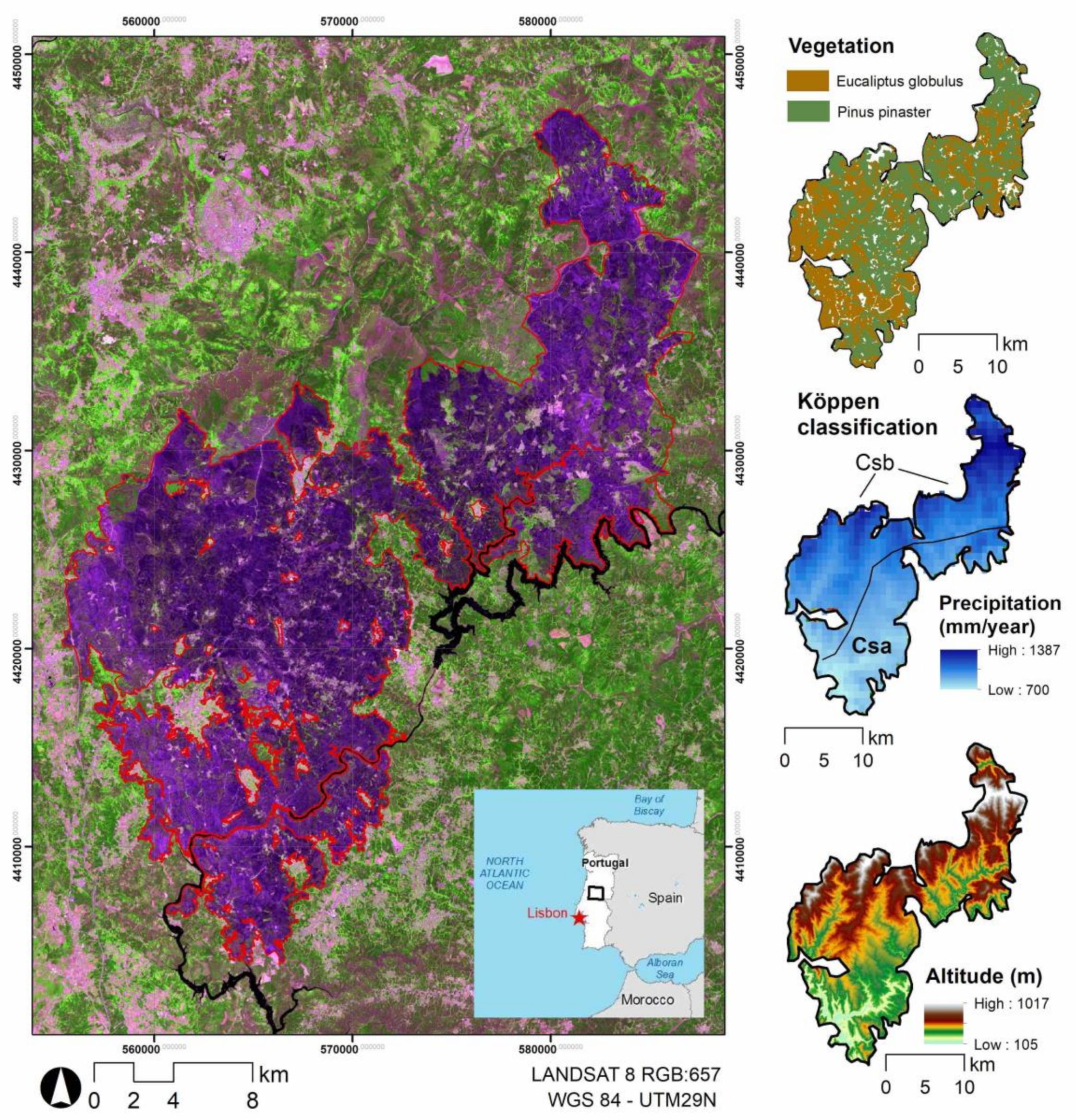
2.1. Study Area
2.2. Materials
3. Methods
3.1. LST Calculation
3.2. LSA Calculation
3.3. ET (METRIC Model)
3.4. Database Construction
3.5. Statistical Analysis
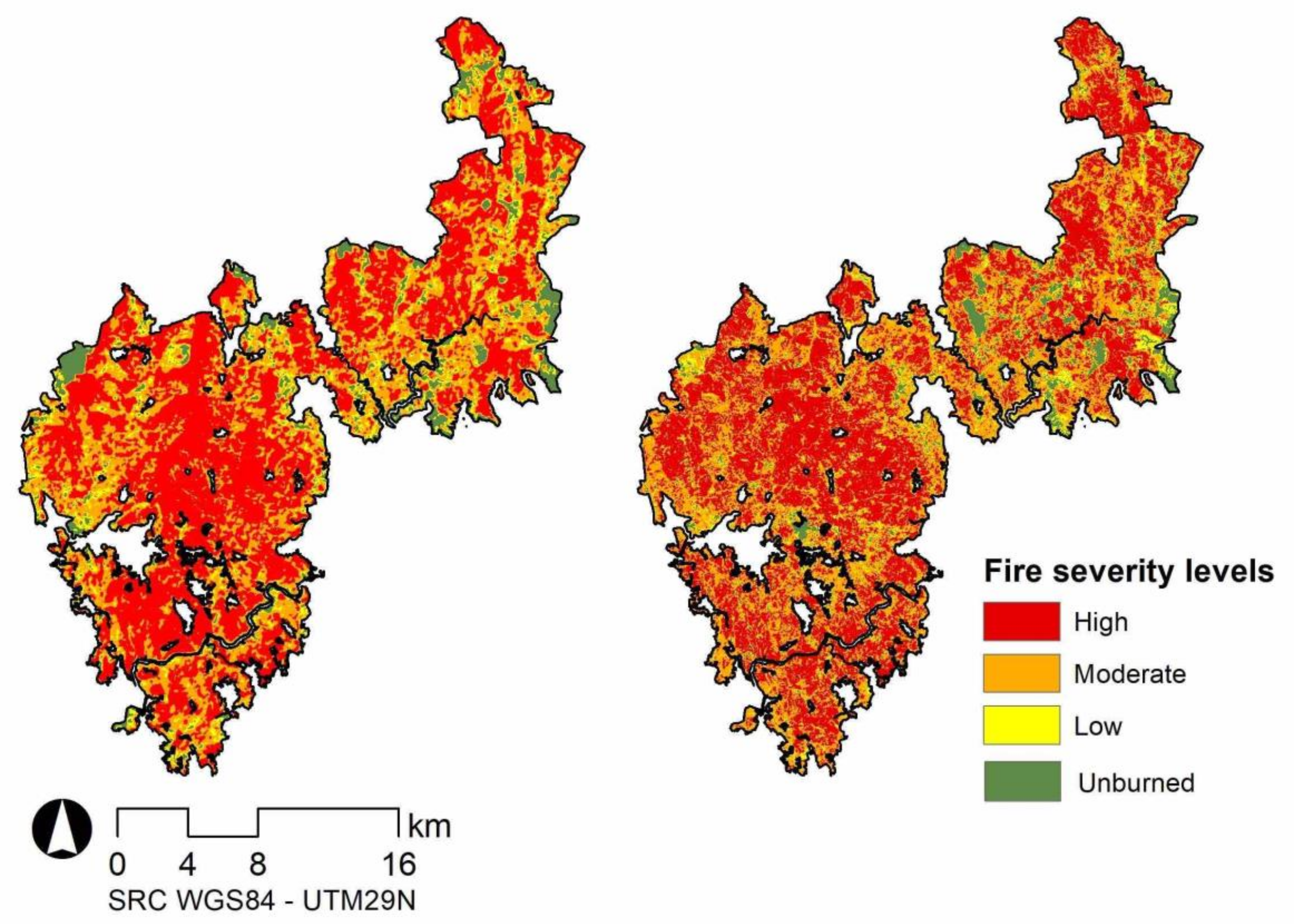
3.6. Burn Severity Mapping
4. Results
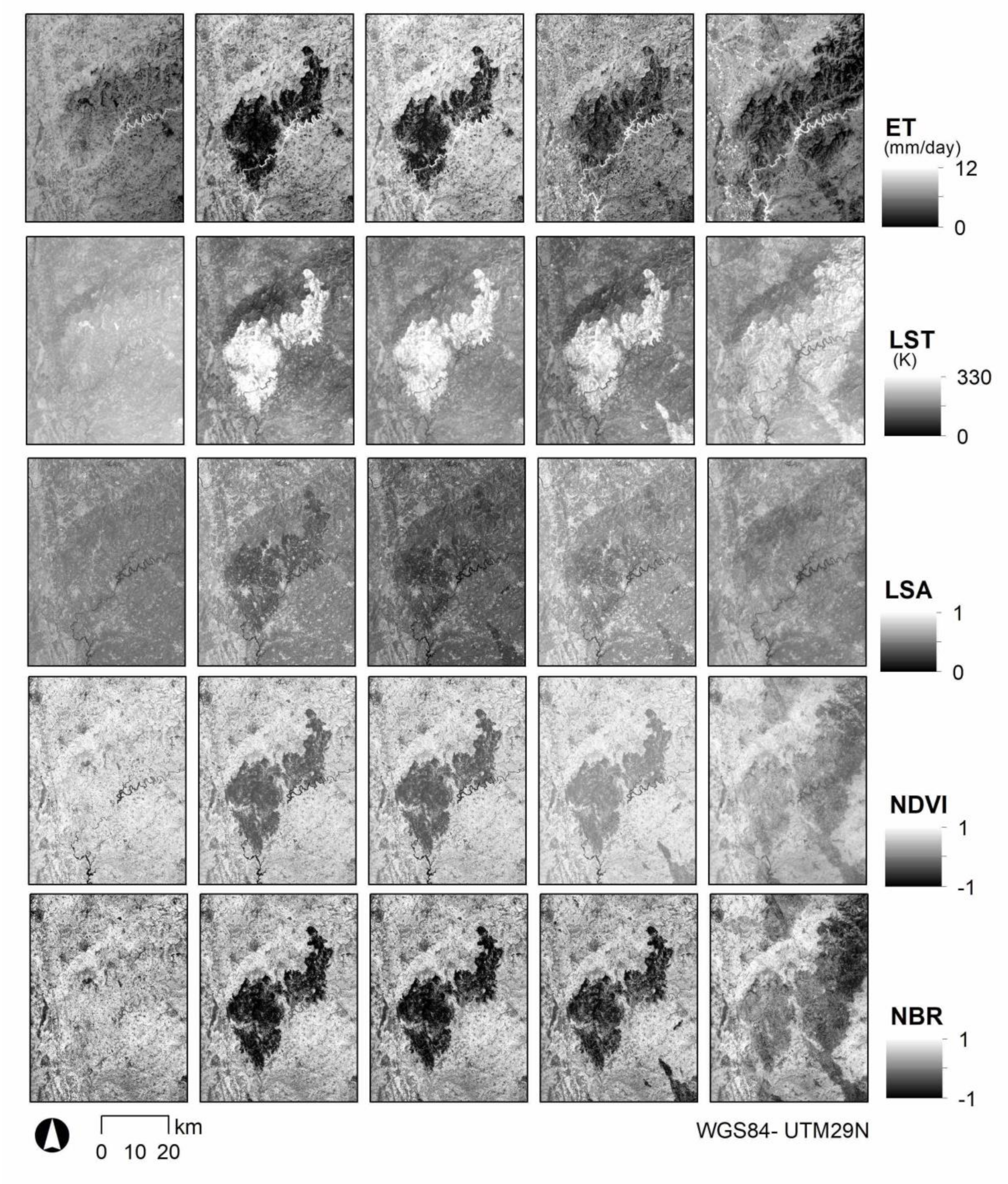
4.1. How Does Fire Modify ET, LST, LSA, NDVI and NBR?
4.2. How Are ET, LST, LSA, NDVI and NBR Post-Fire Images Influenced by Burn Severity and Pre-Fire Factors?
4.3. Is it Possible to Estimate Accurately Burn Severity From the ET, LST and LSA Images?
5. Discussion
5.1. How Does Fire Modify ET, LST, LSA, NDVI and NBR?
5.2. How Are ET, LST, LSA, NDVI and NBR Post-Fire Images Influenced by Burn Severity and Pre-Fire Factors?
5.3. Is it Possible to Accurately Estimate Burn Severity From the ET, LST and LSA Images?
5.4. Final Considerations and Future Work
6. Conclusions
Author Contributions
Funding
Acknowledgments
Conflicts of Interest
References
- Bowman, D.M.J.S.; Balch, J.K.; Artaxo, P.; Bond, W.J.; Carlson, J.M.; Cochrane, M.A.; D’Antonio, C.M.; Defries, R.S.; Doyle, J.C.; Harrison, S.P.; et al. Fire in the earth system. Science 2009, 324, 481–548. [Google Scholar] [CrossRef] [PubMed]
- Scott, A.C.; Bowman, D.M.; Bond, W.J.; Pyne, S.J.; Alexander, M.E. Fire on Earth: An Introduction; John Wiley & Sons: Chichester, UK, 2013. [Google Scholar]
- Leblon, B.; San-Miguel-Ayanz, J.; Bourgeau-Chavez, L.; Kong, M. Remote sensing of wildfires. In Land Surface Remote Sensing: Environment and Risks; Elsevier: Amsterdam, The Netherlands, 2016; pp. 55–95. ISBN 978-1-78548-105-5. [Google Scholar] [CrossRef]
- Meng, R.; Zhao, F. A review for recent advances in burned area and burn severity mapping. In Remote Sensing of Hydrometeorological Hazards; Petropoulos, G.P., Islam, T., Eds.; Taylor & Francis: Abingdon, UK, 2017. [Google Scholar]
- Jain, T.B.; Pilliod, D.; Graham, R.T. Tongue-tied. Confused meanings for common fire terminology can lead to fuels mismanagement. A new framework is needed to clarify and communicate the concepts. Wildfire 2004, 4, 22–26. [Google Scholar]
- Key, C.H.; Benson, N.C. Landscape Assessment (LA) Sampling and Analysis Methods; USDA Forest Service General Technical Reports; Rocky Mountain Research Station: Fort Collins, CO, USA, 2006; RMRS-GTR-164-CD. [Google Scholar]
- Marcos, E.; Villalón, C.; Calvo, L.; Luis-Calabuig, E. Short-term effects of experimental burning on the soil nutrient in the Cantabrian heathlands. Ecol. Eng. 2009, 35, 820–828. [Google Scholar] [CrossRef]
- González-de-Vega, S.; de las Heras, J.; Moya, D. Resilience of Mediterranean terrestrial ecosystems and fire severity in semiarid areas: Responses of Aleppo pine forests in the short, mid and long term. Sci. Total Environ. 2016, 573, 1171–1177. [Google Scholar] [CrossRef]
- Atchley, A.L.; Kinoshita, A.M.; Lopez, S.R.; Trader, L.; Middleton, R. Simulating surface and subsurface water balance changes due to burn severity. Vadose Zone J. 2018, 17, 180099. [Google Scholar] [CrossRef] [Green Version]
- Cardenas, M.B.; Kanarek, M.R. Soil moisture variation and dynamics across a wildfire burn boundary in a loblolly pine (Pinus taeda) forest. J. Hydrol. 2014, 519, 490–502. [Google Scholar] [CrossRef]
- Moody, J.A.; Ebel, B.A. Infiltration and runoff generation processes in fire-affected soils. Hydrol. Process. 2014, 28, 3432–3453. [Google Scholar] [CrossRef]
- Moody, J.A.; Martin, D.A.; Haire, S.L.; Kinner, D.A. Linking runoff response to burn severity after a wildfire. Hydrol. Process. 2008, 22, 2063–2074. [Google Scholar] [CrossRef]
- Clark, K.L.; Skowronski, N.; Gallagher, M.; Renninger, H.; Schäfer, K. Effects of invasive insects and fire on forest energy exchange and evapotranspiration in the New Jersey pinelands. For. Meteorol. 2012, 166, 50–61. [Google Scholar] [CrossRef]
- Lentile, L.; Holden, Z.; Smith, A.; Falkowski, M.; Hudak, A.; Morgan, P.; Lewis, S.; Gessler, P.; Benson, N. Remote sensing techniques to assess active fire characteristics and post-fire effects. Int. J. Wildland Fire 2006, 15, 319–345. [Google Scholar] [CrossRef]
- Rocha, A.V.; Shaver, G.R. Postfire energy exchange in arctic tundra: The importance and climatic implications of burn severity. Glob. Chang. Biol. 2011, 17, 2831–2841. [Google Scholar] [CrossRef]
- Randerson, J.T.; Liu, H.; Flanner, M.G.; Chambers, S.D.; Jin, Y.; Hess, P.G.; Pfister, G.; Mack, M.C.; Treseder, K.K.; Welp, L.R.; et al. The impact of boreal forest fire on climate warming. Science 2006, 314, 1130–1132. [Google Scholar] [CrossRef] [PubMed] [Green Version]
- Sánchez, J.M.; Bisquert, M.; Rubio, E.; Caselles, V. Impact of land cover change induced by a fire event on the surface energy fluxes derived from remote sensing. Remote Sens. 2015, 7, 14899–14915. [Google Scholar] [CrossRef] [Green Version]
- Quintano, C.; Fernández-Manso, A.; Roberts, D.A. Burn severity mapping from Landsat MESMA fraction images and Land Surface Temperature. Remote Sens. Environ. 2017, 190, 83–95. [Google Scholar] [CrossRef]
- Quintano, C.; Fernández-Manso, A.; Calvo, L.; Marcos, E.; Valbuena, L. Land surface temperature as potential indicator of burn severity in forest Mediterranean ecosystems. Int. J. Appl. Earth Obs. 2015, 36, 1–12. [Google Scholar] [CrossRef]
- Veraverbeke, S.; Verstraeten, W.W.; Lhermitte, S.; Van de Kerchove, R.; Goossens, R. Assessment of post-fire changes in land surface temperature and surface albedo, and their relation with fire-burn severity using multi-temporal MODIS imagery. Int. J. Wildland Fire 2012, 21, 243–256. [Google Scholar] [CrossRef] [Green Version]
- Vlassova, L.; Pérez-Cabello, F.; Rodrigues, M.; Montorio, R.; García-Martín, A. Analysis of the relationship between land surface temperature and wildfire severity in a series of Landsat images. Remote Sens. 2014, 6, 6136–6162. [Google Scholar] [CrossRef] [Green Version]
- Beringer, J.; Hutley, L.; Tapper, N.; Coutts, A.; Kerley, A.; O’Grady, A. Fire impacts on surface heat, moisture and carbon fluxes from a tropical savanna in northern Australia. Int. J. Wildland Fire 2003, 12, 333–340. [Google Scholar] [CrossRef]
- Quintano, C.; Fernández-Manso, A.; Fernández-García, V.; Marcos, E.; Calvo, L. Changes on albedo after a large forest fire in Mediterranean ecosystems. In Proceedings of the Remote Sensing and Modeling of Ecosystems for Sustainability XII (SPIE 9610), San Diego, CA, USA, 11–12 August 2015. [Google Scholar] [CrossRef]
- Quintano, C.; Fernandez-Manso, A.; Marcos, E.; Calvo, L. Burn severity and post-fire land surface albedo relationship in Mediterranean forest ecosystems. Remote Sens. 2019, 11, 2309. [Google Scholar] [CrossRef] [Green Version]
- Liu, Z.; Ballantyne, A.P.; Cooper, L.A. Increases in land surface temperature in response to fire in Siberian boreal forests and their attribution to biophysical processes. Geophys. Res. Lett. 2018, 45, 6485–6494. [Google Scholar] [CrossRef]
- Ellison, D.; Morris, C.E.; Locatelli, B.; Sheil, D.; Cohen, J.; Murdiyarso, D.; Gutierrez, V.; van Noordwijkl, M.; Creed, I.F.; Pokorny, J.; et al. Trees, forests and water: Cool insights for a hot world. Sci. Tech. 2017, 43, 51–61. [Google Scholar] [CrossRef]
- Amiro, B.D.; MacPherson, J.I.; Desjardins, R.L. BOREAS flight measurements of forest-fire effects on carbon dioxide and energy fluxes. Agric. For. Meteorol. 1999, 96, 199–208. [Google Scholar] [CrossRef]
- Dintwe, K.; Okin, G.S.; Xue, Y. Fire-induced albedo change and surface radiative forcing in sub-Saharan Africa savanna ecosystems: Implications for the energy balance. J. Geophys. Res. Atmos. 2017, 122, 6186–6201. [Google Scholar] [CrossRef] [Green Version]
- Alkama, R.; Cescatti, A. Biophysical climate impacts of recent changes in global forest cover. Science 2016, 351, 600–604. [Google Scholar] [CrossRef] [PubMed] [Green Version]
- Liu, Z.; Ballantyne, A.P.; Cooper, L.A. Biophysical feedback of global forest fires on surface temperature. Nat. Commun. 2019, 10, 214. [Google Scholar] [CrossRef] [Green Version]
- Benmechet, A.; Abdellaoui, A.; Hamou, A. A comparative study of land surface temperature retrieval methods from remote sensing data. Can. J. Remote Sens. 2013, 39, 59–73. [Google Scholar] [CrossRef]
- Li, Z.-L.; Tang, B.-H.; Wu, H.; Ren, H.; Yan, G.; Wan, Z.; Trigo, I.F.; Sobrino, J.A. Satellite-derived land surface temperature: Current status and perspectives. Remote Sens. Environ. 2013, 131, 14–37. [Google Scholar] [CrossRef] [Green Version]
- Coakley, J.A., Jr. Reflectance and albedo, surface. In Encyclopedia of the Atmosphere; Holton, J.R., Curry, J.A., Eds.; Academic Press: Cambridge, CA, USA, 2002; pp. 1914–1923. [Google Scholar]
- Liang, S.; Shuey, C.J.; Russ, A.L.; Fang, H.; Chen, M.; Walthall, C.L.; Daughtry, C.S.T.; Hunt, R., Jr. Narrowband to broadband conversions of land surface albedo: II. Validation. Remote Sens. Environ. 2002, 84, 25–41. [Google Scholar] [CrossRef]
- Dore, S.; Kolb, T.E.; Montes-Helu, M.; Eckert, S.E.; Sullivan, B.W.; Hungate, B.A.; Kaye, J.P.; Hart, S.C.; Koch, G.W.; Finkral, A. Carbon and water fluxes from ponderosa pine forests disturbed by wildfire and thinning. Ecol. Appl. 2010, 20, 663–683. [Google Scholar] [CrossRef]
- Montes-Helu, M.C.; Kolb, T.; Dore, S.; Sullivan, B.; Hart, S.C.; Koch, G.; Hungate, B.A. Persistent effects of fire-induced vegetation change on energy partitioning and evapotranspiration in ponderosa pine forests. Agric. For. Meteorol. 2009, 149, 491–500. [Google Scholar] [CrossRef]
- Häusler, M.; Nunes, J.P.; Soares, P.; Sánchez, J.M.; Silva, J.M.N.; Warneke, T.; Keizer, J.J.; Pereira, J.M.C. Assessment of the indirect impact of wildfire (severity) on actual evapotranspiration in eucalyptus forest based on the surface energy balance estimated from remote-sensing techniques. Int. J. Remote Sens. 2018, 39, 6499–6524. [Google Scholar] [CrossRef]
- Van der Tol, C.; Norberto-Parodi, G. Guidelines for remote sensing of evapotranspiration. In Evapotranspiration—Remote Sensing and Modeling; Irmak, A., Ed.; InTech: Croatia, Balkans, 2011; pp. 227–250. [Google Scholar]
- Allen, R.G.; Tasumi, M.; Trezza, R. Satellite-based energy balance for mapping evapotranspiration with internalized calibration (METRIC)-Model. J. Irrig. Drain. Eng. 2007, 133, 380–394. [Google Scholar] [CrossRef]
- De la Fuente-Sáiz, D.; Ortega-Farí, S.; Fonseca, D.; Ortega-Salazar, S.; Kilic, A.; Allen, R. Calibration of METRIC model to estimate energy balance over a drip-irrigated apple orchard. Remote Sens. 2017, 9, 670. [Google Scholar] [CrossRef] [Green Version]
- Foolad, F.; Blankenau, P.; Kilic, A.; Allen, R.G.; Huntington, J.L.; Erickson, T.A.; Ozturk, D.; Morton, C.G.; Ortega, S.; Ratcliffe, I.; et al. Comparison of the automatically calibrated Google Evapotranspiration Application—EEFlux and the manually calibrated METRIC application. Preprints 2018. [Google Scholar] [CrossRef]
- Allen, R.G.; Burnett, B.; Kramber, W.; Huntington, J.; Kjaersgaard, J.; Kilic, A.; Kelly, C.; Trezza, R. Automated calibration of the METRIC-landsat evapotranspiration process. J. Am. Water Resour. Assoc. 2013, 49, 563–576. [Google Scholar] [CrossRef]
- Morton, C.G.; Huntington, J.L.; Pohll, G.M.; Allen, R.G.; McGwire, K.C.; Bassett, S.D. Assessing calibration uncertainty and automation for estimating evapotranspiration from agricultural areas using METRIC. J. Am. Water Resour. Assoc. 2013, 49, 549–562. [Google Scholar] [CrossRef]
- Allen, R.; Morton, C.; Kamble, B.; Kilic, A.; Huntington, J.; Thau, D.; Gorelick, N.; Erickson, T.; Moore, R.; Trezza, R.; et al. EEFlux: A Landsat-based Evapotranspiration mapping tool on the Google Earth Engine. In Proceedings of the 2015 Irrigation Symposium: Emerging Technologies for Sustainable Irrigation, Long Beach, CA, USA, 10–12 November 2015; ASABE: St. Joseph, MI, USA Publication No. 701P0415; Paper Number 43511. [Google Scholar]
- Fisher, J.B.; Hook, R.; Allen, R.G.; Anderson, M.C.; French, A.N.; Hain, C.R.; Hulley, G.; Wood, E.F. The ECOsystem Spaceborne Thermal Radiometer Experiment on Space Station (ECOSTRESS): Science motivation. In Proceedings of the American Geophysical Union Fall Meeting, San Francisco, CA, USA, 15–19 December 2014. Abstract id. H31J-07. [Google Scholar]
- Fisher, J.B.; Melton, F.; Middleton, E.; Hain, C.; Anderson, M.; Allen, R.; McCabe, M.F.; Hook, S.; Baldocchi, D.; Townsend, P.A.; et al. The future of evapotranspiration: Global requirements for ecosystem functioning, carbon and climate feedbacks, agricultural management, and water resources. Water Resour. Res. 2017, 53, 2618–2626. [Google Scholar] [CrossRef]
- Baldocchi, D.; Falge, E.; Gu, L.; Olson, R.; Hollinger, D.; Running, S.; Anthoni, P.; Bernhofer, C.; Davis, K.; Evans, R.; et al. FLUXNET: A new tool to study the temporal and spatial variability of ecosystem-scale carbon dioxide, water vapor, and energy flux densities. Bull. Am. Meteorol. Soc. 2001, 82, 2415–2434. [Google Scholar] [CrossRef]
- Cabral, A.I.R.; Silva, S.; Silva, P.C.; Vanneschi, L.; Vasconcelos, M.J. Burned area estimations derived from Landsat ETM+ and OLI data: Comparing genetic programming with maximum likelihood and classification and regression Trees. ISPRS J. Photogramm. Remote Sens. 2018, 142, 94–105. [Google Scholar] [CrossRef]
- Chen, G.; Metz, M.R.; Rizzo, D.M.; Dillon, W.W.; Meentemeyer, R.K. Object-based assessment of burn severity in diseased forests using high-spatial and high-spectral resolution MASTER airborne imagery. ISPRS J. Photogramm. Remote Sens. 2015, 102, 38–47. [Google Scholar] [CrossRef] [Green Version]
- Fernández-Manso, A.; Quintano, C.; Roberts, D.A. Burn severity analysis in Mediterranean forests using maximum entropy model trained with EO-1 Hyperion and LiDAR data. ISPRS J. Photogramm. Remote Sens. 2019, 155, 102–118. [Google Scholar] [CrossRef]
- Veraverbeke, S.; Dennison, P.; Gitas, I.; Hulley, G.; Kalashnikova, O.; Katagis, T.; Kuai, L.; Meng, R.; Roberts, D.; Stavros, N. Hyperspectral remote sensing of fire: State-of-the-art and future perspectives. Remote Sens. Environ. 2018, 216, 105–121. [Google Scholar] [CrossRef]
- Franco, M.G.; Mundo, I.A.; Veblen, T.T. Field-validated burn-severity mapping in north Patagonian forests. Remote Sens. 2020, 12, 214. [Google Scholar] [CrossRef] [Green Version]
- Fornacca, D.; Ren, G.; Xiao, W. Evaluating the best spectral indices for the detection of burn scars at several post-fire dates in a mountainous region of Northwest Yunnan, China. Remote Sens. 2018, 10, 1196. [Google Scholar] [CrossRef] [Green Version]
- Arnett, J.T.T.R.; Coops, N.C.; Daniels, L.D.; Falls, R.W. Detecting forest damage after a low-severity fire using remote sensing at multiple scales. Int. J. Appl. Earth Obs. 2015, 35, 239–246. [Google Scholar] [CrossRef]
- Fernández-Manso, A.; Fernandez-Manso, O.; Quintano, C. SENTINEL-2A red-edge spectral indices suitability for discriminating burn severity. Int. J. Appl. Earth Obs. 2016, 50, 170–175. [Google Scholar] [CrossRef]
- Lu, B.; He, Y.; Tong, A. Evaluation of spectral indices for estimating burn severity in semiarid grasslands. Int. J. Wildland Fire 2015, 25, 147–157. [Google Scholar] [CrossRef]
- Quintano, C.; Fernández-Manso, A.; Fernández-Manso, O. Combination of Landsat and Sentinel-2 MSI data for initial assessing of burn severity. Int. J. Appl. Earth Obs. 2018, 64, 221–225. [Google Scholar] [CrossRef]
- Tanase, M.; de la Riva, J.; Pérez-Cabello, F. Estimating burn severity in Aragón pine forest using optical based indices. Can. J. Forest Res. 2011, 41, 863–872. [Google Scholar] [CrossRef]
- Szpakowski, D.M.; Jensen, J.L.R. A review of the applications of remote sensing in fire ecology. Remote Sens. 2019, 11, 2638. [Google Scholar] [CrossRef] [Green Version]
- Soverel, N.O.; Perrakis, D.D.B.; Coops, N.C. Estimating burn severity from Landsat dNBR and RdNBR indices across western Canada. Remote Sens. Environ. 2010, 114, 1896–1909. [Google Scholar] [CrossRef]
- Stambaugh, M.C.; Hammer, L.D.; Godfrey, R. Performance of burn-severity metrics and classification in oak woodlands and grasslands. Remote Sens. 2015, 7, 10501–10522. [Google Scholar] [CrossRef] [Green Version]
- Zhu, Z.; Key, C.; Ohlen, D.; Benson, N. Evaluate Sensitivities of Burn-Severity Mapping Algorithms for Different Ecosystems and Fire Histories in the United States. In Evaluate Sensitivities of Burn-Severity Mapping Algorithms for Different Ecosystems and Fire Histories in the United States; Final Report to the Joint Fire Science Program; USGS (United States Geological Survey): Reston, VA, USA; National Park Service Fire Management Program Center: Boise, ID, USA, 2006; Project: JFSP 01-1-4-12. [Google Scholar]
- Carvajal-Ramírez, F.; da Silva, J.R.M.; Agüera-Vega, F.; Martínez-Carricondo, P.; Serrano, J.; Moral, F.J. Evaluation of fire severity indices based on pre- and post-fire multispectral imagery sensed from UAV Remote Sens. Remote Sens. 2019, 11, 993. [Google Scholar] [CrossRef] [Green Version]
- Harvey, B.J.; Donato, D.C.; Turner, M.G. Drivers and trends in landscape patterns of stand-replacing fire in forests of the US Northern Rocky Mountains (1984–2010). Landsc. Ecol. 2016, 31, 2367–2383. [Google Scholar] [CrossRef]
- Morgan, P.; Keane, R.E.; Dillon, G.K.; Jain, T.B.; Hudak, A.T.; Karau, E.C.; Sikkink, P.G.; Holden, Z.A.; Strand, E.K. Challenges of assessing fire and burn severity using field measures, remote sensing and modelling. Int. J. Wildland Fire 2014, 23, 1045–1060. [Google Scholar] [CrossRef] [Green Version]
- Lentille, L.B.; Smith, A.M.S.; Hudak, A.T.; Morgan, P.; Bobbitt, M.J.; Lewis, S.A.; Robichaud, P.R. Remote sensing for prediction of 1-year post-fire ecosystem condition. Int. J. Wildland Fire 2009, 18, 594–608. [Google Scholar] [CrossRef] [Green Version]
- San-Miguel-Ayanz, J.; Durrant, T.; Boca, R.; Libertà, G.; Branco, A.; de Rigo, D.; Ferrari, D.; Maianti, P.; Vivancos, T.A.; Costa, H.; et al. Forest Fires in Europe, Middle East and North Africa 2017; European Comission, Joint Research Centre: Ispra, Italy, 2018; ISBN 978-92-79-92831-4. [Google Scholar] [CrossRef]
- Ribeiro, L.M.; Rodrigues, A.; Lucas, D.; Viegas, D.X. The large fire of Pedrógão Grande (Portugal) and its impact on structures. Adv. For. Fire Res. 2018, 852–858. [Google Scholar] [CrossRef] [Green Version]
- ADAI/LAETA. O Complexo de Incêndios de Pedrógão Grande e Concelhos Limítrofes, Iniciado a 17 de Junho de 2017; Universidade de Coimbra Official Report; Universidade de Coimbra: Coimbra, Portugal, 2017. (In Portuguese) [Google Scholar]
- Pinto, P.; Silva, A. Advances in Forest Fire Research; Viegas, D.X., Ed. ADAI/CEIF University of Coimbra, Portugal; 2018; pp. In Atmospheric Flow and a Large Fire Interaction: The Unusual Case of Pedrogão Grande, Portugal (17 June 2017); Viegas, D.X., Ed.; ADAI/CEIF; University of Coimbra: Coimbra, Portugal, 2018; pp. 922–932. [Google Scholar] [CrossRef] [Green Version]
- CTI, Análise e Apuramento Dos Factos Relativos Aos Incêndios Que Ocorreram Em Pedrogão Grande, Castanheira de Pêra, Ansião, Alvaiázere, Figueiró dos Vinhos, Arganil, Góis, Penela, Pampilhosa da Serra, Oleiros e Sertã, Entre 17 e 24 de Junho de 2017; Assembleia da República: Lisboa, Portugal, 2017.
- Köppen, W. Das Geographische System der Klimate, 1–44; Gebrüder Borntraeger: Berlin, Germany, 1936. [Google Scholar]
- DGT. Especificações Técnicas da Carta de Uso e Ocupação do Solo de Portugal Continental Para 1995, 2007, 2010 e 2015; Relatório Técnico; Direção-Geral do Território: Lisboa, Portugal, 2018. [Google Scholar]
- Peel, M.C.; Finlayson, B.L.; McMahon, T.A. Updated world map of the Köppen-Geiger climate classification. Hydrol. Earth Syst. Sci. 2007, 11, 1633–1644. [Google Scholar] [CrossRef] [Green Version]
- Quintano, C.; Fernández-Manso, A.; Calvo, L.; Roberts, D.A. Vegetation and soil fire damage analysis based on species distribution modeling trained with multispectral satellite data. Remote Sens. 2019, 11, 1832. [Google Scholar] [CrossRef] [Green Version]
- Fernández-García, V.; Quintano, C.; Taboada, A.; Marcos, E.; Calvo, L.; Fernández-Manso, A. Remote sensing applied to the study of fire regime attributes and their influence on post-fire greenness recovery in pine ecosystems. Remote Sens. 2018, 10, 733. [Google Scholar] [CrossRef] [Green Version]
- Yu, X.; Guo, X.; Wu, Z. Land surface temperature retrieval from Landsat 8 TIRS—Comparison between radiative transfer equation-based method, split window algorithm and single channel method. Remote Sens. 2014, 6, 9829–9852. [Google Scholar] [CrossRef] [Green Version]
- R Core Team. R: A Language and Environment for Statistical Computing, URL. Available online: http://www.R-project.org (accessed on 23 October 2019).
- Sobrino, J.A.; Jiménez-Muñoz, J.C.; Sòria, G.; Romaguera, M.; Guanter, L.; Moreno, J.; Plaza, A.; Martínez, P. Land surface emissivity retrieval from different VNIR and TIR sensors. IEEE T. Geosci. Remote 2008, 48, 316–327. [Google Scholar] [CrossRef]
- Liang, S. Narrowband to broadband conversions of land surface albedo. I Algorithms. Remote Sens. Environ. 2000, 76, 213–238. [Google Scholar] [CrossRef]
- Irmak, A.; Allen, R.G.; Kjaersgaard, J.; Huntington, J.; Kamble, B.; Trezza, R.; Ratcliffe, I. Operational remote sensing of ET and challenges. In Evapotranspiration—Remote Sensing and Modeling; Irmak, A., Ed.; InTech: Rijeka, Croatia, 2011; p. 526. [Google Scholar]
- López-García, M.J.; Caselles, V. Mapping burns and natural reforestation using Thematic Mapper data. Geocarto Int. 1991, 1, 31–37. [Google Scholar] [CrossRef]
- Tucker, C.J. Red and photographic infrared linear combinations formonitoring vegetation. Remote Sens. Environ. 1979, 8, 127–150. [Google Scholar] [CrossRef] [Green Version]
- Congalton, R.G.; Green, K. Assessing the Accuracy of Remotely Sensed Data. Principles and Practices, 2nd ed.; CRC Press: Boca Ratón, FL, USA, 2009. [Google Scholar]
- Weatherspoon, C.P.; Skinner, C.N. An assessment of factors associated with damage to tree crowns from the 1987 wildfires in northern California. For. Sci. 1995, 41, 430–451. [Google Scholar]
- Godwin, D.R.; Kobziar, L.N. Comparison of burn severities of consecutive large-scale fires in Florida sand pine scrub using satellite imagery analysis. Fire Ecol. 2011, 7, 99–113. [Google Scholar] [CrossRef]
- Miler, J.D.; Thode, A.E. Quantifying burn severity in a heterogeneous landscape with a relative version of the delta Normalized Burn Ratio (dNBR). Remote Sens. Environ. 2007, 109, 66–80. [Google Scholar] [CrossRef]
- Botella-Martínez, M.A.; Fernández-Manso, A. Study of post-fire severity in the Valencia region comparing the NBR, RdNBR and RBR indexes derived from Landsat 8 images. Span. J. Remote Sens. Rev. Asoc. Española Teledetección 2017, 49, 33–47. [Google Scholar]
- Poon, P.K.; Kinoshita, A.M. Spatial and temporal evapotranspiration trends after wildfire in semi-arid landscapes. J. Hydrol. 2018, 559, 71–83. [Google Scholar] [CrossRef]
- Li, X.; Zhang, H.; Yang, G.; Ding, Y.; Zhao, J. Post-Fire vegetation succession and surface energy fluxes derived from remote sensing. Remote Sens. 2018, 10, 1000. [Google Scholar] [CrossRef] [Green Version]
- Roche, J.W.; Goulden, M.L.; Bales, R.C. Estimating evapotranspiration change due to forest treatment and fire at the basin scale in the Sierra Nevada, California. Ecohydrology 2018, 11, e1978. [Google Scholar] [CrossRef]
- Nolan, R.H.; Lane, P.N.J.; Benyon, R.G.; Bradstock, R.A.; Mitchell, P.J. Changes in evapotranspiration following wildfire in resprouting eucalypt forests. Ecohydrology 2014, 7, 1363–1377. [Google Scholar] [CrossRef]
- Huang, S.; Jin, S.; Dahal, D.; Chen, X.; Young, C.; Liu, H.; Liu, S. Reconstructing satellite images to quantify spatially explicit land surface change caused by fires and succession: A demonstration in the Yukon River Basin of interior Alaska. ISPRS J. Photogramm. Remote Sens. 2013, 79, 94–105. [Google Scholar] [CrossRef]
- Lambin, E.; Goyvaerts, K.; Petit, C. Remotely-sensed indicators of burn-ing efficiency of savannah and forest fires. Int. J. Remote Sens. 2003, 24, 3105–3118. [Google Scholar] [CrossRef]
- Mölders, N.; Kramm, G. Influence of wildfire induced land-cover changes on clouds and precipitation in interior Alaska—A case of study. Atmos. Res. 2007, 82, 142–168. [Google Scholar] [CrossRef]
- Veraverbeke, S.; Van de Kerchove, R.; Verstraeten, W.; Lhermitte, S.; Goossens, R. Fire-induced changes in vegetation, albedo and land surface temperature assessed with MODIS. In Proceedings of the EARSeL Symposium 2010 Remote Sensing for Science, Education, and Natural and Cultural Heritage, Paris, France, 31 May–1 June 2010; University of Oldenburg: Oldenburg, Germany, 2010; pp. 431–438. [Google Scholar]
- Wendt, C.; Beringer, J.; Tapper, N.; Hutley, L. Local boundary-layer development over burnt and unburnt tropical savanna: An observational study. Bound. Layer Meteorol. 2007, 124, 291–304. [Google Scholar] [CrossRef]
- Amiro, B.D.; Orchansky, A.L.; Barr, A.G.; Black, T.A.; Chambers, S.D.; Chapin, F.S., III; Goulden, M.L.; Litvak, M.; Liu, H.P.; McCaughey, J.H.; et al. The effect of post-fire stand age on the boreal forest energy balance. Agric. For. Meteorol. 2006, 140, 41–50. [Google Scholar] [CrossRef] [Green Version]
- Gatebe, C.K.; Ichoku, C.M.; Poudyal, R.; Román, M.O.; Wilcox, E. Surface albedo darkening from wildfires in northern sub-Saharan Africa. Environ. Res. Lett. 2014, 9, 065003. [Google Scholar] [CrossRef] [Green Version]
- Tessler, N.; Wittenberg, L.; Greenbaum, N. Vegetation cover and species richness after recurrent forest fires in the Eastern Mediterranean Ecosystem of Mount Carmel, Israel. Sci. Total Environ. 2016, 572, 1395–1402. [Google Scholar] [CrossRef]
- Bastos, A.; Gouveia, C.M.; DaCamara, C.C.; Trigo, R.M. Modelling post-fire vegetation recovery in 899 Portugal. Biogeo Sci. 2011, 8, 3593–3607. [Google Scholar] [CrossRef] [Green Version]
- Whittock, S.P.; Apiolaza, L.A.; Kelly, C.M.; Potts, B.M. Genetic control of coppice and lignotuber development in Eucalyptus globulus. Aust. J. Bot. 2003, 51, 57–68. [Google Scholar] [CrossRef]
- Herranz, J.M.; Martínez-Sánchez, J.J.; Marín, A.; Ferrandis, P. Post-fire regeneration of Pinus halepensis Miller in a semi-arid area in Albacete province (south-eastern Spain). Ecoscience 1997, 4, 86–90. [Google Scholar] [CrossRef]
- Kontoes, C.C.; Poilve, H.; Florsch, G.; Keramitsoglou, I.; Paralikidis, S. A comparative analysis of a fixed thresholding vs. A classification tree approach for operational burn scar detection and mapping. Int. J. Appl. Earth Obs. 2009, 11, 299–316. [Google Scholar] [CrossRef]
- Pereira, J.M.C.; Sa, A.C.L.; Sousa, A.M.O.; Martín, M.P.; Chuvieco, E. Regional-scale burnt area mapping in Southern Europe using NOAA-AVHRR 1 km data. In Remote Sensing of Large Wildfires in the European Mediterranean Basin; Chuvieco, E., Ed.; Springer: Berlin, Germany, 1999; pp. 139–155. [Google Scholar]
- Martín, M.P.; Gómez, I.; Chuvieco, E. Performance of a burned-area index (BAIM) for mapping Mediterranean burned scars from MODIS data. In Proceedings of the 5th International Workshop on Remote Sensing and GIS Applications to Forest Fire Management: Fire Effects Assessment, Zaragoza, Spain, 16–18 June 2005; Universidad de Zaragoza: Zaragoza, Spain, 2005. [Google Scholar]
- Salvador, R.; Valeriano, J.; Pons, X.; Díaz-Delgado, R. A semiautomatic methodology to detect fire scars in shrubs and evergreen forest with Landsat MSS time series. Int. J. Remote Sens. 2000, 21, 655–671. [Google Scholar] [CrossRef] [Green Version]
- Quintano, C.; Fernández-Manso, A.; Roberts, D.A. Multiple endmember spectral mixture analysis (MESMA) to map burn severity levels from Landsat images in Mediterranean countries. Remote Sens. Environ. 2013, 136, 76–88. [Google Scholar] [CrossRef]
- Tane, Z.; Roberts, D.; Veraverbeke, S.; Casas, A.; Ramirez, C.; Ustin, S. Evaluating endmember and band selection techniques for multiple endmember spectral mixture analysis using post-fire imaging spectroscopy. Remote Sens. 2018, 10, 389. [Google Scholar] [CrossRef] [Green Version]
- Veraverbeke, S.; Hook, S.J. Evaluating spectral indices and spectral mixture analysis for assessing fire severity, combustion completeness and carbon emissions. Int. J. Wildland Fire 2013, 22, 707–720. [Google Scholar] [CrossRef]
- Rogers, B.M.; Soja, A.J.; Goulden, M.L.; Randerson, J.T. Influence of tree species on continental differences in boreal fires and climate feedbacks. Nat. Geosci. 2015, 8, 228–234. [Google Scholar] [CrossRef]
- Goulden, M.L.; Bales, R.C. Mountain runoff vulnerability to increased evapotranspiration with vegetation expansion. Proc. Natl. Acad. Sci. USA 2014, 111, 14071–14075. [Google Scholar] [CrossRef] [Green Version]
- Venâncio, P. Open Source, Open Data e Citizen Science contributos para a Avaliação da Catástrofe de Pedrógão Grande e Góis. In SASIG 2017. In Proceedings of the Encontro Nacional de Software Aberto para Sistemas de Informação Geográfica, Porto, Portugal, 20–22 November 2017. [Google Scholar]
- Cocke, A.E.; Fulé, P.Z.; Crouse, J.E. Comparison of burn severity assessments using differenced normalized burn ratio and ground data. Int. J. Wildland Fire 2005, 14, 189–198. [Google Scholar] [CrossRef] [Green Version]
- Cansler, C.A.; McKenzie, D. How robust are burn severity indices when applied in a new region? Evaluation of alternate field-based and remote-sensing methods. Remote Sens. 2012, 4, 456–483. [Google Scholar] [CrossRef] [Green Version]
- Amos, C.; Petropoulos, G.P.; Ferentinos, K.P. Determining the use of Sentinel-2A MSI for wildfire burning & severity detection. Int. J. Remote Sens. 2019, 40, 905–930. [Google Scholar] [CrossRef]
- Tran, B.N.; Tanase, M.A.; Bennett, L.T.; Aponte, C. Evaluation of spectral indices for assessing fire severity in australian temperate forests. Remote Sens. 2018, 10, 1680. [Google Scholar] [CrossRef] [Green Version]
- Parks, S.A.; Holsinger, L.M.; Panunto, M.H.; Jolly, W.M.; Dobrowski, S.Z.; Dillon, G.K. High-severity fire: Evaluating its key drivers and mapping its probability across western US forests. Environ. Res. Lett 2018, 13, 044037. [Google Scholar] [CrossRef]
- Harvey, B.J.; Andrus, R.A.; Anderson, S.C. Incorporating biophysical gradients and uncertainty into burn severity maps in a temperate fire-prone forested region. Ecosphere 2019, 10. [Google Scholar] [CrossRef] [Green Version]
- Ewers, B.E.; Gower, S.T.; Bond-Lamberty, B.; Wang, C. Effects of stand age and tree species composition on transpiration and canopy conductance of boreal forest stands. Plant Cell Environ. 2005, 28, 660–678. [Google Scholar] [CrossRef]
- Valeo, C.; Beaty, K.; Hesslein, R. Influence of forest fires on climate change studies in the central boreal forest of Canada. J. Hydrol. 2003, 280, 91–104. [Google Scholar] [CrossRef]
- Bond-Lamberty, B.; Peckham, S.D.; Gower, S.T.; Ewers, B.E. Effects of fire on regional evapotranspiration in the central Canadian boreal forest. Glob. Chang. Biol. 2009, 15, 1242–1254. [Google Scholar] [CrossRef] [Green Version]
- Cai, X.; Riley, W.J.; Zhu, Q.; Tang, J.; Zeng, Z.; Bisht, G.; Randerson, J.T. Improving representation of deforestation effects on evapotranspiration in the E3SM land model. J. Adv. Model. Earth Syst. 2019. [Google Scholar] [CrossRef] [Green Version]
- Nolan, R.H.; Lane, P.N.J.; Benyon, R.G.; Bradstock, R.A.; Mitchell, P.J. Trends in evapotranspiration and streamflow following wildfire in resprouting eucalypt forests. J. Hydrol. 2015, 524, 614–624. [Google Scholar] [CrossRef]
- García-Llamas, P.; Suárez-Seoane, S.; Taboada, A.; Fernández-García, V.; Fernández-Guisuraga, J.M.; Fernández-Manso, A.; Quintano, C.; Marcos, E.; Calvo, L. Assessment of the influence of biophysical properties related to fuel conditions on fire severity using remote sensing techniques: A case study on a large fire in NW Spain. Int. J. Wildland Fire 2019, 28, 512–520. [Google Scholar] [CrossRef]
- Ha, W.; Kolb, T.E.; Springer, A.E.; Dore, S.; O′Donnell, F.C.; Martínez, R.; López, S.; Koch, G.W. Evapotranspiration comparisons between eddy covariance measurements and meteorological and remote-sensing-based models in disturbed ponderosa pine forests. Ecohydrology 2014, 8, 1335. [Google Scholar] [CrossRef]
- Qazi, N.Q.; Bruijnzeel, L.A.; Rai, S.P.; Ghimire, C.P. Impact of forest degradation on streamflow regime and runoff response to rainfall in the Garhwal Himalaya, Northwest India. Hydrolog. Sci. J. 2017, 62, 1114–1130. [Google Scholar] [CrossRef]
- Pimentel, R.; Arheimer, B. Wildfire impact on Boreal hydrology: Empirical study of the Västmanland fire 2014 (Sweden). Hydrol. Earth Syst. Sci. Discuss. 2018, 1–26. [Google Scholar] [CrossRef]
- Van der Ent, R.J.; Wang-Erlandsson, L.; Keys, P.W.; Savenije, H.H.G. Contrasting roles of interception and transpiration in the hydrological cycle—Part 2: Moisture recycling. Earth Syst. Dynam. 2014, 5, 471–489. [Google Scholar] [CrossRef] [Green Version]
- Jeffery, M.L.; Yanites, B.J.; Poulsen, C.J.; Ehlers, T.A. Vegetation-precipitation controls on Central Andean topography. J. Geophys. Res. Earth 2014, 119, 1354–1375. [Google Scholar] [CrossRef] [Green Version]
- Cerda, A.; Robichaud, P.R. Fire Effects on Soils and Restoration Strategies; CRC Press: Boca Ratón, FL, USA, 2009. [Google Scholar]
- Smith, H.G.; Sheridan, G.J.; Lane, P.N.J.; Nyman, P.; Haydon, S. Wildfire effects on water quality in forest catchments: A review with implications for water supply. J. Hydrol. 2011, 396, 170–192. [Google Scholar] [CrossRef]


| 06/15/17 | 07/01/17 | 08/02/17 | 09/19/17 | 08/05/18 | |||||||
|---|---|---|---|---|---|---|---|---|---|---|---|
| μ | σ | μ | σ | μ | σ | μ | σ | μ | σ | ||
| ET (mm/day) | Burned | - | - | 1.62 | 1.62 | 1.62 | 0.95 | 1.52 | 0.98 | 1.76 | 1.01 |
| Unburned | 5.58 | 1.34 | 6.65 | 1.16 | 3.47 | 0.94 | 3.26 | 0.79 | 3.13 | 1.21 | |
| LST (K) | Burned | - | - | 315.79 | 4.90 | 319.51 | 4.72 | 308.96 | 3.99 | 315.25 | 2.47 |
| Unburned | 305.13 | 3.80 | 299.36 | 3.24 | 304.10 | 3.91 | 298.38 | 4.05 | 309.57 | 4.19 | |
| LSA | Burned | - | - | 0.08 | 0.02 | 0.09 | 0.03 | 0.09 | 0.02 | 0.16 | 0.01 |
| Unburned | 0.12 | 0.03 | 0.12 | 0.03 | 0.11 | 0.03 | 0.10 | 0.03 | 0.15 | 0.01 | |
| NDVI | Burned | - | - | 0.29 | 0.12 | 0.30 | 0.12 | 0.37 | 0.11 | 0.41 | 0.07 |
| Unburned | 0.72 | 0.12 | 0.73 | 0.13 | 0.72 | 0.13 | 0.68 | 0.14 | 0.51 | 0.11 | |
| NBR | Burned | - | - | -0.12 | 0.24 | -0.06 | 0.22 | 0.07 | 0.21 | 0.29 | 0.10 |
| Unburned | 0.57 | 0.16 | 0.55 | 0.17 | 0.55 | 0.18 | 0.55 | 0.22 | 0.45 | 0.15 | |
| Evapotranspiration (ET, mm/day) | ||||||||||||||
|---|---|---|---|---|---|---|---|---|---|---|---|---|---|---|
| S | 07/01/17 | 07/17/17 | 08/02/17 | 08/18/17 | 09/19/17 | 08/05/18 | 10/08/18 | |||||||
| μ | HG | μ | HG | μ | HG | μ | HG | μ | HG | μ | HG | μ | HG | |
| H | 0.94 | a | 1.32 | a | 1.45 | a | 0.98 | a | 1.16 | a | 1.50 | a | 1.03 | a |
| M | 1.89 | b | 1.52 | b | 1.70 | b | 1.19 | b | 1.74 | b | 1.90 | b | 1.17 | b |
| L | 3.36 | c | 1.73 | c | 2.04 | c | 1.51 | c | 2.26 | c | 2.31 | c | 1.45 | c |
| U | 6.65 | d | 2.80 | d | 3.47 | d | 2.76 | d | 3.26 | d | 3.13 | d | 1.84 | d |
| Land Surface Temperature (LST, K) | ||||||||||||||
| S | 07/01/17 | 07/17/17 | 08/02/17 | 08/18/17 | 09/19/17 | 08/05/18 | 10/08/18 | |||||||
| μ | HG | μ | HG | μ | HG | μ | HG | μ | HG | μ | HG | μ | HG | |
| H | 318.7 | a | 325.9 | a | 322.1 | a | 321.6 | a | 310.9 | a | 315.8 | a | 302.9 | a |
| M | 314.5 | b | 321.8 | b | 318.4 | b | 318.2 | b | 308.1 | b | 315.1 | b | 302.5 | a |
| L | 309.4 | c | 317.5 | c | 314.3 | c | 314.6 | c | 305.0 | c | 313.5 | c | 300.8 | b |
| U | 299.1 | d | 307.6 | d | 303.9 | d | 305.6 | d | 298.4 | d | 309.5 | d | 297.7 | c |
| Land Surface Reflectance (LSA) | ||||||||||||||
| S | 07/01/17 | 07/17/17 | 08/02/17 | 08/18/17 | 09/19/17 | 08/05/18 | 10/08/18 | |||||||
| μ | HG | μ | HG | μ | HG | μ | HG | μ | HG | μ | HG | μ | HG | |
| H | 0.07 | a | 0.08 | a | 0.08 | a | 0.08 | a | 0.08 | a | 0.16 | a | 0.10 | a |
| M | 0.08 | b | 0.10 | b | 0.10 | b | 0.10 | b | 0.09 | b | 0.16 | a | 0.10 | a |
| L | 0.10 | c | 0.11 | c | 0.11 | c | 0.11 | c | 0.10 | c | 0.16 | a | 0.10 | a |
| U | 0.12 | d | 0.12 | d | 0.11 | d | 0.11 | c | 0.10 | c | 0.15 | b | 0.08 | b |
| Normalized Difference Vegetation Index (NDVI) | ||||||||||||||
| S | 07/01/17 | 07/17/17 | 08/02/17 | 08/18/17 | 09/19/17 | 08/05/18 | 10/08/18 | |||||||
| μ | HG | μ | HG | μ | HG | μ | HG | μ | HG | μ | HG | μ | HG | |
| H | 0.21 | a | 0.21 | a | 0.25 | a | 0.28 | a | 0.33 | a | 0.40 | a | 0.54 | a |
| M | 0.30 | b | 0.29 | b | 0.32 | b | 0.34 | b | 0.38 | b | 0.41 | a | 0.55 | a |
| L | 0.49 | c | 0.44 | c | 0.48 | c | 0.49 | c | 0.51 | c | 0.45 | b | 0.62 | b |
| U | 0.74 | d | 0.71 | d | 0.73 | d | 0.72 | d | 0.69 | d | 0.51 | c | 0.71 | c |
| Normalized Burn Ratio (NBR) | ||||||||||||||
| S | 07/01/17 | 07/17/17 | 08/02/17 | 08/18/17 | 09/19/17 | 08/05/18 | 10/08/18 | |||||||
| μ | HG | μ | HG | μ | HG | μ | HG | μ | HG | μ | HG | μ | HG | |
| H | -0.28 | a | -0.21 | a | -0.21 | a | -0.15 | a | 1.10 | a | 0.28 | a | 0.29 | a |
| M | -0.05 | b | 0.00 | b | 0.01 | b | 0.06 | b | 1.69 | b | 0.29 | a | 0.30 | a |
| L | 0.23 | c | 0.22 | c | 0.26 | c | 0.29 | c | 2.26 | c | 0.35 | b | 0.41 | b |
| U | 0.57 | d | 0.55 | d | 0.56 | d | 0.56 | d | 3.25 | d | 0.46 | c | 0.53 | c |
| Initial Assessment (06/15/17–07/01/17) | ||||||||||
|---|---|---|---|---|---|---|---|---|---|---|
| S | dET_i | dLST_i | dLSA_i | dNBR_i | dNDVI_i | |||||
| μ | HG | μ | HG | μ | HG | μ | HG | μ | HG | |
| H | 3.76 | a | 9.52 | a | 0.05 | a | 0.78 | a | 0.46 | a |
| M | 3.02 | b | 5.57 | b | 0.04 | b | 0.56 | b | 0.38 | b |
| L | 1.52 | c | 1.04 | c | 0.03 | c | 0.32 | c | 0.22 | c |
| U | -1.07 | d | -5.77 | d | 0.01 | d | 0.02 | d | -0.01 | d |
| Extended assessment (06/15/17 - 08/05/18) | ||||||||||
| S | dET_e | dLST_e | dLSA_e | dNBR_e | dNDVI_e | |||||
| μ | HG | μ | HG | μ | HG | μ | HG | μ | HG | |
| H | 3.20 | a | 6.84 | a | -0.03 | a | 0.22 | a | 0.28 | a |
| M | 3.00 | b | 6.27 | b | -0.04 | a | 0.23 | a | 0.28 | a |
| L | 2.57 | c | 4.98 | c | -0.03 | b | 0.20 | b | 0.26 | b |
| U | 2.46 | d | 4.44 | d | -0.03 | b | 0.12 | c | 0.21 | c |
| Initial Assessment (07/01/17) | ||||||||||
|---|---|---|---|---|---|---|---|---|---|---|
| ET | LST | LSA | NDVI | NBR | ||||||
| Factors | p-value | % | p-value | % | p-value | % | p-value | % | p-value | % |
| Burn severity | 0.000 | 83.90 | 0.000 | 83.87 | 0.000 | 40.53 | 0.000 | 85.60 | 0.000 | 85.66 |
| Climate | 0.107 | 0.00 | 0.000 | 0.43 | 0.197 | 0.00 | 0.415 | 0.00 | 0.170 | 0.00 |
| Vegetation | 0.000 | 1.49 | 0.000 | 0.77 | 0.000 | 17.47 | 0.000 | 1.60 | 0.000 | 1.22 |
| Elevation | 0.085 | 0.44 | 0.000 | 1.65 | 0.000 | 1.27 | 0.000 | 0.79 | 0.000 | 0.94 |
| Slope | 0.000 | 0.58 | 0.000 | 0.07 | 0.000 | 0.93 | 0.007 | 0.63 | 0.009 | 1.07 |
| Aspect | 0.000 | 6.20 | 0.000 | 4.44 | 0.000 | 8.75 | 0.000 | 2.04 | 0.000 | 0.24 |
| Total explained | 92.61 | 91.23 | 68.95 | 90.66 | 89.13 | |||||
| Total error | 7.39 | 8.76 | 31.05 | 9.34 | 10.87 | |||||
| Extended assessment (08/05/17) | ||||||||||
| ET | LST | LSA | NDVI | NBR | ||||||
| Factors | p-value | % | p-value | % | p-value | % | p-value | % | p-value | % |
| Burn severity | 0.000 | 37.32 | 0.000 | 47.24 | 0.000 | 2.52 | 0.000 | 27.13 | 0.000 | 32.47 |
| Climate | 0.000 | 8.01 | 0.564 | 0.00 | 0.567 | 0.00 | 0.074 | 0.00 | 0.323 | 0.00 |
| Vegetation | 0.000 | 0.65 | 0.000 | 6.02 | 0.000 | 20.13 | 0.000 | 10.70 | 0.000 | 11.08 |
| Elevation | 0.000 | 10.49 | 0.000 | 4.38 | 0.000 | 6.17 | 0.002 | 5.78 | 0.006 | 4.17 |
| Slope | 0.000 | 4.23 | 0.000 | 1.75 | 0.000 | 5.32 | 0.000 | 0.94 | 0.001 | 1.06 |
| Aspect | 0.000 | 4.98 | 0.000 | 8.85 | 0.000 | 6.43 | 0.000 | 3.05 | 0.000 | 4.03 |
| Total explained | 65.68 | 68.24 | 40.57 | 47.60 | 52.81 | |||||
| Total error | 34.32 | 31.75 | 59.43 | 52.40 | 47.19 | |||||
| ET (mm/day) | LST (K) | LSA | NDVI | NBR | ||
|---|---|---|---|---|---|---|
| Climate | Csa | 4.85 | 307.44 | 0.13 | 0.62 | 0.44 |
| Csb | 5.31 | 306.64 | 0.13 | 0.63 | 0.44 | |
| Vegetation | Eucalyptus | 4.92 | 307.47 | 0.12 | 0.66 | 0.49 |
| Pine | 4.82 | 308.03 | 0.11 | 0.67 | 0.49 | |
| Shrub | 4.74 | 307.98 | 0.12 | 0.65 | 0.43 | |
| Elevation (m) | 0-300 | 6.34 | 305.82 | 0.14 | 0.64 | 0.46 |
| 301-600 | 5.35 | 307.51 | 0.13 | 0.66 | 0.50 | |
| 601-900 | 4.94 | 306.61 | 0.13 | 0.64 | 0.47 | |
| >900 | 3.69 | 308.21 | 0.13 | 0.56 | 0.33 | |
| Slope (º) | 0-5 | 5.63 | 305.57 | 0.12 | 0.65 | 0.46 |
| 5-10 | 5.20 | 306.72 | 0.13 | 0.63 | 0.44 | |
| 10-20 | 4.87 | 307.59 | 0.13 | 0.62 | 0.43 | |
| 20-30 | 4.88 | 307.57 | 0.14 | 0.62 | 0.44 | |
| >30 | 4.82 | 307.74 | 0.14 | 0.61 | 0.42 | |
| Aspect | North | 5.42 | 305.83 | 0.13 | 0.66 | 0.48 |
| Northeast | 4.97 | 307.33 | 0.14 | 0.64 | 0.45 | |
| East | 4.73 | 308.16 | 0.14 | 0.63 | 0.43 | |
| Southeast | 4.70 | 308.44 | 0.14 | 0.60 | 0.40 | |
| South | 4.92 | 307.68 | 0.13 | 0.61 | 0.42 | |
| Southwest | 5.03 | 307.20 | 0.13 | 0.60 | 0.42 | |
| West | 5.38 | 306.12 | 0.13 | 0.62 | 0.44 | |
| Northwest | 5.49 | 305.54 | 0.13 | 0.64 | 0.46 |
| Uni-Temporal Perspective (07/01/2017) | Multi-Temporal Perspective (06/15/17–07/01/2017) | |||||||||
|---|---|---|---|---|---|---|---|---|---|---|
| ET | LST | LSA | NDVI | NBR | dET_i | dLST_i | dLSA_i | dNDVI_i | dNBR_i | |
| κ | 0.63 | 0.57 | 0.44 | 0.59 | 0.61 | 0.55 | 0.52 | 0.45 | 0.65 | 0.66 |
| PA | 0.69 | 0.65 | 0.49 | 0.67 | 0.70 | 0.66 | 0.63 | 0.58 | 0.70 | 0.71 |
| UA | 0.68 | 0.66 | 0.51 | 0.70 | 0.69 | 0.62 | 0.60 | 0.55 | 0.72 | 0.70 |
| OA | 0.73 | 0.69 | 0.61 | 0.72 | 0.72 | 0.67 | 0.64 | 0.60 | 0.75 | 0.76 |
© 2020 by the authors. Licensee MDPI, Basel, Switzerland. This article is an open access article distributed under the terms and conditions of the Creative Commons Attribution (CC BY) license (http://creativecommons.org/licenses/by/4.0/).
Share and Cite
Fernández-Manso, A.; Quintano, C.; Roberts, D.A. Can Landsat-Derived Variables Related to Energy Balance Improve Understanding of Burn Severity From Current Operational Techniques? Remote Sens. 2020, 12, 890. https://0-doi-org.brum.beds.ac.uk/10.3390/rs12050890
Fernández-Manso A, Quintano C, Roberts DA. Can Landsat-Derived Variables Related to Energy Balance Improve Understanding of Burn Severity From Current Operational Techniques? Remote Sensing. 2020; 12(5):890. https://0-doi-org.brum.beds.ac.uk/10.3390/rs12050890
Chicago/Turabian StyleFernández-Manso, Alfonso, Carmen Quintano, and Dar A. Roberts. 2020. "Can Landsat-Derived Variables Related to Energy Balance Improve Understanding of Burn Severity From Current Operational Techniques?" Remote Sensing 12, no. 5: 890. https://0-doi-org.brum.beds.ac.uk/10.3390/rs12050890