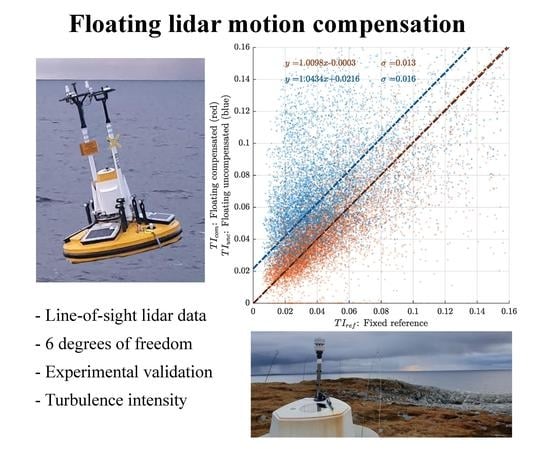
Taking the Motion out of Floating Lidar: Turbulence Intensity Estimates with a Continuous-Wave Wind Lidar


Abstract
:
1. Introduction
2. Theory
2.1. Turbulence Intensity
2.2. Coordinate System and Vector Rotations
2.3. The Motion-Induced Error in TI Measurements
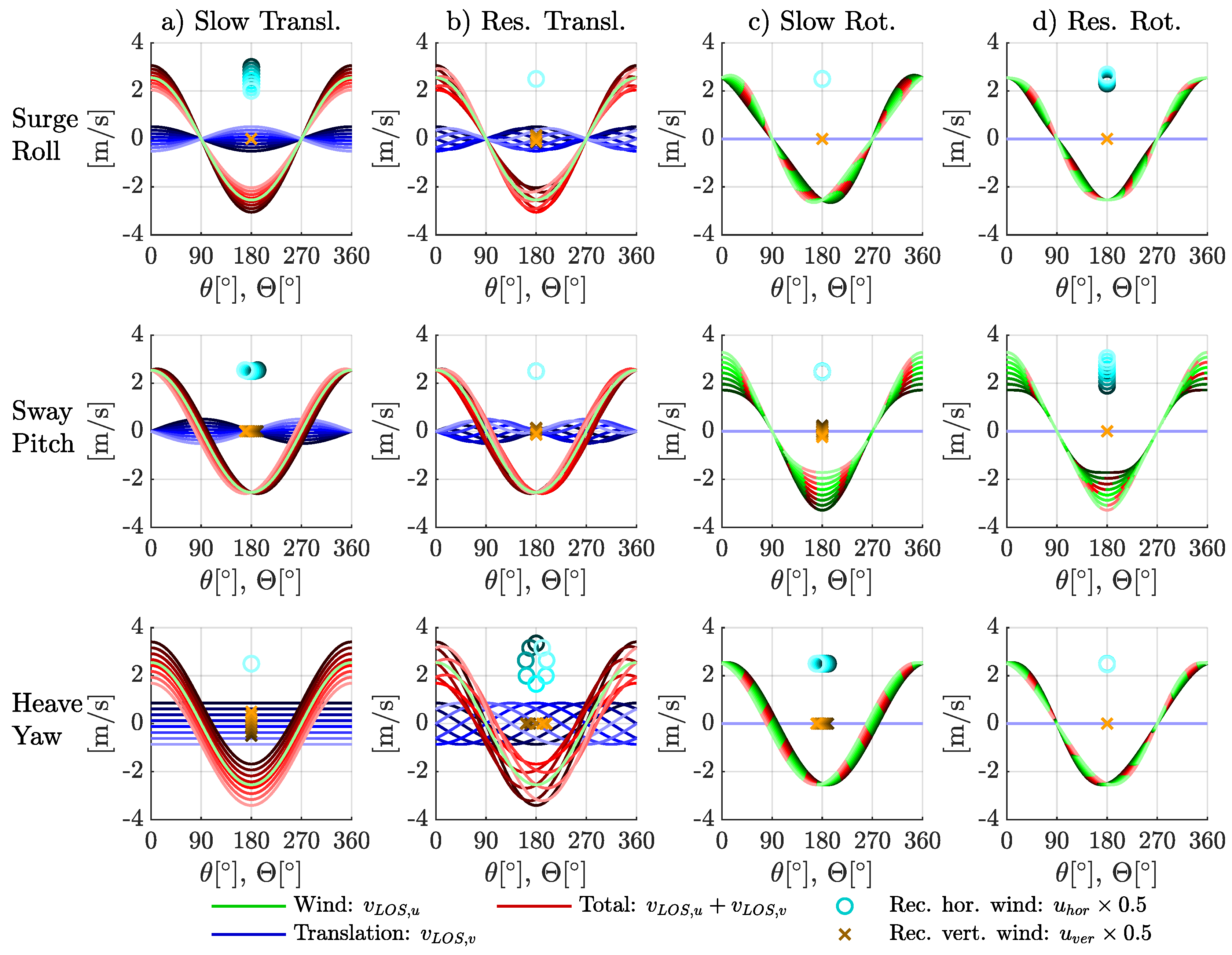
2.3.1. Error in Radial Velocities due to Translational Motion
2.3.2. Change in Scanning Geometry due to Rotational Motion
2.3.3. Changing Measurement Elevation due to Rotation under the Influence of Wind Shear and Veer
3. Method
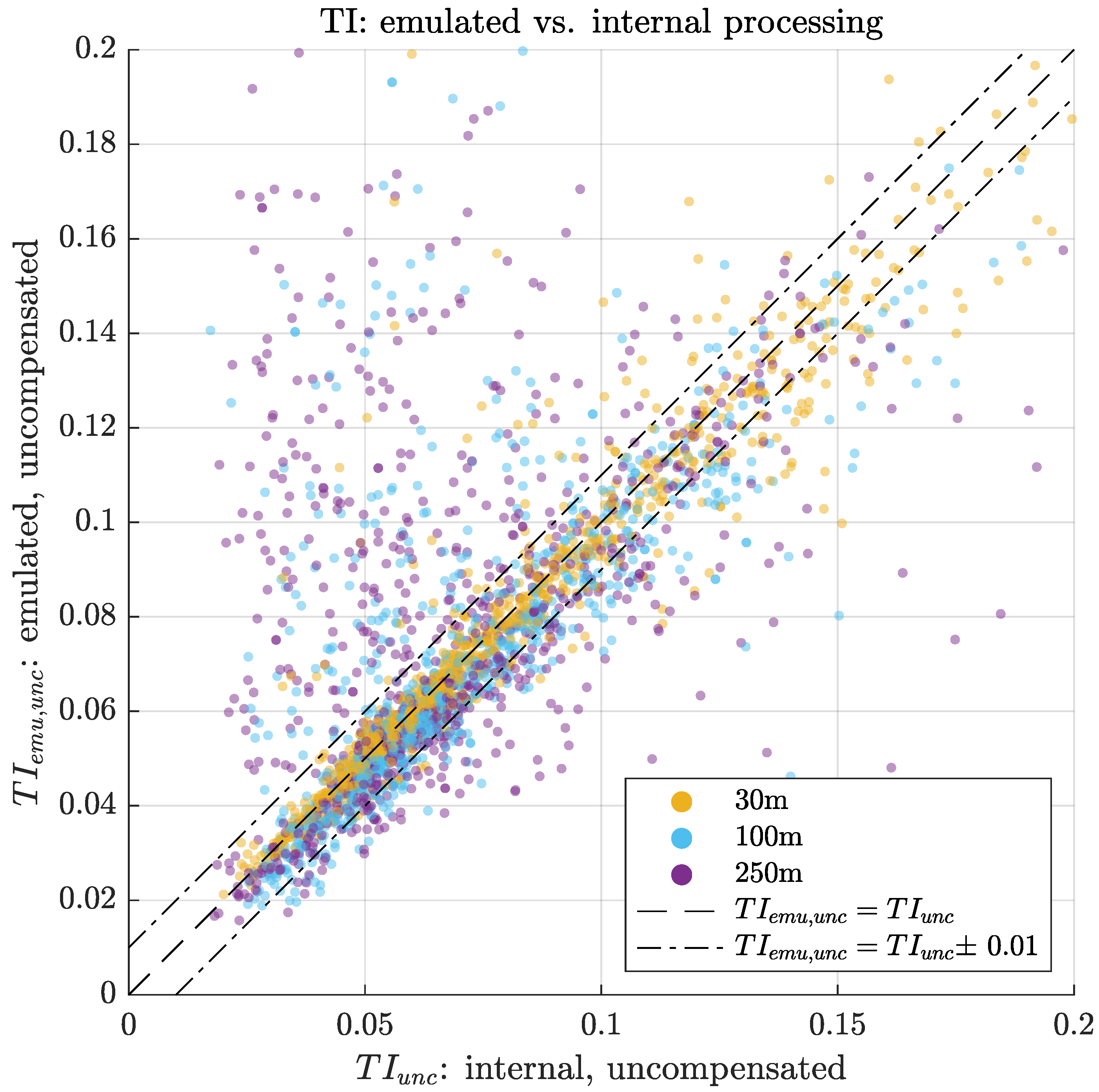
3.1. Emulation of Conventional VAD Processing
3.2. The Motion Compensation Algorithm
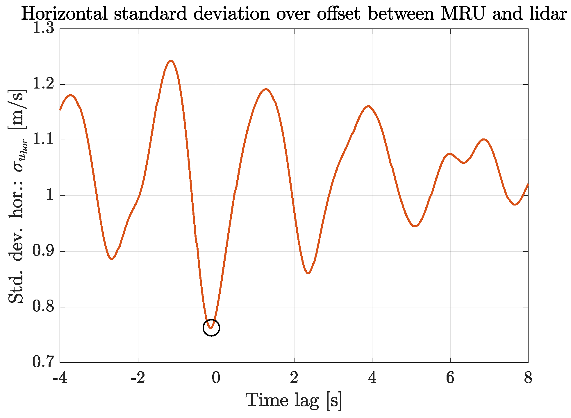
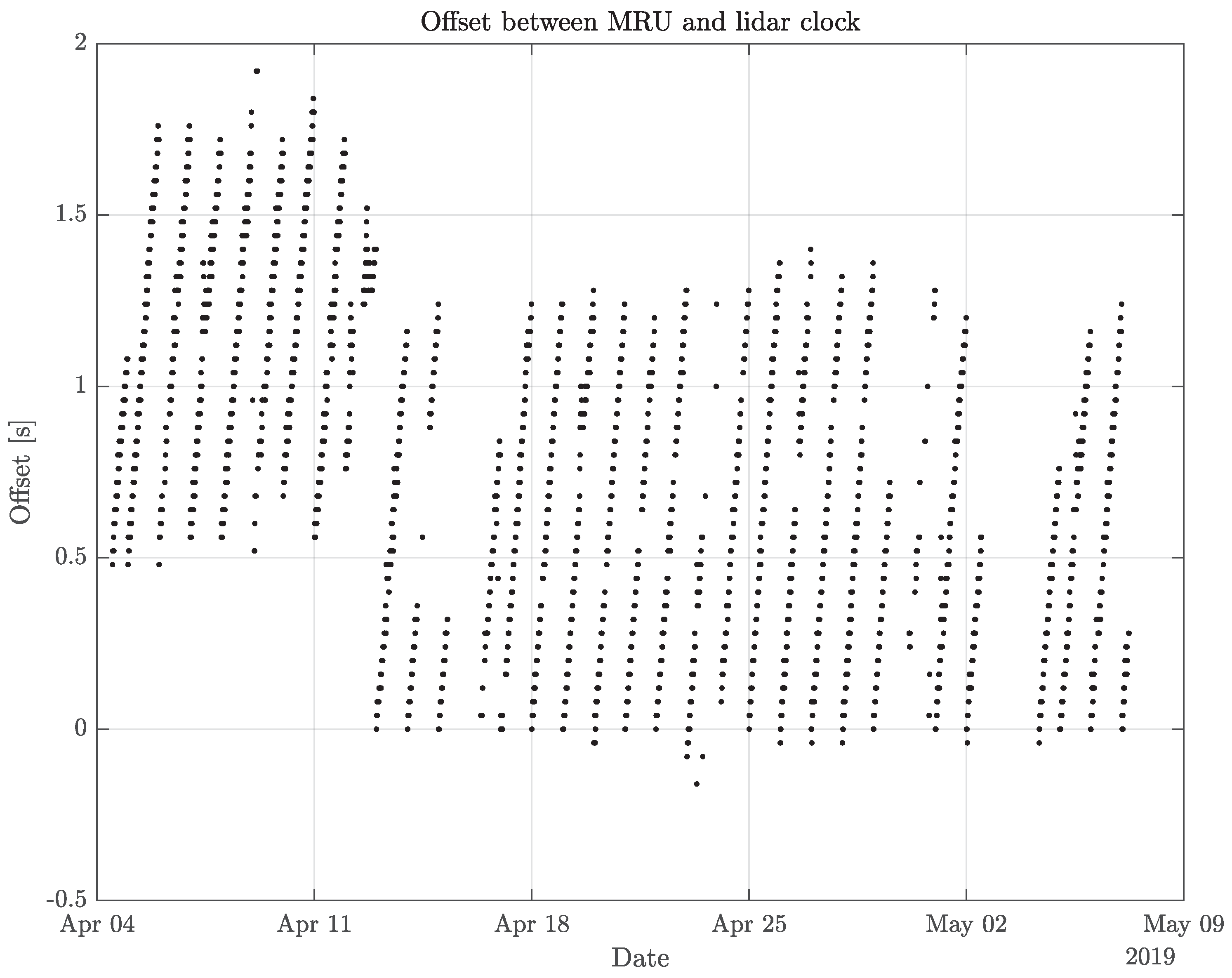
3.3. Time Synchronization
3.4. Data Handling
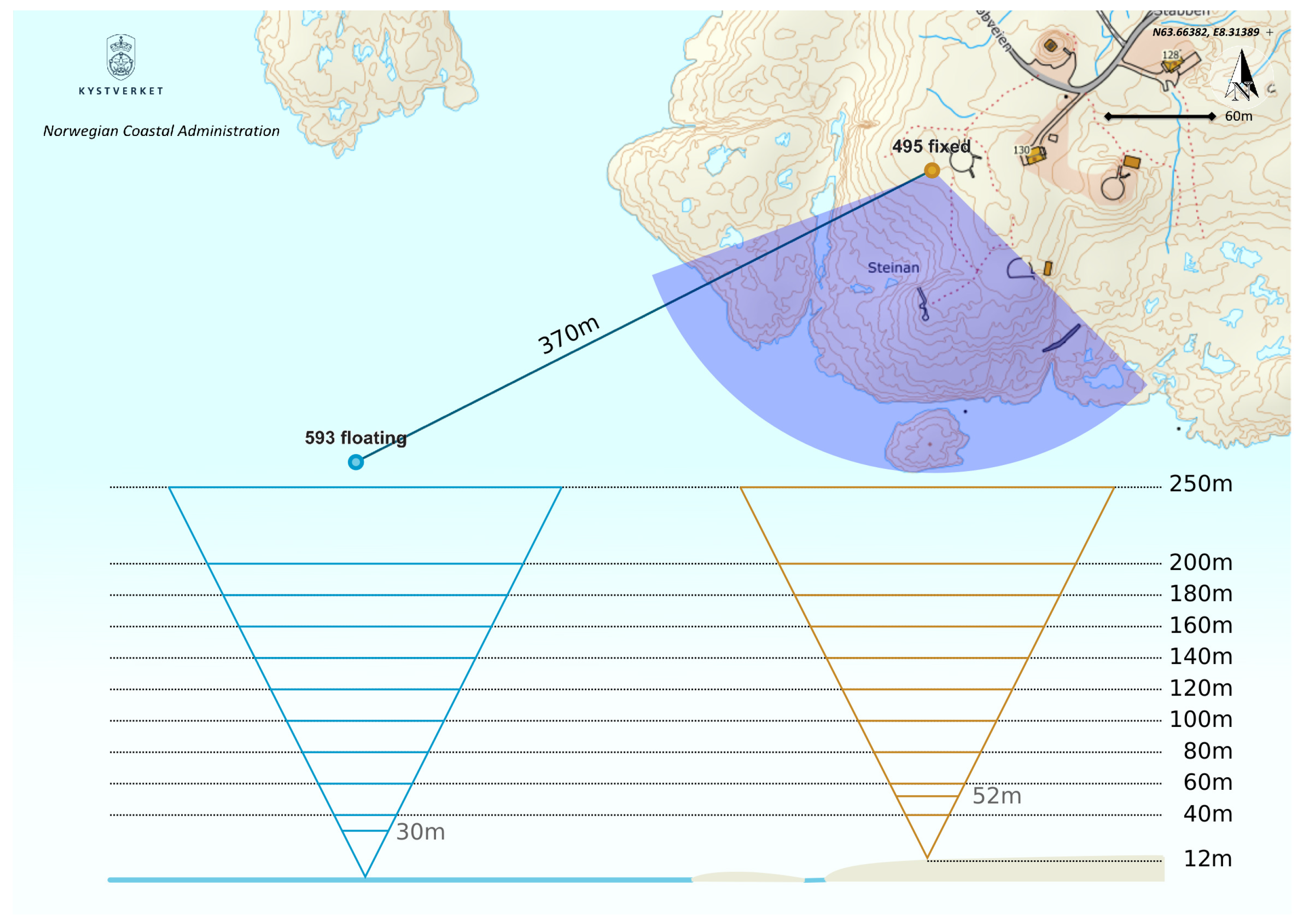
3.5. Instrumentation and Measurement Setup
3.6. Data Filtering
3.7. Measurement Uncertainty
4. Results and Discussion
4.1. Mean Wind
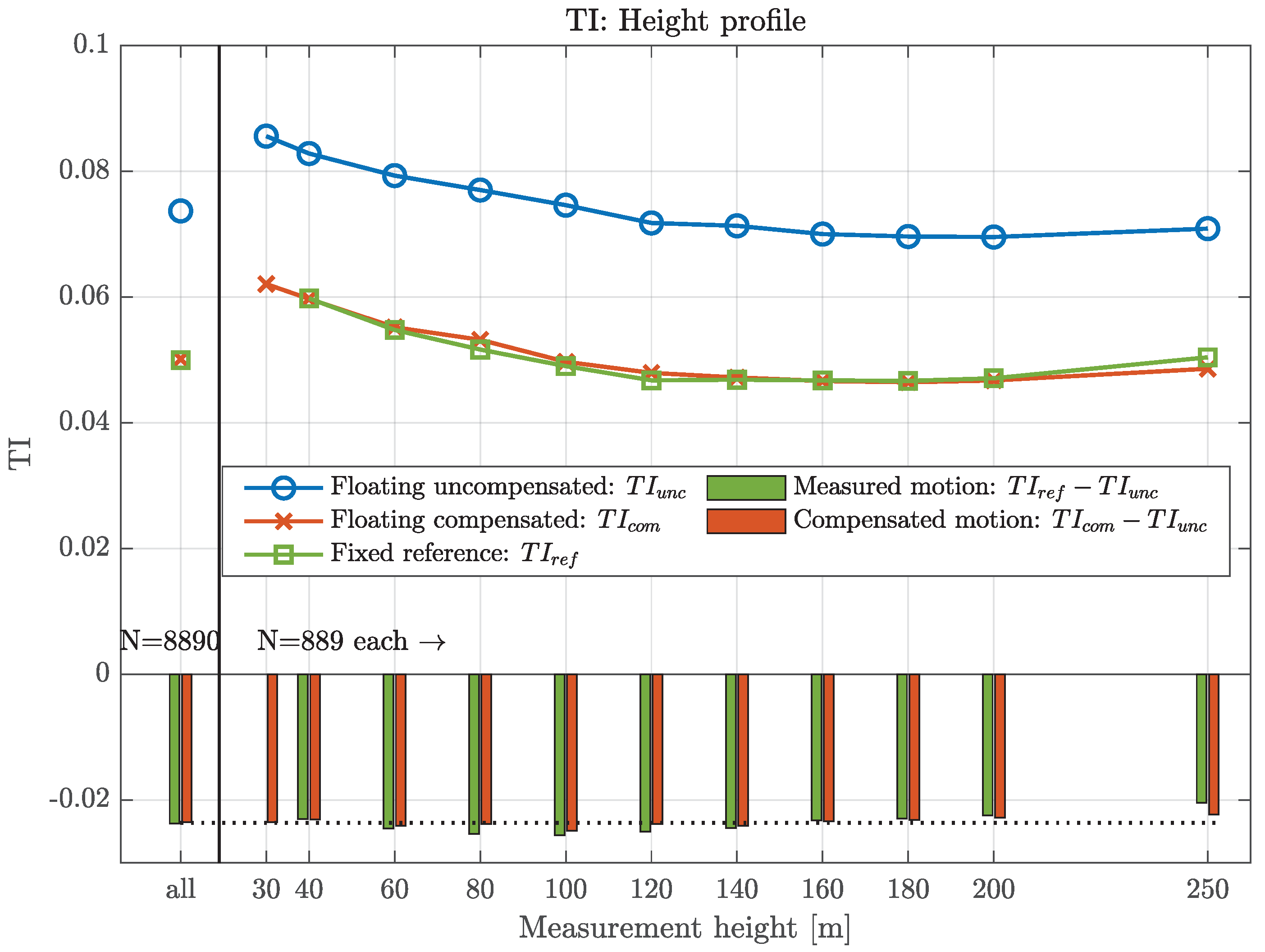
4.2. TI Profile
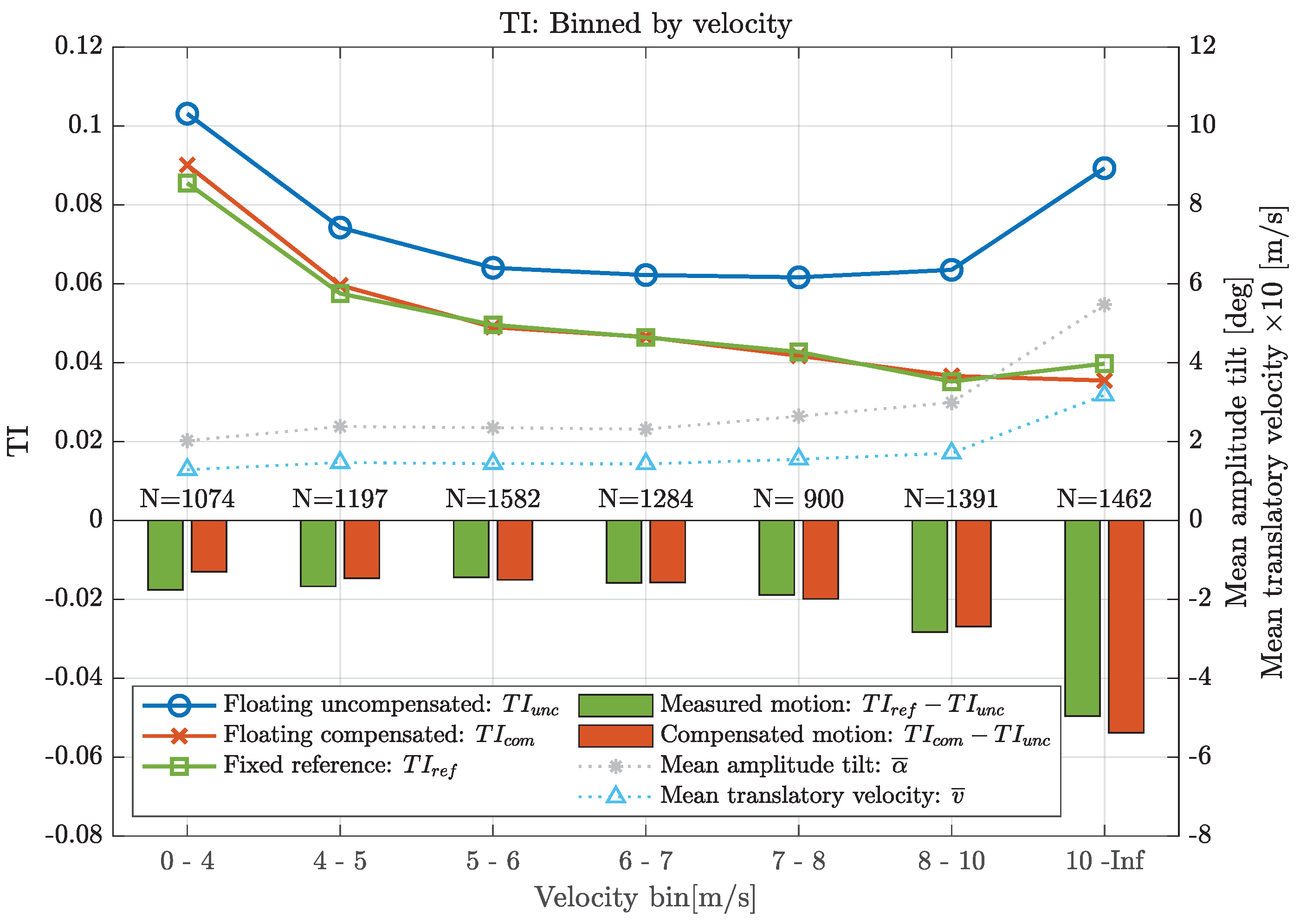
4.3. TI vs. Velocity
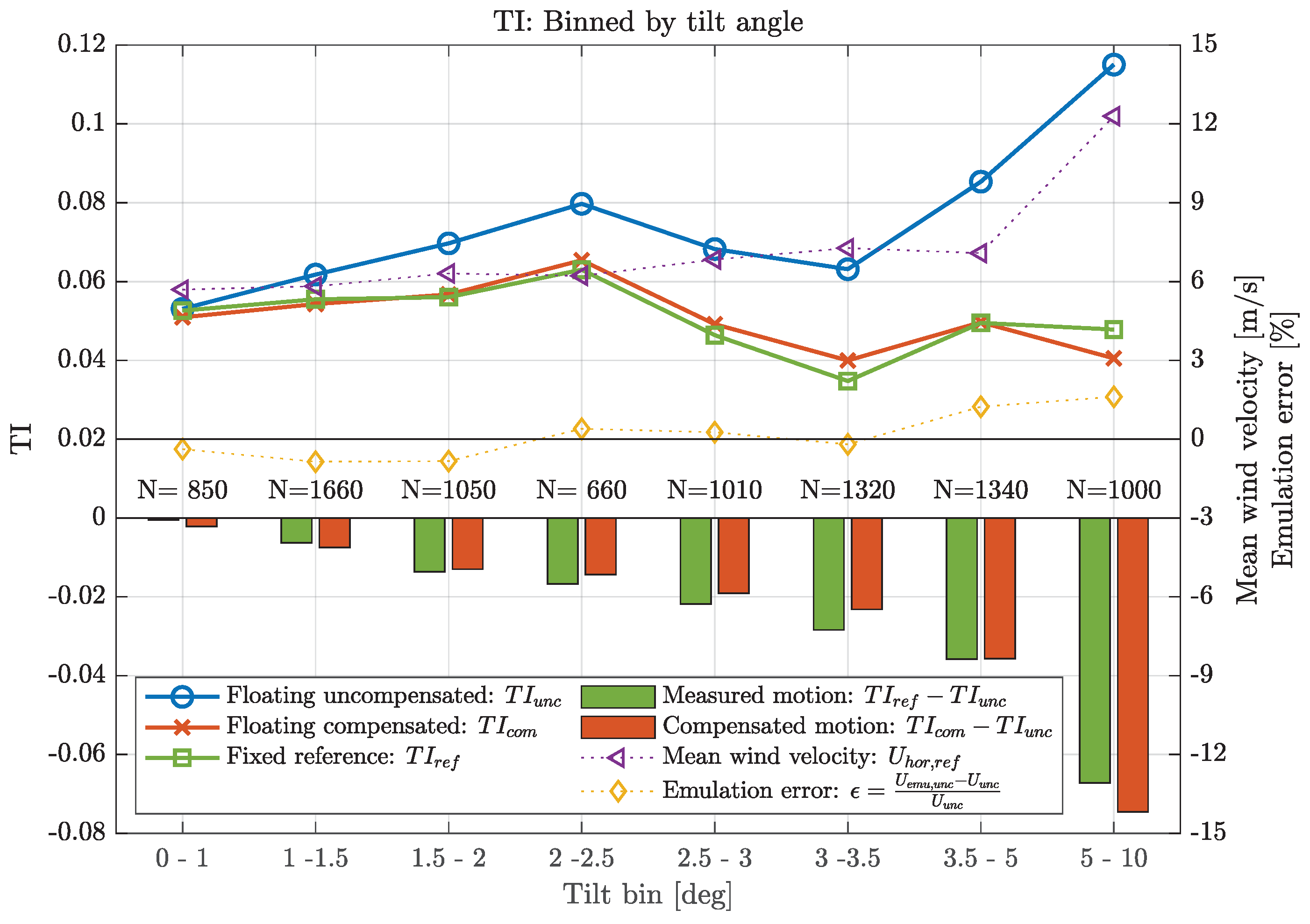
4.4. TI vs. Tilt Angle
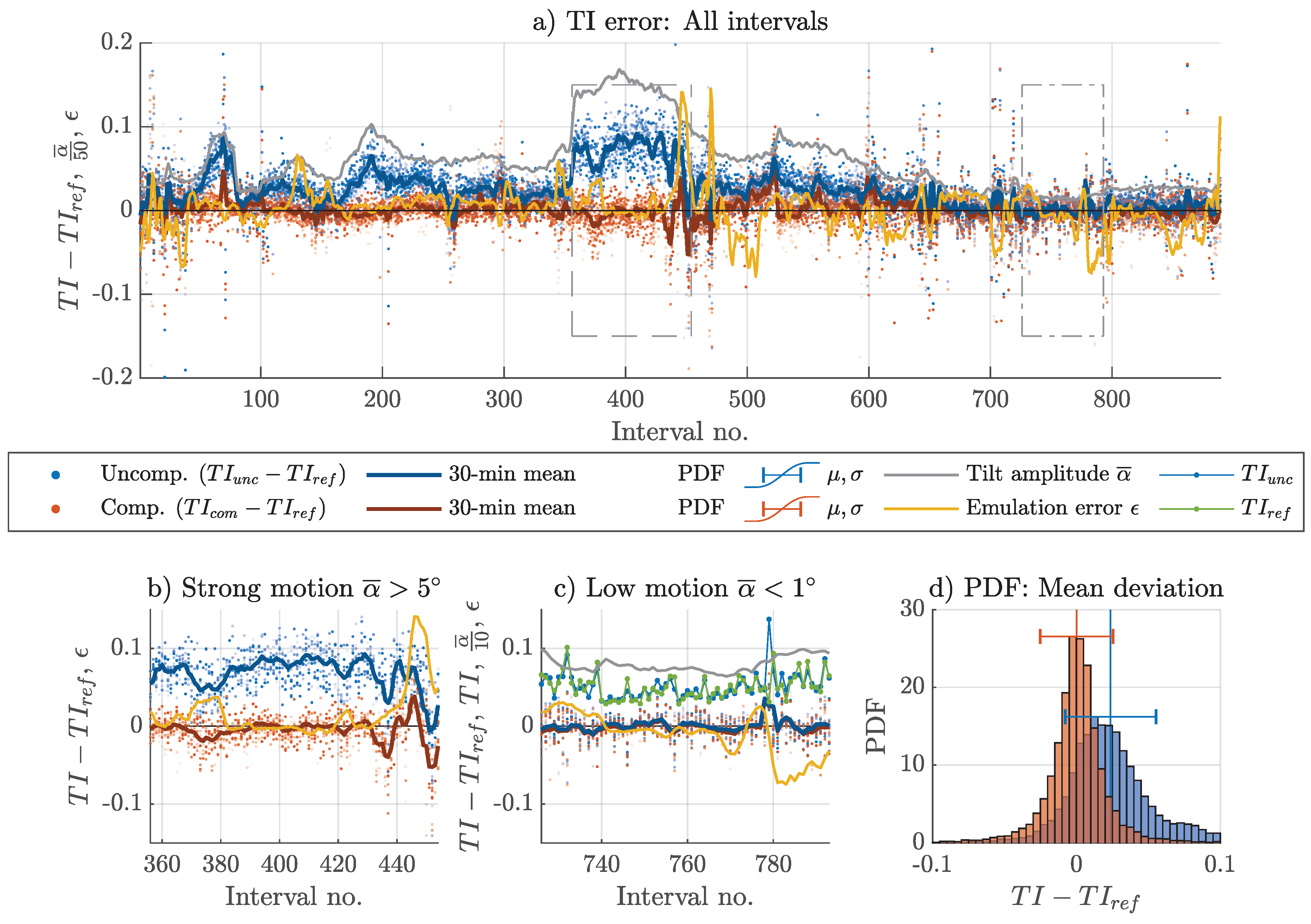
4.5. Individual Error Analysis
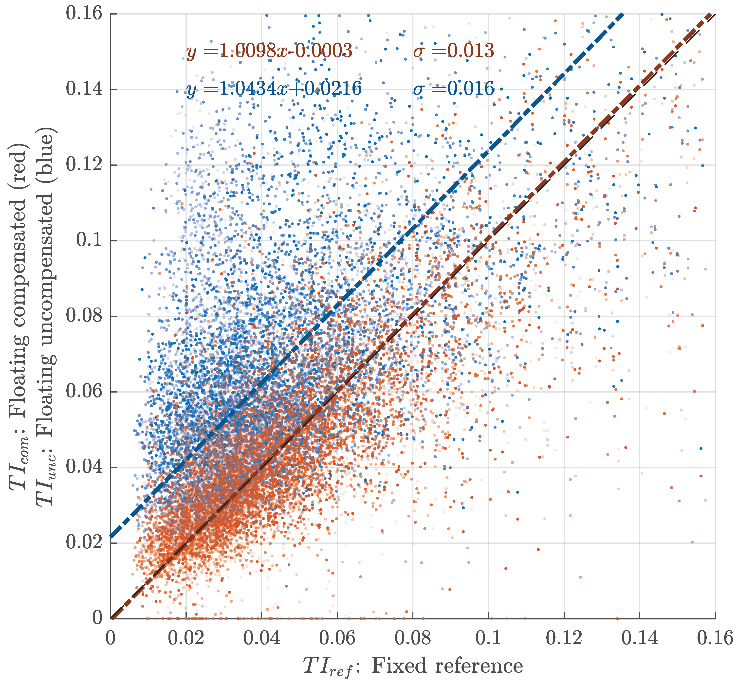
4.6. Scatter Analysis
5. Conclusions
Author Contributions
Funding
Acknowledgments
Conflicts of Interest
Abbreviations
| LOS | Line-of-sight |
| MRU | Motion reference unit |
| NWU | North-west-up |
| Res. | Resonance |
| Rot. | Rotational |
| Std. dev. | Standard deviation |
| Turbulence intensity | |
| Transl. | Translational |
| VAD | Velocity–azimuth display |
References
- Petersen, S.; Sarmento, A.; Cândido, J.; Godreau, C. Preliminary study on an offshore wind energy resource monitoring system. In Renewable Energies Offshore; Soarez, C.G., Ed.; Taylor & Francis: Abingdon, UK, 2015; pp. 213–218. [Google Scholar]
- Gottschall, J.; Gribben, B.; Stein, D.; Würth, I. Floating lidar as an advanced offshore wind speed measurement technique: Current technology status and gap analysis in regard to full maturity. WIREs Energy Environ. 2017, 6. [Google Scholar] [CrossRef]
- The Carbon Trust. Carbon Trust Offshore Wind Accelerator Roadmap for the Commercial Acceptance of Floating LiDAR Technology. Version 2.0. October 2018. [Google Scholar]
- Tiana-Alsina, J.; Rocadenbosch, F.; Gutiérrez-Antuñano, M.A. Vertical azimuth display simulator for wind-Doppler lidar error assessment. In Proceedings of the 2017 IEEE International Geoscience and Remote Sensing Symposium (IGARSS), Fort Worth, TX, USA, 23–28 July 2017; pp. 1614–1617. [Google Scholar] [CrossRef] [Green Version]
- Gottschall, J.; Wolken-Möhlmann, G.; Viergutz, T.; Lange, B. Results and conclusions of a floating-lidar offshore test. Energy Procedia 2014, 53, 156–161. [Google Scholar] [CrossRef]
- Mathisen, J.P. Measurement of wind profile with a buoy mounted lidar. In Proceedings of the 10th Deep Sea Offshore Wind R&D Conference, DeepWind’2013, Trondheim, Norway, 24–25 January 2013. [Google Scholar]
- Gutiérrez-Antuñano, M.A.; Tiana-Alsina, J.; Salcedo, A.; Rocadenbosch, F. Estimation of the Motion-Induced-Horizontal-Wind-Speed Standard Deviation in an Offshore Doppler Lidar. Remote Sens. 2018, 10, 2037. [Google Scholar] [CrossRef] [Green Version]
- Tiana-Alsina, A.J.; Gutiérrez, M.A.; Würth, I.; Puigdefábregas, J.; Rocadenbosch, F. Motion compensation study for a floating Doppler wind LiDAR. In Proceedings of the 2015 IEEE International Geoscience and Remote Sensing Symposium (IGARSS), Milan, Italy, 26–31 July 2015. [Google Scholar] [CrossRef]
- Gutiérrez, M.A.; Tiana-Alsina, J.; Bischoff, O.; Cateura, J.; Rocadenbosch, F. Performance evaluation of a floating Doppler wind lidar buoy in mediterranean near-shore conditions. In Proceedings of the 2015 IEEE International Geoscience and Remote Sensing Symposium (IGARSS), Milan, Italy, 26–31 July 2015. [Google Scholar] [CrossRef]
- Yamaguchi, A.; Ishihara, T. A new motion compensation algorithm of floating lidar system for the assessment of turbulence intensity. J. Phys. Conf. Ser. 2016, 753. [Google Scholar] [CrossRef]
- Gottschall, J.; Wolken-Möhlmann, G.; Lange, B. About offshore resource assessment with floating lidars with special respect to turbulence and extreme events. J. Phys. Conf. Ser. 2014, 555. [Google Scholar] [CrossRef]
- Sathe, A.; Mann, J.; Gottschall, J.; Courtney, M.S. Can wind lidars measure turbulence? J. Atmos. Ocean. Tech. 2011, 853–868. [Google Scholar] [CrossRef] [Green Version]
- Kelberlau, F.; Mann, J. Better turbulence spectra from velocity-azimuth display scanning wind lidar. Atmos. Meas. Tech. 2019, 12, 1871–1888. [Google Scholar] [CrossRef] [Green Version]
- Kelberlau, F.; Mann, J. Cross-contamination effect on turbulence spectra from Doppler beam swinging wind lidar. Wind Energy Sci. Discuss. 2019. [Google Scholar] [CrossRef] [Green Version]
- Emeis, S. Wind Energy Meteorology, 2nd ed.; Springer International Publishing AG: Berlin/Heidelberg, Germany, 2018. [Google Scholar] [CrossRef]
- Grewal, M.S.; Weill, P.L.R.; Andrews, A.P. Global Positioning Systems, Inertial Navigation, and Integration; chapter Appendix C: Coordinate Transformations; John Wiley & Sons Inc.: Hoboken, NJ, USA, 2006; pp. 456–501. [Google Scholar] [CrossRef] [Green Version]
- Cole, I.R. Modelling CPV. Ph.D. Thesis, Loughborough University, Loughborough, UK, 2015. [Google Scholar]
- Gottschall, J.; Catalano, E.; Dörenkämper, M.; Witha, B. The NEWA Ferry Lidar Experiment: Measuring Mesoscale Winds in the Southern Baltic Sea. Remote Sens. 2018, 10, 1620. [Google Scholar] [CrossRef] [Green Version]
- Zhai, X.; Wu, S.; Liu, B.; Song, X.; Yin, J. Shipborne Wind Measurement and Motion-induced Error Correction of a Coherent Doppler Lidar over the Yellow Sea in 2014. Atmos. Meas. Tech. 2018, 11, 1313–1331. [Google Scholar] [CrossRef] [Green Version]
- Wolken-Möhlmann, G.; Lilov, H.; Lange, B. Simulation of Motion Induced Measurement Errors for Wind Measurements Using LIDAR on Floating Platforms; Fraunhofer IWES: Bremerhaven, Germany, 2010. [Google Scholar]
- Branlard, E.; Pedersen, A.T.; Mann, J.; Angelou, N.; Fischer, A.; Mikkelsen, T.; Harris, M.; Slinger, C.; Montes, B. Retrieving wind statistics from average spectrum of continuous-wave lidar. Atmos. Meas. Tech. 2013, 6, 1673–1683. [Google Scholar] [CrossRef] [Green Version]
- Angelou, N.; Foroughi Abari, F.; Mann, J.; Mikkelsen, T.; Sjöholm, M. Challenges in noise removal from Doppler spectra acquired by a continuous-wave lidar. In Proceedings of the 26th International Laser Radar Conference, Porto Heli, Greece, 25–29 June 2012. [Google Scholar]
- Pitter, M.; Slinger, C.; Harris, M. Introduction to continuous-wave Doppler lidar. In Remote Sensing for Wind Energy; DTU Wind Energy-E-Report-E-0084; DNV GL-Energy: Kaiser-Wilhelm-Koog, Germany, 2015. [Google Scholar]
- Mann, J.; Peña, A.; Bingöl, F.; Wagner, R.; Courtney, M.S. Lidar scanning of momentum flux in and above the surface layer. J. Atmos. Ocean. Technol. 2010, 27, 959–976. [Google Scholar] [CrossRef]
- Dellwik, E.; Mann, J.; Bingöl, F. Flow tilt angles near forest edges – Part 2: Lidar anemometry. Biogeosciences 2010, 7, 1759–1768. [Google Scholar] [CrossRef] [Green Version]
- Mark, A.; Köhne, V.; Stein, D. Assessment of the Fugro OCEANOR Seawatch Wind LiDAR Buoy WS 170 Pre-Deployment Validation at Frøya, Norway; Technical Report GLGH-4270 17 14462-R-0002, Rev. C; DNV GL-Energy: Kaiser-Wilhelm-Koog, Germany, 2017. [Google Scholar]
- Wylie, S. Turbulence Intensity measurements from a ground-based vertically-profiling lidar. In Proceedings of the WindEurope Resource Assessment Workshop Session 4: Using Lidar to Reduce Uncertainty, Brussels, Belgium, 27–28 June 2019. [Google Scholar]
- Türk, M.; Emeis, S. The dependence of offshore turbulence intensity on wind speed. J. Wind Eng. Ind. Aerodyn. 2010, 98, 466–471. [Google Scholar] [CrossRef]
- Svensson, N.; Arnqvist, J.; Bergström, H.; Rutgersson, A.; Sahlée, E. Measurements and Modelling of Offshore Wind Profiles in a Semi-Enclosed Sea. Atmosphere 2019, 10, 194. [Google Scholar] [CrossRef] [Green Version]
- Adcock, R.J. A Problem in Least Squares. Analyst 1878, 5, 53–54. [Google Scholar] [CrossRef]
- Cornbleet, P.J.; Gochman, N. Incorrect least-squares regression coefficients in method-comparison analysis. Clin. Chem. 1979, 25, 432–438. [Google Scholar] [CrossRef] [PubMed]
- Abari, C.F.; Pedersen, A.T.; Mann, J. An all-fiber image-reject homodyne coherent Doppler wind lidar. Opt. Express 2014, 22, 25880–25894. [Google Scholar] [CrossRef] [PubMed] [Green Version]
- Gao, S.; Hui, R. Frequency-modulated continuous-wave lidar using I\Q modulator for simplified heterodyne detection. Opt. Lett. 2012, 37, 2022–2024. [Google Scholar] [CrossRef] [PubMed] [Green Version]


| Name | Symbol | Mean | Min | Max | Std. dev. | Unit |
|---|---|---|---|---|---|---|
| Mean wind speed | U | 7.2 | 1.4 | 22.1 | 3.2 | [] |
| Turbulence intensity | 5.0 | 0.6 | 41.6 | 3.7 | [%] | |
| Mean dynamic tilt angle | 2.91 | 0.62 | 8.73 | 1.84 | ] | |
| Mean tilt period | 2.51 | 2.11 | 2.70 | 0.10 | [] | |
| Mean heave velocity | 0.13 | 0.03 | 0.41 | 0.08 | [] | |
| Mean heave displacement | 0.12 | 0.03 | 0.41 | 0.08 | [] |
© 2020 by the authors. Licensee MDPI, Basel, Switzerland. This article is an open access article distributed under the terms and conditions of the Creative Commons Attribution (CC BY) license (http://creativecommons.org/licenses/by/4.0/).
Share and Cite
Kelberlau, F.; Neshaug, V.; Lønseth, L.; Bracchi, T.; Mann, J. Taking the Motion out of Floating Lidar: Turbulence Intensity Estimates with a Continuous-Wave Wind Lidar. Remote Sens. 2020, 12, 898. https://0-doi-org.brum.beds.ac.uk/10.3390/rs12050898
Kelberlau F, Neshaug V, Lønseth L, Bracchi T, Mann J. Taking the Motion out of Floating Lidar: Turbulence Intensity Estimates with a Continuous-Wave Wind Lidar. Remote Sensing. 2020; 12(5):898. https://0-doi-org.brum.beds.ac.uk/10.3390/rs12050898
Chicago/Turabian StyleKelberlau, Felix, Vegar Neshaug, Lasse Lønseth, Tania Bracchi, and Jakob Mann. 2020. "Taking the Motion out of Floating Lidar: Turbulence Intensity Estimates with a Continuous-Wave Wind Lidar" Remote Sensing 12, no. 5: 898. https://0-doi-org.brum.beds.ac.uk/10.3390/rs12050898