Evaluation and Comparison of Light Use Efficiency and Gross Primary Productivity Using Three Different Approaches


1
State Key Laboratory of Remote Sensing Science, Faculty of Geographical Science, Beijing Normal University, Beijing 100875, China
2
Beijing Engineering Research Center for Global Land Remote Sensing Products, Faculty of Geographical Science, Beijing Normal University, Beijing 100875, China
*
Author to whom correspondence should be addressed.
Remote Sens. 2020, 12(6), 1003; https://0-doi-org.brum.beds.ac.uk/10.3390/rs12061003
Submission received: 3 February 2020
/
Revised: 7 March 2020
/
Accepted: 17 March 2020
/
Published: 20 March 2020
(This article belongs to the Special Issue Advances of Multi-Temporal Remote Sensing in Vegetation and Agriculture Research)
Abstract
:Light use efficiency (LUE), which characterizes the efficiency with which vegetation converts captured/absorbed radiation into organic dry matter through photosynthesis, is a key parameter for estimating vegetation gross primary productivity (GPP). Studies suggest that diffuse radiation induces a higher LUE than direct radiation in short-term and site-scale experiments. The clearness index (CI), described as the fraction of solar incident radiation on the surface of the earth to the extraterrestrial radiation at the top of the atmosphere, is added to the parameterization approach to explain the conditions of diffuse and direct radiation in this study. Machine learning methods—such as the Cubist regression tree approach—are also popular approaches for studying vegetation carbon uptake. This paper aims to compare and analyze the performances of three different approaches for estimating global LUE and GPP. The methods for collecting LUE were based on the following: (1) parameterization approach without CI; (2) parameterization approach with CI; and (3) Cubist regression tree approach. We collected GPP and meteorological data from 180 FLUXNET sites as calibration and validation data and the Global Land Surface Satellite (GLASS) products and ERA-interim data as input data to estimate the global LUE and GPP in 2014. Site-scale validation with FLUXNET measurements indicated that the Cubist regression approach performed better than the parameterization approaches. However, when applying the approaches to global LUE and GPP, the parameterization approach with the CI became the most reliable approach, then closely followed by the parameterization approach without the CI. Spatial analysis showed that the addition of the CI improved the LUE and GPP, especially in high-value zones. The results of the Cubist regression tree approach illustrate more fluctuations than the parameterization approaches. Although the distributions of LUE presented variations over different seasons, vegetation had the highest LUE, at approximately 1.5 gC/MJ, during the whole year in equatorial regions (e.g., South America, middle Africa and Southeast Asia). The three approaches produced roughly consistent global annual GPPs ranging from 109.23 to 120.65 Pg/yr. Our results suggest the parameterization approaches are robust when extrapolating to the global scale, of which the parameterization approach with CI performs slightly better than that without CI. By contrast, the Cubist regression tree produced LUE and GPP with lower accuracy even though it performed the best for model validation at the site scale.
1. Introduction
Estimations of global vegetation productivity are essential for improving the understanding of the interaction between the terrestrial biosphere and the atmosphere in the context of global changes and the further formulation of climate policy decisions [1,2]. GPP, a key variable in the global carbon cycle, is influenced by various factors such as temperature [3], soil moisture [4], vegetation types and even tree species [5], crop types [6], tree ages [7] and radiation [8]. To date, many models, including process models and LUE-based models, have been established to estimate global GPP; however, they vary greatly in terms of produced values [9,10,11,12,13,14,15,16,17,18].
Currently, some GPP models try to build the relationships between GPP and climate factors, FPAR and the vegetation indices with which global GPP is produced [19,20,21]. However, those models don’t care about the intermediate variable LUE and its impact on GPP. LUE is of great significance in GPP estimation, and it can help us to deeply understand and clarify the key processes of the vegetation carbon sequestration. This paper focuses on the estimation of LUE based on remote sensing data, and then explores its impact on GPP estimation. The LUE-based model was originally described by Monteith [22,23]. It has a simple formula and can present consistent ecosystem processes across various vegetation types [24,25], which makes it the most promising method for adequately addressing the spatial and temporal dynamics of GPP. The input data, such as the fraction of absorbed photosynthetically active radiation (FPAR), could be produced by remote sensing techniques. Therefore, it has been widely used to estimate GPP at local, regional and global scales [3,26,27,28,29].
LUE is defined as the ratio of carbon uptake to absorbed photosynthetically active radiation (APAR) for a plant canopy [30]. The dominant methods used to determine LUE are based on environmental stress factors and vegetation spectral indexes. The photochemical reflectance index (PRI), as one popular vegetation spectral index, is a good estimator of LUE, especially in the short-term [31,32] and at the leaf/canopy scale [33,34]. However, confounding factors appear at larger temporal and spatial scales. The correlations of PRI with LUE varied dramatically throughout the growing season [35] and were decoupled in severe circumstances, consequently leading to an overestimation of LUE [36]. Some studies process temperature and water stress factors based on the parameterization approach [37] and machine learning methods [38], and have obtained high-quality LUE values.
The LUE-based GPP model is built upon two fundamental assumptions: (1) GPP equals the product of APAR and LUE; (2) actual LUE may be reduced below its potential value by environmental stresses such as low temperatures or water shortages. Consequently, the accuracy of the LUE greatly influences the quality of the GPP. However, it is quite difficult to accurately calculate global LUE because it cannot be directly measured and is sensitive to various factors. In different models, parameters such as temperatures or water stress factors are described in different ways, which leads to significant variations in the estimation results. The evaporative fraction (EF) is widely used as a water stress factor in LUE and GPP models [39]. Zhang et al. (2015) [40] showed that LUE was more responsive to plant moisture indicators, such as plant EF, than to atmospheric indicators, such as the vapor pressure deficit (VPD).
Previous studies suggest that the efficiency of carbon uptake is usually higher under diffuse light (cloudy or hazy skies) than under direct light (clear sky) [41,42]. The underlying mechanism for this growth is the increased penetration of light into deeper layers of the canopy under diffuse light [8]. In contrast, clouds may reduce the total radiation, which would lead to the reduction of PAR and GPP [43]. Therefore, the effect of radiation mode on LUE and GPP is complicated. Furthermore, previous studies have mostly focused on short-term [44] and site-scale [43,45] LUE and GPP. The CI, described as the fraction of solar incident radiation on the surface of the earth to the extraterrestrial radiation at the top of the atmosphere [35,46], is an effective way to explain the circumstances of diffuse and direct light. This index prompts our motivation to explore the influences of the CI on long-term and global LUE and GPP.
Machine learning methods provide a powerful tool to upscale site-observed fluxes to a larger scale with satellite-derived parameters and other explanatory variables [37]. The application of the Cubist regression tree approach in vegetation carbon uptake research is a good example. The main advantage of the Cubist method is to add multiple training committees and “reinforcement”, so as to make the weights more balanced [47]. It also provides linear equations for prediction instead of black box. In addition, Cubist is a commercial, proprietary product and has the least algorithmic documentation [48]. Houborg et al. prove the better performances than random forest in estimating leaf area index [49]. Previous studies use this approach to produce LUE, GPP and spatially continuous GPP in the USA [50,51,52,53], and these studies gain satisfactory validation results against site-scale measured GPP. However, few studies compare this approach with the parameterization approach in terms of global LUE and GPP.
The purpose of this paper is to compare and analyze the performances of different approaches for producing global and seasonal LUE and GPP. The three methods for determining LUE were based on (1) a parameterization approach without the CI, (2) a parameterization approach with the CI, and 3) the Cubist regression tree approach. We collected eddy-covariance and meteorological data from 180 FLUXNET sites as calibration and validation data and GLASS products and ERA-interim data as input data to estimate global LUE and GPP in 2014, with a spatial resolution of 5 km and a temporal resolution of 8 days. FLUXNET measurements were used to validate LUE and GPP using three approaches at the site scale. Furthermore, we compared the temporal and spatial patterns of the LUE and GPP to analyze and assess the strengths and drawbacks of each approach. It is worth noting that global LUE distributions were first presented in this study to explore the spatial variations in LUE in different areas and the temporal changes in LUE in different seasons.
2. Materials and Methods
2.1. Data Collection
2.1.1. Data from FLUXNET
The FLUXNET2015 dataset, which can be downloaded from https://fluxnet.fluxdata.org/data/, contains global eddy covariance measurements and meteorological variables from more than 200 sites. In this study, we selected daily GPP, incident shortwave radiation (SW), latent heat flux (LE), sensible heat flux (H) and hourly air temperature (TA). FLUXNET GPP is calculated as the difference between ecosystem respiration (RECO) and net ecosystem CO2 exchange (NEE). SW was used to calculate PAR by multiplying the value by 0.48 [54]. LE and H were prepared for the EF according to EF = LE/(LE+H). Mean temperature (Tmean) was obtained by averaging hourly TA. To ensure that the FLUXNET data were reliable, we retained only high-quality data with the help of quality flags. Finally, we obtained 29,056 pieces of data distributed at 180 sites ranging from 2003 to 2014. All data were distributed in 12 types of vegetation, of which CRO (croplands) had 20 sites, CSH (closed shrublands) had 3 sites, DBF (deciduous broadleaf forests) had 24 sites, DNF (deciduous needleleaf forests) had 1 site, EBF (evergreen broadleaf forests) had 10 sites, ENF (evergreen needleleaf forests) had 35 sites, GRA (grasslands) had 33 sites, MF (mixed forests) had 9 sites, OSH (open shrublands) had 14 sites, SAV (savannas) had 7 sites, WET (permanent wetlands) had 18 sites, and WSA (woody savannas) had 6 sites. In this study, we considered WET as GRA because of the complicated conditions of WET.
2.1.2. MODIS Data Processing
We downloaded the fraction of absorbed photosynthetically active radiation (FPAR) and leaf area index (LAI) (MCD15A2H) data of Moderate Resolution Imaging Spectroradiometer (MODIS) at a spatial resolution of 500 m (from MODIS Global Subsets website https://modis.ornl.gov/cgi-bin/MODIS/global/subset.pl), with which LUE was calculated according to Formula (1) in the FLUXNET sites:
where GPP and SW were from the FLUXNET data, and FPAR was from the MODIS data at a resolution of 500 m. 0.48 represents the ratio of photosynthetically active radiation to the total incoming solar energy. At each site, 9 (3 × 3) pixels around the central position were collected for quality-control processes. The first quality-control process included (1) gaining 9 values in each site; (2) deleting invalid data according to the quality control flags; (3) counting the number of valid values in each site; and (4) retaining the valid data if the number exceeds 5, or deleting the valid data if the value did not.
MODIS LAI and FPAR depend on the reflectance in the red, near-infrared (NIR), and sometimes shortwave infrared (SWIR) bands at the surface level, which are often very sensitive to atmospheric effects, including clouds, aerosols, water vapor, and ozone [55,56]. Although many of these effects can be removed using real-time or near real-time atmospheric observations [57], the remaining effects can sometimes be very large. These remaining effects generally cause more increases in the red band than in the NIR band, consequently resulting in the reduction of LAI and FPAR. In this case, there would be abnormally low values in a seasonal trajectory. Therefore, we conduct the second quality-control process, which includes deleting abnormally low values based on seasonal curves [58]. In parameterization approaches, parameters, for example, maximum LUE, vary with vegetation type.
In the regression tree approach, vegetation type can be an input data used to calibrate the approach. We used the International Geosphere-Biosphere Programme (IGBP) vegetation type map from yearly global 5-km MODIS Landcover (MCD12C1) to address different types of vegetation. In addition, we downloaded MOD17 8-day/0.05 degree GPP as an existing global GPP product to analyze our GPP from http://files.ntsg.umt.edu/data/NTSG_Products/MOD17 [59].
2.1.3. GLASS Data
The GLASS LAI and FPAR datasets were generated and released by Beijing Normal University (http://www.bnu-datacenter.com) [60]. This product has a temporal resolution of 8 days and is available from 1981 to the present. The LAI and FPAR used in this study were generated from AVHRR reflectance at a resolution of 5 km [61]. The GLASS LAI and FPAR products have smooth and reasonable trajectories. By cross-comparison and validation, the accuracy of GLASS products is clearly better than that of MODIS and CYCLOPES products (Carbon Cycle and Change in Land Observational Products from an Ensemble of Satellites). Moreover, the GLASS LAI and FPAR are more temporally continuous and spatially complete than are the other tested products [62,63].
2.1.4. ERA-Interim Data
ERA-Interim is a global land surface reanalysis dataset covering the period since 1979 and continuing in real time. This product can be downloaded from the European Centre for Medium Range Weather Forecasts (ECMWF) Data Server at http://data.ecmwf.int/data. The time steps are sub-daily, daily and monthly, and a spatial resolution of 0.75°. ERA-Interim is the result of the simulation with the latest ECMWF land surface model driven by meteorological forcing from the ERA-Interim atmospheric reanalysis and precipitation adjustments based on the monthly Global Precipitation Climatology Project (GPCP) [64]. In this study, we downloaded half-daily ERA average air temperature (AAT), 2-m dewpoint temperature (D2M), surface air pressure (P), downward shortwave radiation (SWdw), net longwave radiation (LWnet) and net shortwave radiation (SWnet). Then, we averaged every 16 values to obtain 8-day ERA data to prepare for the global LUE and GPP estimation.
2.2. Methods
LUE is of great significance in GPP estimation, and it can help us to deeply understand and clarify the key processes of the vegetation carbon sequestration. In this section, we will describe the different approaches of estimating LUE and then how to gain GPP based on LUE.
2.2.1. LUE Estimation
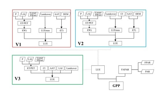
We established 3 approaches to compute LUE. Two of them were parameterization approaches in which we first determined the maximum LUE for each type of vegetation by an optimization algorithm developed at the University of Arizona (SCE-UA), and then we adjusted the maximum LUE with temperature and water stress factors, finally estimating the actual LUE. The difference between the two parameterization approaches was whether we considered the effect of solar radiation by adopting the CI in the determination of the maximum LUE. The third approach was the Cubist regression approach, which considers the contributions of temperature, LAI, EF, CI and vegetation type to the LUE.
• Parameterization approach without CI (approach V1)
LUE is estimated by Formula (2) in the parameterization approach without CI (approach V1):
where LUE is the actual LUE and can be calculated by Formula (1) at FLUXNET sites, and is the maximum LUE without stress in each type of vegetation. represents the temperature stress and can be described as [65]:
where T represents the average temperature and comes from the FLUXNET measurements, and Topt is the monthly mean temperature when the vegetation reaches the maximum LAI for each vegetation type. describes the water stress and is related to EF by [65]:
At the site scale, EF was calculated by Formula (5), where LE and H were collected from the FLUXNET data. For global LUE and GPP estimation, EF was derived by Formula (6), where ET and PET represent the actual and potential evapotranspiration, respectively.
Previous studies suggest that the Penman–Monteith (P–M) formula is a biophysically sound and robust framework for estimating daily evapotranspiration at regional and global scales with remotely sensed data [66]. In this study, we used a modified P–M approach with biome-specific canopy conductance to estimate daily actual evapotranspiration, which can be partitioned into soil evaporation and canopy transpiration [67,68]. Potential evapotranspiration is calculated using the Priestley and Taylor (P–T) formula [69]. More details can be found in Cui, et al. [70].
The maximum LUE values for different vegetation types in approach V1 were determined by the SCE-UA optimization algorithm. The SCE-UA optimization algorithm, developed and described by Duan, et al. [71], is both a global and a probabilistic optimization algorithm. This approach is structured by four basic ideas: (1) the combination of random and deterministic approaches; (2) the concept of clustering; (3) the concept of a systematic evolution towards global improvement; and (4) the concept of competitive evolution [72]. The details of the SCE-UA method refer to the literature [71,73]. Due to its high efficiency of solving global optimal solutions under nonlinear constraints and never depending on the initial value of the mode, SCE-UA has been widely used for the optimization of parameters and data assimilation [74,75,76,77]. In this study, we set a valid and reasonable range for . The cost function equals the root-mean-square error (RMSE) between the actual LUE and the estimated value. Then, we minimized the cost function to obtain in each vegetation type (Table 1).
• Parameterization approach with CI (approach V2)
In the second parameterization approach (approach V2), we considered the effect of the CI, and LUE was estimated by Formula (7):
where and are the coefficients of CI and 1-CI, respectively. equals the LUE in completely direct light. is positively related to LUE in diffuse light. CI represents the fraction of solar incident radiation on the surface of the earth () to the extraterrestrial radiation at the top of the atmosphere (). T denotes the time period corresponding to SW; thus, T = 60 × 60 × 24 = 86,400 s in this study. represents the solar radiation constant, which is equal to 1367 W/m2. is the solar horizon at sunrise. is the latitude. is the solar declination. In order to optimize and , we firstly set reasonable ranges for them based on the value of for each vegetation type; and then different values are randomly selected from the specific ranges, in addition, the corresponding LUE is calculated which would be compared with FLUXNET LUE. Finally, we built the cost function (RMSE) and minimized it to simultaneously optimize and using the SCE-UA optimization algorithm.
• Cubist regression tree approach (approach V3)
The Cubist regression tree approach (approach V3) was finally established to estimate LUE. Cubist is a tool to generate rule-based predictive approaches from data. This approach partitions data into smaller groups that are more homogenous. To achieve outcome homogeneity, regression trees determine: (1) the predictor to split on and the value of the split; (2) the depth or complexity of the tree; and (3) the prediction formula at the terminal nodes. Cubist is one of the most utilized regression tree approaches. Some specific features of Cubist are (1) the specific techniques used for linear smoothing, creating rules, and pruning; (2) an optional boosting; and (3) the predictions generated by the rules can be adjusted using nearby points from the training set data [78]. For the Cubist regression tree approach, an assumption that LUE is determined by vegetation growth, water stress, temperature stress, radiation condition and vegetation type was made. Therefore, we selected 4 continuous parameters, LAI, EF, Tmean and CI and one discrete variable, vegetation type, which respectively represent the 5 factors in order, as input. The maximum number of regression trees was set to 10. The established linear formulas are listed in Table 2.
2.2.2. GPP Estimation
In this part, the main task is to prepare the required spatially continuous parameters listed in Figure 1. With Formula (3), we calculated gridded temperature stress ; with Formulas (4) and (6), we obtained gridded EF and water stress , respectively. We already obtained the (Table 1) for each vegetation type during the parameterization process. Having the above data, the global LUE maps in 2014, with a spatial resolution of 5 km and a temporal resolution of 8 days, were produced (V1). The difference between V2 and V1 is the addition of the CI. With Formulas (8)–(10), we obtained the global gridded CI. and are listed in Table 1. Then, we obtained the global 8-day LUE in 2014 according to the process described in the blue frame. For the Cubist regression tree approach (V3), we first calculated the gridded parameters (green frame) and then selected the corresponding linear formula (Table 2) for each pixel to calculate global LUE. Having gained LUE maps, the same equation (Equation (11)) was next used to calculate global GPP.
2.2.3. Calibration and Validation
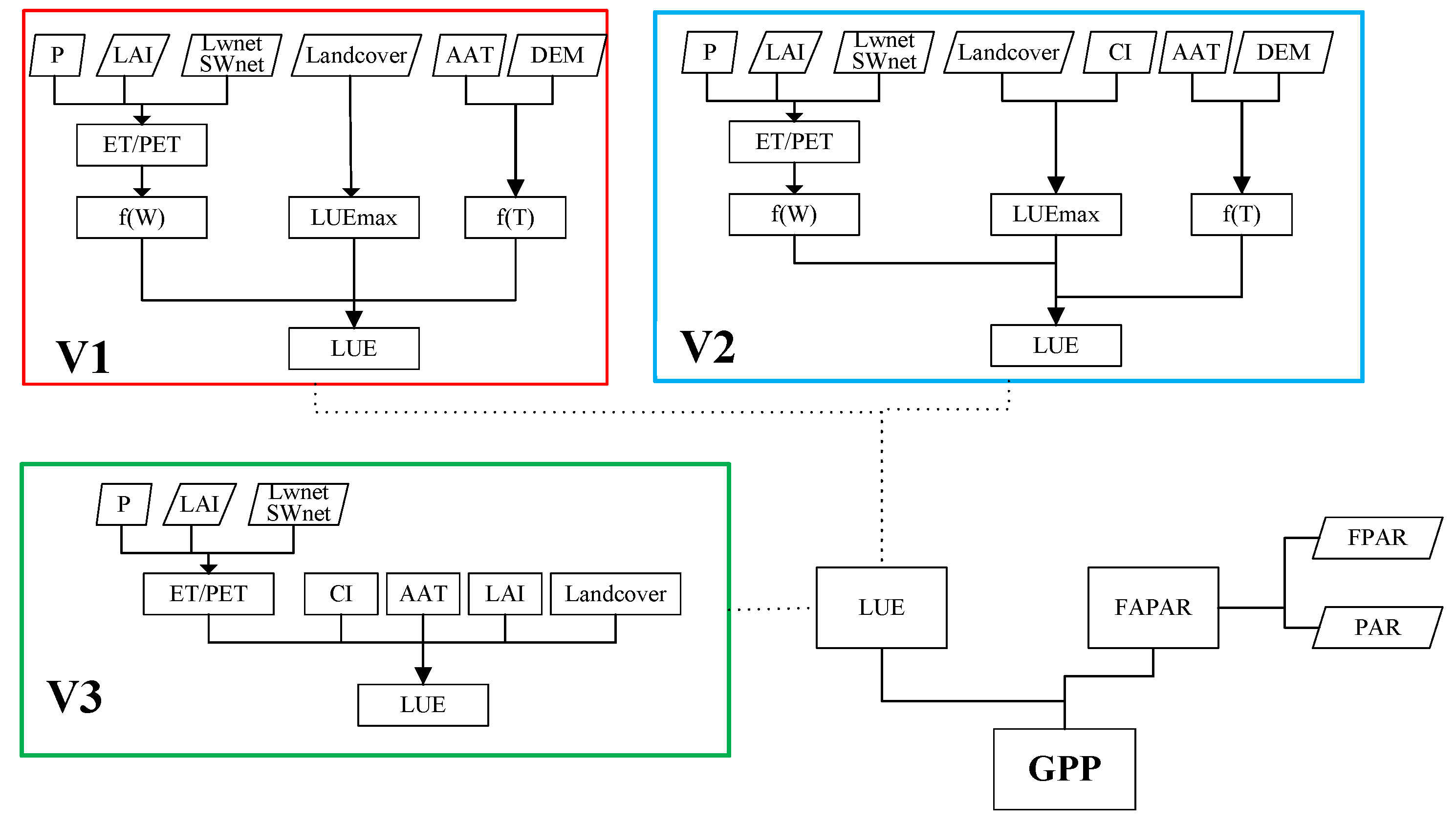
After quality control, 29,056 pieces of FLUXNET site data remained, of which 19,459 pieces were randomly chosen for calibration and the remaining data (9597 pieces) were for validation. Data for the calibration and validation both are globally distributed and cover all vegetation types. Figure 2 shows the validation of the three approaches. We also calculated LUE with MOD17 GPP algorithm [79] and compared with in situ data. The results show that our LUE and GPP products were better than MOD17 results which had lower coefficients of determination (R2) and higher root-mean-square error (RMSE), with R2 of 0.098 for LUE and 0.558 for GPP, and RMSE of 0.545 gC/MJ for LUE and 2.575 gC/m2/d for GPP. The R2 of LUE equaled 0.183 and 0.240 for parameterization approaches V1 and V2, respectively. The RMSE of LUE dropped from 0.508 to 0.487 gC/MJ after considering the CI. The results suggested that the addition of the CI to the parameterization approach slightly improved the accuracy of LUE. The R2 and RMSE of LUE by the Cubist regression approach equaled 0.538 and 0.352 gC/MJ, respectively. In comparison with the former two approaches, the Cubist regression tree approach had great advantages in gaining a higher R2 and a lower RMSE. The three approaches all underestimated LUE, especially when the FLUXNET LUE exceeded 2.0 gC/MJ. However, the underestimation problem was alleviated for GPP, with the R2 ranging from 0.63 to 0.78 and the RMSE ranging from 1.79 to 2.33 gC/m2/d. The LUE in the FLUXNET sites was equal to the GPP in sites divided by the corresponding MODIS FPAR. The uncertainty in the LUE at the sites might result from the error of MODIS FPAR. However, the predicted GPP was calculated by multiplying the FPAR. There was a certain degree of offset of GPP error after multiplication and division operations. In addition, the seasonal variations in solar radiation enhanced the accuracy of GPP estimation.
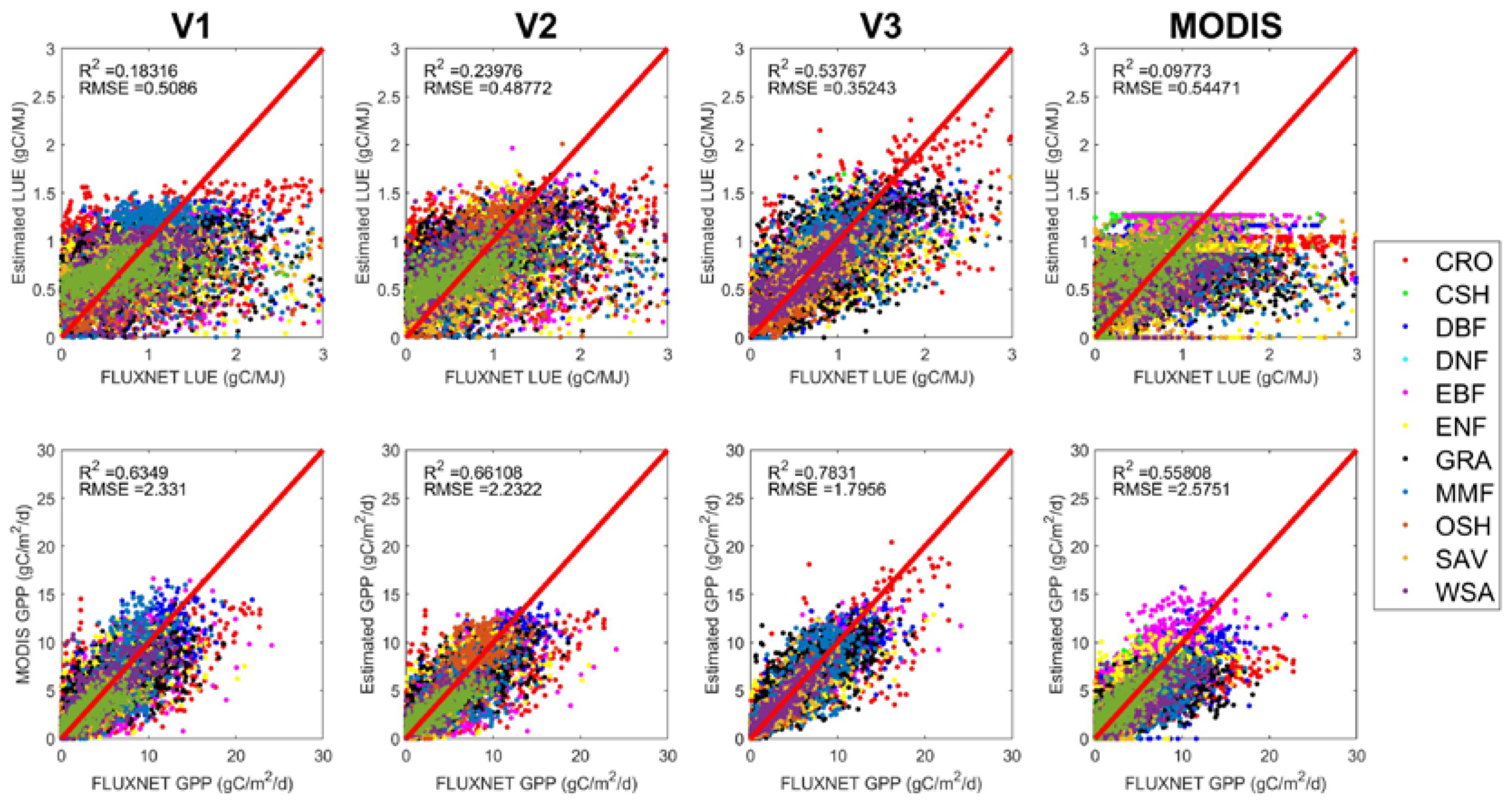
Looking at the validation result in each type of vegetation (Figure 3), it is easy to find that the DBF, GRA and WSA gained high-quality LUE and GPP. In contrast, the two parameterization approaches obtained weak relationships between FLUXNET and estimated LUE in CRO, EBF, MF, CSH and OSH. In CRO, crop species were complicated and might contain C3 plants, C4 plants or both. The different features between C3 and C4 crops [6] introduced errors in CRO. The vegetation in EBF showed few variations in different seasons; therefore, it was difficult to retrieve solid correlations. In addition, EBF was distributed in both high-latitude and low-latitude areas where the maximum LUE and the optimal temperature varied greatly. These factors might lead to the uncertainty in the LUE and GPP in EBF. In MF, OSH and CSH, the main cause was the heterogeneity of plants.
3. Results
3.1. Validation of Global LUE and GPP Results in 2014
We extrapolated the calibrated parameters and models to a global scale and produced LUE and GPP maps for 2014 with a spatial resolution of 5 km and a temporal resolution of 8 days. In this part, we validated the results against FLUXNET measurements. There were 1700 pieces of data observed in 69 sites within 2014. Figure 4 indicates that our LUE and GPP estimates are reliable. The R2 of LUE ranged from 0.21 to 0.30, and the RMSE ranged from 0.41 to 0.55 gC/MJ. The best result was produced by the parameterization approach with the CI, while the least satisfactory one was estimated by the Cubist regression tree model. There were more overestimated LUE values in the Cubist regression approach, some of which reached or even exceeded 3 gC/MJ. Although the Cubist regression tree approach gained the optimum result during calibration, it revealed clear disadvantages in extrapolating to the global scale. Like other empirical methods, the main weakness of Cubist is the vague explanations behind the formulas and the great possibilities to exceed reasonable values when dealing with some rare and special situations. However, it is most likely to obtain pixels that are unsuitable for the estimated relationships when mapping global LUE. Compared with LUE, the accuracy of GPP was improved, with the R2 ranging from 0.51 to 0.60 and the RMSE ranging from 2.42 to 2.87 gC/m2/d. Similarly, the parameterization approach with the CI gained the most satisfactory GPP. Although the Cubist regression tree approach still produced the weakest relationship between estimated GPP and FLUXNET GPP, the overestimation was mitigated because of the constraint of PAR.
Then, we looked at more details in each type of vegetation (Table 3). In DBF, DNF, GRA, MF and WSA, vegetation gained high-quality LUE with R2 values greater than 0.3. In EBF, ENF, OSH and SAV, vegetation obtained acceptable accuracy with R2 values from 0.17 to 0.26. All of the above types of vegetation had RMSE values less than 0.5 gC/MJ. However, all three approaches failed to produce reliable LUE values in CRO, with an R2 less than 0.03 and an RMSE higher than 0.57 gC/MJ. Crop species in CRO were complicated and might contain C3 plants, C4 plants or both. The different features between C3 and C4 crops introduced errors in CRO. In comparison with the parameterization approach without the CI, the parameterization approach with the CI showed clear advantages in all types of vegetation in terms of calculating LUE. In comparison with the Cubist regression tree approach, the parameterization approach with the CI clearly won in CRO, DBF, ENF, GRA, MF, OSH, and SAV and was slightly superior in DNF and obviously inferior in EBF and WSA. Similar to the general situation, the accuracy of GPP was improved in each type of vegetation compared with LUE. The relationship between estimated GPP and FLUXNET GPP was strong, with the R2 values were greater than 0.5 in DBF, DNF, EBF, ENF, GRA, MF, SAV and WSA. However, GPP gained only acceptable accuracy, with R2 values of 0.46 and 0.31 and RMSE values of 2.73 gC/m2/d and 0.86 gC/m2/d in CRO and OSH, respectively. The main errors in OSH were induced by the heterogeneity of plants. The error resources of cropland vegetation will be discussed in Section 4. In general, the parameterization approach with the CI gained the most accurate estimates even though the parameterization approach without the CI surpassed the DNF and the Cubist regression tree approach won in ENF and WSA.
3.2. LUE
3.2.1. Parameterization Approach without the CI
Figure 5 shows the distributions of LUE produced by the parameterization approach without the CI during four periods in 2014. The variations in the four periods indicate that the LUE varied greatly in different seasons. From 2014049 to 2014136, during which spring occurred in the Northern Hemisphere, the LUE in Asia, Europe and North America was generally low, with values less than 1.0 gC/MJ. On these continents, vegetation in coastal areas had a higher LUE than that found in inland areas, even at the same latitude or longitude. In equatorial regions including South America, middle Africa and Southeast Asia, vegetation had the highest LUE, at approximately 1.5 gC/MJ. From the equator to the Southern Hemisphere, LUE decreased to 1.2 gC/MJ at approximately 30° S and then continued to decline to approximately 0.5 gC/MJ in southwestern South America and Africa. The west and south of South America shared low LUE values because of the low temperatures resulting from high altitudes and high latitudes, respectively, while the vegetation in Africa presented a low LUE because of drought [80], which can be supported by the extremely low EF in this study. In Australia, the vegetation had much lower LUE values than those in South America and Africa, with an approximate value of 0.5 gC/MJ, but demonstrated a similar tendency for LUE to increase from the eastern coastline areas, at 1.5 gC/MJ, to the western area, at less than 0.5 gC/MJ, because of the decreasing soil moisture [81].
In the second season (from 2014137 to 2014224), the global vegetation LUE generally illustrated an increasing tendency. During the last two seasons (from 2014225 to 2014365 and from 2014001 to 2014048), the global vegetation LUE showed a gradual decreasing tendency. Vegetation in the Northern Hemisphere had a similar changing trend with that of global vegetation. In eastern North America, Europe and Southeast Asia, the vegetation LUE increased to 1.5 gC/MJ due to the increasing radiation and temperature in the second season, and it declined to approximately 0.8 gC/MJ in the third season; finally, it declined to less than 0.2 gC/MJ in the last season. The Southern Hemisphere, including South America, Africa and Australia, showed fewer changes in LUE distribution during the four different seasons. In the north of Africa and Australia, however, the vegetation illustrated the opposite tendency as that seen in other areas where more radiation induced less LUE because these areas were attacked by drought for the whole year. More radiation causes the temperature to constantly increase, which consequently aggravates the effects of water stress.
3.2.2. Parameterization Approach with CI
Considering the effect of different radiation modes, we added the CI in the parameterization approach and gained a second global LUE distribution (Figure 6). In general, the LUE distributions produced by this approach were similar to those produced by the parameterization approach without the CI; the differences between the two approaches ranged from −0.1 to 0.4 gC/MJ. For example, the differences included the LUE calculated by the second approach (V2) being even higher in high-value zones, which agrees with a previous study that found that diffuse light enhanced LUE within similar environmental conditions [82]. Looking at LUE in every single season, we found (1) from 2014049 to 2014136, the LUE calculated by V2 in South America, middle Africa, and the Southeast Asia reached 1.8 gC/MJ, which was approximately 0.3 gC/MJ more than the LUE calculated by V1. In Europe, the LUE calculated by V2 slightly exceeded that calculated by V1, by 0.1 gC/MJ. On the other hand, the LUE calculated by V2 was lower than the LUE calculated by V1 in the southwestern USA, the north of Africa, and the southwest of Asia; (2) from 2014137 to 2014224, the LUE calculated by V2 in Europe, Canada and northern Asia reached approximately 1.25 gC/MJ and slightly exceeded the LUE calculated by V1 by 0.15 gC/MJ. However, the LUE calculated by V2 was lower than that calculated by V1 in the southwestern USA, the north and south of Africa, the southwest of Asia and the north of Australia; (3) from 2014225 to 2014320, the differences between the two approaches narrowed. Great increases occurred in the north of South America, middle of Africa, and the southeast of Asia. (4) In the last season, variations continuously decreased in the Northern Hemisphere but gradually increased in the Southern Hemisphere, with more areas showing the LUE calculated by V2 being higher than the LUE calculated by V1. In the four seasons, the equatorial regions all showed an increase in LUE as calculated by V2. The main reason is that these areas had abundant rain for the whole year, which reduced the radiation reaching the surface of the earth, consequently leading to a low CI. Therefore, the addition of the CI increased the value of LUE. Other increases in LUE in the region during the growing season can be explained by there being more rain and lower CI.
3.2.3. Cubist Regression Tree Approach
Figure 7 demonstrates the distributions of LUE calculated by the Cubist regression tree approach. Although LUE generally shared a similar distribution with that of the former two approaches, the differences with the parameterization approach without the CI ranged from −0.8 to 0.8 gC/MJ. In general, the positive differences were located in high-latitude areas, while the negative differences were distributed in low-latitude regions. Looking at the LUE on every continent, we found that the southwest of North America had decreases, but other places in North America had increases. The differences diminished in the last season; in South America, few variations were observed; in Europe, the LUE calculated by V3 exceeded that calculated by V1 in the four seasons. In the middle of Africa, the LUE calculated by V3 was higher than that calculated by V1, while the north and south of Africa saw decreases in LUE as calculated by V3. The situation in Asia was more complicated. In northern Asia, including Russia and Mongolia, there were positive differences. During the former three seasons, western Asia and northern China showed negative differences, but the negative differences were eliminated in the last season. Southern China had positive differences in the whole year. There were few variations in the south of Asia. In Australia, except for its southern coastline, the LUE calculated by V3 was lower than the LUE calculated by V1 in the former three seasons, while the negative differences mainly occurred along the southern coastline in the last season.
3.3. GPP
Figure 8 presents the distributions of global annual GPP in 2014. Similar to LUE, there were three equatorial regions, including the northern regions of South America, middle Africa and Southeast Asia, in which vegetation absorbed the most carbon, with GPP greater than 2500 gC/m2/yr. Next to these high carbon sequestration areas, South America, South Africa, South China, India, the coastline of Australia, and some mid-high latitudes in the Northern Hemisphere, such as the eastern USA and Europe, cultivated vegetation with approximately 1500 gC/m2/yr GPP. High-latitude areas, such as Canada and northern Europe, and high-altitude regions, including the USA, the western coastline of South America, the south of Africa, and the Tibetan Plateau of China, saw low carbon sequestration because of the low-temperature stress. Drought-hit areas, such as northern Africa, northern Australia, and Northwest China, also experienced low GPP because of the lack of water.
We compared our 3 GPP results with MODIS GPP (MOD17). The four approaches produced roughly consistent global annual GPP values ranging from 109.23 to 120.65 Pg/yr. The highest value (120.65 Pg/yr) was obtained by the parameterization approach with the CI because this approach considered the different effects between direct and diffuse radiation. The lowest value (109.23 Pg/yr) was estimated by the parameterization approach without the CI. The lands covered by dense vegetation are usually moistened by abundant rain, consequently having a low CI. Therefore, the addition of the CI increased the GPP. We regard this approach as the best method for calculating LUE and GPP. In comparison with the parameterization approach with the CI, the Cubist regression tree approach produced a GPP of 116.41 Pg/yr. This approach divided all pixels into 10 classes and then put them into a corresponding linear rule or rules. The Cubist regression tree approach had little mechanism consideration behind the linear formulas. In addition, 10 rules might not sufficiently satisfy all pixels. Therefore, linear rules are most likely to output negative values. Although we set values to zero in these cases, most were still underestimated. We also plotted the difference between V2 GPP and MODIS GPP (MOD17). It shows that the parameterization approach with the CI gets a higher GPP than MODIS algorithm, especially in the equatorial regions (the northern regions of South America, middle Africa and Southeast Asia) where even more than 600 gC/m2/yr of difference was produced. There were minor differences which means V2 GPP were lower occurred in the south of China, Madagascar islands.
4. Discussion
4.1. Comparison of Three Approaches
4.1.1. Comparison between the Parameterization Approach with and without the CI
To distinguish the different effects of direct and diffuse radiation, we added the CI into the parameterization approach. Figure 4 illustrates the general improvements in LUE and GPP. Typical examples of this improvement can be seen in IT-Isp, AU-Whr, CH-Cha and SE-St1. Table 4 lists more details of these sites. These sites cover the Northern (IT-Isp, CH-Cha, SE-St1) and Southern Hemispheres (AU-Whr) as well as humid (IT-Isp, AU-Whr, CH-Cha) and dry areas (SE-St1). They include 4 types of vegetation: DBF, EBF, GRA and WET.
Figure 9 shows the functions of the CI in the parameterization approach on the LUE estimation. Red dotted lines outline the key points; the 201st and 273rd days in IS-Isp; the 97th and from the 121st to 185th days in AU-Whr; the 113rd, 185th and 273rd days in CH-Cha; and the 73rd and from 209th to 225th days in SE-St1. The CI at these points was less than 0.40, and some values were even below 0.30, which were much lower than the average value of 0.50. In these cases, the accuracy of the parameterization approach with the CI apparently surpassed that without the CI. A lower CI indicates more diffuse radiation, which outputs a higher LUE.
4.1.2. Comparison between Parameterization Approaches and Regression Tree Approach
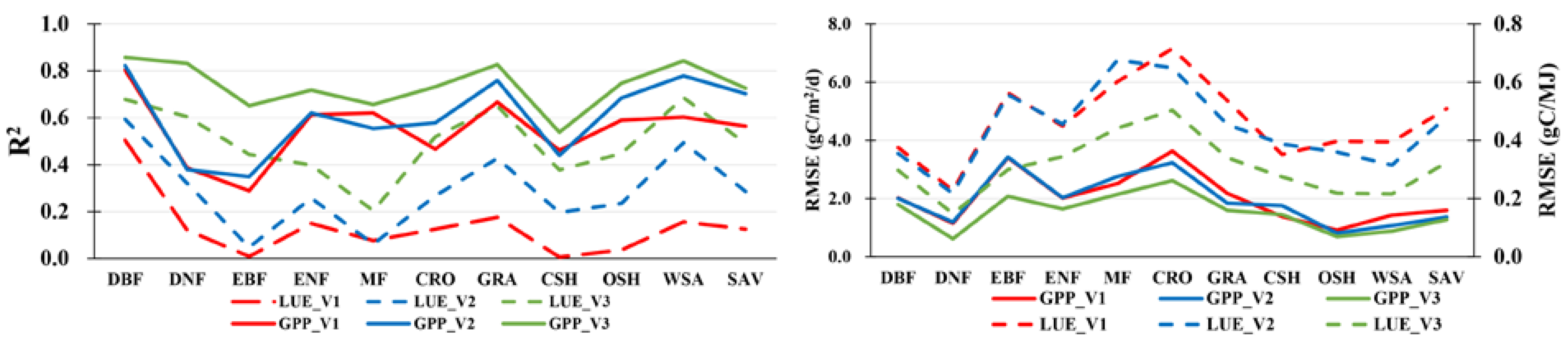
Figure 10 shows the global annual GPP estimated by the three approaches in each type of vegetation. It is easy to find that EBF absorbed the most carbon among all types of vegetation, with a GPP greater than 30 Pg/yr, followed by SAV, WSA, GRA and CRO, with GPP values of approximately 15 Pg/yr. The lowest GPP values were produced by DNF and CSH because of the extremely small areas for DNF and the weak carbon sequestration capacity for CSH. Although the GPP values estimated by the three approaches were similar, there were still some differences for some vegetation types, such as EBF, WSA and GRA. Most of the EBFs were located in equatorial regions with suitable temperature and abundant rain. More rain implied more diffuse radiation; therefore, the clearness index obviously increased the LUE and GPP. Our WSA calibration sites were located in low-latitude areas. The Cubist regression approach was likely to lead to the overestimation when extrapolating this relationship to high-latitude areas (southern Canada, northern USA, Europe and Russia). In contrast, the Cubist regression tree approach underestimated GPP and NPP in GRA because of these inconsistent locations between the calibration sites and land areas.
To analyze the contributions of different latitudes to global vegetation carbon uptake and to compare the performances of the three approaches, we averaged the LUE and summed the annual GPP every 5 km along latitude (Figure 11). In general, LUE demonstrated a tendency of having higher values at lower latitudes and lower values at higher latitudes. In the first season, LUE had its highest value of approximately 1.5 gC/MJ in equatorial regions corresponding to South America, middle Africa and Southeast Asia. There was another important peak near 1.0 gC/MJ at 40°S latitude because of the southern coastal vegetation in Australia. Areas from 50° to 55°S saw higher LUE values, some higher than 1.0 gC/MJ. The curves in the Southern Hemisphere illustrated more fluctuations. The total area of vegetation was much smaller; consequently, the mean LUE was more sensitive to spatial changes. Then, looking at the Northern Hemisphere, it was obvious that vegetation showed a relatively lower LUE, i.e., less than 0.5 gC/MJ, because of the lower temperature and less radiation. The LUE curves calculated by V1 and V2 were more stable than that calculated by V3. The Cubist regression tree approach belongs to the empirical linear regression method, which could be easily affected by a specific parameter and produced a fluctuating line. For the parameterization approaches, the LUE showed a gradual increase from the Arctic to equatorial regions. The three approaches all witnessed a local minimum of 0.5 gC/MJ at 12°N, which was caused by the large area of low LUE in Africa. In the second season, there were few changes (small drops) in the Southern Hemisphere; however, the Northern Hemisphere witnessed large increases up to 1.0 gC/MJ at 50°N. Similar to the first season, the curve generated by V3 showed more fluctuations. In the third season, vegetation in the Southern Hemisphere remained roughly unchanged. However, the LUE in the Northern Hemisphere declined. The peaks produced by V1 and V2 fell to 0.7 gC/MJ, while those produced by V3 remained at 1.0 gC/MJ. In the last season, the Southern Hemisphere saw a slight increase in LUE, with a peak of almost 1.0 gC/MJ. However. The LUE in the Northern Hemisphere went through a slump, and the latitude of the peak moved from 55° to 25°, and the peak LUE declined to 0.5 gC/MJ. Compared with the Southern Hemisphere, the Northern Hemisphere presented much more variation. The main reason for this variation was the distribution of vegetation in the Southern Hemisphere, which was mainly located in low-latitude areas, while the vegetation in the Northern Hemisphere was spread in low- and high-latitude regions. High-latitude areas underwent great changes in temperature and solar radiation, which were essential for vegetation growth. Therefore, the LUE in the Northern Hemisphere varied greatly during different seasons. The two parameterization approaches showed few differences except in equatorial regions and other local maximum values where V2 had a higher LUE than V1. A better explanation for this increase can be found in Section 3.2.2. The Cubist regression tree approach, however, presented a clear difference from the former parameterization approaches. V3 produced a higher LUE in high-latitude areas (50°N and 50°S) and a lower LUE at low-latitude areas (between 30°N and 30°S). Looking at the GPP curves with latitude, there were two clear peaks reaching 75 TgC/yr at 50°N and 130 TgC/yr in equatorial regions. The annual GPP curves from the 3 approaches showed fewer variations than those of LUE.
4.2. Uncertainty Analysis
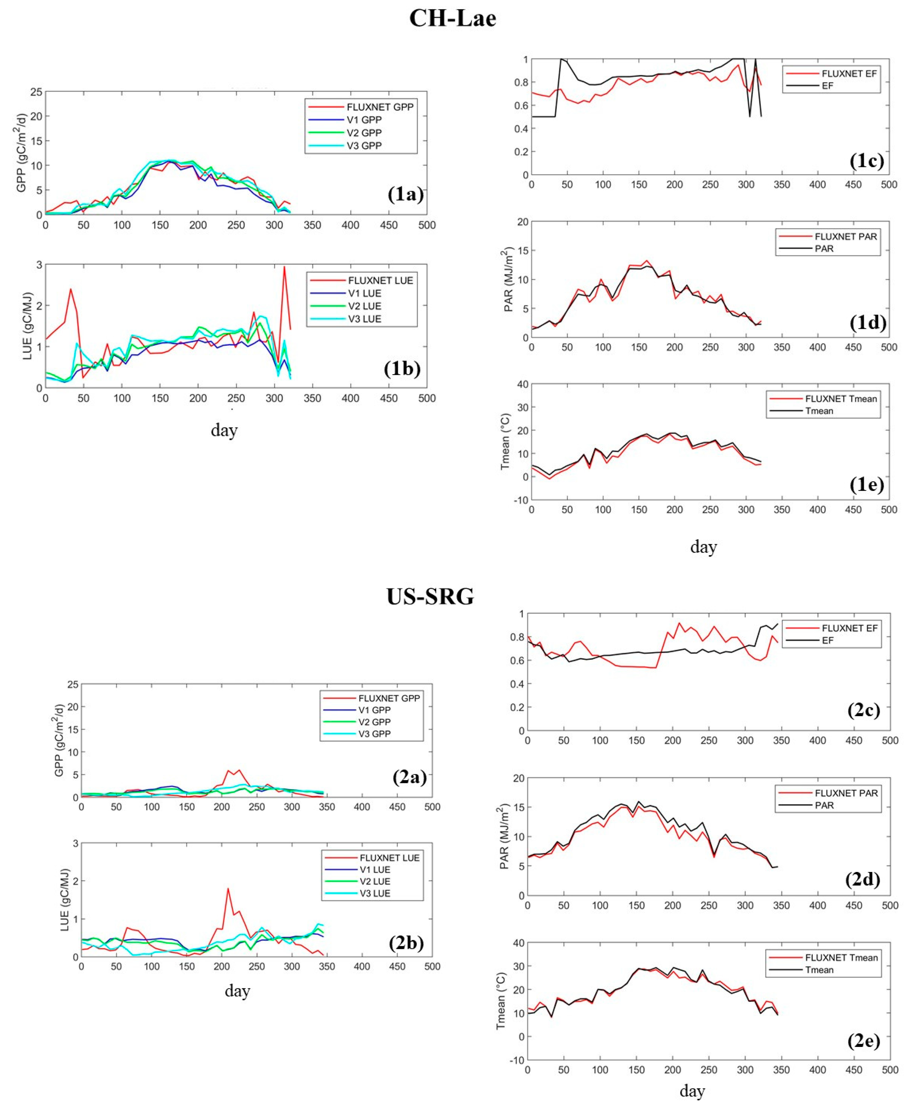
As described in Section 2.2, we used a different dataset for the model calibration and global LUE and GPP estimation. The uncertainty of the input parameters, such as EF, PAR and Tmean, would introduce error to our LUE and GPP products. In this part, we plotted the time series of GPP, LUE, EF, PAR and Tmean in two sites and compared data for calibration and global extrapolation. Figure 12 shows our PAR and Tmean used for global product match well with FLUXNET PAR and Tmean which agrees with the high correlations of them (both higher than 0.95). By contrast, the correlation between FLUXNET EF and global EF is only 0.681, which means EF had higher uncertainty. In CH-Lae, global EF matched well with FLUXNET EF, then we got a satisfactory LUE and GPP, while US-SRG failed to produce either a very good LUE or GPP because of the uncertainty of EF. Therefore, we think EF is a key error source for global LUE and GPP.
4.3. Error Analysis
For most vegetation types, the relationships between FLUXNET and estimated GPP were stronger than LUE. This problem was particularly noticeable in CRO and EBF, with the LUE R2 at less than 0.05 and the GPP R2 at 0.46 and 0.50, respectively. The main causes might come from the process used to calculate LUE. According to Formula (2), the precision of site-scale LUE relies on FLUXNET GPP, incident shortwave (PAR) and MODIS FPAR. We regarded the measured FLUXNET data as reliable; therefore, the uncertainty was mainly decided by FPAR. In some pixels, MODIS FPAR was very low—because of the clouds, inconsistent landcover, or system errors—which would result in an overestimation of LUE. Therefore, the weak relationships between FLUXNET-estimated LUE did not only originate from the error of estimates, but from the FLUXNET LUE.
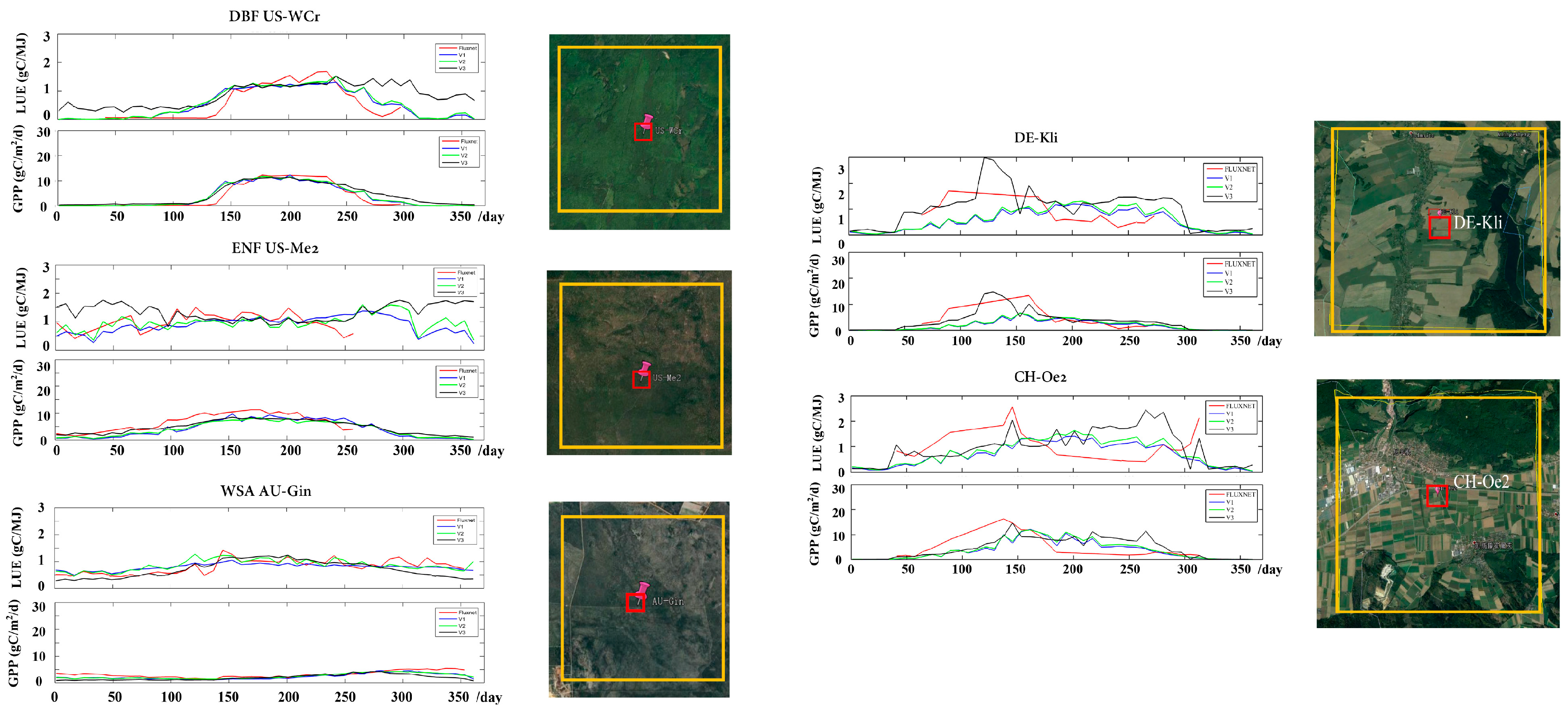
Figure 13 demonstrates the LUE and GPP curves and 5000 m × 5000 m land surface images from a Google map at five sites, with which we can analyze the different effects of homogeneous and heterogeneous land surfaces. US-WCr was covered by DBF, US-Me2 was covered by ENF, AU-Gin was covered by WSA, and DE-Kli and CH-Oe2 were covered by CRO (Table 4). In the former three sites, the land surface was homogeneous within an area of 5000 m × 5000 m. The estimated LUE and GPP curves agreed well with FLUXNET LUE and GPP. However, most sites of croplands were heterogeneous in the same area. DE-Kli and CH-Oe2 showed a single vegetation type in 500 m × 500 m of land. However, they contained different types of vegetation, including croplands, forests, built-up lands and water, in 5000 m × 5000 m areas where the LUE varied greatly [5]. Furthermore, crops could be divided into C3 and C4 plants that produce different LUE [6]. Therefore, the complicated circumstances around croplands resulted in low-quality estimates.
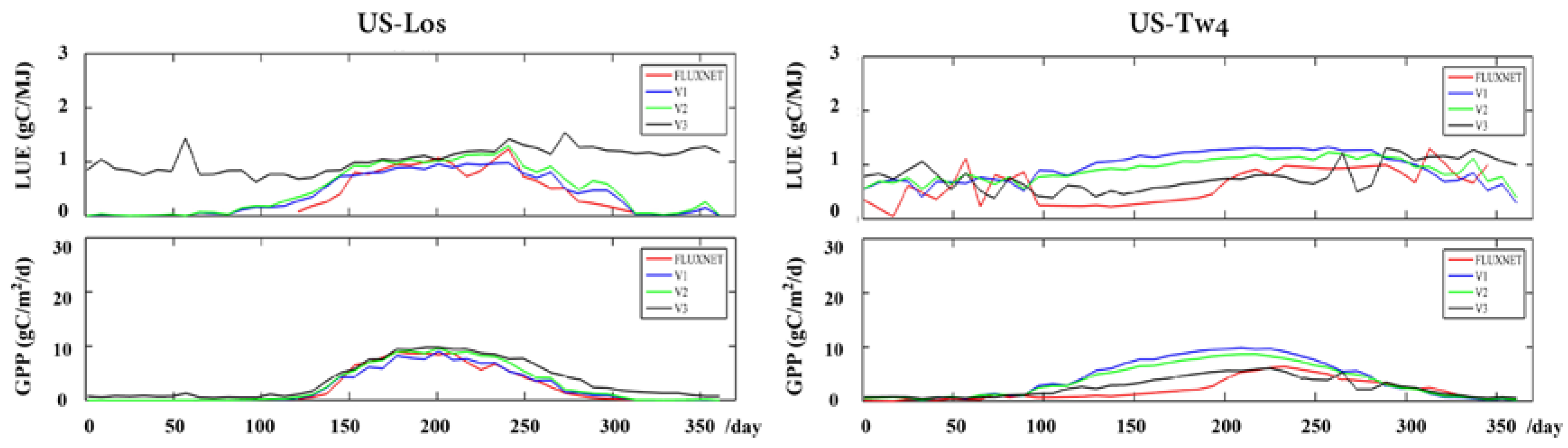
In addition, the misclassification induced errors in the estimated LUE and GPP. We used the MODIS landcover product in this study. Some sites were misclassified, such as US-Los and US-Tw4 (Figure 14), because of inconsistent spatial resolutions and classification errors. These two sites were recorded as grassland in the FLUXNET dataset, while the corresponding pixel was cropland in the MODIS landcover data. In the parameterization approaches, we set different maximum LUEs for each vegetation type. These pixels were wrongly treated as cropland rather than grassland, in which the maximum LUE was lower than the former. Consequently, the LUE and GPP were overestimated.
5. Conclusions
In this study, we collected discrete FLUXNET eddy-covariance and meteorological data and spatially continuous MODIS, GLASS and ERA-Interim data to estimate the global LUE and GPP. The SCE-UA optimization method had a high efficiency of solving the global optimal solution under nonlinear constraints and never depended on the initial value of the mode, and the Cubist regression tree approach provided a powerful tool with which to upscale site-observed fluxes to a larger scale with satellite-derived parameters and other explanatory variables. We established three LUE-based GPP approaches to assess the different performances at both the site and the global scales. The method of obtaining the LUE was based on (1) a parameterization approach without the CI, (2) a parameterization approach with the CI, and (3) a Cubist regression tree approach.
By validating with FLUXNET measurements at the site scale, we obtained the following:
(1) The Cubist regression approach performed better than the parameterization approaches in estimating LUE and GPP.
(2) The three approaches all underestimated the LUE, especially when the FLUXNET LUE exceeded 2.0 gC/MJ. However, the underestimation problem was alleviated for GPP.
However, when applying these models to the global LUE and GPP in 2014, we found the following:
(1) The LUE and GPP estimated by the three approaches were reliable, of which the parameterization approach with the CI produced the most satisfactory result then closely followed by the parameterization approach without the CI, while the Cubist regression approach produced the least satisfactory result.
(2) The accuracy of GPP was higher than that of LUE for all types of vegetation.
(3) The LUE distributions showed some variations in different seasons, but vegetation had the highest LUE at approximately 1.5 gC/MJ for the entire year in equatorial regions (South America, middle Africa and Southeast Asia).
(4) The three approaches produced roughly consistent global annual GPP values, ranging from 109.23 to 120.65 Pg/yr.
In conclusion, our results suggest the parameterization approaches are robust when extrapolating to the global scale, of which the parameterization approach with CI performs slightly better than that without CI. By contrast, the Cubist regression tree produced LUE and GPP with lower accuracy even though it performed the best for model validation at the site scale.
Author Contributions
M.W. and R.S. conceived and designed the work; M.W. analyzed the data and wrote the manuscript, R.S. provided ideas and modified the manuscript; A.Z. processed some experimental data. Z.X. provided data and suggestions. All authors have read and agreed to the published version of the manuscript.
Funding
This work was supported by the National Key R&D Program of China (2017YFA0603002, 2016YFB0501502) and the National Natural Science Foundation of China (41531174).
Acknowledgments
The data used in this paper include Fluxnet2015 dataset, MODIS GPP/NPP products (MOD17A3 and MOD17A2). We sincerely thank all contributors of the data. We thank all the reviewers for their careful reading of the manuscript and their constructive remarks.
Conflicts of Interest
The authors declare no conflict of interest.
References
- Running, S.W.; Baldocchi, D.; Turner, D.; Gower, S.T.; Bakwin, P.; Hibbard, K. A global terrestrial monitoring network integrating tower fluxes, flask sampling, ecosystem modeling and EOS satellite data. Remote Sens. Environ. 1999, 70, 108–127. [Google Scholar] [CrossRef]
- Tramontana, G.; Ichii, K.; Camps-Valls, G.; Tomelleri, E.; Papale, D. Uncertainty analysis of gross primary production upscaling using Random Forests, remote sensing and eddy covariance data. Remote Sen. Environ. 2015, 168, 360–373. [Google Scholar] [CrossRef]
- McCallum, I.; Franklin, O.; Moltchanova, E.V.; Merbold, L.; Schmullius, C.; Shvidenko, A.; Schepaschenko, D.; Fritz, S. Improved light and temperature responses for light-use-efficiency-based GPP models. Biogeosciences 2013, 10, 6577–6590. [Google Scholar] [CrossRef] [Green Version]
- He, L.; Chen, J.M.; Liu, J.; Bélair, S.; Luo, X. Assessment of SMAP soil moisture for global simulation of gross primary production. J. Geophys. Res. 2017, 122, 1549–1563. [Google Scholar] [CrossRef]
- Fletcher, B.J.; Gornall, J.L.; Poyatos, R.; Press, M.C.; Stoy, P.C.; Huntley, B.; Baxter, R.; Phoenix, G.K. Photosynthesis and productivity in heterogeneous arctic tundra: Consequences for ecosystem function of mixing vegetation types at stand edges. J. Ecol. 2012, 100, 441–451. [Google Scholar] [CrossRef] [Green Version]
- Liu, L.; Guan, L.; Liu, X. Directly estimating diurnal changes in GPP for C3 and C4 crops using far-red sun-induced chlorophyll fluorescence. Agric. For. Meteorol. 2017, 232, 1–9. [Google Scholar]
- Missik, J.; Benson, M.C.; Oishi, A.C.; Novick, K.A.; Miniat, C. Quantifying Age-Related Hydraulic and Biochemical Constraints on Tree Photosynthesis in the Southern Appalachian Mountains. In Proceedings of the Agu Fall Meeting, San Francisco, CA, USA, 14–18 December 2015. [Google Scholar]
- Wang, S.; Ibrom, A.; Bauer-Gottwein, P.; Garcia, M. Incorporating diffuse radiation into a light use efficiency and evapotranspiration model: An 11-year study in a high latitude deciduous forest. Agric. For. Meteorol. 2018, 248, 479–493. [Google Scholar] [CrossRef] [Green Version]
- Cramer, W.; Kicklighter, D.W.; Bondeau, A.; Iii, B.M.; Churkina, G.; Nemry, B.; Ruimy, A.; Schloss, A.L.; Intercomparison, T.P. Comparing global models of terrestrial net primary productivity (NPP): Overview and key results. Glob. Chang. Biol. 1999, 5, 1–15. [Google Scholar] [CrossRef]
- Zhang, Y.; Song, C.; Sun, G.; Band, L.E.; McNulty, S.; Noormets, A.; Zhang, Q.; Zhang, Z. Development of a coupled carbon and water model for estimating global gross primary productivity and evapotranspiration based on eddy flux and remote sensing data. Agric. For. Meteorol. 2016, 223, 116–131. [Google Scholar] [CrossRef] [Green Version]
- Running, S.W.; Nemani, R.R.; Heinsch, F.A.; Zhao, M.; Reeves, M.; Hashimoto, H. A continuous satellite-derived measure of global terrestrial primary production. Bioscience 2004, 54, 547–560. [Google Scholar] [CrossRef]
- Yuan, W.; Liu, S.; Yu, G.; Bonnefond, J.-M.; Chen, J.; Davis, K.; Desai, A.R.; Goldstein, A.H.; Gianelle, D.; Rossi, F. Global estimates of evapotranspiration and gross primary production based on MODIS and global meteorology data. Remote Sens. Environ. 2010, 114, 1416–1431. [Google Scholar] [CrossRef] [Green Version]
- Chen, J.M.; Mo, G.; Pisek, J.; Liu, J.; Deng, F.; Ishizawa, M.; Chan, D. Effects of foliage clumping on the estimation of global terrestrial gross primary productivity. Glob. Biogeochem. Cycles 2012, 26. [Google Scholar] [CrossRef]
- Christian, B.; Markus, R.; Enrico, T.; Philippe, C.; Martin, J.; Nuno, C.; Christian, R.D.; M Altaf, A.; Dennis, B.; Bonan, G.B. Terrestrial gross carbon dioxide uptake: Global distribution and covariation with climate. Science 2010, 329, 834–838. [Google Scholar]
- Dan, L.; Wenwen, C.; Jiangzhou, X.; Wenjie, D.; Guangsheng, Z.; Yang, C.; Haicheng, Z.; Wenping, Y. Global validation of a process-based model on vegetation gross primary production using eddy covariance observations. PLoS ONE 2014, 9, e110407. [Google Scholar]
- Anav, A.; Friedlingstein, P.; Beer, C.; Ciais, P.; Harper, A.; Jones, C.; Murray-Tortarolo, G.; Papale, D.; Parazoo, N.C.; Peylin, P. Spatio-temporal patterns of terrestrial gross primary production: A review. Rev. Geophys. 2015, 53, 785–818. [Google Scholar] [CrossRef] [Green Version]
- Maosheng, Z.; Running, S.W. Drought-induced reduction in global terrestrial net primary production from 2000 through 2009. Science 2010, 329, 940. [Google Scholar]
- Pan, S.; Tian, H.; Dangal, S.R.S.; Ouyang, Z.; Chaoqun, L.U.; Yang, J.; Tao, B. Impacts of climate variability and extremes on global net primary production in the first decade of the 21st century. J. Geogr. Sci. 2015, 25, 1027–1044. [Google Scholar] [CrossRef]
- Xiao, X.; Zhang, Q.; Braswell, B.; Urbanski, S.; Boles, S.; Wofsy, S.; Moore III, B.; Ojima, D. Modeling gross primary production of temperate deciduous broadleaf forest using satellite images and climate data. Remote Sens. Environ. 2004, 91, 256–270. [Google Scholar] [CrossRef]
- Wu, C.; Chen, J.M.; Huang, N. Predicting gross primary production from the enhanced vegetation index and photosynthetically active radiation: Evaluation and calibration. Remote Sens. Environ. 2011, 115, 3424–3435. [Google Scholar] [CrossRef]
- Shi, H.; Li, L.; Eamus, D.; Huete, A.; Cleverly, J.; Tian, X.; Yu, Q.; Wang, S.; Montagnani, L.; Magliulo, V. Assessing the ability of MODIS EVI to estimate terrestrial ecosystem gross primary production of multiple land cover types. Ecol. Indic. 2017, 72, 153–164. [Google Scholar] [CrossRef] [Green Version]
- Monteith, J.L. Climate and the efficiency of crop production in Britain. Philos. Trans. R. Soc. Lond. B Biol. Sci. 1977, 281, 277–294. [Google Scholar]
- Monteith, J. Solar radiation and productivity in tropical ecosystems. J. Appl. Ecol. 1972, 9, 747–766. [Google Scholar] [CrossRef] [Green Version]
- Running, S.W.; Thornton, P.E.; Nemani, R.; Glassy, J.M. Global Terrestrial Gross and Net Primary Productivity from the Earth Observing System. In Methods in Ecosystem Science; Springer: Berlin/Heidelberg, Germany, 2000; pp. 44–57. [Google Scholar]
- Wu, C.Y.; Munger, J.W.; Niu, Z.; Kuang, D. Comparison of multiple models for estimating gross primary production using MODIS and eddy covariance data in Harvard Forest. Remote Sens. Environ. 2010, 114, 2925–2939. [Google Scholar] [CrossRef]
- Mäkelä, A.; Pulkkinen, M.; Kolari, P.; Lagergren, F.; Berbigier, P.; Lindroth, A.; Loustau, D.; Nikinmaa, E.; Vesala, T.; Hari, P. Developing an empirical model of stand GPP with the LUE approach: Analysis of eddy covariance data at five contrasting conifer sites in Europe. Glob. Chang. Biol. 2008, 14, 92–108. [Google Scholar] [CrossRef]
- McCallum, I.; Wagner, W.; Schmullius, C.; Shvidenko, A.; Obersteiner, M.; Fritz, S.; Nilsson, S. Satellite-based terrestrial production efficiency modeling. Carbon Balance Manag. 2009, 4, 8. [Google Scholar] [CrossRef] [Green Version]
- Yuan, W.; Liu, S.; Zhou, G.; Zhou, G.; Tieszen, L.L.; Baldocchi, D.; Bernhofer, C.; Gholz, H.; Goldstein, A.H.; Goulden, M.L. Deriving a light use efficiency model from eddy covariance flux data for predicting daily gross primary production across biomes. Agric. For. Meteorol. 2007, 143, 189–207. [Google Scholar] [CrossRef] [Green Version]
- Wang, H.; Jia, G.; Fu, C.; Feng, J.; Zhao, T.; Ma, Z. Deriving maximal light use efficiency from coordinated flux measurements and satellite data for regional gross primary production modeling. Remote Sens. Environ. 2010, 114, 2248–2258. [Google Scholar] [CrossRef]
- Norman, J.; Anderson, M.; Diak, G. An approach for mapping light-use efficiency on regional scales using satellite observations. In Proceedings of the 1996 International Geoscience and Remote Sensing Symposium, Lincoln, NE, USA, 27–31 May 1996; pp. 2358–2360. [Google Scholar]
- Gamon, J.A.; Bond, B. Effects of irradiance and photosynthetic downregulation on the photochemical reflectance index in Douglas-fir and ponderosa pine. Remote Sens. Environ. 2013, 135, 141–149. [Google Scholar] [CrossRef]
- Castro, S.; Sanchez-Azofeifa, A. Testing of Automated Photochemical Reflectance Index Sensors as Proxy Measurements of Light Use Efficiency in an Aspen Forest. Sensors 2018, 18, 3302. [Google Scholar] [CrossRef] [Green Version]
- Hmimina, G.; Merlier, E.; Dufrene, E.; Soudani, K. Deconvolution of pigment and physiologically related photochemical reflectance index variability at the canopy scale over an entire growing season. Plant Cell Environ. 2015, 38, 1578–1590. [Google Scholar] [CrossRef] [PubMed]
- Merlier, E.; Hmimina, G.; Dufrene, E.; Soudani, K. Explaining the variability of the photochemical reflectance index (PRI) at the canopy-scale: Disentangling the effects of phenological and physiological changes. J. Photochem. Photobiol. B-Biol. 2015, 151, 161–171. [Google Scholar] [CrossRef] [PubMed]
- Zhang, Q.; Ju, W.; Chen, J.; Wang, H.; Yang, F.; Fan, W.; Huang, Q.; Zheng, T.; Feng, Y.; Zhou, Y.; et al. Ability of the Photochemical Reflectance Index to Track Light Use Efficiency for a Sub-Tropical Planted Coniferous Forest. Remote Sens. 2015, 7, 16938–16962. [Google Scholar] [CrossRef] [Green Version]
- Porcar-Castell, A.; Garcia-Plazaola, J.I.; Nichol, C.J.; Kolari, P.; Olascoaga, B.; Kuusinen, N.; Fernandez-Marin, B.; Pulkkinen, M.; Juurola, E.; Nikinmaa, E. Physiology of the seasonal relationship between the photochemical reflectance index and photosynthetic light use efficiency. Oecologia 2012, 170, 313–323. [Google Scholar] [CrossRef] [PubMed]
- Ma, X.; Huete, A.; Yu, Q.; Restrepo-Coupe, N.; Beringer, J.; Hutley, L.B.; Kanniah, K.D.; Cleverly, J.; Eamus, D. Parameterization of an ecosystem light-use-efficiency model for predicting savanna GPP using MODIS EVI. Remote Sens. Environ. 2014, 154, 253–271. [Google Scholar] [CrossRef]
- Wei, S.; Yi, C.; Fang, W.; Hendrey, G. A global study of GPP focusing on light-use efficiency in a random forest regression model. Ecosphere 2017, 8, e01724. [Google Scholar] [CrossRef]
- Horn, J.E.; Schulz, K. Spatial extrapolation of light use efficiency model parameters to predict gross primary production. J. Adv. Model. Earth Syst. 2011, 3. [Google Scholar] [CrossRef]
- Zhang, Y.L.; Song, C.H.; Sun, G.; Band, L.E.; Noormets, A.; Zhang, Q.F. Understanding moisture stress on light use efficiency across terrestrial ecosystems based on global flux and remote-sensing data. J. Geophys. Res. Biogeosci. 2015, 120, 2053–2066. [Google Scholar] [CrossRef]
- Xin, Q.C.; Gong, P.; Suyker, A.E.; Si, Y.L. Effects of the partitioning of diffuse and direct solar radiation on satellite-based modeling of crop gross primary production. Int. J. Appl. Earth Obs. Geoinf. 2016, 50, 51–63. [Google Scholar] [CrossRef]
- He, M.Z.; Ju, W.M.; Zhou, Y.L.; Chen, J.M.; He, H.L.; Wang, S.Q.; Wang, H.M.; Guan, D.X.; Yan, J.H.; Li, Y.N.; et al. Development of a two-leaf light use efficiency model for improving the calculation of terrestrial gross primary productivity. Agric. For. Meteorol. 2013, 173, 28–39. [Google Scholar] [CrossRef]
- Xie, X.; Li, A.; Jin, H.; Yin, G.; Nan, X. Derivation of temporally continuous leaf maximum carboxylation rate (V-cmax) from the sunlit leaf gross photosynthesis productivity through combining BEPS model with light response curve at tower flux sites. Agric. For. Meteorol. 2018, 259, 82–94. [Google Scholar] [CrossRef]
- Zheng, T.; Chen, J.M. Photochemical reflectance ratio for tracking light use efficiency for sunlit leaves in two forest types. Isprs J. Photogramm. Remote Sens. 2017, 123, 47–61. [Google Scholar] [CrossRef]
- Zhou, Y.L.; Hilker, T.; Ju, W.M.; Coops, N.C.; Black, T.A.; Chen, J.M.; Wu, X.C. Modeling Gross Primary Production for Sunlit and Shaded Canopies Across an Evergreen and a Deciduous Site in Canada. IEEE Trans. Geosci. Remote Sens. 2017, 55, 1859–1873. [Google Scholar] [CrossRef]
- Kumar, R.; Umanand, L. Estimation of global radiation using clearness index model for sizing photovoltaic system. Renew. Energy 2005, 30, 2221–2233. [Google Scholar] [CrossRef]
- Zhou, J.; Li, E.; Wei, H.; Li, C.; Qiao, Q.; Armaghani, D.J. Random forests and cubist algorithms for predicting shear strengths of rockfill materials. Appl. Sci. 2019, 9, 1621. [Google Scholar] [CrossRef] [Green Version]
- Noi, P.T.; Degener, J.; Kappas, M. Comparison of multiple linear regression, cubist regression, and random forest algorithms to estimate daily air surface temperature from dynamic combinations of MODIS LST data. Remote Sens. 2017, 9, 398. [Google Scholar] [CrossRef] [Green Version]
- Houborg, R.; McCabe, M.F. A hybrid training approach for leaf area index estimation via Cubist and random forests machine-learning. ISPRS J. Photogramm. Remote Sens. 2018, 135, 173–188. [Google Scholar] [CrossRef]
- Hilker, T.; Coops, N.C.; Schwalm, C.R.; Jassal, R.S.; Black, T.A.; Krishnan, P. Effects of mutual shading of tree crowns on prediction of photosynthetic light-use efficiency in a coastal Douglas-fir forest. Tree phys. 2008, 28, 825–834. [Google Scholar] [CrossRef]
- Schubert, P.; Lagergren, F.; Aurela, M.; Christensen, T.; Grelle, A.; Heliasz, M.; Klemedtsson, L.; Lindroth, A.; Pilegaard, K.; Vesala, T.; et al. Modeling GPP in the Nordic forest landscape with MODIS time series data—Comparison with the MODIS GPP product. Remote Sens. Environ. 2012, 126, 136–147. [Google Scholar] [CrossRef]
- Xiao, J.; Zhuang, Q.; Law, B.E.; Chen, J.; Baldocchi, D.D.; Cook, D.R.; Oren, R.; Richardson, A.D.; Wharton, S.; Ma, S. A continuous measure of gross primary production for the conterminous United States derived from MODIS and AmeriFlux data. Remote Sens. Environ. 2010, 114, 576–591. [Google Scholar] [CrossRef] [Green Version]
- Boyte, S.P.; Wylie, B.K.; Howard, D.M.; Dahal, D.; Gilmanov, T. Estimating carbon and showing impacts of drought using satellite data in regression-tree models. Int. J. Remote Sens. 2017, 39, 374–398. [Google Scholar] [CrossRef]
- McCree, K.J. Test of current definitions of photosynthetically active radiation against leaf photosynthesis data. Agric. Meteorol. 1972, 10, 443–453. [Google Scholar] [CrossRef]
- Vermote, E.F.; El Saleous, N.; Justice, C.O.; Kaufman, Y.J.; Privette, J.L.; Remer, L.; Roger, J.C.; Tanré, D. Atmospheric correction of visible to middle-infrared EOS-MODIS data over land surfaces: Background, operational algorithm and validation. J. Geophys. Res. Atmos. 1997, 102, 17131–17141. [Google Scholar] [CrossRef] [Green Version]
- Vermote, E.F.; Saleous, E.L.; Nazmi, Z.; Christopher, O. Atmospheric correction of MODIS data in the visible to middle infrared: First results. Remote Sens. Environ. 2002, 83, 97–111. [Google Scholar] [CrossRef]
- Liang, S.; Fang, H.; Chen, M.; Shuey, C.J.; Walthall, C.; Daughtry, C.; Morisette, J.; Schaaf, C.; Strahler, A. Validating MODIS land surface reflectance and albedo products: Methods and preliminary results. Remote Sens. Environ. 2002, 83, 149–162. [Google Scholar] [CrossRef]
- Chen, J.M.; Feng, D.; Mingzhen, C. Locally adjusted cubic-spline capping for reconstructing seasonal trajectories of a satellite-derived surface parameter. IEEE Trans. Geosci. Remote Sens. 2006, 44, 2230–2238. [Google Scholar] [CrossRef]
- Zhao, M.; Heinsch, F.A.; Nemani, R.R.; Running, S.W. Improvements of the MODIS terrestrial gross and net primary production global data set. Remote Sens. Environ. 2005, 95, 164–176. [Google Scholar] [CrossRef]
- Liang, S.; Zhao, X.; Liu, S.; Yuan, W.; Cheng, X.; Xiao, Z.; Zhang, X.; Liu, Q.; Cheng, J.; Tang, H.; et al. A long-term Global LAnd Surface Satellite (GLASS) data-set for environmental studies. Int. J. Digit. Earth 2013, 6, 5–33. [Google Scholar] [CrossRef]
- Xiao, Z.; Liang, S.; Sun, R. Evaluation of Three Long Time Series for Global Fraction of Absorbed Photosynthetically Active Radiation (FAPAR) Products. IEEE Trans. Geosci. Remote Sens. 2018, 56, 5509–5524. [Google Scholar] [CrossRef]
- Yan, K.; Park, T.; Yan, G.; Liu, Z.; Yang, B.; Chen, C.; Nemani, R.; Knyazikhin, Y.; Myneni, R. Evaluation of MODIS LAI/FPAR Product Collection 6. Part 2: Validation and Intercomparison. Remote Sens. 2016, 8, 460. [Google Scholar] [CrossRef] [Green Version]
- Liang, S.; Zhang, X.; Xiao, Z.; Cheng, J.; Liu, Q.; Zhao, X. Global LAnd Surface Satellite (GLASS) Products: Algorithms, Validation and Analysis; Springer Science & Business Media: Berlin/Heidelberg, Germany, 2013. [Google Scholar]
- Balsamo, G.; Albergel, C.; Beljaars, A.; Boussetta, S.; Brun, E.; Cloke, H.; Dee, D.; Dutra, E.; Muñoz-Sabater, J.; Pappenberger, F.; et al. ERA-Interim/Land: A global land surface reanalysis data set. Hydrol. Earth Syst. Sci. 2015, 19, 389–407. [Google Scholar] [CrossRef] [Green Version]
- Potter, C.S.; Randerson, J.T.; Field, C.B.; Matson, P.A.; Vitousek, P.M.; Mooney, H.A.; Klooster, S.A. Terrestrial ecosystem production: A process model based on global satellite and surface data. Glob. Biogeochem. Cycles 1993, 7, 811–841. [Google Scholar] [CrossRef]
- Zhang, K.; Kimball, J.S.; Nemani, R.R.; Running, S.W. A continuous satellite-derived global record of land surface evapotranspiration from 1983 to 2006. Water Resour. Res. 2010, 46, 109–118. [Google Scholar] [CrossRef] [Green Version]
- Chen, Q.; Rui, S.; Xu, Z.; Lei, Z.; Liu, L.; Hao, L.; Jiang, G. A Study of Shelterbelt Transpiration and Cropland Evapotranspiration in an Irrigated Area in the Middle Reaches of the Heihe River in Northwestern China. IEEE Geosci. Remote Sens. Lett. 2015, 12, 369–373. [Google Scholar]
- Zhang, K.; Kimball, J.S.; Mu, Q.; Jones, L.A.; Goetz, S.J.; Running, S.W. Satellite based analysis of northern ET trends and associated changes in the regional water balance from 1983 to 2005. J. Hydrol. 2009, 379, 92–110. [Google Scholar] [CrossRef]
- Priestley, C.H.; Taylor, R.J. On the assessment of surface heat flux and evaporation using large-scale parameters. Mon. Weather Rev. 1972, 100, 81–92. [Google Scholar]
- Cui, T.; Wang, Y.; Sun, R.; Qiao, C.; Fan, W.; Jiang, G.; Hao, L.; Zhang, L. Estimating Vegetation Primary Production in the Heihe River Basin of China with Multi-Source and Multi-Scale Data. PLoS ONE 2016, 11, e0153971. [Google Scholar] [CrossRef] [Green Version]
- Duan, Q.Y.; Gupta, V.K.; Sorooshian, S. Shuffled complex evolution approach for effective and efficient global minimization. J. Optim. Theory Appl. 1993, 76, 501–521. [Google Scholar]
- Jiang, Z.; Chen, Z.; Ren, J.; Huang, Q. Inversion of winter wheat leaf area index based on canopy reflectance model and HJ CCD image. In Proceedings of the Second International Conference on Agro-geoinformatics, Fairfax, VA, USA, 12–16 August 2013. [Google Scholar]
- Gupta, V.K. Optimal Use of the SCE-UA Global Optimization Method for Calibrating Watershed Models. J. Hydrol. 1994, 158, 265–284. [Google Scholar]
- Kan, G.; He, X.; Ding, L.; Li, J.; Liang, K.; Hong, Y. A heterogeneous computing accelerated SCE-UA global optimization method using OpenMP, OpenCL, CUDA, and OpenACC. Water Sci. Technol. 2017, 76, 1640–1651. [Google Scholar]
- Jeon, J.H.; Park, C.G.; Engel, B.A. Comparison of Performance between Genetic Algorithm and SCE-UA for Calibration of SCS-CN Surface Runoff Simulation. Water 2014, 6, 3433–3456. [Google Scholar] [CrossRef] [Green Version]
- Huijuna, X.U.; Chen, Y.; Zeng, B.; Jinxianga, H.E.; Liao, Z. Application of SCE-UA Algorithm to Parameter Optimization of Liuxihe Model. Trop. Geogr. 2012, 32, 32–37. [Google Scholar]
- Song, X.; Zhan, C.; Xia, J. Integration of a statistical emulator approach with the SCE-UA method for parameter optimization of a hydrological model. Sci. Bull. 2012, 57, 3397–3403. [Google Scholar] [CrossRef] [Green Version]
- Kuhn, M.; Johnson, K. Regression trees and rule-based models. In Applied Predictive Modeling; Springer: Berlin/Heidelberg, Germany, 2013; pp. 173–220. [Google Scholar]
- Running, S.W.; Zhao, M. Daily GPP and annual NPP (MOD17A2/A3) products NASA Earth Observing System MODIS land algorithm. 2015. Available online: https://www.ntsg.umt.edu/files/modis/MOD17UsersGuide2015_v3.pdf (accessed on 15 March 2020).
- Hoffman, M.T.; Carrick, P.; Gillson, L.; West, A. Drought, climate change and vegetation response in the succulent karoo, South Africa. S. Afr. J. Sci. 2009, 105, 54–60. [Google Scholar] [CrossRef]
- Carrao, H.; Naumann, G.; Barbosa, P. Mapping global patterns of drought risk: An empirical framework based on sub-national estimates of hazard, exposure and vulnerability. Glob. Environ. Chang. 2016, 39, 108–124. [Google Scholar] [CrossRef]
- Kanniah, K.D.; Beringer, J.; Hutley, L. Exploring the link between clouds, radiation, and canopy productivity of tropical savannas. Agric. Forest Meteorol. 2013, 182, 304–313. [Google Scholar] [CrossRef]
Figure 1.
The flow chart of global Light use efficiency (LUE) and gross primary productivity (GPP) by 3 approaches.
Figure 1.
The flow chart of global Light use efficiency (LUE) and gross primary productivity (GPP) by 3 approaches.

Figure 2.
The validation results of 3 approaches. Approach V1: Parameterization approach without the clearness index (CI); Approach V2: Parameterization approach with the CI; Approach V3: Cubist regression tree approach; MODIS: MODIS 17 algorithm.
Figure 2.
The validation results of 3 approaches. Approach V1: Parameterization approach without the clearness index (CI); Approach V2: Parameterization approach with the CI; Approach V3: Cubist regression tree approach; MODIS: MODIS 17 algorithm.

Figure 3.
The accuracy of 3 approaches in each type of vegetation. V1: Parameterization approach without the CI; V2: Parameterization approach with the CI; V3: Cubist regression tree approach.
Figure 3.
The accuracy of 3 approaches in each type of vegetation. V1: Parameterization approach without the CI; V2: Parameterization approach with the CI; V3: Cubist regression tree approach.

Figure 4.
LUE and GPP validation. V1: Parameterization approach without the CI; V2: Parameterization approach with the CI; V3: Cubist regression tree approach.
Figure 4.
LUE and GPP validation. V1: Parameterization approach without the CI; V2: Parameterization approach with the CI; V3: Cubist regression tree approach.
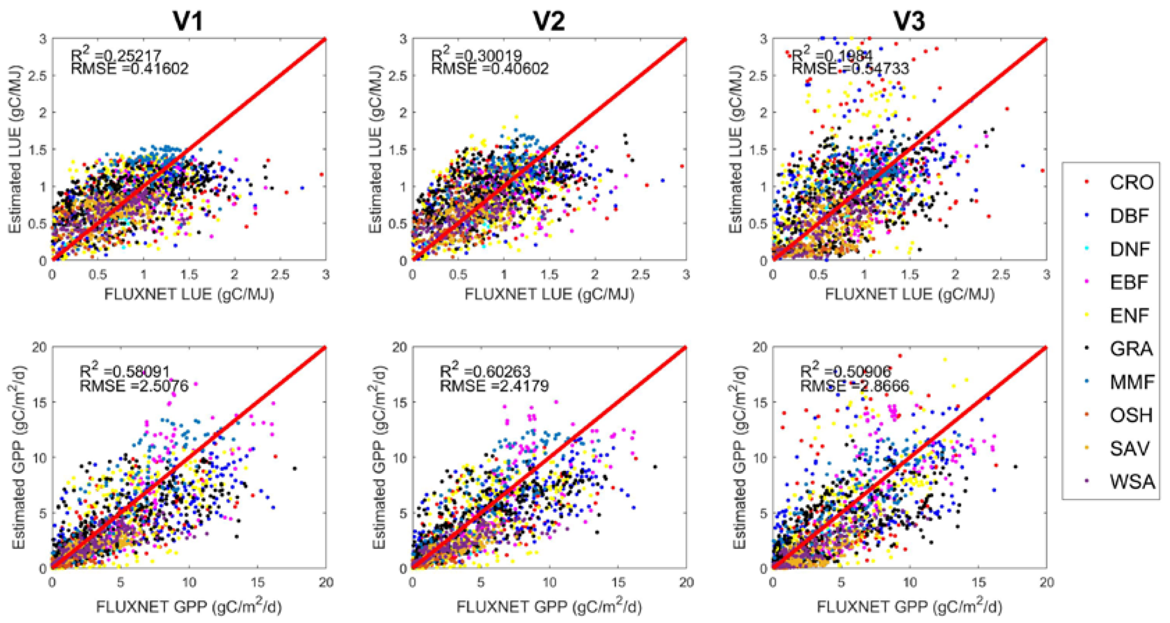
Figure 5.
The distributions of LUE by parameterization approach without the CI (V1).

Figure 6.
The distributions of LUE by the parameterization approach with the CI (V2).

Figure 7.
The distributions of LUE by the Cubist regression tree approach (V3).
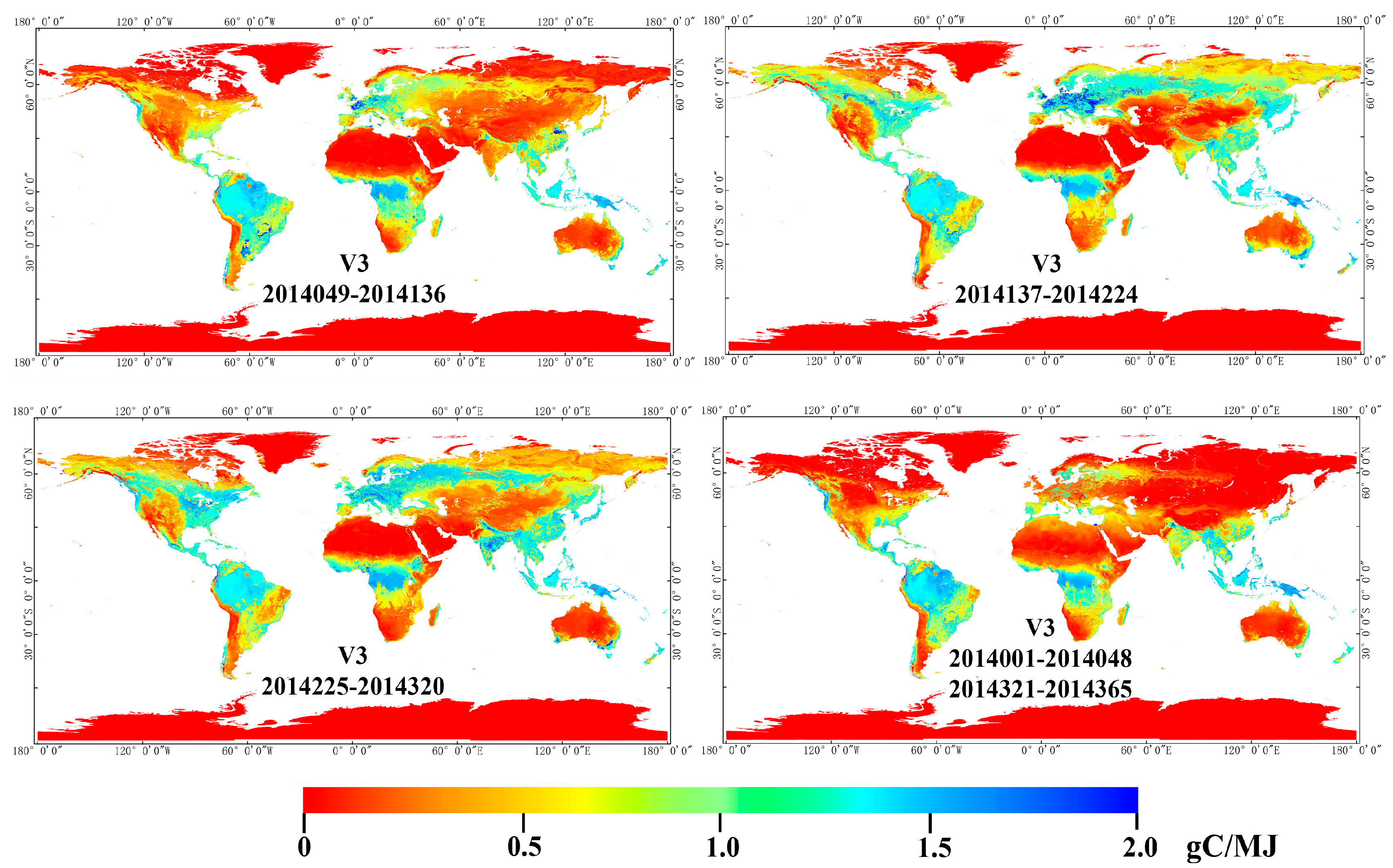
Figure 8.
The distribution of Annual GPP (gC/m2/yr) produced by parameterization approach without the CI (left upper), parameterization approach with the CI (right upper), Cubist regression tree approach (left middle), and MOD17 GPP in 2014 (right middle), the difference between V2 and MOD17 GPP (left lower), and the histogram of global annual GPP in 2014 by four algorithms (right lower).
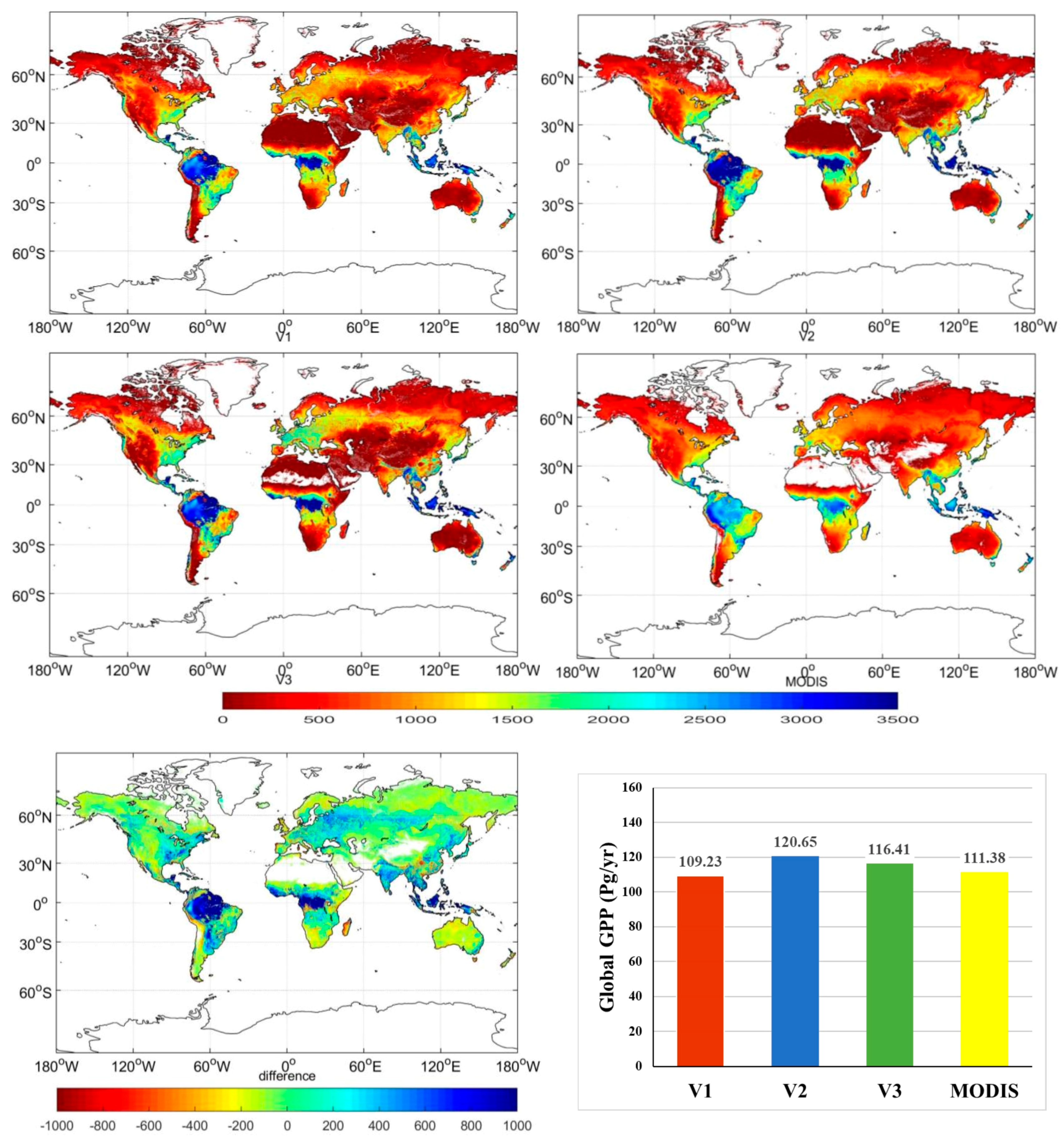
Figure 9.
LUE and GPP curves in IT-Isp, AU-Whr, CH-Cha and SE-St1.

Figure 10.
Global GPP in each type of vegetation. V1: Parameterization approach without the CI; V2: Parameterization approach with the CI; V3: Cubist regression tree approach.
Figure 10.
Global GPP in each type of vegetation. V1: Parameterization approach without the CI; V2: Parameterization approach with the CI; V3: Cubist regression tree approach.

Figure 11.
LUE and GPP curves along latitude. V1: Parameterization approach without the CI; V2: Parameterization approach with the CI; V3: Cubist regression tree approach.
Figure 11.
LUE and GPP curves along latitude. V1: Parameterization approach without the CI; V2: Parameterization approach with the CI; V3: Cubist regression tree approach.

Figure 12.
The curves of GPP (a), LUE (b), EF (c), PAR (d), Tmean (e) in CH-Lae (1) and US-SRG (2).

Figure 13.
Left: LUE and GPP curves and land surface images in homogeneous sites. US-WCr, US-Me2 and AU-Gin); right: LUE and GPP curves and land surface images in heterogeneous sites (DE-Kli and CH-Oe2) (red rectangles cover 500 m × 500 m land, yellow rectangles cover 5000 m × 5000 m land.
Figure 13.
Left: LUE and GPP curves and land surface images in homogeneous sites. US-WCr, US-Me2 and AU-Gin); right: LUE and GPP curves and land surface images in heterogeneous sites (DE-Kli and CH-Oe2) (red rectangles cover 500 m × 500 m land, yellow rectangles cover 5000 m × 5000 m land.

Figure 14.
LUE and GPP curves in US-Los and US-Tw4.


Table 1.
for each vegetation type.
| IGBP Vegetation Type | Vegetation Type Abbreviation | |||
|---|---|---|---|---|
| Evergreen Needleleaf Forests | ENF | 1.432 | 0.573 | 2.556 |
| Evergreen Broadleaf Forests | EBF | 1.491 | 0.596 | 2.603 |
| Deciduous Needleleaf Forests | DNF | 0.831 | 0.332 | 1.400 |
| Deciduous Broadleaf Forests | DBF | 1.434 | 0.573 | 2.556 |
| Mixed Forests | MF | 1.540 | 0.616 | 2.494 |
| Closed Shrublands | CSH | 1.168 | 0.467 | 2.070 |
| Open Shrublands | OSH | 0.761 | 0.304 | 1.510 |
| Woody Savannas | WSA | 1.120 | 0.460 | 2.298 |
| Savannas | SAV | 1.301 | 0.520 | 2.466 |
| Grasslands | GRA | 1.277 | 0.511 | 2.398 |
| Croplands | CRO | 1.587 | 0.943 | 2.466 |
Table 2.
Cubist regression tree approach.
| Rule 1 | conditions | vegetation type in {CRO, DNF, WSA, OSH, GRA}, LAI ≤ 0.7 and EF ≤ 0.753 |
| linear formula | LUE = 0.047 + 0.159 LAI + 0.78 EF − 0.11 CI | |
| Rule 2 | conditions | vegetation type in {DBF, SAV} and Tmean ≤ 11.562 |
| linear formula | LUE = -0.042 + 0.13 LAI + 0.62 EF + 0.0119 Tmean − 0.07 CI | |
| Rule 3 | conditions | vegetation type = WSA |
| linear formula | LUE = 0.338 + 1 EF - 0.006 Tmean + 0.02 LAI | |
| Rule 4 | conditions | vegetation type in {CRO, DNF, OSH, GRA}, LAI > 0.7 and EF ≤ 0.753 |
| linear formula | LUE = 0.207 + 1.08 EF + 0.091 LAI − 0.006 Tmean − 0.4 CI | |
| Rule 5 | conditions | vegetation type in {MF, ENF, EBF, CSH} and Tmean ≤ 11.562 |
| linear formula | LUE = 0.784 + 0.029 Tmean + 0.68 EF − 1.12 CI + 0.062 LAI | |
| Rule 6 | conditions | vegetation type in {DBF, SAV, MF, ENF, EBF, CSH}, Tmean > 11.562 and EF ≤ 0.753 |
| linear formula | LUE = 0.682 + 1.17 EF − 0.57 CI - 0.0066 Tmean + 0.014 LAI | |
| Rule 7 | conditions | LAI ≤ 1.8 and EF > 0.753 |
| linear formula | LUE = -0.514 + 0.409 LAI + 1.47 EF + 0.025 Tmean − 1.05 CI | |
| Rule 8 | conditions | vegetation type in {DBF, WSA, SAV, MF, GRA, ENF, EBF, CSH}, LAI > 1.8 and EF > 0.7531864 |
| linear formula | LUE = 0.862 + 1.26 EF − 1.41 CI + 0.021 LAI | |
| Rule 9 | conditions | CI <= 0.447, LAI > 1.8 and EF > 0.753 |
| linear formula | LUE = 0.439 + 1.71 EF − 0.93 CI | |
| Rule 10 | conditions | vegetation type = CRO, LAI > 1.8 and EF > 0.753 |
| linear formula | LUE = −0.831 + 3.24 EF + 0.0316 Tmean − 1.53 CI |
Table 3.
Light use efficiency (LUE) and gross primary productivity (GPP) validation for each type of vegetation.
Table 3.
Light use efficiency (LUE) and gross primary productivity (GPP) validation for each type of vegetation.
| IGBP | V1 | V2 | V3 | |||||||||
|---|---|---|---|---|---|---|---|---|---|---|---|---|
| LUE | GPP | LUE | GPP | LUE | GPP | |||||||
| R2 | RMSE (gC/MJ) | R2 | RMSE (gC/m2/d) | R2 | RMSE (gC/MJ) | R2 | RMSE (gC/m2/d) | R2 | RMSE (gC/MJ) | R2 | RMSE (gC/m2/d) | |
| CRO | 0.02 | 0.58 | 0.46 | 2.74 | 0.03 | 0.57 | 0.46 | 2.73 | 0.01 | 0.88 | 0.22 | 4.42 |
| DBF | 0.43 | 0.42 | 0.64 | 3.14 | 0.45 | 0.41 | 0.65 | 3.06 | 0.11 | 0.73 | 0.40 | 3.74 |
| DNF | 0.43 | 0.24 | 0.80 | 1.70 | 0.48 | 0.24 | 0.74 | 1.76 | 0.48 | 0.20 | 0.61 | 1.24 |
| EBF | 0.00 | 0.46 | 0.53 | 3.18 | 0.01 | 0.43 | 0.50 | 3.03 | 0.26 | 0.37 | 0.48 | 3.18 |
| ENF | 0.13 | 0.46 | 0.49 | 2.65 | 0.17 | 0.46 | 0.50 | 2.61 | 0.09 | 0.62 | 0.51 | 2.80 |
| GRA | 0.26 | 0.42 | 0.56 | 2.45 | 0.34 | 0.41 | 0.61 | 2.27 | 0.22 | 0.49 | 0.52 | 2.58 |
| MF | 0.29 | 0.37 | 0.72 | 2.29 | 0.36 | 0.35 | 0.72 | 2.15 | 0.20 | 0.37 | 0.64 | 2.16 |
| OSH | 0.10 | 0.31 | 0.21 | 0.88 | 0.19 | 0.28 | 0.31 | 0.86 | 0.07 | 0.35 | 0.23 | 1.13 |
| SAV | 0.06 | 0.26 | 0.48 | 1.52 | 0.19 | 0.23 | 0.54 | 1.51 | 0.12 | 0.35 | 0.32 | 2.01 |
| WSA | 0.38 | 0.29 | 0.62 | 1.82 | 0.38 | 0.29 | 0.66 | 1.81 | 0.55 | 0.26 | 0.70 | 1.73 |
1 Bold fonts represent the best result. V1: Parameterization approach without the CI; V2: Parameterization approach with the CI; V3: Cubist regression tree approach.
Table 4.
Detailed information for a few sites.
| Site ID | Site Name | Latitude (°) | Longitude (°) | Elevation (m) | Landcover | Mean Annual Temperature (°C) | Mean Annual Precipitation (mm) |
|---|---|---|---|---|---|---|---|
| IT-Isp | Ispra ABC-IS | 45.813 | 8.634 | 210 | DBF | 12.2 | 1300 |
| AU-Whr | Whroo | −36.673 | 145.029 | 152 | EBF | 16.7 | 625 |
| CH-Cha | Chamau | 47.210 | 8.410 | 393 | GRA | 9.5 | 1136 |
| SE-St1 | Stordalen grassland | 68.354 | 19.050 | 351 | WET | −0.7 | 303.3 |
| US-WCr | Willow Creek | 45.806 | −90.080 | 520 | DBF | 4.02 | 787 |
| US-Me2 | Metolius mature ponderosa pine | 44.452 | −121.557 | 1253 | ENF | 6.28 | 523 |
| AU-Gin | Gingin | −31.376 | 115.714 | 105 | WSA | 18.76 | 346 |
| DE-Kli | Klingenberg | 50.893 | 13.522 | 478 | CRO | 7.6 | 842 |
| CH-Oe2 | Oensingen crop | 47.286 | 7.734 | 452 | CRO | 9.8 | 1155 |
| US-Los | Lost Creek | 46.083 | −89.979 | 480 | WET | 4.08 | 828 |
| US-Tw4 | Twitchell East End Wetland | 38.103 | −121.641 | −5 | WET | 15.6 | 421 |
| CH-Lae | Laegern | 47.478 | 8.364 | 689 | MF | 8.3 | 1100 |
| US-SRG | Santa Rita Grassland | 31.789 | −110.828 | 1291 | GRA | 17 | 420 |
© 2020 by the authors. Licensee MDPI, Basel, Switzerland. This article is an open access article distributed under the terms and conditions of the Creative Commons Attribution (CC BY) license (http://creativecommons.org/licenses/by/4.0/).
Share and Cite
MDPI and ACS Style
Wang, M.; Sun, R.; Zhu, A.; Xiao, Z. Evaluation and Comparison of Light Use Efficiency and Gross Primary Productivity Using Three Different Approaches. Remote Sens. 2020, 12, 1003. https://0-doi-org.brum.beds.ac.uk/10.3390/rs12061003
AMA Style
Wang M, Sun R, Zhu A, Xiao Z. Evaluation and Comparison of Light Use Efficiency and Gross Primary Productivity Using Three Different Approaches. Remote Sensing. 2020; 12(6):1003. https://0-doi-org.brum.beds.ac.uk/10.3390/rs12061003
Chicago/Turabian StyleWang, Mengjia, Rui Sun, Anran Zhu, and Zhiqiang Xiao. 2020. "Evaluation and Comparison of Light Use Efficiency and Gross Primary Productivity Using Three Different Approaches" Remote Sensing 12, no. 6: 1003. https://0-doi-org.brum.beds.ac.uk/10.3390/rs12061003
Note that from the first issue of 2016, this journal uses article numbers instead of page numbers. See further details here.