The Polarimetric Sensitivity of SMAP-Reflectometry Signals to Crop Growth in the U.S. Corn Belt


1
Planetary Radar Radio Science Systems Group, Jet Propulsion Laboratory, California Institute of Technology, Pasadena, CA 91109, USA
2
Microwave Instrument Science Group, Jet Propulsion Laboratory, California Institute of Technology, Pasadena, CA 91109, USA
*
Author to whom correspondence should be addressed.
Remote Sens. 2020, 12(6), 1007; https://0-doi-org.brum.beds.ac.uk/10.3390/rs12061007
Submission received: 20 February 2020
/
Revised: 18 March 2020
/
Accepted: 19 March 2020
/
Published: 21 March 2020
(This article belongs to the Special Issue Applications of GNSS Reflectometry for Earth Observation)
Abstract
:Crop growth is an important parameter to monitor in order to obtain accurate remotely sensed estimates of soil moisture, as well as assessments of crop health, productivity, and quality commonly used in the agricultural industry. The Soil Moisture Active Passive (SMAP) mission has been collecting Global Positioning System (GPS) signals as they reflect off the Earth’s surface since August 2015. The L-band dual-polarization reflection measurements enable studies of the evolution of geophysical parameters during seasonal transitions. In this paper, we examine the sensitivity of SMAP-reflectometry signals to agricultural crop growth related characteristics: crop type, vegetation water content (VWC), crop height, and vegetation opacity (VOP). The study presented here focuses on the United States “Corn Belt,” where an extensive area is planted every year with mostly corn, soybean, and wheat. We explore the potential to generate regularly an alternate source of crop growth information independent of the data currently used in the soil moisture (SM) products developed with the SMAP mission. Our analysis explores the variability of the polarimetric ratio (PR), computed from the peak signals at V- and H-polarization, during the United States Corn Belt crop growing season in 2017. The approach facilitates the understanding of the evolution of the observed surfaces from bare soil to peak growth and the maturation of the crops until harvesting. We investigate the impact of SM on PR for low roughness scenes with low variability and considering each crop type independently. We analyze the sensitivity of PR to the selected crop height, VWC, VOP, and Normalized Differential Vegetation Index (NDVI) reference datasets. Finally, we discuss a possible path towards a retrieval algorithm based on Global Navigation Satellite System-Reflectometry (GNSS-R) measurements that could be used in combination with passive SMAP soil moisture algorithms to correct simultaneously for the VWC and SM effects on the electromagnetic signals.
Keywords:
GNSS-R; SMAP-R; VWC; vegetation opacity; crop type; crop height; soil moisture; crop health; crop productivity; agriculture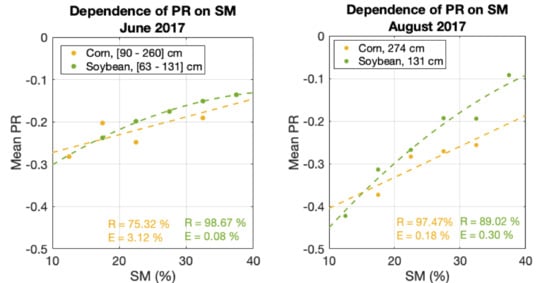
1. Introduction
Sustaining and enhancing the economical production of crops continues to be an important focus of agricultural research. Information and knowledge on crop vegetative growth and crop reproductive development is vital to agricultural producers with the goal of more efficient production of high-quality crops. Vegetative growth of crops is defined as the accumulation of dry matter, which is the weight of the crops including all its constituents, excluding water. For example, the vegetative stage of corn begins when the seedling emerges and continues until tasseling, when the reproductive stage begins. During the vegetative stage, leaves develop and grow, the stalk forms, and reproductive structures (ear and tassel) begin to form. The reproductive development of crops is related to the crop transition into the reproductive phase. Reproductive development stages begin with fertilization of the floret (pollination) and end when the grain reaches its maximum dry weight. This later stage is called physiological maturity. To ensure high productivity of the crops, there are certain requirements that need to be met at the crop growth and development stages. By understanding how corn grows and develops, producers can more confidently assess crop damage, estimate if it will recover, and apply herbicides and other crop treatments at the best time. Information on soil conditions and crop growth related parameters, such as the vegetation water content (VWC) at every stage, are the main factors that can help understand the final crop’s production.
Missions like the Soil Moisture Active Passive (SMAP) [1] and the Soil Moisture Ocean Salinity (SMOS) [2] are currently providing information on the soil moisture (SM) conditions at scales of 9 km × 9 km [3] in the case of SMAP and 25 km × 25 km [4] in the case of SMOS. Note that for the SMAP product, event it is posted to the 9km × 9km grid, and the representative area of each grid cell is 36 km. In [5], it was found that the performance of the enhanced 9 km SMAP SM product was equivalent to that of the standard 33 km SMAP SM product, attaining a retrieval uncertainty below 0.040 m3/m3 unbiased root-mean-squared error and a correlation coefficient above 0.800. Soil moisture estimation remains a challenge due to the lack of validated VWC products at a global scale at a temporal resolution that matches the speed of the crop growth. VWC impacts the electromagnetic signals through volume scattering due to the leaves, branches, trunks, and attenuation due to the dielectric constant of the vegetation. The transmissivity, computed as , describes the amount of soil emission passing through the vegetation layer. The transmissivity depends on both the incidence angle and the vegetation opacity (VOP), computed as , where is a parameter describing the vegetation type [6]. Note that VOP and vegetation optical depth (VOD) are synonymous. Therefore, VWC impacts the microwave emission received by SMAP such that under the same soil moisture conditions, differences in VWC result in different microwave emissions from the same surface. In trying to estimate soil moisture, the lack of VWC information results in an uncertainty of the soil moisture retrievals. The availability of high spatial and temporal resolution global estimates of VWC would therefore improve SM estimates. In particular, the SMAP mission has developed a VWC dataset used in generating SMAP science data products, based on Moderate Resolution Imaging Spectroradiometer (MODIS) [7] data. The drawback of the MODIS-based product is that it relies on Normalized Differential Vegetation Index (NDVI) as a proxy to VWC; NDVI loses sensitivity to VWC as the water content increases [8]. In addition, the SMAP VWC products are based on 10-day NDVI climatology of 10 years (2000 to 2010), and this results in SM errors when vegetated areas undergo dynamic changes, as is sometimes the case within agricultural landscapes. Other approaches include large-scale mapping of VWC [9], but the validity is limited by the data used. Even so, VWC datasets are not updated routinely. For agricultural areas characterized by very dynamic landscapes in terms of SM, VWC, VOP, and vegetation height, a 10-day independent VWC product would have a great impact on the soil moisture retrievals obtained by satellite missions as SMAP. Limited in situ measurements are obtained, but those are usually sparse and cover only limited crop types. In order to understand the impact of using products based on climatology, it is important to understand first the dynamics of the vegetated landscapes: forest of any type, tundra, meadows, and in general, the majority of natural spaces not used for the purpose of agriculture are less dynamic vegetated landscapes, and therefore, their VWC signature changes less drastically in a seasonal regime. For most natural spaces, the low-frequency nature of their VWC variations produces a high correlation between VWC seasonal climatology and real-time VWC [10]. Equally, when considering VOP (dependent on VWC) information, agricultural areas will show a bigger discrepancy between seasonal climatology and daily estimates as compared to natural spaces. Another descriptor of the vegetation is the vegetation height, i.e., the thickness of the vegetation layer. The vegetation height for agricultural landscapes is very dynamic during the growing season and may change in scales of a few days. Therefore, some vegetated landscapes are well represented with a static/seasonal information, while agricultural areas need finer temporal scales.
In August 2015, the SMAP mission started collecting GPS signals as they scatter off the Earth’s surface [11,12,13,14,15]. These signals are measured by the SMAP radar receiver, whose band pass filter center frequency was switched to the GPS L2C band (1227.6 MHz). These bistatic radar L-band signals are measured at V-polarization and H-polarization simultaneously. Since bistatic radar and radiometer measurements are impacted by vegetation cover differently [16,17], the combination of both active (SMAP-R) and passive (SMAP radiometer) measurements could act to further constrain vegetation effects for the SM retrieval. SMAP-R based vegetation parameters are independent of any NDVI product and could improve SM estimation performance. There have been previous studies employing left hand and right hand circularly polarized GNSS-R measurements to compute a polarimetric ratio, such as [18,19] and a previous work using SMAP-R data [12].
This manuscript presents a sensitivity analysis of the SMAP-R signals to VWC, VOP, crop height, and type, including corn and soybean. The impact of SM on the sensitivity to the crop growth parameters is also assessed. The analysis is limited to an area characterized by low roughness: the United States Corn Belt during the 2017 crop season. Section 2 describes the SMAP-R measurements and presents the main observable used in this study, the polarimetric ratio (PR), as well as provides a discussion on the spatial resolution of SMAP-R measurements. Section 3 explains the methodology and analyzes each one of the datasets involved in the process. In Section 4, we investigate the variability of the PR through the crop season and the sensitivity of the PR to crop growth parameters. Section 5 discusses a path towards a retrieval algorithm based on Global Navigation Satellite System-Reflectometry (GNSS-R) and on improvements and requirements for future research. Section 6 states the final conclusions of this study.
2. SMAP-R Measurements Description
The GPS signals reflected off the Earth’s surface are collected at the SMAP radar receiver in the form of in-phase and quadrature (I/Q) samples. The I/Q samples are publicly available at the NASA Earthdata website [20]. Using a modified version of the SMAP-R processor used in [11,12], data are filtered for those geometries where there is potential to capture a specular point, i.e., within the -3 dB beam width of the SMAP antenna pointed to 40°, which provides a range of incidence angles between 37.3° and 42.7°. This selection ensures that the measured specular points are not degraded by the decay of SMAP antenna gain away from −3dB. Those selected I/Q samples are post-processed into delay-Doppler maps (DDM) [21,22], with a 5 ms coherent time and 25 ms incoherent time (five incoherent accumulation). A DDM is defined as the delay and Doppler power distribution of the GPS signal scattered over the Earth’s surface. Since the SMAP antenna rotates, consecutive DDMs integrated at 25 ms are spaced approximately 25 km apart. The DDMs are then calibrated to account for GPS transmitter power and GPS antenna gain at the reflection angle and also for the filtering effect of the SMAP high gain antenna, whose small footprint partially observes the scattering surface. The next subsection provides more details on the calibration performed to the DDM and the observables used in the assessment of VWC estimates.
2.1. SMAP-R Calibration
To calibrate the SMAP-R DDMs, we applied the modified equation presented in [15]. The equation in [12] followed the CYclone Global Navigation Satellite System (CYGNSS) [23,24,25] mission calibration procedure presented in [26], but adds the filtering effect of the SMAP antenna pattern. The equation takes the form in eqn. (1):
where:
- is the DDM received power distribution at each delay and Doppler bin.
- is the coherent integration time. = 25 ms for SMAP-R data, instead of the typical value of 1000 ms used in other GNSS-R missions.
- is the GPS transmitted power.
- is the GPS transmitter antenna gain.
- is the GPS signal wavelength (at GPS-L2C is 24.42 cm).
- corresponds to the distance from the transmitter specular point.
- corresponds to the distance from the receiver to the specular point.
- is the SMAP antenna gain value at the specular point incidence angle . It is computed from eqn. (2), where we assume the gain presents a linear decay within the −3 dB beam width (2.7 deg.) that goes from its maximum value ( = 36 dBi @ 40 deg. incidence angle pointing) to 33 dB.
- is the filtered effective surface scattering area. It is computed following the methodology described in [15], where the size of the area corresponding to each and bin filtered by the SMAP antenna is normalized to the size of the same and bin considering an omnidirectional antenna.
The calibration methodology developed in [15] and implemented in this study considers two corrections:
- Calibration of the direct power information (). is calibrated by collocating CYGNSS information for the same day of measurements.
- Calibration of the SMAP antenna filtering effect ().
SMAP-R measurements have a non-uniform spatial resolution. The variability on the spatial resolution is linked to the nature of the SMAP-R signals, since the spatial resolution depends on the characteristics of the scattering area. A rougher surface enlarges the scattering area, enlarging the spatial resolution. The presence of vegetation also enlarges the spatial resolution as equally, it results in the scattering coming from a more extensive area. To compute the approximate spatial resolution of each measurement, we applied the methodology also explained in [15]. According to the results in [15], a threshold of 70% was selected, and the delay gathering the 70% of the power was transformed to an ellipse of constant delay on the surface (iso-delay line) [21]. The size of the scattering area was set to the semi-major axis of the computed ellipse to represent the scattering area of that particular measurement. Figure 1 shows the variability on the scattering area sizes computed for two extreme scenarios: (1) bare soil, characterized by low VWC, low height, and low VOP; and (2) crop seasonal growth peak, characterized by high VWC, high height, and high VOP. The two extreme scenarios were selected as the reference states (RS1 and RS2, respectively) of our dataset and will be further explained in Section 3.
The spatial resolutions observed in the measurements involved in this study were between 5 km and 24 km, depending on the crop type and growth stage that characterize the scattering surface. The mean of the bare soil conditions was ~12 km, while for the same area, after crop grew, the observed spatial resolution increased to a mean of ~17 km. Our conclusions agreed with the results presented in [15], where an expected spatial resolution between 5 km to 26 km was acceptable for none to high vegetation, although roughness conditions and the surface topography had an impact on the final spatial resolution. For the purpose of this study, analyzing the sensitivity, and in order to easily match the spatial resolution of the reference products used in this study (SMAP SM and VWC), we used a simplistic strategy of gridding the SMAP-R data to a 9 × 9 km where all specular points falling within each grid cell were considered to contribute only to that grid cell and were averaged together. Future research focused on generating products from this dataset will include the appropriate spatial resolution gridding.
2.2. The Observable: Polarimetric Ratio
We used an observable built from the DDM power information, in particular the power of the peak. Due to the complexity of the filtering effect of the SMAP antenna, we decided not to include any observable based on the shape of the DDMs. Therefore, the corrections described in Section 2.1 were only applied to the and bin that corresponded to the peak of the DDM. The observable used in this study was the polarimetric ratio (PR). PR was computed as in [27] using the formula:
where:
- is the delay at the bin of the DDM peak.
- is the frequency Doppler at the bin of the DDM peak.
- is the DDM received power at H-polarization measured by SMAP-R at .
- is the DDM received power at V-polarization measured by SMAP-R at
The sensitivity of SMAP-R signals to crop growth will therefore be evaluated through the variability of the PR observable to changes on crop growth parameters (VWC, VOP, NDVI, and crop height), as well as SM conditions.
3. Methodology
In order to analyze the sensitivity of SMAP-R signals to the crop growth parameters, we selected data collected from the United States (U.S.) Corn Belt, an extensive agricultural area that is planted with primarily corn, soybean, and wheat every year. Figure 2 shows information on the U.S. Corn Belt.
Figure 2a shows the selected site with information from the U.S. Department of Agriculture (USDA) National Agricultural Statistics Service (NASS) database [28] showing the amount of planted corn acres per county. The number of acres planted varies year-to-year as can be seen in Figure 2b. SMAP-R data allowed for the temporal series analysis of the U.S. Corn Belt seasonal changes from 2016 to 2019. The maps shown are available at [28]. Figure 2c shows a sketch of the growth stages of a corn plant. Figure 2d to Figure 2f show images of different stages of the corn, bare soil, plant growing, and harvesting, respectively.
The sensitivity analysis of SMAP-R measurements was therefore explored over the U.S. Corn Belt. We used the observable, PR, described in Section 2.2. The methodology implemented is illustrated in Figure 3.
Summarizing Figure 3, there are three main steps:
- SMAP-R data preparation: computing PR and gridding the data.
- Use of ancillary datasets: gathering information on roughness, SM, and crop type using it to filter and bin the PR observable.
- Sensitivity analysis: Analyze PR observable against reference datasets; i.e., VWC, VOP, NDVI, and crop height.
The next subsections provide detailed information on the key elements shown in Figure 3: the two-state analysis strategy, the ancillary datasets employed to characterize the scattering area and the resulting grouped the data, as well as the reference datasets used to explore the sensitivity of the SMAP-R signals to the crop growth parameters (VWC, VOP, NDVI, crop height). Sensitivity analysis are provided in Section 4.
3.1. Two-State Analysis Strategy
SMAP-R measurements have low sampling and poor coverage, but those characteristics can be overcome by implementing analysis strategies as using measurements over long periods of stability in two extremes as the references and analyzing the variability of the measurements in transitional periods. We refer to this as a two-state analysis strategy. We analyzed the mean variability of the observable PR, described in Section 2.2, at these two states. Data between states could then be analyzed at shorter times referencing them to the two extreme states and discarding samples that are out of the limits marked by the two reference states.
In this study, we averaged the information from two months, March and April 2017, as one reference state describing the bare soil conditions (no VWC, 0 VOP, 0 cm crop height: reference state RS1). We used July and August 2017 as the other reference state describing the season peak of the crops (high VWC, high VOP, high height: reference state RS2). The transitional periods from especially April to July 2017 (growing period with increasing VWC, VOP, and height) and August to October 2017 (drying period with decreasing VWC, low height variability, and harvesting) would therefore be referenced to the two reference states described. Data that did not fall within the PR ranges identified for the reference states RS1 and RS2 were discarded. Figure 4 shows the PR observable for the two reference states.
PR plots were computed using a fixed grid of 9 × 9 km to match current official SMAP products. Both and were then computed and used to derive the PR values, as described in eqn. (1). Note that PR values, computed from the forward scattered GPS signal after it interacted with the vegetation, differed from those expected in the radiometry field. PR values were averaged together using a drop in the box approach, i.e., measurements whose specular points fell within each grid cell were averaged together (regardless of their true spatial resolution). Figure 4 shows the heterogeneity of the PR observable; i.e., it shows the variability within the scene due to differences in the crop type and growth stage during the selected period, as well as the variability of the soil moisture conditions. For bare soil and constant roughness conditions (Figure 4a), the variability was due primarily to soil moisture. During the peak season (Figure 4b), VWC, VOP, crop height, crop type, and soil moisture played an important role. From Figure 4, a general drop in the levels of the PR observable can be observed. In Section 4, we provide a deeper analysis of the SMAP-R signal sensitivity to the different geophysical parameters that compose the scene.
3.2. Ancillary Datasets
Below, we describe the ancillary information used to filter and bin our data as a part of the process outlined in Figure 3: crop type, surface roughness, and monthly soil moisture variability.
The USDA NASS CropScape–Cropland Data [30] provides information on the type and quantity of crops per county in the U.S. and is freely available at [30]. We used the information in the dataset to assign the predominant crop type to a pixel of 9 km × 9 km, matching SMAP spatial resolution, for the year 2017. The map is shown in Figure 5.
Following the methodology described in Figure 3, the crop type information was used to analyze the SMAP-R PR observable for the different crops separately avoiding the mix due to the different scattering properties characteristic of each crop type and distinguishing effects of the different growth stages of each crop type.
Roughness had a big impact on the variability of the strength of the SMAP-R signals, as well as the variability of the spatial resolution of the measurements. The United States Corn Belt crop area presented a low surface roughness with small variability. SMAP’s roughness ancillary product [31,32], stored in the SMAP SM official product, corroborated this statement (see Figure 6).
The SMAP roughness ancillary dataset is a static product. Even where the roughness as low (orange areas) as compared to surrounding rougher (red) areas, the assumption that the roughness was static was imperfect. We recognized that roughness varied throughout the year in the U.S. Corn Belt, primarily due to tillage [33]. Tillage may occur after harvesting the previous season and before the first snowfall—around November—or after the snow melts in spring—around March. In addition, this tillage was spatially variable, as it depended on farm management practices. Additionally, rainfall smooths the soil surface [33] until the crops grow and can shelter the surface. Therefore, both the tillage and the rain smoothing affect the roughness of the area dynamically rather than statically—as was assumed in this work. This assumption was one source of error in our analysis of the relationships between observations and geophysical parameters explored in this study: SM, VWC, VOP, and vegetation height. Given limited information on tilling and other dynamic variables, we utilized the static product stored in the official SMAP SM product and acknowledged that this may limit the robustness of the analysis herein.
Much of the central region shown in Figure 6 had a roughness value of around ~0.1 with little variability in the surrounding agricultural areas. The roughness ancillary product is a static product that has been modeled as the surface reflectivity of a rough surface () computed as the surface reflectivity of a smooth surface () multiplied by a factor dependent on a parameter () linearly dependent on the root-mean-squared surface height [34,35] and the incidence angle () as: , with ; see [36]. Fresnel equations were used to compute at each polarization; see [36]. For SMAP, values were obtained from a land cover-driven lookup table, available in [37]. The roughness values corresponded to unitless values that were indicative of bare soil roughness within SMAP 9 km grid cell (0 min, 1 max). For this study, we selected those areas in the map that had a low roughness with low variability (orange area in Figure 6). Using the roughness information, we generated a mask where roughness value remained between the range [0.1–0.112], shown in Figure 7a, and we used this map to filter the crop information (Figure 7b).
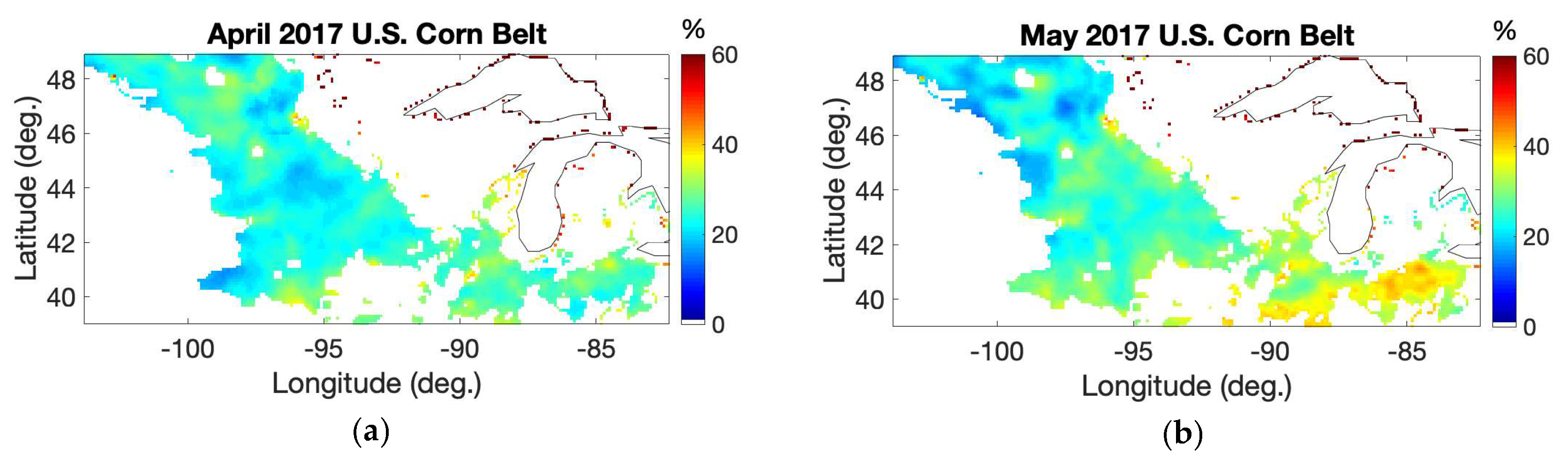
After using the roughness mask, there were only three types of crop to include potentially in our study: great extensions of corn and soybean and some areas in the northern part of wheat. The next important parameter to control in the area under study was the SM, whose variability would have an impact on the reflected signal strength, and therefore on the PR. To isolate the impact of SM on the sensitivity to crop growth parameters, we used the SMAP SM official product at 9 × 9 km [3]. Figure 8 shows the mean and standard deviation of the SM on a monthly basis for areas represented by each crop type. In addition, in Appendix A, we included the monthly averaged SMAP SM maps from April 2017 to November 2017. SM values are expressed in units of % throughout the manuscript. The % corresponds to the volumetric soil water content computed from the volume of water (cm3) over the volume of soil (cm3) expressed in percentage.
The monthly means of SM observed by the SMAP mission in our area under study showed high variability. During May and June, SMAP soil moisture retrievals showed an increase in soil moisture, most probably due to rain events since most part of the area under study was rain-fed. Rain benefits the growth and health of the crops. During the months of July, August, and September, SM variations seemed to decrease linearly in the mean. During October, variations in soil moisture were also observed for most of the fields and were also probably due to rain events. We used these data in order to understand what the impact of SM variation on the sensitivity of SMAP-R signals to the crop growth parameters was. In order to do this and following the scheme presented in Figure 3, we initially binned together areas with SM values in the range of 0% to 40% in steps of 5%, providing a total of eight levels of SM, and then analyzed the sampling population of binned PR values to discard those statistically poorly represented. We defined those statistically poorly represented SM ranges with a number of samples below five for most of the PR bins. This analysis is presented in Section 4.
3.3. Reference Datasets
Following the scheme in Figure 3, in order to study the sensitivity of SMAP-R signals to the different crop growth parameters, we selected a number of reference datasets: the VWC from the SMAP ancillary dataset, the VOP from the SMAP ancillary dataset, and the crop height that was estimated from information on typical growth values for the different crop types.
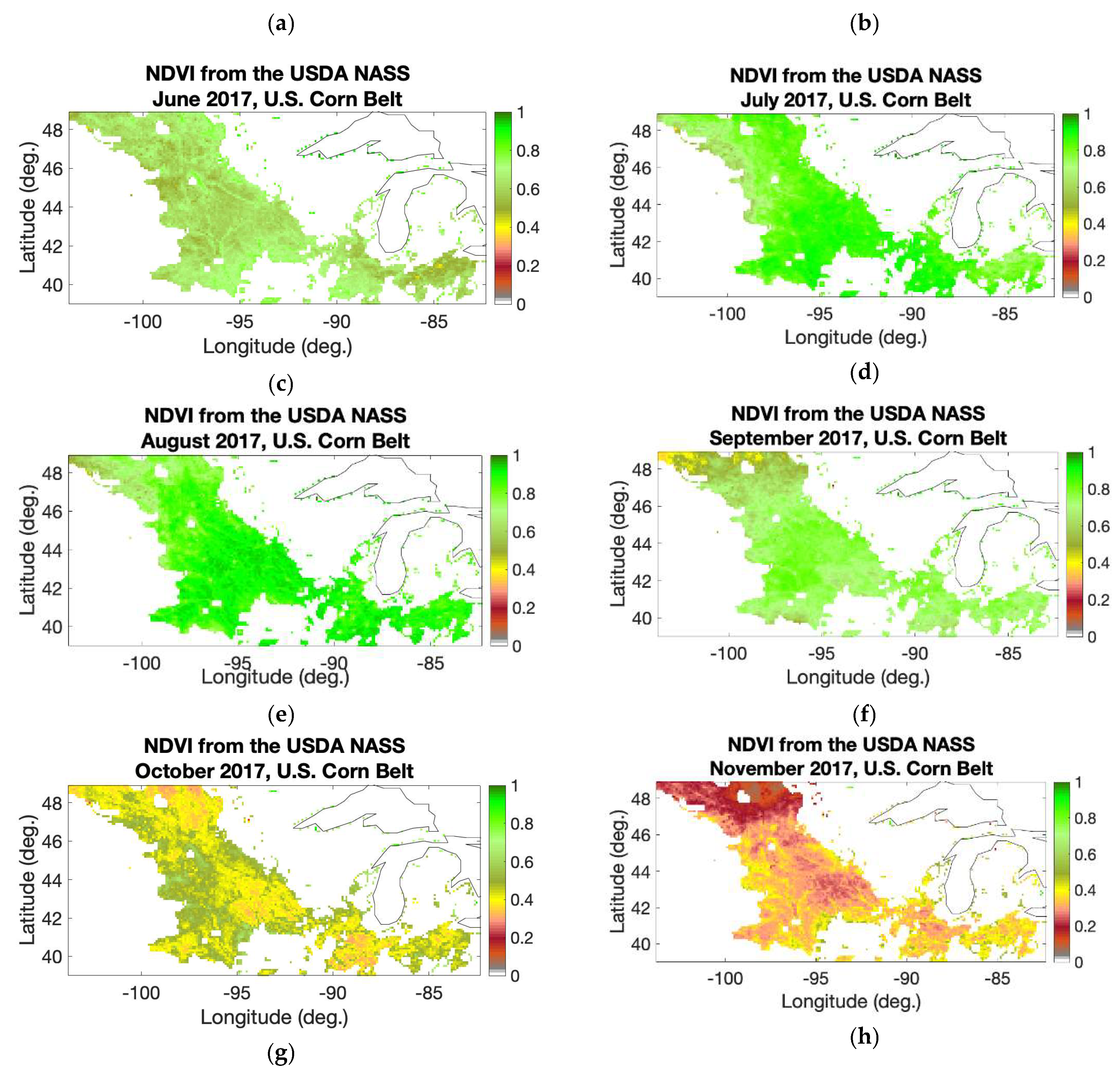
The NDVI reference dataset was obtained from the NDVI product from the USDA NASS VegScape–Vegetation Condition Explorer [38], where MODIS measurements were employed to derive the NDVI measurements. Appendix A shows the NDVI maps for the whole crop season (April to November, 2017). Figure 9 shows the mean and standard deviation of the NDVI on a monthly basis for areas represented by each crop type.
The NDVI provides a numerical indicator used to assess whether the observed surface contains live green vegetation or not. As can be seen in Figure 9, NDVI showed the highest values during July and August 2019 for both corn and soybean crop types. In the case of wheat, the peak of the season happened in June.
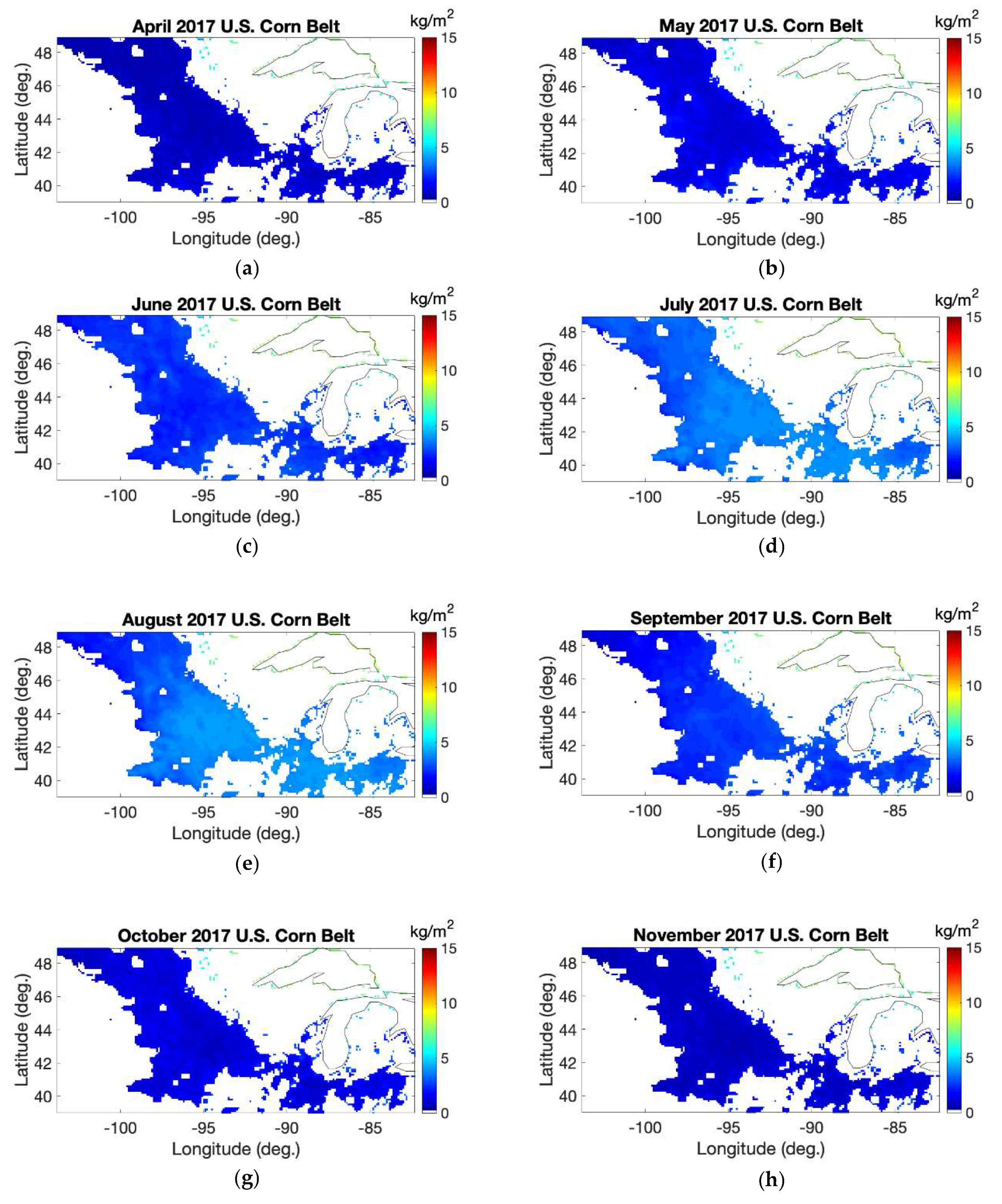
The selected VWC and VOP reference datasets were those stored as ancillary products in the SMAP SM official product [3]. VWC and VOP products used in this study were therefore derived from 10 day NDVI climatology rather than obtained from actual 2017 data. We included monthly averaged VWC and VOP maps in Appendix A. Because VWC and VOP were derived from NDVI climatology, there would be a correlation between all three products; even the selected NDVI reference was derived from actual measurements. Some differences were expected because VWC estimations considered foliage and stem components adjusted for land cover types using the MODIS International Geosphere Biosphere Programme (IGBP) classification scheme [39], and therefore, the analysis of the VWC could add information that the NDVI dataset was missing. Equally, since VOP was computed from VWC estimations, the two products would be correlated and would provide similar information. Because VOP was computed as the VWC multiplied by a b-factor and this b-factor was dependent on the type of vegetation and the measurement frequency, the VOP dataset may bring relevant information that both NDVI and VWC were missing. Figure 10a,b respectively show the mean and standard deviation of the VWC and VOP datasets in a monthly basis for areas represented by crop type.
As can be seen from Figure 10 and as expected, both VWC and VOP were very similar products that showed a high dependency on NDVI (Figure 9). It is important to note that a comparison against VWC and VOP based on real measurements, rather than climatology, would have been more accurate. By using a climatological dataset, we would observe larger errors due to the real variability of the fields not captured by the selected reference datasets. In [40], the authors compared SMAP VOP (based on climatology) and SMOS VOP (based on real data) in the South Fork Network in Iowa day-to-day for three seasons (in 2015, 2016, and 2017), and the general trends of both products were very similar. This work intends to demonstrate that SMAP-R contains information related to crops and does not support a geophysical model function derived from the selected VOP dataset. The average month-to-month VOP changes were well represented by the selected reference VOP and therefore could be used to determine SMAP-R sensitivity to crop growth. In the next sections, we will analyze the dependence of SMAP-R signals on NDVI, VWC, and VOP.
Each crop had a different associated growth rate. The crop height was therefore a function of the crop type, which was represented by a particular growth speed and final height. In order to understand if the thickness of the vegetation layer affected the SMAP-R signals, it was important to add the crop height to our analysis. We were not able to find a monthly product of the vegetation height over the U.S. Corn Belt during 2017, and for this reason, we developed an algorithm to estimate the crop height evolution. The generated product may not be accurate at a daily rate, but it proved sufficient information for monthly mean analysis. Characterizing agricultural fields is a difficult task since there is a lack of seasonal ground-truth, such as yearly updated information on the specific variety of crops of each field or the planting date. In addition, there are also many aspects that can be different not only year-to-year, but also field-to-field, and even plant-to-plant. We made assumptions on the height of the plants based on a few field studies, but we recognized these assumptions may not always be robust. The algorithm was mainly based on standard knowledge for the growth stages of a specific crop type and the initial time at which the crops started to grow. The initial growth time was obtained from the NDVI dataset. For the crop growth (height vs. days from emergence), we employed information available from previous studies and various resources ([41,42,43]). The values provided from those studies were used as the representative means of the fields for each crop type. Although not accurate to specific plants, the overall growth was expected to be robust enough for testing the monthly sensitivity of SMAP-R to crop height. Since there were only three types of crops within our study area, we limited the information to corn, soybean, and wheat. The information is shown in Table 1, Table 2 and Table 3.
The methodology used to generate crop height information is shown in Figure 11.
The information in Table 1 to Table 3 was used in combination with crop type information in Figure 7b to identify which area of the surface corresponded to each crop type. Using NDVI change information at a weekly rate, we determined the first phase of vegetation presence for each 9 × 9 km pixel and assigned an estimated initial growth day. Following the methodology in Figure 11, we used the 9 × 9 km grid initial day map, the crop type information, and the information in Table 1 to Table 3 to create the crop height maps showing the estimated mean height of the plants at a monthly rate. Those are included in Appendix B. Figure 12 shows the mean and standard deviation of the crop height on a monthly basis for areas represented by each crop type.
The resulting crop mean height information represents an estimated height of the predominant crops within each grid cell every month, from April to November 2017. Corn presented in general a higher standard deviation. The higher standard deviation occurred in June and could be explained through the height variability of corn plants growing from 50 cm to 250 cm in a matter of two months. This period of high variability was directly linked to the initial day of growth at the pixel level found through NDVI measurements using the methodology in Figure 11. Differences in the start day would cause differences in growth, and because the plants grew ~150 cm in a short period of time, this translated into dispersion. As mentioned at the beginning of this subsection, the validation of the height maps was not feasible since we were not able to find ground-truth data for the U.S. Corn Belt during the 2017 growing season. Nevertheless, since we were doing monthly averages of the typical crop height values at 9 km × 9 km, we believe the approach was accurate for our purposes and that the crop growth observed for all plants was reasonable. We wanted to observe if there was an overall correlation between monthly averages of crop height and monthly averages of peak SNR; even though there was a bias on the crop height or an incorrect final height assumption, correlation should still show the sensitivity of SMAP-R signals to crop height. Since there was no validation of the height maps, absolute relationships between the two variables would not be possible.
4. Sensitivity Analysis
This section shows the results obtained following the methodology outlined in Figure 3. A sensitivity analysis was performed using the SMAP-R gridded data, the roughness information, soil moisture information, crop type information, and the reference datasets VWC, VOP, NDVI, and crop height, following Steps 1, 2, and 3, as described in Figure 3. As a first step, we applied the roughness mask (Figure 7b) to the PR observable, and we binned the data using the soil moisture information for each crop type. Therefore, the resulting roughness-filtered data were binned into eight SM ranges, from 0 to 40% in steps of 5%, and separated into different crops: corn, soybean, and wheat (the only crop types present within our roughness mask). After grouping the data, we selected SM ranges with enough samples to be statistically representative. We then analyzed the monthly variations of the different observables and correlated those variations to crop growth parameters: VWC, VOP, NDVI, and crop height.
4.1. PR Sample Distribution
First, the PR sample distribution for five different SM ranges and for each crop type is shown in Figure 13.
As was shown in Figure 5, there was only a small area of wheat on the north-east part of the area under study. Figure 13 proves that the crop type wheat was not well represented for any of the SM ranges. We excluded wheat when analyzing the data, which stayed below five samples for all PR bins and all SM ranges. Corn and soybean had a good representation of samples for SM ranges [15–20]%, [20–25]%, and [25–30]%. Ranges [10–15]% and [30–35]% showed a reduced number of samples, and the results would show a higher uncertainty over those ranges. There were no samples below SM = 10% or over SM = 35%. Consequently, we performed the sensitivity analysis of the SMAP-R PR observable to corn and soybean crop types within the SM ranges [10–15]%, [15–20]%, [20–25]%, [25–30]%, and [30–35]%.
4.2. Variability of the PR during the Crop Season
In order to analyze the PR observable on a month-to-month basis, we performed a pre-calculation of the minimum and maximum values expected for bare soil (reference state RS1) and high peak season conditions (reference state RS2), using a two-month average. We observed the PR mean transitioning from RS1 state to RS2 state and the as it dries and gets harvested transitions back to RS1 state. We then analyzed the monthly mean and standard deviation of the PR observable through the season, discarding values that were showed to be outliers based on RS1 and RS2 (~3% of the data). Figure 14 shows the temporal analysis of PR, for two of the SM ranges.
Figure 14 shows that PR showed a clear signature that decreased as crops grew and returned to initial levels after harvesting (October-November). For each plot in Figure 14, SM variation was less than or equal to 5%, roughness variation was minimal, and crop type is shown with different colors. Note that the two selected SM ranges showed similar seasonal behavior, but the PR dynamic range of the higher SM range was reduced. Figure 14a shows a PR drop for corn crop type. This drop could be explained by the dynamic roughness effects since corn is usually tilled post-harvest, causing an increase in roughness. Soybean is occasionally left on the surface with no tilling. An increase in the surface roughness, especially after harvesting, could impact the PR together with SM variations. To investigate this effect, Figure 15 shows the dependence of PR on SM. We selected April and November as representative of bare soil condition and harvested fields, respectively, and June and August as representative of growing season with two levels of growth, intermediate and peak.
Under bare soil conditions, as April and November plots, the relationship between the polarimetric ratio and the soil moisture showed a linear behavior. For the November plot (Figure 15d), the surface was not actually bare soil as it was at the beginning of the season. After harvesting, the fields contained residues and stalks that were left on the field. Those left-overs may retain moisture and act as a homogenous layer of higher SM content and low surface roughness. This would explain the higher PR values of November (Figure 15d) with respect to April (Figure 15a). The range of PR under bare soil conditions was contained between −0.05 and −0.25. As the crops grew, the PR dynamic range was increased. Figure 15b shows the mean values for June, during the growing phase with a height variability of [90–260] cm for corn, a height variability of [63–131] cm for soybean, a VWC variability of [2.2–2.5] kg/m2, a VOP variability of [0.3–0.4], and an NDVI variability of [0.55–0.6]. Figure 15c shows the mean values for August, during the growing phase with a height of 274 cm for corn and height of 131 cm for soybean, a VWC variability of [2.8–4] kg/m2, a VOP variability of [0.4–0.6], and an NDVI variability of [0.75–0.9].
Comparing the mean PR values of Figure 15a to Figure 15c, for SM = 10%, PR decreased from −0.25 to −0.3 and −0.45 as the crops grew. For SM = 25%, PR decreased from −0.18 to −0.25 and −0.28 as the crops grew. Finally, for SM = 40%, PR decreased from −0.08 to −0.15 and −0.16 as the crops grew. The PR dependence on both SM and crop growth stage seemed to saturate as SM increased, but it showed sensitivity even under season peak conditions. In summary, Figure 15 showed that both SM and crop growth related parameters had an impact on the PR. Next, we individually analyzed the dependence of PR on VWC, VOP, NDVI, and crop height for the different ranges of SM.
4.3. Sensitivity of the PR to the Crop Growth Parameters
In this subsection, we analyze the PR observable sensitivity to the different crop growth parameters to better understand the effect of those parameters in the SMAP-R signal. PR describes the degree of the de-polarization of the signal and was therefore expected to describe crop growth.
PR and Crop Height Dependency
The PR observable could be affected by the thickness of the vegetation layer, by its water content, or by a combination of both. First, we investigated the direct dependency of the PR observable on crop height alone. Figure 16 shows the mean variability of SMAP-R as the crops increased in height.
Figure 16 shows the PR observable analyzed for corn and soybean data in the range SM = [15–20]%. The PR had an overall linear decreasing behavior with the increase of crop height, but Figure 16 shows information that helped discard the dependency of the PR observable on crop height alone. If it was only dependent on crop height, both crops should display same slope and PR values for the same height. On the contrary, the slopes were different, indicating that the dielectric constant value of the layers had an impact on the PR value. In addition, towards the last stage of growth, we could see that the mean PR increased back to initial levels, even if the crops were at their maximum height. The sudden increase in PR denoted that, as the crops reached their maximum height and started to dry, the drying of the crop plant was the main factor. Corn exhibited higher VWC for most of the season, peaking around the reproductive stages (R2/R3) [44]. Soybean did not exhibit a clear peak of VWC, but it experienced a smooth transition between increasing VWC and the start of VWC decrease in the reproductive stage R1, always below the VWC of corn plants [40]. These differences in VWC along the season could explain the differences in the slopes for the two crops observed in Figure 16. Figure 16 indicates that the main drivers in the PR observable values were likely to be the VWC and/or the VOP of the layer.
PR and VWC Dependency
Second, we investigated the direct dependency of PR observable on VWC alone. Since VWC was derived from a 10-day NDVI climatology, we would observe errors associated with the discrepancies between climatology and actual values. Figure 17 shows the mean variability of the SMAP-R PR observable as the crops increased in VWC during the first crop growth stages and then decreased in VWC during the last stages of the crop life. The VWC cycle is shown in Figure 10a.
Figure 17 shows a linear decrease of the PR observable as the VWC increased. The range of VWC for the data observed was between 1 kg/m2 and 4 kg/m2, typical of the crops analyzed. We observed a consistent sensitivity for both crop types, with a PR variation of −0.0546 per kg/m2 of VWC for the corn data and a PR variation of −0.0527 per kg/m2 of VWC for the soybean data. Figure 17 includes all SM measurements, and as is shown in Figure 15, SM had a relevant impact on the dynamic range of the PR and therefore was impacting the standard deviation of the average PR values in Figure 17. The estimated uncertainty for the corn data was 30% in the case of corn and 29.28% in the case of soybean. In order to reduce the uncertainty due to SM, we followed the approach in Figure 3, binning the data into SM bins of 5%. Table 4 provides the PR sensitivity to changes in VWC and the uncertainty if we were to use a linear approach to estimate VWC from PR. We provide results for each SM range for each crop type.
Note that ranges with low sampling had worse results. The green dashed box highlights the most statistically significant results. As shown in Table 4, by binning the data, the VWC uncertainty was generally reduced from ~30% to ~9%. The sensitivity S was obtained as the slope of the linear approximation; the black dashed line in Figure 17a,b. The uncertainty U was computed as the mean standard deviation in a retrieval based on the linear approximation, divided by the maximum range of VWC.
PR and VOP Dependency
Third, we investigated the direct dependency of the PR observable to VOP. As in the case of VWC, since VOP was derived from a 10 day NDVI climatology, we would observe errors associated with the discrepancies between climatology and actual values. Similar to the VWC analysis, Figure 18 shows the mean variability of SMAP-R PR observable as the crops increased in VOP during the first crop growth stages and then decreased in VOP during the last stages of the crop life. The VWC cycle is shown in Figure 10b.
Figure 18 shows a linear decrease of the PR observable as the VOP increased. The range of VOP for the data observed was between 0.1 and 0.6 Nep.er (Np) We observed a consistent sensitivity for both crop types, with a PR variation of −0.3771 per unit of VOP for the corn data and a PR variation of −0.3630 per unit of VOP for the soybean data. Figure 18 includes all SM measurements, and as was shown in Figure 15, SM had a relevant impact on the dynamic range of the PR and therefore was impacting the standard deviation of the averaged PR values in Figure 17. The estimated uncertainty for the corn data was 17.44% in the case of corn and 17.01% in the case of soybean. As we did with the VWC, to reduce the uncertainty due to SM, we followed the approach in Figure 3, binning the data into SM bins of 5%. Table 5 provides the PR sensitivity to changes in VOP and the uncertainty if we were to use a linear approach to estimate VOP from PR. We provide results for each SM range for each crop type.
The same as Table 4, ranges with low sampling had worse results, and the green dashed box highlights the most statistically significant results. As shown in Table 5, by binning the data, the VOP uncertainty was generally reduced from ~17% to ~6%. The sensitivity S was obtained as the slope of the linear approximation; the black dashed line in Figure 18a,b. The uncertainty U was computed as the mean standard deviation in a retrieval based on the linear approximation, divided by the maximum range of VOP.
PR and NDVI Dependency
Finally, we investigated the direct dependency of PR observable on NDVI. In this case, the NDVI reference product was obtained from actual weekly MODIS data rather than climatology. Similar to the VWC and VOP analysis, Figure 19 shows the mean variability of the SMAP-R PR observable as the crops increased in NDVI during the first crop growth stages and then decreased in NDVI during the last stages of the crop life. The NDVI cycle is shown in Figure 9.
Figure 19 shows a linear decrease of the PR observable as the NDVI increased. The range of NDVI for the data observed was between 0.2 and 0.9. We observed a consistent sensitivity for both crop types, with a PR variation of −0.2840 per unit of NDVI for the corn data and a PR variation of −0.2668 per unit of VOP for the soybean data. Figure 18 includes all SM measurements, and as was shown in Figure 15, SM had a relevant impact on the dynamic range of the PR and therefore was impacting the standard deviation of the averaged PR values in Figure 17. The estimated uncertainty for the corn data was 0.2315 in the case of corn and 0.2313 in the case of soybean. As we did with the VWC and VOP, in order to reduce the uncertainty due to SM, we followed the approach in Figure 3, binning the data into SM bins of 5%. Table 6 provides the PR sensitivity to changes in NDVI and the uncertainty if we were to use a linear approach to estimate NDVI from PR. We provide results for each SM range for each crop type.
Similar to Table 4 and Table 5, ranges with low sampling had worse results, and the green dashed box highlights the most statistically significant results. As shown in Table 6, by binning the data, the NDVI uncertainty was generally reduced from ~23% to ~8.5%. The sensitivity S was obtained as the slope of the linear approximation; the black dashed line in Figure 19a,b. The uncertainty U was computed as the mean standard deviation in a retrieval based on the linear approximation, divided by the maximum range of NDVI.
Conclusions on Sensitivity to Crop Growth Parameters
The assessment of the PR observable sensitivity indicated that all VWC, VOP, and NDVI datasets had a similar impact. This result was expected since VWC and VOP were both derived from a 10-day NDVI climatology, which was expected to be correlated with NDVI data. Even though the correlation between them was high, the analysis showed small sensitivity differences; VOP exhibited the lowest uncertainty for all crop types. The PR observable and VOP showed a linear dependency that produced a 6% uncertainty if we were to apply the linear relationship to estimate the VOP. Our analysis indicated that SMAP-R data could be used as a proxy to obtain independent VOP estimations. Overall, improved VOP estimates could produce better SM estimations. Uncertainty related to VWC was ~9%, i.e., 0.36 kg/m2.
5. Discussion
Given our need to use CYGNSS data for calibration purposes, there was currently a total of 2.5 years of SMAP-R data overlapping with CYGNSS data that could be used to develop a GNSSR-based SM/VWC/VOP retrieval algorithm. The explored dependency of the SMAP-R PR observable on SM and vegetation descriptors (crop height, VWC, VOP, and NDVI) supported the potential of polarimetric GNSS-R signals to be combined with radiometric measurements to produce more accurate SM and VWC/VOP estimates. In order to develop a GNSS-R-based retrieval algorithm, it was important to have multi-year measurements over a controlled area where there was availability of in situ and independent information regarding SM and vegetation parameters. Furthermore, it was important that the variability of the SM and the variability of the different vegetation parameters provided statistically representative population of samples for all their values within their possible ranges.
SMAP calibration and validation (Cal/Val) activities were intended to verify and improve the performance of the science algorithms, as well as validate the accuracies of the science data products. The Cal/Val sites, given their overall range of vegetation and seasonal variability, would be an ideal target to develop a GNSSR-based retrieval algorithm. The algorithm would use both SMAP official product SM retrievals (or SMAP radiometric data directly) and GNSS-R polarimetric measurements to reduce the error on the estimations of both SM and vegetation related parameters. Since both the radiometer and the GNSS-R receiver were sensitive to both the SM and vegetation parameters, we would be able to resolve the two variables through a system of equations that was no longer ill posed. Furthermore, having in situ data of VWC/VOP would help us build an algorithm that did not rely on NDVI measurements, which would benefit the retrieval algorithm since NDVI saturated, losing sensitivity to VWC as the water content increased [7]. In addition, using an alternate reference product that relied on real measurements rather than climatology would allow for the development of a geophysical model function that would link polarimetric GNSS-R measurements to VWC or VOP estimates. If GNSS-R measurements could be used as a source of independent information to produce better estimates, both SMAP SM and their ancillary VWC/VOP final products would result in more accurate estimates.
The true spatial resolution of SMAP-R signals was not a fixed number. The spatial resolution varied measurement-to-measurement given the surface characteristics. Surfaces such as rivers, lakes, wetlands, and sea ice produce a highly coherent scattering of the GPS signals reflecting from them. Surfaces such as the ocean or forests produce highly incoherent scattering. In our study, the scattered GPS signals that SMAP-R observed were reflected off crop fields. Therefore, the spatial resolution, which was calculated here based on the methodology developed in [15], varied as the crops grew. The mean scattering area for the bare soil conditions was ~12 km. For the same area, post-growth, the observed area increased to a mean of ~17 km. In our study, we implemented a drop in the box approach, where all specular points within each grid cell were averaged together, and future research will include the true spatial resolution information in the analysis.
Future research will utilize SMAP Cal/Val sites for in situ measurements of the relevant parameters (SM and vegetation parameters). Additionally, we plan on selecting locations strategically, ensuring we have a dataset spanning many years, with large geophysical variability. Given a large, diverse dataset, it will be possible to develop an algorithm based on an ensemble of data that are statistically representative. In addition, having validated crop height measurements facilitates a methodology to link the size of the scattering area derived from SMAP-R to the incoherency related to the height and type of the vegetation. Furthermore, future research will include the practical implementation of a retrieval algorithm based on GNSS-R measurements combined with other sensors and ancillary information, following the results in this paper.
6. Conclusions
This manuscript analyzed the polarimetric sensitivity of SMAP-R signals to crop growth descriptors under different soil moisture conditions. The calibration methods described in [15] were applied, achieving a calibrated dataset over the U.S. Corn Belt, where the sensitivity analysis of the SMAP-R signals was performed. The sensitivity analysis performed in Section 4.2, considering SMAP-R PR observable dependency on SM and Section 4.3 considering SMAP-R PR observable dependency on crop growth parameters, can be summarized as follows:
- The SMAP-R PR observable showed a dependency on SM, regardless of the crop growth stage (Figure 15).
- ⚬
- For bare soil conditions, we observed a linear behavior of the SMAP-R PR observable (Figure 15a,d).
- ⚬
- The different crop growth stages had an impact on the dynamic range of the SMAP-R PR observable.
- The SMAP-R PR observable showed a degree of correlation with crop height, but it was not the main driver:
- ⚬
- As the crops reached their maximum height and started to dry, the crop height did not have any impact.
- ⚬
- Different crops did not display the same slope and PR values for the same crop height.
- The SMAP-R PR observable showed a linear dependency on crop growth parameters:
- ⚬
- PR decayed at a mean rate of −0.054 per kg/m2 of VWC. Applying an SM binning of the data, a 9% uncertainty was obtained (Section 4.3), i.e., 0.36 kg/m2.
- ⚬
- PR decayed at a mean rate of −0.37 per unit of VOP. Applying an SM binning of the data, a 6% uncertainty was obtained (Section 4.3).
- ⚬
- PR decayed at a mean rate of −0.23 per unit of NDVI. Applying an SM binning of the data, an 8.5% uncertainty was obtained (Section 4.3).
As previously discussed, this work has implications for SM retrieval algorithm work in the future. GNSS-R polarimetric measurements could be used synergistically with passive radiometric observations for improved estimates of soil moisture under dynamic vegetation. Bistatic radar measurements from the GPS constellation complement those from radiometers by providing an independent source of vegetation and soil moisture information. Both SMAP and SMAP-R measurements are dependent on crop growth stage and SM. Therefore, a combined radiometer-reflection-based retrieval will constrain and improve estimates of vegetation parameters and SM.
Author Contributions
Conceptualization, N.R.-A., S.M., and M.M..; methodology, N.R.-A.; software, N.R.-A.; validation, N.R.-A; formal analysis, N.R.-A.; investigation, N.R.-A.; visualization, N.R.-A.; writing, original draft preparation, N.R.-A.; writing, review and editing, N.R.-A., S.M., and M.M.; funding acquisition, S.M. All authors read and agreed to the published version of the manuscript.
Funding
This research was carried out at the Jet Propulsion Laboratory, California Institute of Technology, under a contract with the National Aeronautics and Space Administration. In particular, this research was supported by the R&A Hydrology & Weather from the Soil Moisture Active Passive (SMAP) project. © 2020. All rights reserved. California Institute of Technology. Government sponsorship acknowledged.
Acknowledgments
Authors would like to thank Stephen Lowe and Stephan Esterhuizen, from the Jet Propulsion Laboratory, for the earlier developments of the SMAP delay-Doppler map processor.
Conflicts of Interest
The authors declare no conflict of interest.
Appendix A
This Appendix shows the monthly maps for the different products used within our study: SM, NDVI, VWC, and VOP. Note that NDVI was obtained from actual 2017 MODIS data as opposed to VWC and VOP datasets, which were derived from 10 day NDVI climatology. These products are provided in Equal-Area Scalable Earth (EASE) grid.
SM Maps
Generated maps of the SMAP Enhanced L3 Radiometer Global Daily 9 km EASE-Grid Soil Moisture Version 2 product [3] for the area under study during the 2017 season.
Figure A1.
Soil moisture maps from the SMAP Enhanced L3 Radiometer Global Daily 9 km EASE-Grid Soil Moisture Version 2 [3]: (a) to (h) corresponds to April to November 2017.
Figure A1.
Soil moisture maps from the SMAP Enhanced L3 Radiometer Global Daily 9 km EASE-Grid Soil Moisture Version 2 [3]: (a) to (h) corresponds to April to November 2017.

NDVI Maps
The USDA NASS VegScape [38]–Vegetation Condition Explorer offers information on the NDVI at a bi-weekly rate. Data are freely available at https://nassgeodata.gmu.edu/VegScape/. The crop NDVI information corresponds to the 2017 production and was gridded to match the 9 km × 9 km SMAP spatial resolution, assigning the monthly mean NDVI value to each grid cell for a period. Figure 9 shows the NDVI maps used in this study [38].
The Surface Reflectance Daily L2G Global 250m of MODIS is selected as the input for generating normalized difference vegetation index (NDVI). The L2G product has two bands–Band1 (620–670 nm) and Band2 (841–876 nm) that represent respectively red and near-infrared band. Therefore, the equation for computing daily NDVI is as follows:
Figure A2.
NDVI map developed from the USDA NASS VegScape–Vegetation Condition Explorer database showing the monthly mean NDVI values gridded to 9 km × 9 km, matching SMAP official product spatial resolution, from April to November 2017, respectively from (a) to (h) [38]. Note: These data were obtained from NDVI from actual MODIS data.
VWC Maps
The SMAP mission employed the Terra/MODIS Vegetation Indices (MOD13Q1) [46] Version 6 product and the stem factor values for different MODIS International Geosphere Biosphere Programme (IGBP) land cover types to obtain their VWC ancillary dataset [37]. MOD13Q1 is provided every 16 days at 250 m spatial resolution, and it is available from 2000-02-18 to the present. The equation applied is:
where is the Normalized Difference Vegetation Index, is the maximum annual value, is the minimum annual value, and is the steam factor whose values for different land cover type were shown in [37].
Figure A3.
VWC maps from the SMAP ancillary products: (a) to (h) correspond to April to November 2017. Units of kg/m2. Note: This product was derived from 10 day NDVI climatology.
Figure A3.
VWC maps from the SMAP ancillary products: (a) to (h) correspond to April to November 2017. Units of kg/m2. Note: This product was derived from 10 day NDVI climatology.
VOP Maps
The SMAP mission also provides information on the VOP, and it is available in the SMAP SM official product [3]. The VOP is defined as the VWC multiplied by a parameter that depends on the frequency and the vegetation type [36], in this case, the crop type. We gathered the VOP as a reference dataset to study the sensitivity of the SMAP-R signals to this crop type dependent dataset.
Figure A4.
VOP maps from the SMAP ancillary products: (a) to (h) corresponds to April to November 2017. Units in nepers (Np). Note: This product was derived from 10 day NDVI climatology.
Figure A4.
VOP maps from the SMAP ancillary products: (a) to (h) corresponds to April to November 2017. Units in nepers (Np). Note: This product was derived from 10 day NDVI climatology.

Appendix B
This Appendix shows the monthly maps for crop height maps used within our study. This product was originally from this work.
Crop Height Maps
The algorithm was mainly based on standard knowledge for the growth stages of a specific crop type and the initial time at which the crops started to grow. The initial time was obtained from the NDVI dataset. The methodology is explained through Figure 11.
Figure A5.
Height map developed from crop type information, NDVI information, and typical growth values for the different crop types: corn, wheat, and soybean from April to November 2017, respectively from (a) to (h).
Figure A5.
Height map developed from crop type information, NDVI information, and typical growth values for the different crop types: corn, wheat, and soybean from April to November 2017, respectively from (a) to (h).

References
- Entekhabi, D. The Soil Moisture Active Passive (SMAP) mission. Proc. IEEE 2010, 98, 704–716. [Google Scholar] [CrossRef]
- Silvestrin, P.M.; Berger, Y.H.; Kerr, J. Font, ESA’s Second Earth Explorer Opportunity Mission: The soil Moisture and Ocean salinity Mission—SMOS. IEEE Geosci. Remote Sens. Newsl. 2001, 118, 11–14. [Google Scholar]
- O’Neill, P.E.; Chan, S.; Njoku, E.G.; Jackson, T.; Bindlish, R. SMAP Enhanced L3 Radiometer Global Daily 9 km EASE-Grid Soil Moisture, Version 2. Available online: https://nsidc.org/data/SPL3SMP_E/versions/3 (accessed on 20 March 2020).
- Centre Aval de Traitement des Données SMOS (CATDS). CATDS-PDC L3SM Aggregated—3-Day, 10-Day and Monthly Global Map of Soil Moisture Values from SMOS Satellite. Available online: https://www.catds.fr/Products/Available-products-from-CPDC/Catalogue/Catds-products-from-Sextant#/metadata/b57e0d3d-e6e4-4615-b2ba-6feb7166e0e6 (accessed on 9 March 2020).
- Chan, S.K. Development and assessment of the SMAP enhanced passive soil moisture product. Remote Sens. Environ. 2018, 204, 931–941. [Google Scholar] [CrossRef] [Green Version]
- Jackson, T.J.; Schmugge, T.J. Vegetation effects on the microwave emission from soils. Rem. Sens. Environ. 1991, 36, 203–212. [Google Scholar] [CrossRef]
- Salomonson, V.V.; Barnes, W.I.; Maymon, P.W.; Montgomery, H.; Ostrow, H. MODIS—Advanced Facility Instrument For Studies Of The Earth As A System. IEEE Trans. Geosci. Remote Sens. 1989, 27, 145–153. [Google Scholar] [CrossRef]
- Cosh, M.H.; White, W.A.; Colliander, A.; Jackson, T.J.; Prueger, J.H.; Hornbuckle, B.K.; Hunt, E.R.; McNairn, H.; Powers, J.; Walker, V.; et al. Estimating vegetation water content during the soil moisture active passive validation experiment in 2016. J. Appl. Remote Sens. 2019, 13, 2019. [Google Scholar] [CrossRef]
- Jackson, T.J.; le Vine, D.M.; Hsu, A.Y.; Oldak, A.; Starks, P.J.; Swift, C.T.; Isham, J.D.; Haken, M. Soil moisture mapping at regional scales using microwave radiometry: The Southern Great Plains hydrology experiment. IEEE Trans. Geosci. Remote Sens. 1999, 37, 2136–2151. [Google Scholar] [CrossRef] [Green Version]
- Dong, J.; Crow, W.T.; Bindlish, R. The error structure of the SMAP single- and dual-channel soil moisture retrievals. Geophys. Res. Lett. 2018, 45, 758–765. [Google Scholar] [CrossRef] [Green Version]
- Chew, C.; Lowe, S.; Parazoo, N.; Esterhuizen, S.; Oveisgharan, S.; Podest, E.; Zuffada, C.; Freedman, A. SMAP radar receiver measures land surface freeze/thaw state through capture of forward-scattered L-band signals. Remote Sens. Environ. 2017, 198, 333–344. [Google Scholar] [CrossRef]
- Carreno-Luengo, H.; Lowe, S.; Zuffada, C.; Esterhuizen, S.; Oveisgharan, S. Spaceborne GNSS-R from the SMAP Mission: First Assessment of Polarimetric Scatterometry over Land and Cryosphere. Remote Sens. 2017, 9, 362. [Google Scholar] [CrossRef] [Green Version]
- Rodriguez-Alvarez, N.; Podest, E. Characterization of the Land Freeze/Thaw State with SMAP-Reflectometry. In Proceedings of the IGARSS 2019–2019 IEEE International Geoscience and Remote Sensing Symposium, Yokohama, Japan, 28 July–2 August 2019; pp. 4024–4027. [Google Scholar] [CrossRef]
- Rodriguez-Alvarez, N.; Misra, S.; Morris, M. Sensitivity Analysis of SMAP-Reflectometry (SMAP-R) Signals to Vegetation Water Content. In Proceedings of the IGARSS 2019–2019 IEEE International Geoscience and Remote Sensing Symposium, Yokohama, Japan, 28 July–2 August 2019; pp. 7395–7398. [Google Scholar] [CrossRef]
- Rodriguez-Alvarez, N.; Misra, S.; Podest, E.; Morris, M.; Bosch-Lluis, X. The Use of SMAP-Reflectometry in Science Applications: Calibration and Capabilities. Remote Sens. 2019, 11, 2442. [Google Scholar] [CrossRef] [Green Version]
- Njoku, E.; Li, L. Retrieval of land surface parameters using passive microwave measurements at 6-18 GHz. IEEE Trans. Geosci. Remote Sens. 1999, 37, 79–93. [Google Scholar] [CrossRef] [Green Version]
- Guerriero, L.; Pierdicca, N.; Pulvirenti, L.; Ferrazzoli, P. Use of Satellite Radar Bistatic Measurements for Crop Monitoring: A Simulation Study on Corn Fields. Remote Sens. 2013, 5, 864–890. [Google Scholar] [CrossRef] [Green Version]
- Carreno-Luengo, H.; Amèzaga, A.; Vidal, D.; Olivé, R.; Munoz, J.F.; Camps, A. First Polarimetric GNSS-R Measurements from a Stratospheric Flight over Boreal Forests. Remote Sens. 2015, 7, 13120–13138. [Google Scholar] [CrossRef] [Green Version]
- Motte, E. GLORI: A GNSS-R Dual Polarization Airborne Instrument for Land Surface Monitoring. Sensors 2016, 16, 732. [Google Scholar] [CrossRef]
- NASA Earthdata Website. Available online: https://earthdata.nasa.gov (accessed on 18 March 2020).
- Zavorotny, V.U.; Voronovich, A.G. Scattering of GPS signals from the ocean with wind remote sensing application. IEEE Trans. Geosci. Remote Sens. 2000, 38, 951–964. [Google Scholar] [CrossRef] [Green Version]
- Voronovich, A.G.; Zavorotny, V.U. Bistatic radar equation for signals of opportunity revisited. IEEE Trans. Geosci. Remote Sens. 2018, 56, 1959–1968. [Google Scholar] [CrossRef]
- Ruf, C.S. The CYGNSS nanosatellite constellation hurricane mission. In Proceedings of the 2012 IEEE International Geoscience and Remote Sensing Symposium, Munich, Germany, 22–27 July 2012; pp. 214–216. [Google Scholar] [CrossRef]
- Ruf, C.S. CYGNSS: Enabling the Future of Hurricane Prediction Remote Sensing Satellites. IEEE Geosci. Remote Sens. Mag. 2013, 1, 52–67. [Google Scholar] [CrossRef]
- Ruf, C.S.; Atlas, R.; Chang, P.S.; Clarizia, M.P.; Garrison, J.L.; Gleason, S.; Katzberg, S.J.; Jelenak, Z.; Johnson, J.T.; Majumdar, S.J.; et al. New Ocean Winds Satellite Mission to Probe Hurricanes and Tropical Convection. Bull. Amer. Meteor. Soc. 2016, 97, 385–395. [Google Scholar] [CrossRef]
- Ruf, C.S.; Scherrer, J.; Rose, R.; Provost, D. Algorithm Theoretical Basis Document Level 1B DDM Calibration. Available online: https://clasp-research.engin.umich.edu/missions/cygnss/reference/ATBD%20L1B%20DDM%20Calibration%20R1.pdf (accessed on 20 March 2020).
- Owe, M.; de Jeu, R.; Walker, J. A methodology for surface soil moisture and vegetation optical depth retrieval using the microwave polarization difference index. IEEE Trans. Geosci. Remote Sens. 2001, 39, 1643–1654. [Google Scholar] [CrossRef] [Green Version]
- U.S. Department of Agriculture National Agricultural Statistics Service Database. Available online: https://www.nass.usda.gov/Charts_and_Maps/Crops_County/cr-pl.php (accessed on 20 March 2020).
- Neeser, C.; Dille, J.; Krishnan, G.; Mortensen, D.; Rawlinson, J.; Martin, A.; Bills, L. WeedSOFT®: A weed management decision support system. Weed Sci. 2004, 52, 115–122. [Google Scholar] [CrossRef]
- U.S. Department of Agriculture National Agricultural Statistics Service Database CropScape—Cropland Data. Available online: https://nassgeodata.gmu.edu/CropScape/ (accessed on 20 March 2020).
- Colliander, A. Vegetation & Roughness Parameters. SMAP Report, JPL D-53065.
- Peng, J.; Mohammed, P.; Chaubell, J.; Chan, S.; Kim, S.; Das, N.; Dunbar, S.R.B.; Xu, X. Soil Moisture Active Passive (SMAP) L1-L3 Ancillary Static Data, Version 1. Available online: https://nsidc.org/data/SMAP_L1_L3_ANC_STATIC/versions/1 (accessed on 20 March 2020).
- Zobeck, T.M.; Onstad, C.A. Tillage and rainfall effects on random roughness: A review. Soil Till. Res. 1987, 9, 1–20. [Google Scholar] [CrossRef]
- Choudhury, B.J.; Schmugge, T.J.; Chang, A.; Newton, R.W. Effect of surface roughness on the microwave emission from soil. J. Geophys. Res. 1979, 84, 5699–5706. [Google Scholar] [CrossRef]
- Wang, J.R. Passive microwave sensing of soil moisture content: The effects of soil bulk density and surface roughness. Remote Sens. Environ. 1983, 13, 329–344. [Google Scholar] [CrossRef]
- SMAP Algorithm Theoretical Basis Document: L2 & L3 Radiometer Soil Moisture (Passive) Products. Available online: https://nsidc.org/sites/nsidc.org/files/technical-references/L2_SM_P_ATBD_v7_Sep2015-po-en.pdf (accessed on 20 March 2020).
- Chan, S. Vegetation Water Content. JPL D-53061. Available online: https://www.google.com/url?sa=t&rct=j&q=&esrc=s&source=web&cd=2&ved=2ahUKEwiR-eD2n6noAhVUvJ4KHQ6pB2gQFjABegQIAxAB&url=https%3A%2F%2Fsmap.jpl.nasa.gov%2Fsystem%2Finternal_resources%2Fdetails%2Foriginal%2F289_047_veg_water.pdf&usg=AOvVaw1ccuGfDNPM6-rdRqF2_SSj (accessed on 20 March 2020).
- U.S. Department of Agriculture National Agricultural Statistics Service database VegScape—Vegetation Condition Explorer. Available online: https://nassgeodata.gmu.edu/VegScape/ (accessed on 20 March 2020).
- Hunt, E.R., Jr.; Piper, S.C.; Nemani, R.; Keeling, C.D.; Otto, R.D.; Running, S.W. Global net carbon exchange and intra-annual atmospheric CO2 concentrations predicted by an ecosystem process model and three-dimensional atmospheric transport model. Glob. Biogeochem. Cycles 1996, 10, 431–456. [Google Scholar] [CrossRef] [Green Version]
- Togliatti, K.T.; Hartman, T.; Walker, V.A.; Arkebaur, T.J.; Suyker, A.E.; VanLoocke, A.; Hornbuckle, B.K. Satellite L–band vegetation optical depth is directly proportional to crop water in the US Corn Belt. Remote Sens. Environ. 2019, 223, 111. [Google Scholar] [CrossRef]
- Berglund, D.R. Corn Growth and Management Quick Guide—A1173. North Dakota State University Extension Service. Available online: https://www.ag.ndsu.edu/pubs/plantsci/rowcrops/a1173.pdf (accessed on 21 March 2020).
- Wise, K. Managing Wheat by Growth Stage. Purdue Extension, ID-422. Available online: https://www.extension.purdue.edu/extmedia/ID/ID-422.pdf (accessed on 21 March 2020).
- Berglund, D.R. Soybean Growth and Management Quick Guide—A1174, North Dakota State University. Available online: https://www.ag.ndsu.edu/pubs/plantsci/rowcrops/a1174.pdf (accessed on 21 March 2020).
- Hornbuckle, B.K.; Patton, J.C.; VanLoocke, A.; Suyker, A.E.; Roby, M.C.; Walker, V.A.; Iyer, E.R.; Herzmann, D.E.; Endacott, E.A. SMOS optical thickness changes in response to the growth and development of crops, crop management, and weather. Remote Sens. Environ. 2016, 180, 320–333. [Google Scholar] [CrossRef] [Green Version]
- Kendall, M.G. The Advanced Theory of Statistics, Inference and relationship, 4th ed.; Charles Griffin: London, UK, 1979; Volume 2. [Google Scholar]
- Didan, K. Mod13q1 Modis/Terra Vegetation Indices 16-Day L3 Global 250 m SIN Grid V006. Distributed by NASA Eosdis Land Processes DAAC. Available online: https://lpdaac.usgs.gov/products/mod13q1v006/ (accessed on 25 September 2019).
Figure 1.
Computed scattering area for the measurements during the two reference states: (a) low VWC, low height, and low vegetation opacity (VOP) (reference state RS1) and (b) high VWC, high height, and high VOP (reference state RS2).
Figure 1.
Computed scattering area for the measurements during the two reference states: (a) low VWC, low height, and low vegetation opacity (VOP) (reference state RS1) and (b) high VWC, high height, and high VOP (reference state RS2).
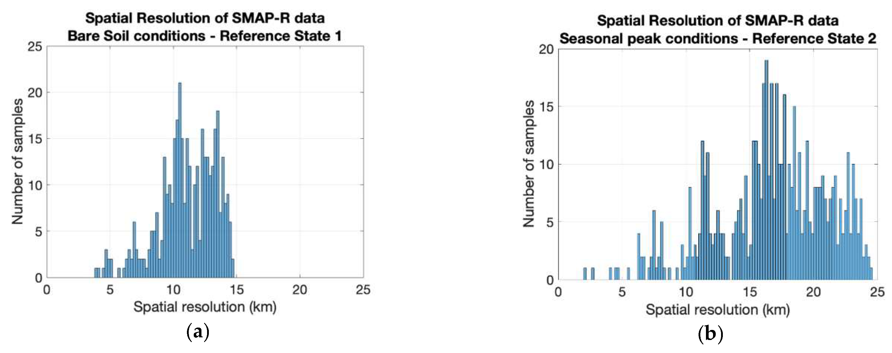
Figure 2.
Site selected: (a) U.S. Department of Agriculture (USDA) National Agricultural Statistics Service (NASS) [28] map showing the corn for all purposes planted in 2017, the red box indicating the specific area under study; (b) graph showing the total number of acres planted in consecutive years (2017 and 2018 show similar numbers; 2019 shows an increase); (c) stages of growth of a corn plant ([29], University of Illinois Extension program); and three images illustrating the agricultural landscape at different moments of the season; (d) terrain preparation for plantation (bare soil); (e) Vegetative-stage soybean planted and growing (high VWC, increasing height, and VOP); (f) soybean at the end of the season (low VWC, maximum height, medium VOP) being harvested (a layer of dried harvesting leftovers, low VWC, low VOP).


Figure 3.
Block diagram of the methodology implemented to assess the sensitivity of SMAP-R signals to crop growth parameters. The methodology is divided into three steps: SMAP-R data preparation, ancillary information use, and sensitivity analysis of SMAP-R signals to VWC, VOP, NDVI, and crop height. All datasets are gridded to the same 9 km × 9 km resolution. DDM, delay-Doppler maps; PR, polarimetric ratio; SM, soil moisture.

Figure 4.
Two-state analysis strategy: (a) corresponds to the PR values for bare soil state, and (b) corresponds to the PR values for the peak season state.
Figure 4.
Two-state analysis strategy: (a) corresponds to the PR values for bare soil state, and (b) corresponds to the PR values for the peak season state.

Figure 5.
Crop type map developed from the USDA NASS CropScape–Cropland Data database showing the predominant corn type in pixels of 9 × 9 km, matching SMAP official product spatial resolution [30].
Figure 5.
Crop type map developed from the USDA NASS CropScape–Cropland Data database showing the predominant corn type in pixels of 9 × 9 km, matching SMAP official product spatial resolution [30].

Figure 6.
Roughness information: SMAP ancillary product for surface roughness (static product).
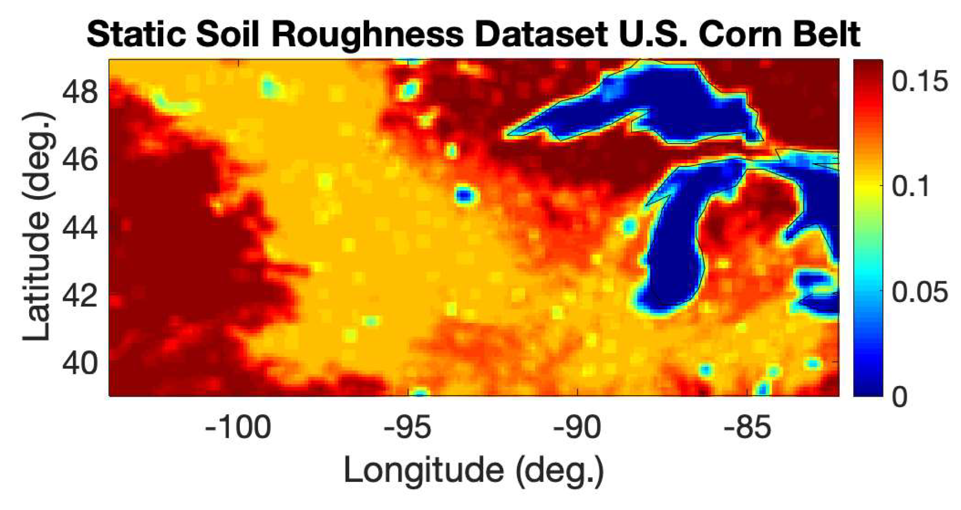
Figure 7.
Roughness information: (a) roughness mask built from low variability low roughness areas in Figure 6a and (b) masked predominant crop type information.
Figure 7.
Roughness information: (a) roughness mask built from low variability low roughness areas in Figure 6a and (b) masked predominant crop type information.

Figure 8.
Monthly soil moisture information for the 2017 season in the U.S. Corn Belt.
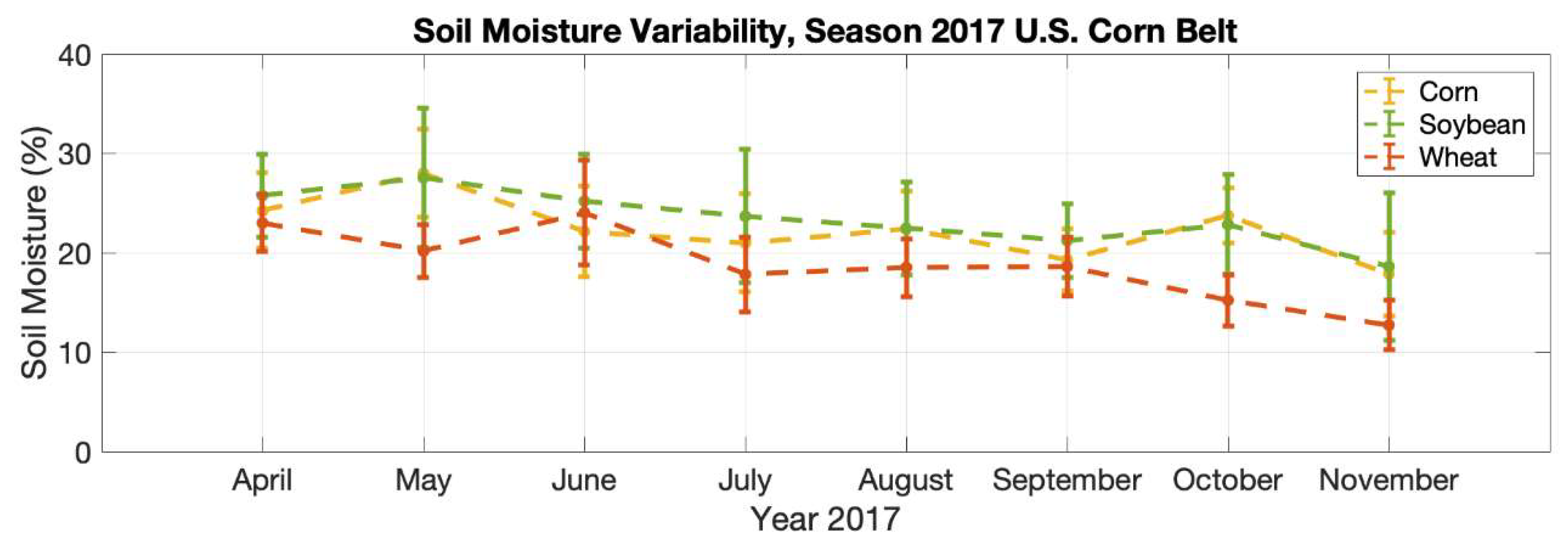
Figure 9.
Monthly crop NDVI information for the 2017 season in the U.S. Corn Belt.
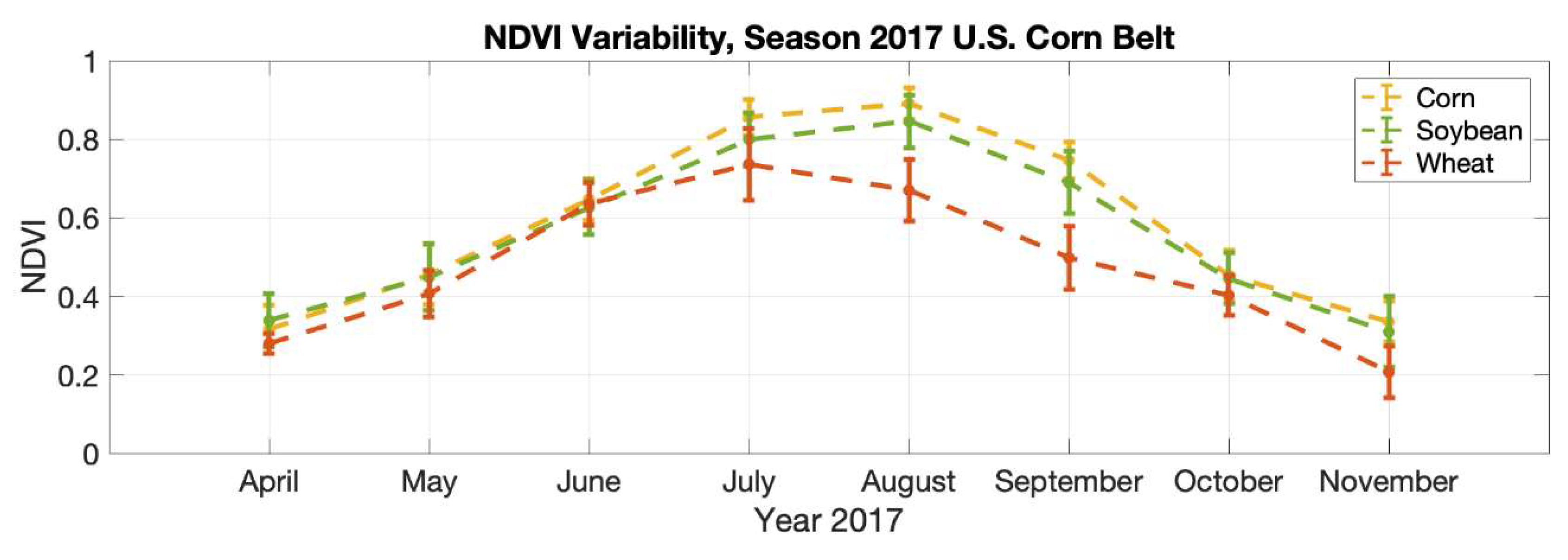
Figure 10.
Monthly crop condition information for the 2017 season in the U.S. Corn Belt: (a) SMAP ancillary product for VWC and (b) SMAP ancillary product for VOP.
Figure 10.
Monthly crop condition information for the 2017 season in the U.S. Corn Belt: (a) SMAP ancillary product for VWC and (b) SMAP ancillary product for VOP.

Figure 11.
Block diagram of the methodology implemented to estimate crop height monthly means.
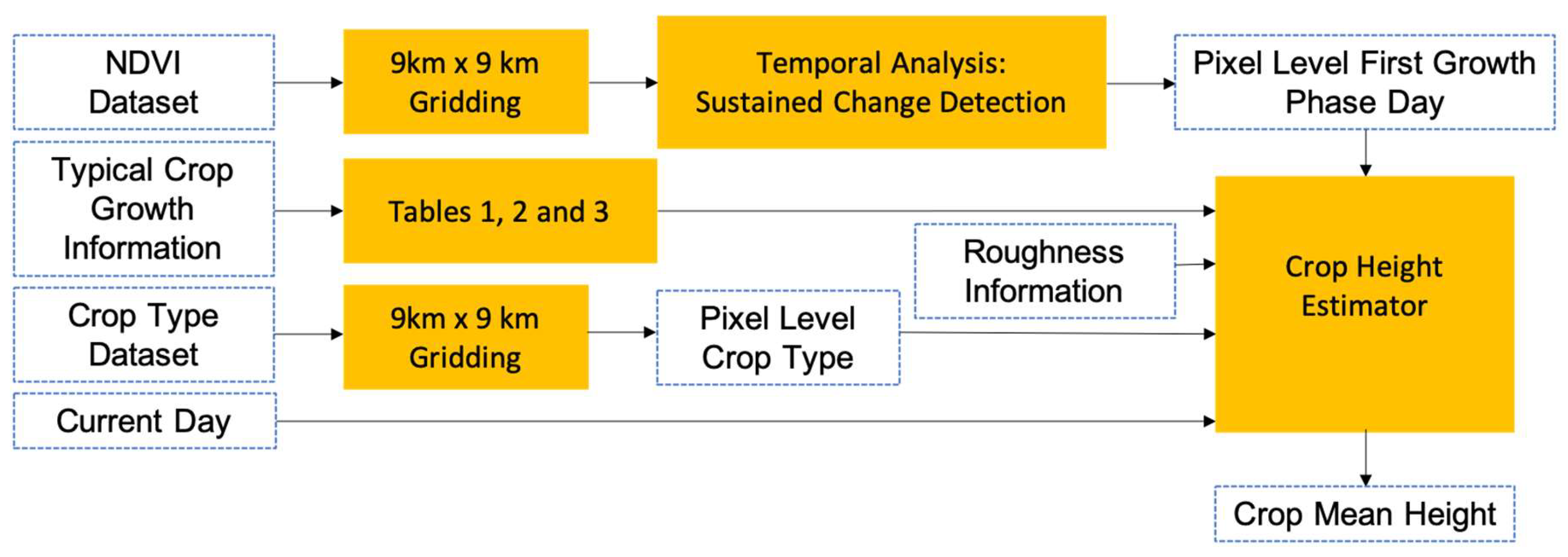
Figure 12.
Crop height information for the 2017 season in the U.S. Corn Belt. Note that the monthly mean of the estimated crop height is already filtered using roughness information to the area of low variability, low roughness area shown in Figure 4b.
Figure 12.
Crop height information for the 2017 season in the U.S. Corn Belt. Note that the monthly mean of the estimated crop height is already filtered using roughness information to the area of low variability, low roughness area shown in Figure 4b.

Figure 13.
Sample distribution for SM ranges of (a) [10–15]%, (b) [15–20]%, (c) [20–25]%, (d) [25–30]%, and (e) [30–35]%. Roughness mask applied to ensure low variability of low roughness values.
Figure 13.
Sample distribution for SM ranges of (a) [10–15]%, (b) [15–20]%, (c) [20–25]%, (d) [25–30]%, and (e) [30–35]%. Roughness mask applied to ensure low variability of low roughness values.

Figure 14.
PR seasonal variations (mean and std) for the SM range of (a) [15–20]% and (b) [25–30]%. Roughness mask applied to ensure the low variability of low roughness values.
Figure 14.
PR seasonal variations (mean and std) for the SM range of (a) [15–20]% and (b) [25–30]%. Roughness mask applied to ensure the low variability of low roughness values.

Figure 15.
Analysis of the dependence of PR on SM for (a) April (mostly bare soil, planting season), (b) June (growing stage, variability of heights for the same crop type), (c) August (season peak, plants at maximum height), and (d) November (after harvesting, the field contains residues and stalks from both corn and soybean left on the field after harvesting).
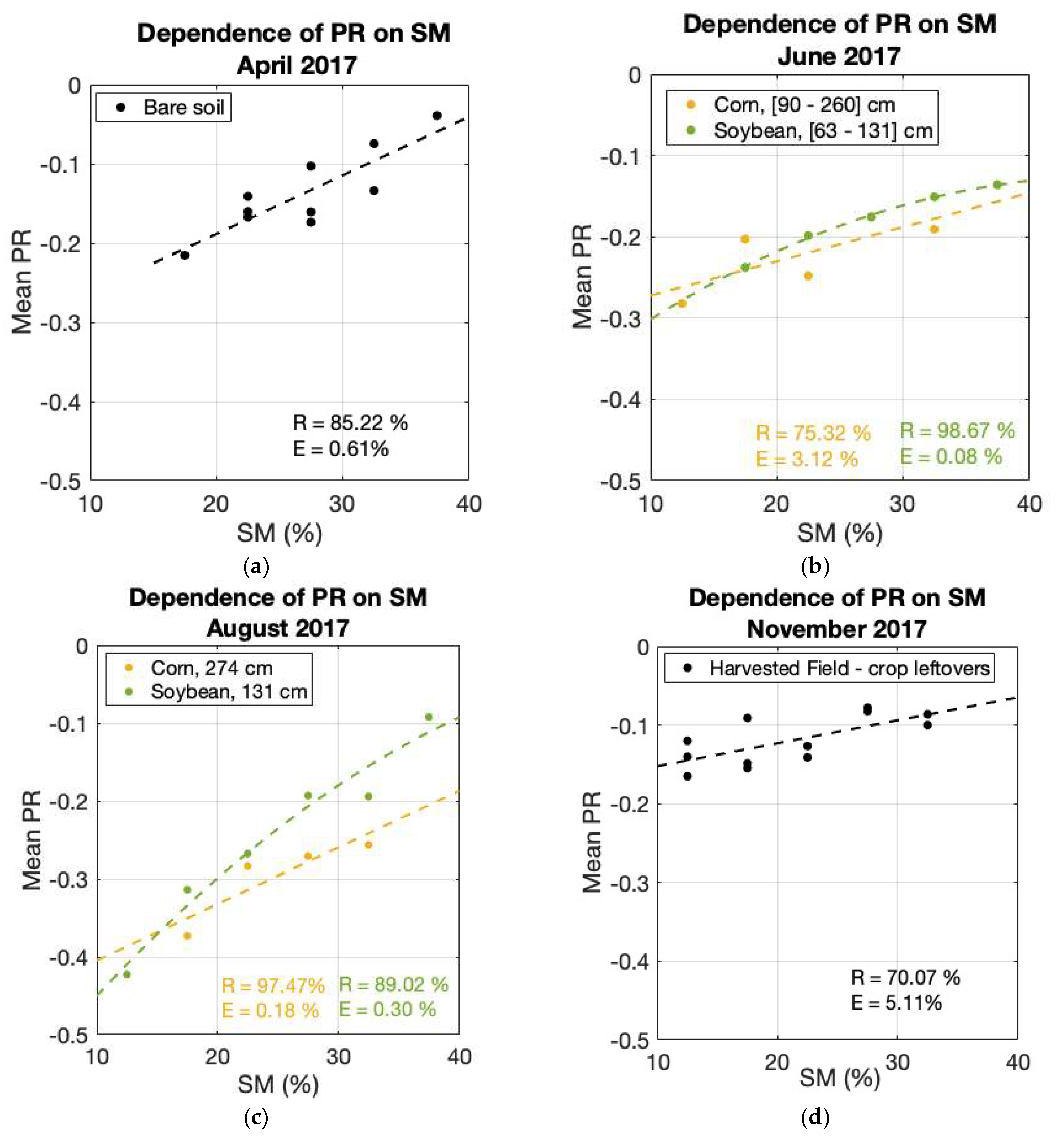
Figure 16.
PR dependency on crop height. Crop height information for the 2017 season in the U.S. Corn Belt obtained from the methodology explained through Figure 11. SMAP-R data analyzed contain corn and soybean for the SM range of [15–20]%.
Figure 16.
PR dependency on crop height. Crop height information for the 2017 season in the U.S. Corn Belt obtained from the methodology explained through Figure 11. SMAP-R data analyzed contain corn and soybean for the SM range of [15–20]%.

Figure 17.
PR dependency on VWC. VWC information for the 2017 season in the U.S. Corn Belt obtained from ancillary products stored in the SMAP SM official product [3]. SMAP-R data analyzed for (a) corn and (b) soybean.
Figure 17.
PR dependency on VWC. VWC information for the 2017 season in the U.S. Corn Belt obtained from ancillary products stored in the SMAP SM official product [3]. SMAP-R data analyzed for (a) corn and (b) soybean.
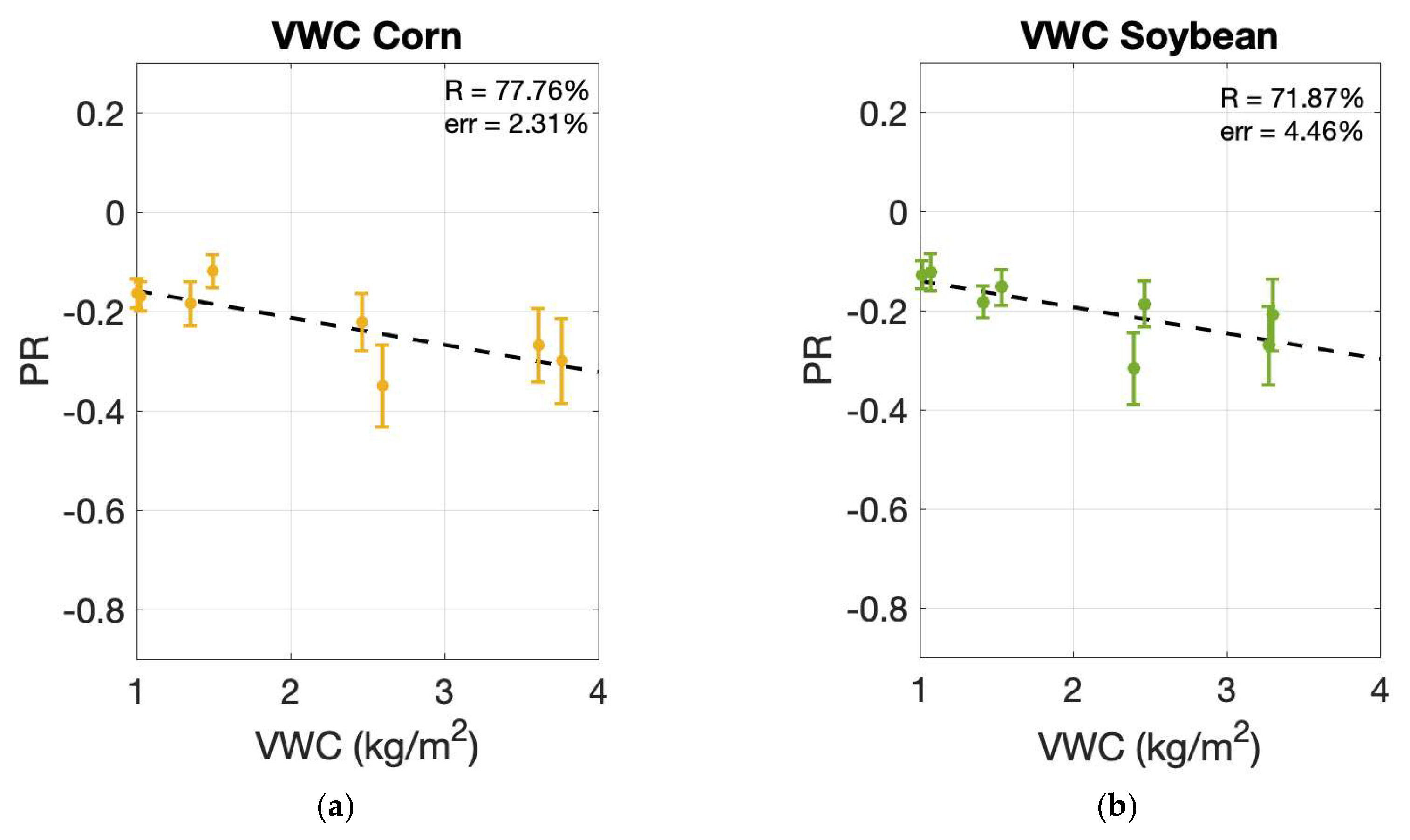
Figure 18.
PR dependency on VOP. VOP information for the 2017 season in the U.S. Corn Belt obtained from ancillary products within the SMAP SM official product [3]. SMAP-R data analyzed for (a) corn and (b) soybean.
Figure 18.
PR dependency on VOP. VOP information for the 2017 season in the U.S. Corn Belt obtained from ancillary products within the SMAP SM official product [3]. SMAP-R data analyzed for (a) corn and (b) soybean.
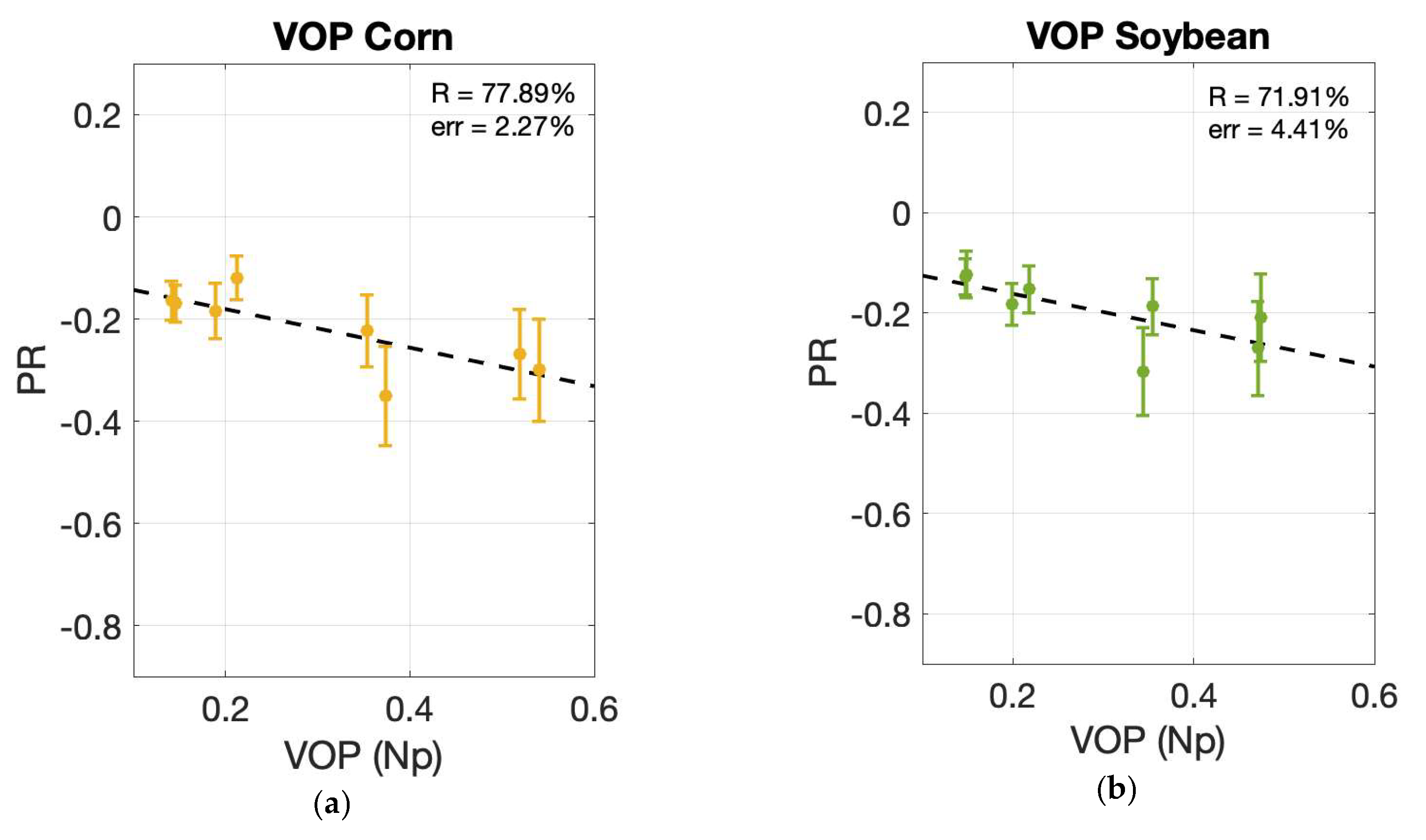
Figure 19.
PR dependency on NDVI. NDVI information for the 2017 season in the U.S. Corn Belt obtained from [34]. SMAP-R data analyzed for (a) corn and (b) soybean.
Figure 19.
PR dependency on NDVI. NDVI information for the 2017 season in the U.S. Corn Belt obtained from [34]. SMAP-R data analyzed for (a) corn and (b) soybean.


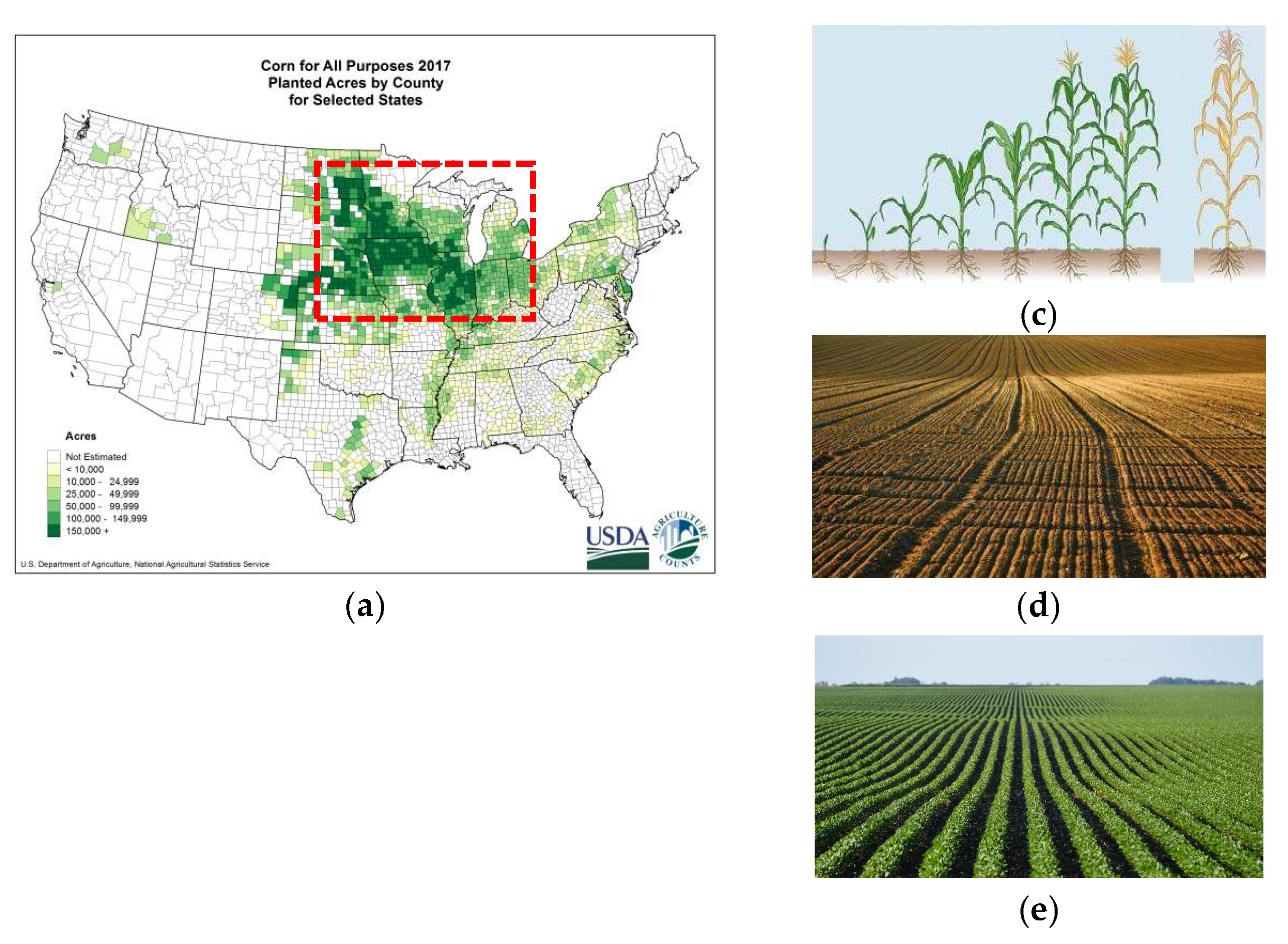
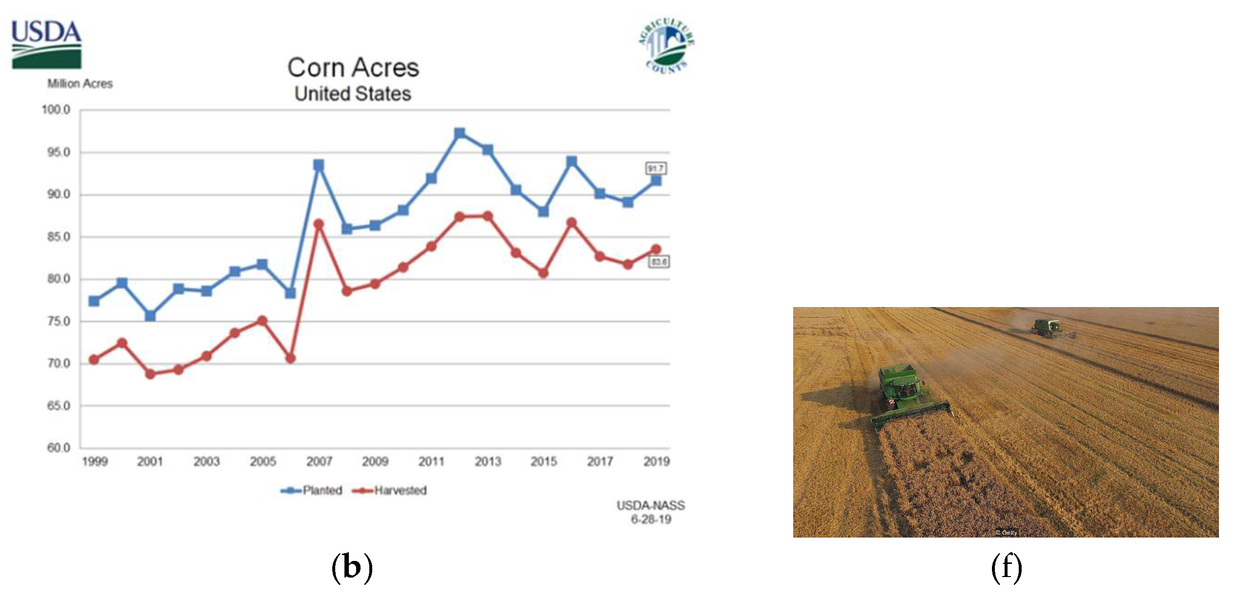
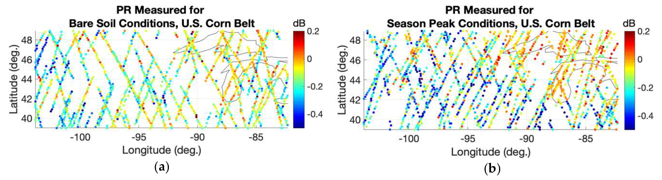
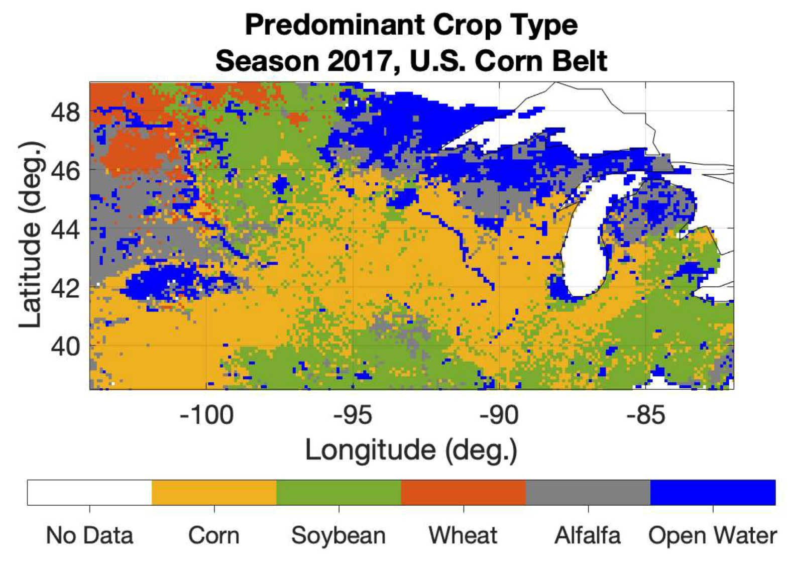
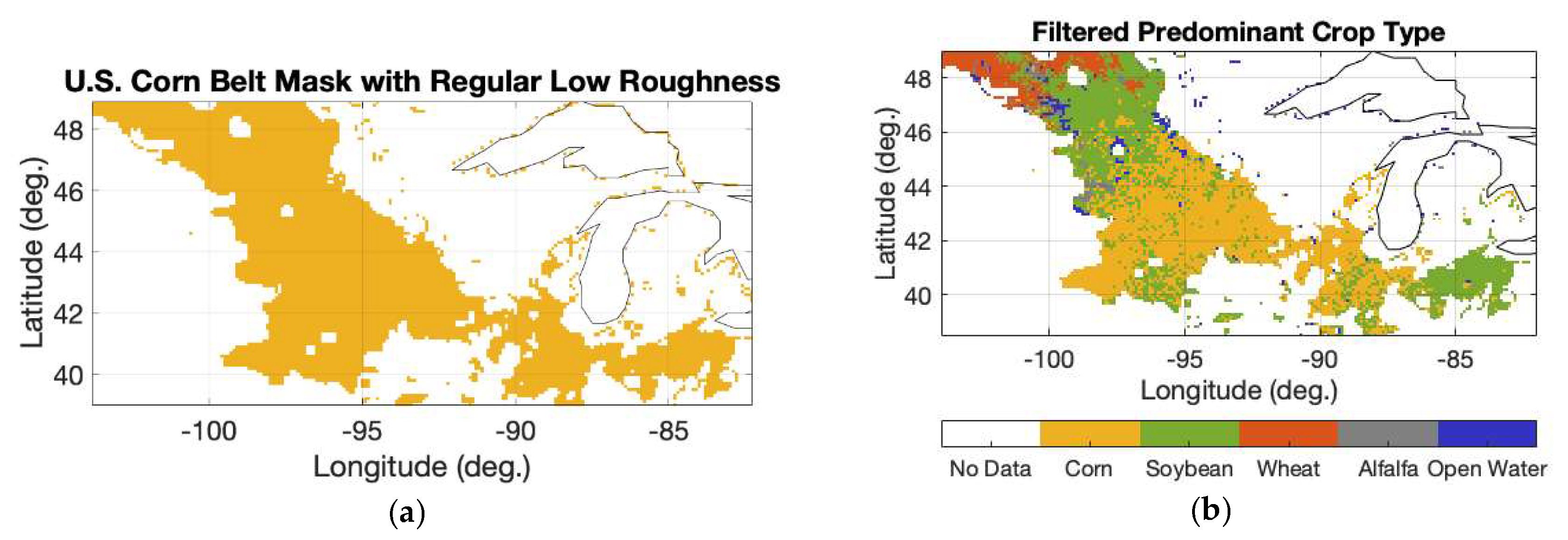
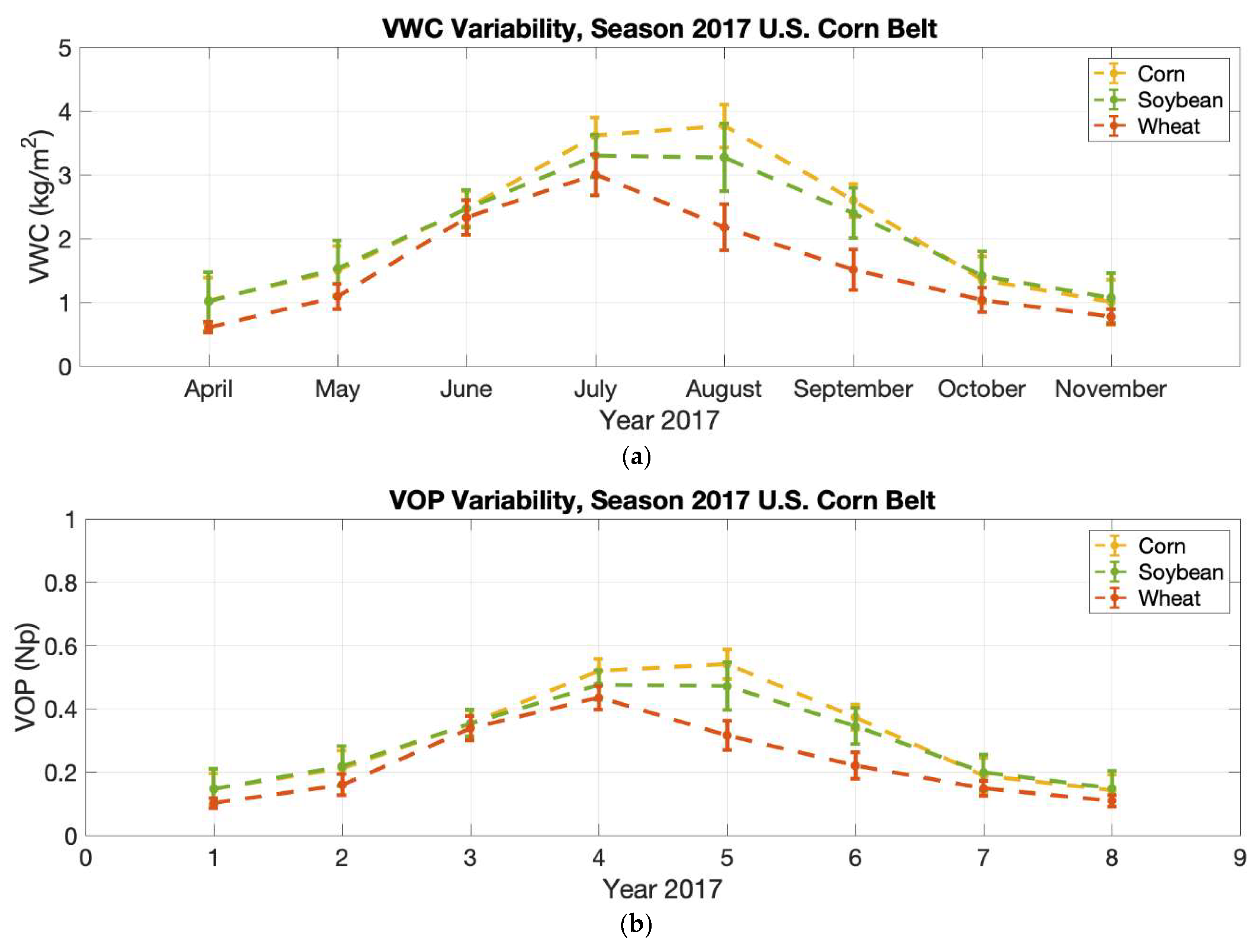
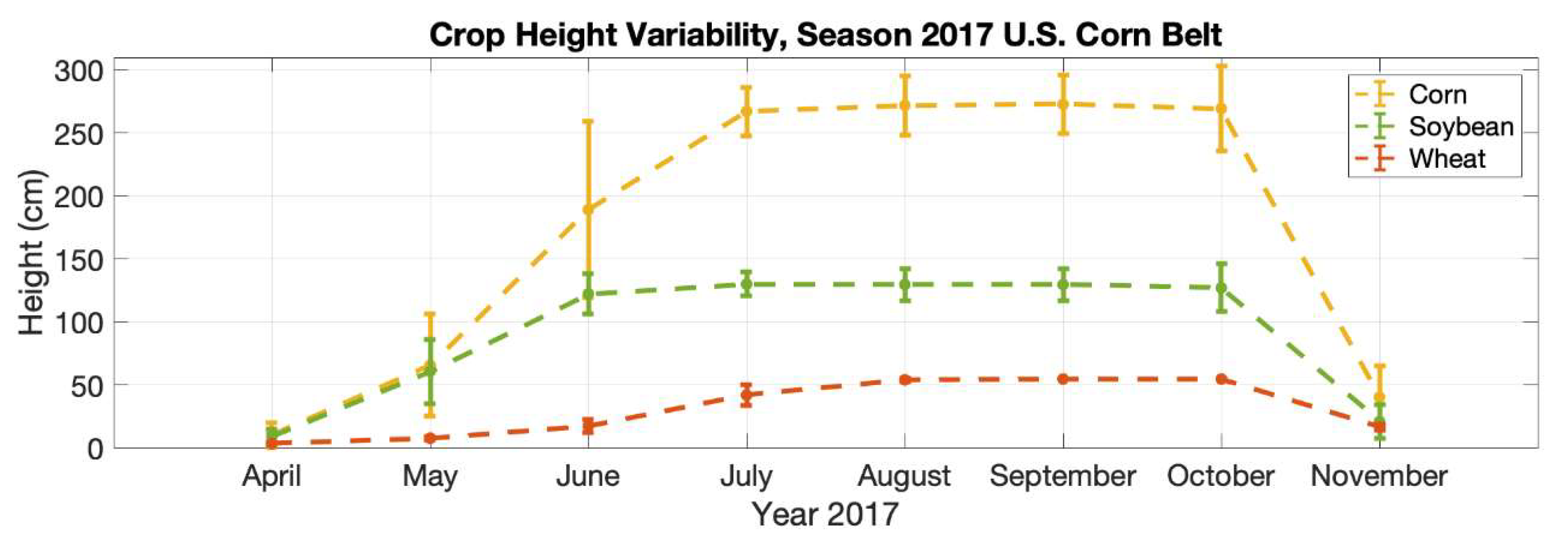
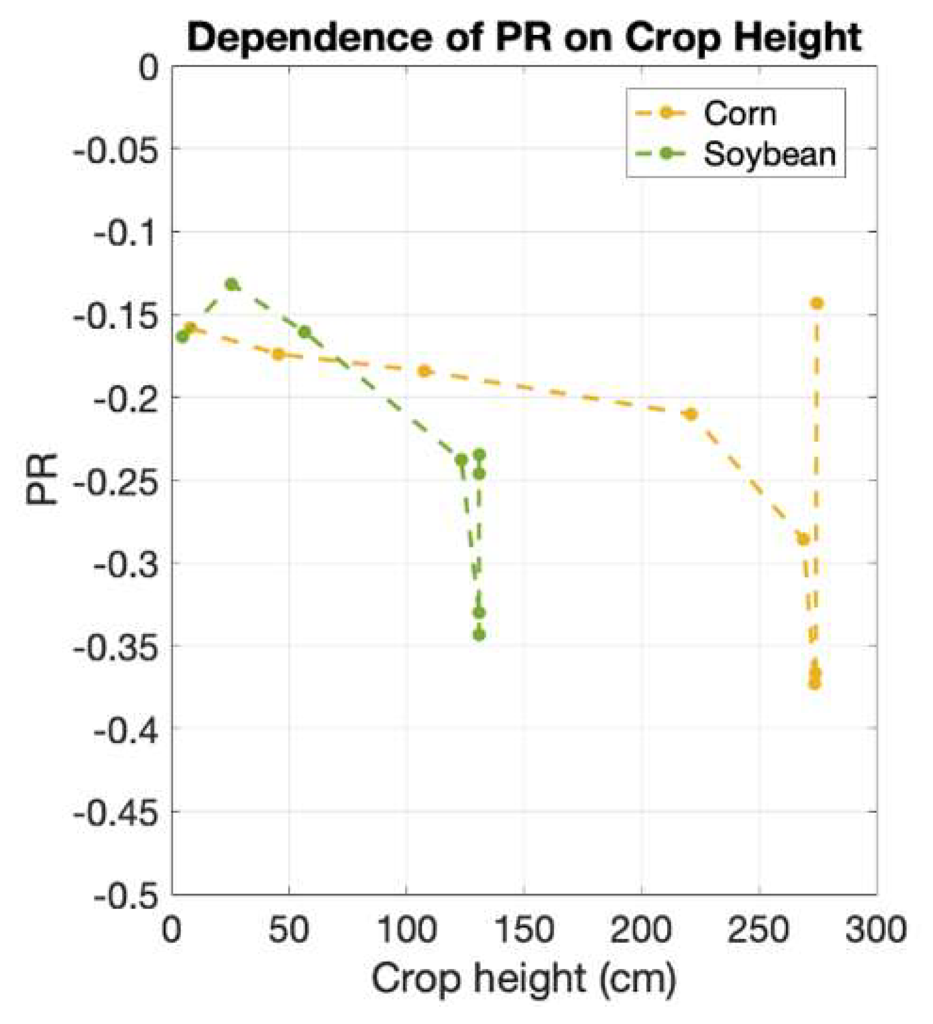
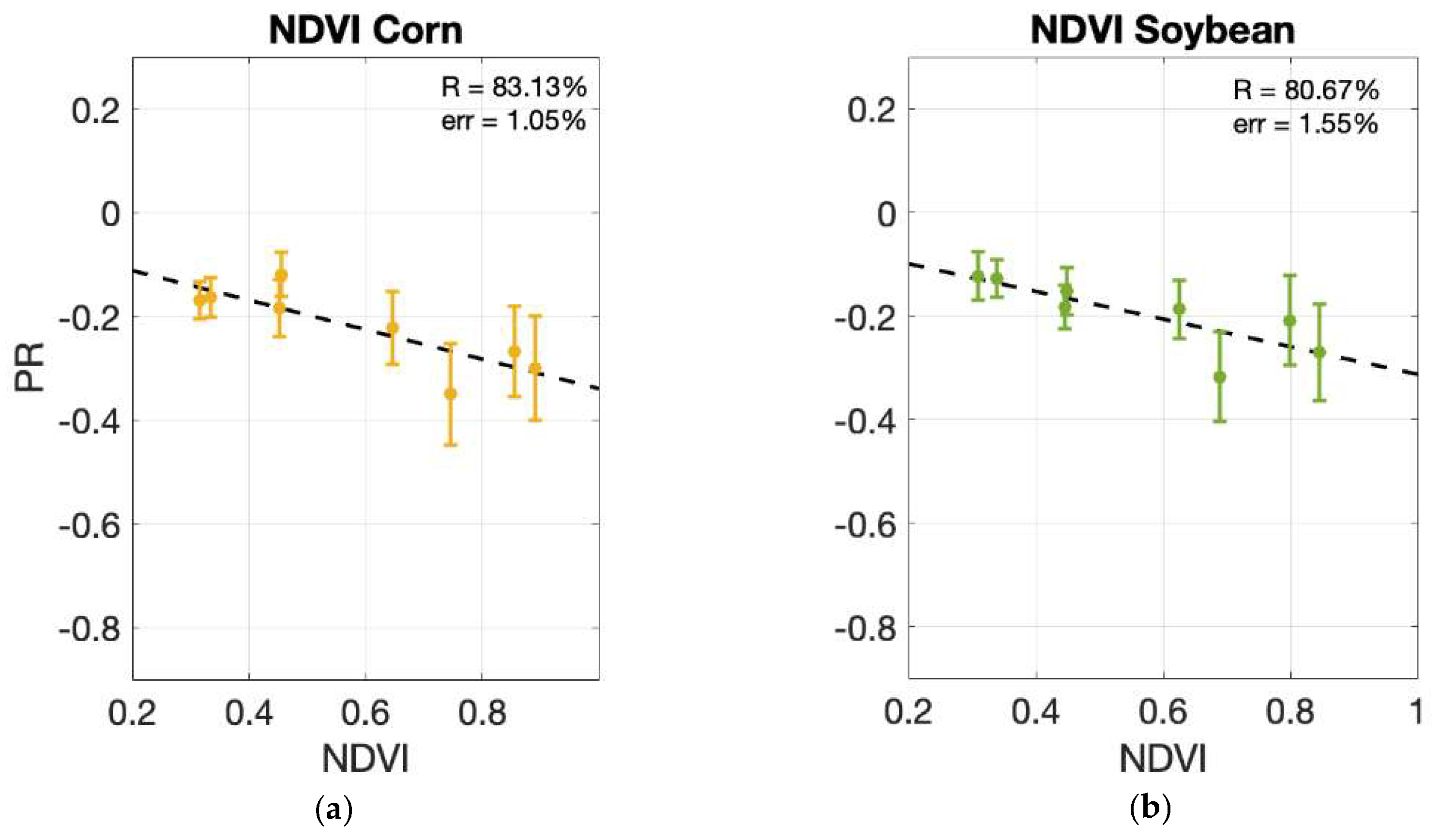
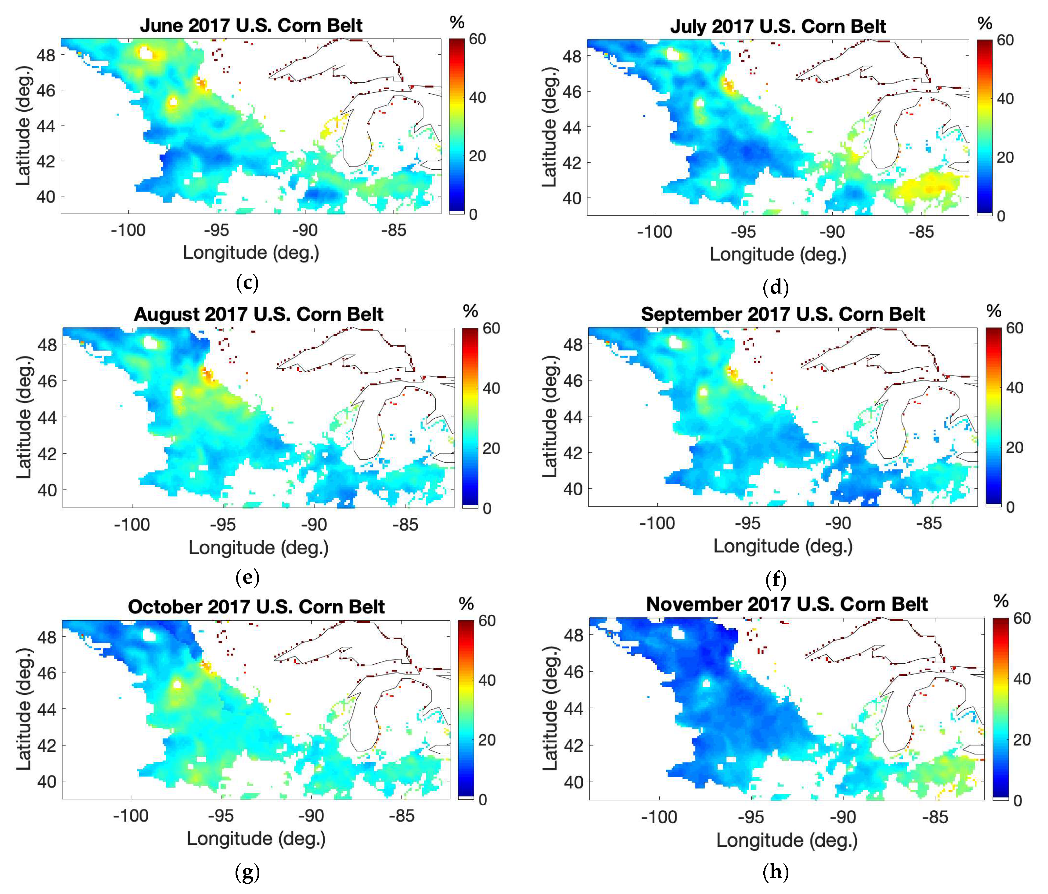
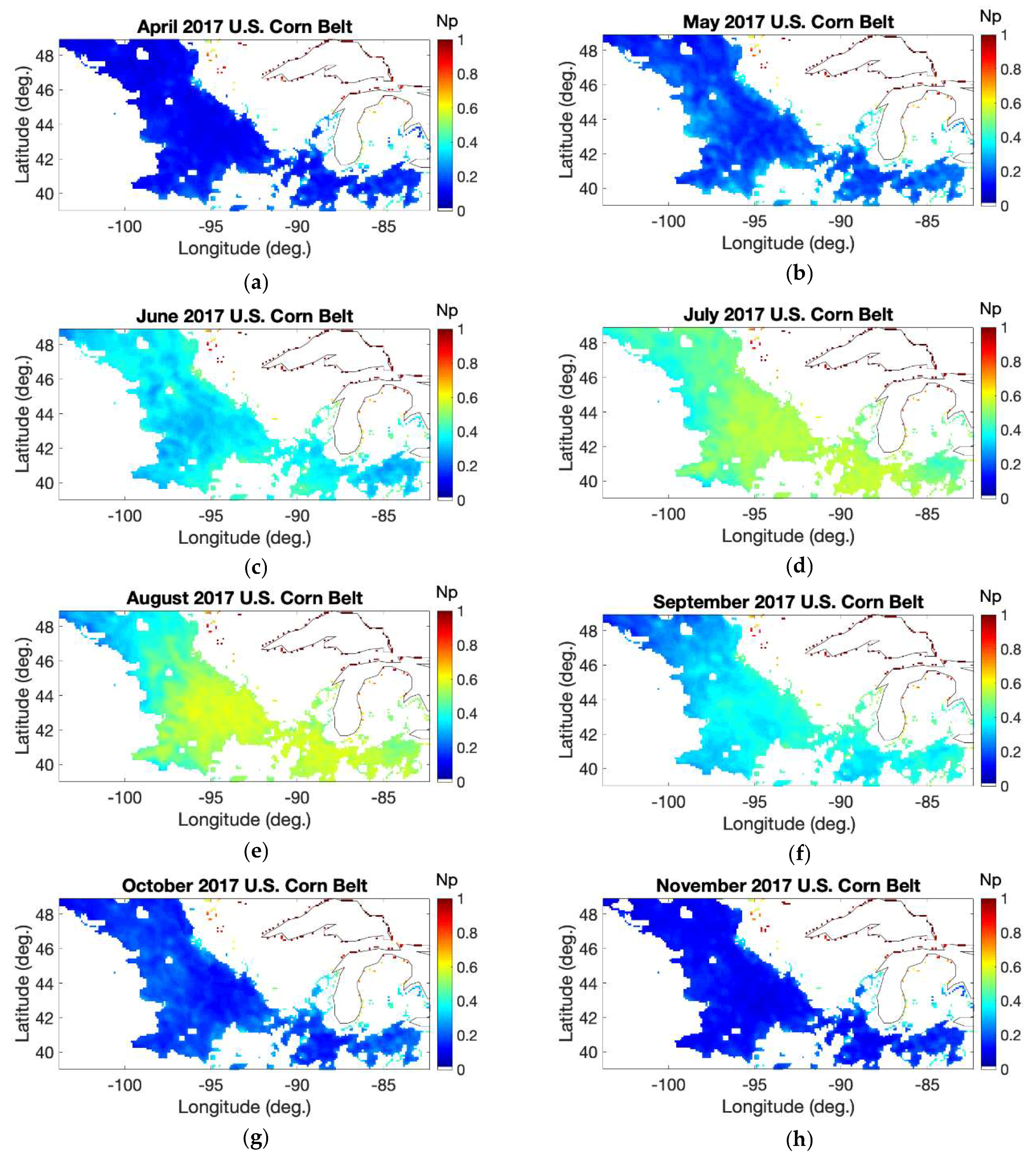
Table 1.
Corn height based on growth stage. Based on the growth observed reported in [41] for the ground-truth of corn field. Vx = Vegetative stages, Rx = Reproductive stages.
Table 1.
Corn height based on growth stage. Based on the growth observed reported in [41] for the ground-truth of corn field. Vx = Vegetative stages, Rx = Reproductive stages.
| Growth Stage | Height (cm) | Days |
|---|---|---|
| Emergence (VE) | 0 | 0 |
| 1 leaves (V1) | 5 | 7 |
| 5 leaves (V5) | 14 | 14 |
| 8 leaves (V8) | 48 | 28 |
| 12 leaves (V12) | 89 | 42 |
| 16 leaves (V16) | 125 | 56 |
| 18/21 leaves (V18/V21) Tassel and silk (VT) | 250 | 66 |
| Reproductive stages (R1-R5) | 260–275 | 70–120 |
| Maturity (R6) | 275 | 126 |
Table 2.
Wheat height based on growth stage. Based on the growth observed reported in [42] for the ground-truth of wheat field.
Table 2.
Wheat height based on growth stage. Based on the growth observed reported in [42] for the ground-truth of wheat field.
| Growth Stage | Height (cm) | Days |
|---|---|---|
| Emergence (1) | 0 | 0 |
| Tillering (2) | 3 | 7 |
| Tillers formed (3) | 6 | 25 |
| Tillers erect (4) | 9 | 50 |
| Tillers strong (5) | 12 | 60 |
| First node (6) | 16 | 70 |
| Second node (7) | 21 | 75 |
| Last leaf (8) | 27 | 85 |
| Ligule visible (9) | 35 | 90 |
| Boot, head swollen (10) | 44 | 98 |
| Heading (10.1) | 47 | 105 |
| Flowering (10.5) | 51 | 110 |
| Ripening (11) | 55 | 125 |
Table 3.
Soybean height based on growth stage. From VE to V5, soybean moves to a new V stage every 6 days and grows about 1.9 cm/day. From R1 to R6, soybean moves to a new stage every 4 days and grows about 4 cm per day [43]. Vx = Vegetative stages, Rx = Reproductive stages.
Table 3.
Soybean height based on growth stage. From VE to V5, soybean moves to a new V stage every 6 days and grows about 1.9 cm/day. From R1 to R6, soybean moves to a new stage every 4 days and grows about 4 cm per day [43]. Vx = Vegetative stages, Rx = Reproductive stages.
| Growth Stage | Height (cm) | Days |
|---|---|---|
| Emergence (VE) | 0 | 0 |
| Unrolled unifoliate (VC) | 3 | 7 |
| 1 trifoliate developed (V1) | 8.65 | 13 |
| 2 trifoliate developed (V2) | 18.18 | 19 |
| 3 trifoliate developed (V3) | 27.71 | 25 |
| 4 trifoliate developed (V4) | 37.23 | 31 |
| 5/6 trifoliate developed (V5/V6) | 46.76 | 37 |
| Flowering (R1-R2) | 53.11–129 | 41–57 |
| Pod development (R3-R4) | ||
| Seed filling (R5-R6) | ||
| Maturity (R7-R8) | 131 | 61–100 |
Table 4.
PR sensitivity to VWC, with the uncertainty of the estimations for corn and soybean crop type. The green dashed box highlights the SM ranges with a statistically significant number of samples. R is the correlation [45]; E is the probability of R being random [45]; S is the sensitivity; and U is the uncertainty. The VWC maximum range is [0–4] kg/m2.

Table 5.
PR sensitivity to VOP, with the uncertainty of the estimations for corn and soybean crop type. The green dashed box highlights the SM ranges with a statistically significant number of samples R is the correlation [45]; E is the probability of R being random [45]; S is the sensitivity; and U is the uncertainty. The VOP maximum range is [0 to 1] Np.

Table 6.
PR sensitivity and NDVI uncertainty of the estimations for corn and soybean crop type. The green dashed box highlights the SM ranges with a statistically significant number of samples. R is the correlation [45]; E is the probability of R being random [45]; S is the sensitivity; and U is the uncertainty. The NDVI maximum range is [0 to 1].

© 2020 by the authors. Licensee MDPI, Basel, Switzerland. This article is an open access article distributed under the terms and conditions of the Creative Commons Attribution (CC BY) license (http://creativecommons.org/licenses/by/4.0/).
Share and Cite
MDPI and ACS Style
Rodriguez-Alvarez, N.; Misra, S.; Morris, M. The Polarimetric Sensitivity of SMAP-Reflectometry Signals to Crop Growth in the U.S. Corn Belt. Remote Sens. 2020, 12, 1007. https://0-doi-org.brum.beds.ac.uk/10.3390/rs12061007
AMA Style
Rodriguez-Alvarez N, Misra S, Morris M. The Polarimetric Sensitivity of SMAP-Reflectometry Signals to Crop Growth in the U.S. Corn Belt. Remote Sensing. 2020; 12(6):1007. https://0-doi-org.brum.beds.ac.uk/10.3390/rs12061007
Chicago/Turabian StyleRodriguez-Alvarez, Nereida, Sidharth Misra, and Mary Morris. 2020. "The Polarimetric Sensitivity of SMAP-Reflectometry Signals to Crop Growth in the U.S. Corn Belt" Remote Sensing 12, no. 6: 1007. https://0-doi-org.brum.beds.ac.uk/10.3390/rs12061007
Note that from the first issue of 2016, this journal uses article numbers instead of page numbers. See further details here.