A Deep Convolutional Neural Network for Oil Spill Detection from Spaceborne SAR Images


1
Ocean Remote Sensing Institute, Ocean University of China, Qingdao 266003, China
2
Laboratory for Regional Oceanography and Numerical Modeling, Pilot National Laboratory for Marine Science and Technology, Qingdao 266237, China
*
Author to whom correspondence should be addressed.
Remote Sens. 2020, 12(6), 1015; https://0-doi-org.brum.beds.ac.uk/10.3390/rs12061015
Submission received: 3 February 2020
/
Revised: 19 March 2020
/
Accepted: 19 March 2020
/
Published: 22 March 2020
(This article belongs to the Special Issue Synthetic Aperture Radar Observations of Marine Coastal Environments)
Abstract
:Classification algorithms for automatically detecting sea surface oil spills from spaceborne Synthetic Aperture Radars (SARs) can usually be regarded as part of a three-step processing framework, which briefly includes image segmentation, feature extraction, and target classification. A Deep Convolutional Neural Network (DCNN), named the Oil Spill Convolutional Network (OSCNet), is proposed in this paper for SAR oil spill detection, which can do the latter two steps of the three-step processing framework. Based on VGG-16, the OSCNet is obtained by designing the architecture and adjusting hyperparameters with the data set of SAR dark patches. With the help of the big data set containing more than 20,000 SAR dark patches and data augmentation, the OSCNet can have as many as 12 weight layers. It is a relatively deep Deep Learning (DL) network for SAR oil spill detection. It is shown by the experiments based on the same data set that the classification performance of OSCNet has been significantly improved compared to that of traditional machine learning (ML). The accuracy, recall, and precision are improved from 92.50%, 81.40%, and 80.95% to 94.01%, 83.51%, and 85.70%, respectively. An important reason for this improvement is that the distinguishability of the features learned by OSCNet itself from the data set is significantly higher than that of the hand-crafted features needed by traditional ML algorithms. In addition, experiments show that data augmentation plays an important role in avoiding over-fitting and hence improves the classification performance. OSCNet has also been compared with other DL classifiers for SAR oil spill detection. Due to the huge differences in the data sets, only their similarities and differences are discussed at the principle level.

1. Introduction
Oil spills on the sea surface have become major environmental and public safety issues that cannot be ignored. With the widespread attention of the development and utilization of marine resources, the marine transportation industry and the offshore oil and gas industry have developed rapidly in recent years. However, oil spill events from ships and offshore oil platforms frequently occur in various seas all over the world, which results in huge ecological and property losses [1].
Oil spill accidents often occur in areas with complex marine environments. Therefore, it is hard to directly enter the polluted area to clean or make observations in the early stage. Such events usually last days [2], weeks [3], or even months [4], so continuous observations are needed to study the spreading of oil spills and how much they impact environmental safety [5]. The Synthetic Aperture Radar (SAR) can be regarded as a sensor used to measure the sea surface roughness. Sea surfaces covered with oil films appear dark in SAR images because the capillary waves and short gravity waves that contribute to the sea surface roughness are damped by the surface tension of oil films [6]. This gives spaceborne SARs the possibility to monitor oil spills in large areas in a highly efficient and relatively cheap way. Compared with spaceborne optical and infrared sensors, spaceborne SARs have obvious advantages in marine oil spill detection because they yield data independent of the time of day and weather conditions [7].
However, many oceanic and atmospheric phenomena other than oil spills may also reduce the sea surface roughness and appear dark in SAR images. A typical processing framework for automatic SAR oil spill detection usually contains roughly three steps. The first step is to obtain dark patches from SAR images by an image segmentation algorithm, the second step is to extract features from these dark patches to form a feature vector set, and the third step is to train a classifier using the feature vector set. The obtained classifier can then be used to identify oil spills and lookalikes in the dark patches extracted from SAR images by the same segmentation algorithm [8].
In the last two decades, many classification algorithms have been developed for SAR oil spill detection based on traditional machine learning (ML), such as the linear model [9], Decision Trees [10,11,12], Artificial Neural Networks (ANNs) [13,14,15,16,17], Support Vector Machines (SVMs) [18,19,20], Bayesian Classifiers [21,22], Ensemble Learning [14], and so on. These methods have demonstrated their own effectiveness based on their respective data. However, we can only evaluate these algorithms perceptually, and it is difficult to directly compare their classification performance indicators due to the various data sets they use.
What the ML approaches essentially do is seek a statistically optimal decision surface in the feature space, and mathematically, it comes down to an optimization problem. For a specific classification problem, the more data there is, the more stable the statistical characteristics, and the more generalizable the obtained decision surface and corresponding classification performance indicators in the problem domain following the same statistical characteristics. In this sense, the classification performance indicators of [14] are relatively reliable, because its data set includes 4843 oil spills and 18,925 lookalikes extracted from 336 SAR images, which is the largest data set used by the ML classifiers mentioned above. In [14], an Area weighted Adaboost Multi-Layer Perceptron (AAMLP) was proposed, which achieved a classification accuracy, recall, and precision of 92.50%, 81.40%, and 80.95%, respectively.
In recent years, some Deep Learning (DL) methods have been used for SAR oil spill detection. Huang et al. [23] proposed a three-layer Deep Belief Network (DBN) with a Gray-Level Co-occurrence Matrix (GLCM) as the input to distinguish whether a piece of SAR sample image is oil spill, lookalike, or sea water. Here, the GLCM was calculated from the sample image. The DBN was trained with 240 samples and obtained a recognition rate of 91.25%. Guo et al. [24] used a Convolutional Neural Network (GCNN) to distinguish crude oil, plant oil, and oil emulsion. The GCNN was trained with 5400 samples and obtained a recognition rate of 91.33%. Gallego et al. [25] designed a two-stage Convolutional Neural Network (TSCNN) to classify the pixels of a Side-Looking Airborne Radar (SLAR) image into ship, oil spill, coastal, or sea water. This is actually a segmentation algorithm since it works at a pixel level. The TSCNN achieved an accuracy of 98%, recall of 73%, and precision of 52% for oil spill detection based on a data set of 23 SLAR images. Gallego et al. [26] proposed a very deep Residual Encoder-Decoder Network (RED-Net) to segment out the oil spill from SLAR, which obtained a recall value of 92.92%.
Although there is no accepted definition for how many layers constitute a "deep" learner, a typical deep network should typically include at least four or five layers [27]. From this point of view, the layers of the DL networks mentioned above are all relatively shallow. So far, we have not seen a DL network for SAR oil spill detection with more than seven weight layers (including convolutional layers and Fully Connected layers (FCs)). Seven is the layer number of LeNet—the first famous DL network [28]. The depth of the DL network is most likely related to the size of the data sets used. This issue will be discussed in Section 5.
In this paper, a Deep Convolutional Neural Network (DCNN) with a sufficient depth is proposed to classify SAR dark patches for oil spill detection as an upgrade solution of the AAMLP used in the automatic SAR oil spill detection system [14].
We will use the same data set as that of AAMLP to construct the proposed DCNN. Firstly, this data set is relatively large, and the number of samples can be increased sufficiently to support a deeper network through the data augmentation technique (see Section 5.4). Secondly, it provides a chance to compare the DL network with the traditional ML network based on the same relatively large data set (see Section 5.3).
At present, there are four main branches of DL architecture, namely the Auto-Encoder (AE), the Convolutional Neural Network (CNN), DBN, and the Recurrent Neural Network (RNN) [27]. Why CNN is chosen in the proposed network lies in the outstanding performance of several well-known CNNs, i.e., AlexNet [29], ZFNet [30], VGG-16, and VGG-19 [31], exhibited in the competition of the ImageNet Large Scale Visual Recognition Challenge (ILSVRC) from 2012 to 2014, and the successful application of CNNs in the SAR oil spill detection research mentioned above. Therefore, it can be expected that based on the same dark patch data set, a DL network with a better classification performance than that of the traditional ML network can be constructed. A distinctive capability of CNN is that it can learn to extract features directly from the data itself through training, while traditional ML methods require "hand-crafted" features [27]. It can be seen in Section 5.5 that the distinguishability of the features automatically extracted by the proposed DCNN in this paper is significantly better than the 77 hand-crafted features used by AAMLP. This is an important reason why the classification performance of DCNN is superior to that of ML methods.
The flowchart employed to build the proposed DCNN is shown in Figure 1. First, the data set of AAMLP is used to carry out transfer learning in three candidate networks, and then, the best one is taken as the basic network architecture. Next, the network architecture and hyperparameters are adjusted on this basis. The network no longer uses transfer learning, but is trained from scratch, because those adjustment procedures involve changes in both the architecture and hyperparameters. We refer to the resulting network as the Oil Spill Convolutional Network (OSCNet). It should be noted that data augmentation is only applied to the training data set. We believe that it is more objective to evaluate the performance of the classifier using the original test data set.
The rest of the paper is organized as follows: Section 2 introduces the source and composition of the SAR oil spill dark patch data set and the relevant preprocessing methods; in Section 3, the basic network architecture is selected from three candidate DCNNs by transfer learning; Section 4 describes how the architecture is determined and how the hyperparameters are adjusted for establishing the OSCNet; in Section 5, the experimental results are demonstrated and analyzed, and the comparisons of OSCNet with other classifiers are made; finally, the conclusion and outlooks are given in Section 6.
2. Data
2.1. Data Set
In 2011, a serious oil spill accident occurred in the Bohai Bay of China, which polluted more than 840 km2 of sea water and forced the closure of multiple offshore oil and gas platforms. In 2016, an operational automatic SAR oil spill detection system, named CNOOCOM for the China National Offshore Oil Corporation (CNOOC), was developed by the Ocean Remote Sensing Institute, Ocean University of China (ORSI/OUC) [14]. The system implemented the automatic downloading or manual acquisition of multi-source SAR data, sea-land segmentation, image preprocessing, dark patch extraction by an adaptive threshold segmentation, post-processing of segmentation, feature extraction of dark patches, AAMLP classifiers, and so on. Once an SAR image is received, the system automatically generates a thematic map and reports oil spills found on the SAR image after the series of processing steps described above within about 5 min. The data set used for training AAMLP is composed of 23,768 dark patches extracted from 336 multi-source SAR images by an adaptive threshold segmentation algorithm based on multi-scale background estimation. These dark patches were labeled as 4843 oil slicks and 18,925 lookalikes through an iterative procedure which combined machine and manual classification. The data set covers a large spatial and temporal range, as shown in Table 1. Additionally, many known big oil spill events, such as the BP oil spill and Bohai oil spill, are included in the data set.
The dark patch generation algorithm is quite complicated and will be introduced in detail in another paper. However, in view of the fact that the data set in this paper is uniformly generated from 336 SAR images using the image segmentation program, it is necessary to briefly introduce the generation process.
First, this algorithm uses an iterative operation to estimate the image intensity component in the sea area as a function of the incident angle. Taking this component as a criterion, the trends of the image intensity with the angle can be eliminated to obtain many coarse dark patches. A series of moving windows with a decreasing size are used to gradually refine the boundary of the dark patches. A distinct advantage of this algorithm is that it is suitable for dark patches of different sizes. Finally, a connected area composed of dark pixels is considered as a single dark patch.
Since an oil spill usually appears as several disconnected dark patches and each one is considered independent, the number of oil spills established through this process is often greater than the number of oil spills identified by experts. Unfortunately, due to the inherent complexity of the SAR image, many small dark patches are inevitably introduced, making the number of dark patches extremely large. To reduce the large number of non-oil dark patches, the image segmentation program also includes a post-processing filtering chain based on simple rules. These rules must be loose enough to guarantee that oil spills will not be removed. Therefore, even with the existence of the filter chain, many non-oil dark patches are still retained. Some of them are not even lookalikes, but since they have become part of the data set, we also consider them as lookalikes. After many post-processing efforts, we successfully reduced the ratio of lookalikes to oil spills from about 100:1 to 3.9:1. This greatly reduced the imbalance of the data set.
As part of the automatic oil spill detection system, the classifier has to process all dark patches generated by the segmentation program when the system is running. Therefore, the data set used for training the classifier must involve all dark patches generated from the 336 images by the segmentation program, so as to ensure that the statistical characteristics of the data set are consistent with those of dark patches to be processed by the classifier in the future.
2.2. Input Size of DCNN
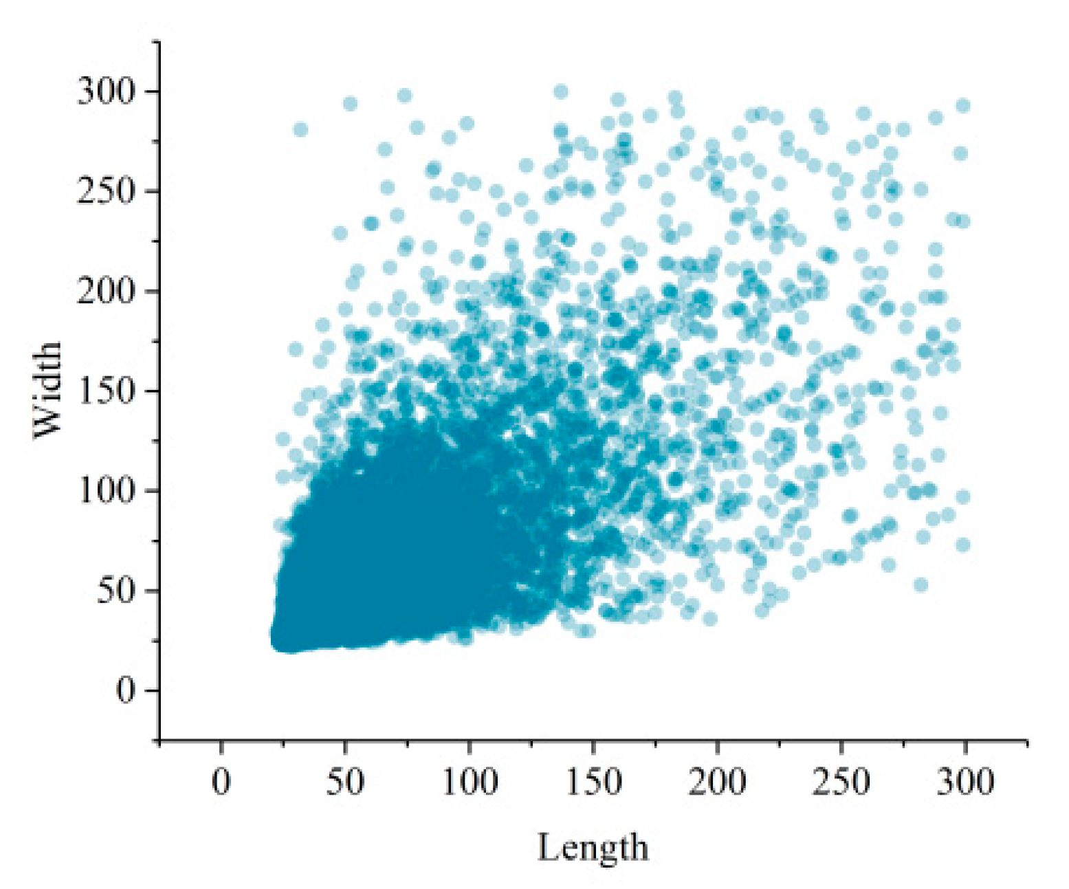
Each dark patch has to be re-sampled to a given size because the DCNN requires the size of the input image to be fixed [32]. The re-sampled operation will change the aspect ratio of the samples. In order to make the deformation as small as possible, we employed the input size of 64 × 64, which is close to the mean value of the sample size, as shown in Figure 2. This size was used for all DCNN experiments presented in this paper. The re-sampled operation is performed on-the-fly when a dark patch image is fed to the network during training or evaluating. This facilitates superimposing the samples on the original SAR image to visualize the classification results. In fact, the size of dark patches varies in a very wide range, but as the size increases, the number of dark patches decreases rapidly. The maximum size of an oil spill dark patch is 2136, corresponding to about 150km, which was extracted from a wide swath Envisat ASAR image acquired during the BP oil spill event in the Gulf of Mexico in 2010. In order to show the size distribution more clearly, only samples with a size of less than 300 are plotted.
2.3. Preprocessing
Data set preprocessing is divided into two parts: Data set proportion allocation and data augmentation. Data set proportion allocation is key to guaranteeing the data characteristics of dark patch samples and the ability of network generalization. It is also the basis for a comparison with AAMLP. Data augmentation is employed to maximize the advantage of our data set, without destroying the original data feature distribution, so that the network can avoid over-fitting.
2.3.1. Data Set Proportion Allocation
The proportion of oil spills and lookalikes in the data set is determined by the content of the SAR image and the image segmentation algorithm. The proportion is more dependent on the image segmentation algorithm when the number of SAR images becomes large. Therefore, it is reasonable to assume that the proportion of dark patches fed to the DCNN is statistically stable, since dark patches are obtained for SAR images by a specific segmentation algorithm. For a given dark patch data set, it should be split into a training set and a test set in such a way that both of them have the same proportion as that of the full data set. For the data set in this study, the proportion of oil spills to lookalikes was 1:3.9. Therefore, we randomly picked out 2048 oil spills and 7988 lookalikes from 23,768 dark patches as the test data set, and the remaining were used as the training data set.
2.3.2. Data Augmentation
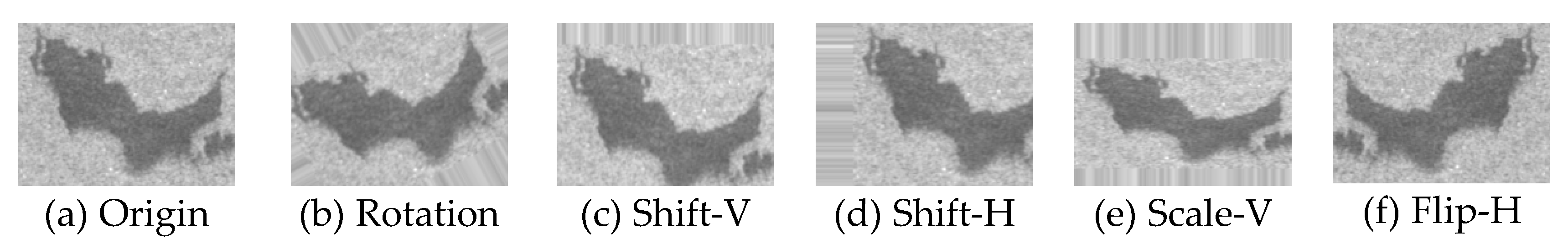
What the training of DCNN actually does is adjust thousands of weights based on the training data set and labels. In order to make all weights reach the optimal state as much as possible, the number of samples in the training data set should match the number of network parameters [33]. Data augmentation is a technique used to improve the generalization ability of the network by increasing the number of samples in the training set [34]. The noise induced by data augmentation also makes the network more robust. Data augmentation has been widely used in the training process of common DL classifiers [29,30,31]. Moreover, this method is also applied in [25,26]. Twelve operations of data augmentation are used in our case to expand the training data set. The operations include Rotation (7°, 17°, 27°, 37°, and 47°), Shift(horizontal, H; vertical, V), Scale(H, V) and Flip (H, V, HV), Examples of a typical dark patch sample with data augmentation are shown in Figure 3. The number of our training set (13,722) was expanded to the order of 105-106 with data augmentation. The training was done in the network with the original and expanded data set after the proposed network was obtained, respectively, to validate the positive effect of data augmentation (see Section 5.4 for details).
3. Determine the Basic Architecture of DCNNs
As shown in Figure 1, we firstly decided on a basic architecture, which was selected from AlexNet, VGG-16, and VGG-19 by transfer learning with our oil spill data set. Here, transfer learning [35] refers to fine tuning of the model parameters with the dark patch data set based on a model which has already been well trained with the public data set, so as to quickly achieve a good classification performance for our data set. Transfer learning requires an application domain similar to the original one, but allows it to be a little different [36].
Pre-trained models for the three networks can be downloaded from the Tensorflow group of Google on GitHub—an open source code hosting platform [37]. These pre-trained models contain the network structures and all parameters and weights trained with public RGB data sets. Transfer learning can actually be considered a special weight initialization method. In our experiments, the SAR image was a one-channel gray image instead of a three-channel RGB image; dark patch images were re-sampled to 64 × 64 on-the-fly before being fed to the network; and only two categories—oil spill and lookalike—were focused on. Therefore, what we needed to do based on these downloaded pre-trained models was to simply set their input image color channel number to 1, input image size to 64 × 64, and output category to 2, and then train further.
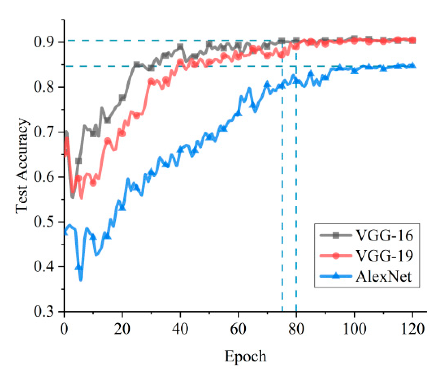
Transfer learning, as a fine-tuning technique, will not stop the training until the model test accuracy is stable. It gives us the opportunity to check how many epochs the network takes to reach a stable status. The training efficiency and classification accuracy obtained by the transfer learning of the three networks—AlexNet, VGG-16, and VGG-19—are shown in Figure 4. Obviously, the classification performance of VGG-16 and VGG-19 is better than that of AlexNet. VGG-16 and VGG-19 have almost the same classification performance, but the latter converges slower than the former, which implies that the additional three layers of VGG-19 compared to VGG-16 do not improve the classification performance, but reduce the training efficiency. Therefore, VGG-16 was used as the basic structure for further optimization in this study.
4. The Proposed DCNN for SAR Oil Spill Detection
In this section, based on the results of Section 3, the network hierarchy is designed, which includes the architecture of convolutional layers and Fully Connected layers (FCs). Then, the network hyperparameters are adjusted so that they are suitable for classifying SAR dark patches. This involves many comparative experiments using the data sets described in Section 2 with data augmentation. In these experiments, the training will be started from scratch instead of using a pre-trained model, since most attributes and hyperparameters, as well as network architecture, will be changed. These comparative experiments only need coarse tuning, which uses a relatively small number of epochs because its goal is to obtain the best value of hyperparameters instead of a well-trained network.
To use the control variable method to further determine attributes and hyperparameters, some initial conditions are employed, as follows: (1) the activation function is ReLU, (2) the loss function is softmax cross entropy, (3) dropout is 0.5, (4) the learning rate is 1e-4, (5) the batch size is 64, (6) weights are initialized in a standard normal distribution, and (7) the optimizer is Stochastic Gradient Descent (SGD) with momentum.
4.1. Structure of Convolutional Layers
According to the previous analysis, the size of input dark patches is 64 × 64, which is smaller than 224 × 224—the input size of VGG-16 based on ImageNet. This difference implies that the new network should be simpler than VGG-16 in terms of receptive fields. For a CNN, a Feature Map (FM) is produced from an input image by applying a convolution kernel. The size of an FM can be expressed as follows [38]:
where , , and are the size of the FM, input image, and convolution kernel, respectively; is the stride; and is the padding value.
The region of the original image where one pixel of an FM is mapped is called the receptive field (RF) [39]. The size of the receptive field in the first layer is equal to the size of the convolution kernel. Then, the size of the deeper layer receptive field can be iteratively calculated as follows:
where is the receptive field size of the k-th layer, is the receptive field size of the (k − 1)-th layer, and is the stride size of the i-th layer.
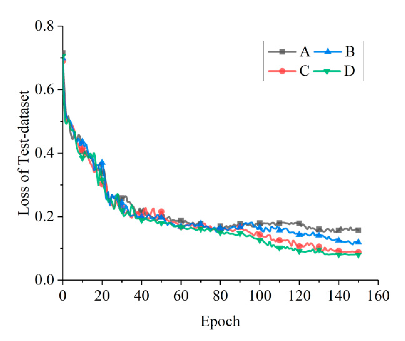
When the receptive field of the final layer is closer to, but no larger than, the image region, it is easier for convolution to obtain more information, so as to achieve a better capability of feature extraction [40]. This means that the new network should be designed so that the receptive field size of the final layer is close to 64 × 64. Shown in Table 2 is the size of the FM and RF for each layer in VGG-16, calculated by Formulas (1) and (2). is located between the layers of Stack3 and Stack4. Therefore, as shown in Table 3, four candidate networks named A, B, C, and D were designed, which include layers deep to Stack3 or Stack4. Network A is an intercept structure of VGG-16 from Stack1 to Stack3, and network B is an intercept structure of VGG-16 from Stack1 to Stack4. Network C and network D use the same structure as network A and network B, respectively, but the number of weight layers in Stack1 is reduced to one. This reduction means that more fine-grained features are obtained by the first pooling layer, thereby improving the ability of the entire network to extract detailed features [41]. The convolution layers (with different depths in different configurations) are followed by three FCs.
Similar to VGG, both the first and second FC have the same channel number, 1024; the third FC contains only two nodes for the classes of oil spill and lookalike. The configuration of the FCs is the same in networks A, B, C, and D. All of the pooling layers (Pool1, Pool2, and Pool3) in the network use the maximum pooling process, and the Rectified Linear Unit (ReLU) [29] is set as the activation function. The loss curves of the test data set obtained by training the four networks are shown in Figure 5. The losses of C and D converge significantly faster and reach lower values than those of A and B. Both the losses of C and D tend to have the same value, but C converges faster than D. According to Table 3, the structure of network C is simpler than that of D, which indicates that there is still structural redundancy in network D. Therefore, network C is the one which is most suitable for the oil spill detection data set among the four candidate networks.
4.2. Node Number of FC and Dropout
The number of nodes in one FC layer and dropout rate [42] jointly determine the number of nodes that are actually effective during training in that layer. Therefore, they should be considered together.
The number of nodes in the first FC layer of OSCNet is equivalent to the number of input features in a traditional ANN. According to the experience of AAMLP [14], that network achieved satisfactory classification results when using 77 features. This experience provides a clue for finding suitable values for the node number and dropout rate. In this section, we explore the effect of varying the hyperparameter. The comparison was conducted in two situations.
Firstly, the dropout rate was set to a common value of 0.5 [29], and the network was then trained four times with four different numbers of FC: 1024, 512, 256, and 128. The training accuracy corresponding to the four FC node numbers is shown in Table 4. The experimental results show that the classification accuracy is relatively high when the number of remaining nodes of FC is 64 or 128, which is close to the empirical value of 77.
Then, such combinations of FC node number and dropout rate (see Table 5) where the reserved node numbers of FC were between 64 and 128 were adopted to train the network. The results show (see Figure 6) that combination D has the fastest convergence speed. It is not difficult to see from Figure 6 that excessive dropouts make network training more difficult, and it is easier to obtain better results by moderate dropout. In subsequent tuning experiments for other hyperparameters, the network was initialized with combination D, i.e., the FC node number of 128 and dropout rate of 0.1.
4.3. Hyperparameter Evaluation
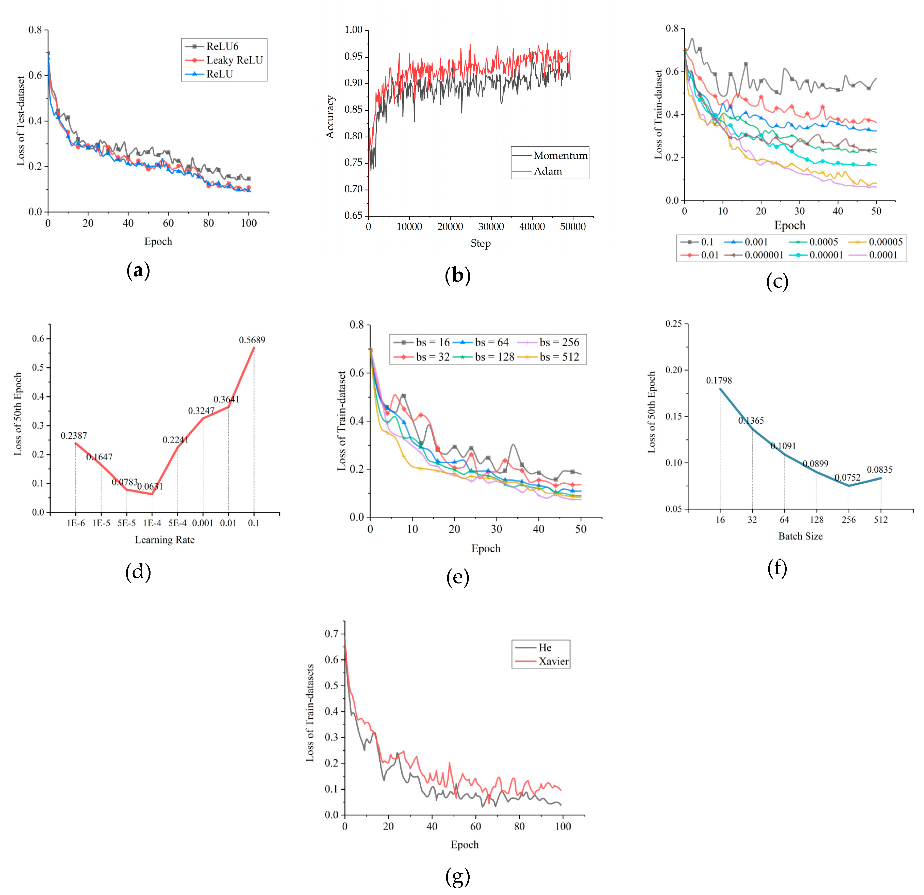
Common activation functions include Sigmoid, tanh, ReLU, and the variants of ReLU, such as Leaky ReLU and ReLU6 [43]. ReLU can avoid the problems of gradient disappearance or gradient explosion, which often happens when Sigmoid or tanh is used in deep networks [29]. Since ReLU has been widely used in AlexNet, VGG, and other networks, and has been proven to have a good universal adaptability [29,31], we only examined the sensitivity of ReLU and its variants using our data set. As shown in Figure 7a, Leaky ReLU and ReLU fit almost equally. However, compared to ReLU, when adding negative nodes to the operation, Leaky ReLU causes the network to have a greater time and space complexity, which leads to slower convergence. Therefore, we chose ReLU as the activation function. This is different from the case where Leaky ReLU is often better than ReLU in the classification problem of RGB images.
The scale of our training set was in the order of 105-106, so the training optimization algorithm used Stochastic Gradient Descent (SGD) [44]. Increasing the momentum in SGD (Momentum) can improve the efficiency of gradient descent and avoid position vibration near the minimum value of the gradient [45]. This is a popular method that has been adopted by AlexNet, VGG, and other classical CNNs. Meanwhile, Kingma et al. [46] pointed out that their adaptive moment estimation (Adam) had a better performance than Momentum. Based on SGD, the Momentum and Adam algorithms were used for multiple training. As shown in Figure 7b, Adam is better than Momentum for the SAR dark patch data set.
According to the method used to determine the initial learning rate proposed by Nielsen [47], the search direction for the optimal initial learning rate can be determined to be downward by training at the initial rates of 0.001, 0.01, and 0.1. Therefore, many smaller initial learning rates were subsequently checked. Their corresponding learning curves are shown in Figure 7c,d. According to Figure 7c,d, the initial learning rate of 5.0 × 10⁻⁵ is best for OSCNet.
Bengio et al. [48] believed that the batch size could range from one to several hundred, and values over 10 could make full use of the acceleration advantage of matrix–matrix products over matrix–vector products, thereby improving the training efficiency. Considering the hardware conditions, a comparative experiment was performed with a batch size that was increased from 16 to 512 by iterative multiples of 2, shown in Figure 7e,f. Considering the consumption of computing time, 256 was selected as the batch size for training.
The initialization of weights and biases (parameter initialization) has a significant impact on whether the network can converge, the speed of convergence, and whether it is easy to fall into a local minimum. Glorot et al. [49] designed an initialization method, known as Xavier Initialization, to ensure that the output variance of each layer is equal. In 2015, considering the influence of the non-linear effect of the ReLU series activation functions on the distribution of output data, He et al. [43] proposed an initialization method that can more likely guarantee the consistency of input and output variances of the network. The comparison experiment was conducted by training our network with the two initialization methods. The comparison result in Figure 7g shows that He initialization is better than Xavier initialization for OSCNet.
5. Experimental Results and Analysis
After completing all of the above experiments, the structure of OSCNet (see Figure 8) and the hyperparameters of the network (see Table 6) were finally determined. In order to verify the fitting and generalization capabilities of OSCNet, we preprocessed the data set 15 times, completed 15 training experiments on different training data sets, and obtained their test results, respectively.
5.1. Evaluation Metrics
Before validating 15 models, we needed to clarify the models’ validation criteria, that is, the performance indicators of common classifiers, as the validation indicators of OSCNet. These indicators include the recognition rate (accuracy), detection rate (recall), precision, F-measure, receiver operating characteristic (ROC) curve, and area under the curve (AUC). The confusion matrix of the detection results is shown in Table 7. The four values in the confusion matrix are true positives (TPs), true negatives (TNs), false positives (FPs), and false negatives (FNs).
The indicators can be defined as follows:
5.2. Results
The results of the 15 training set are shown in Table 8. The highest recognition rate (accuracy) is 95.46%, the highest detection rate (recall) is 85.17%, the best precision is 87.30%, and the best F-measure is 85.55%. The corresponding averaged values are 94.01%, 83.51%, 85.70%, and 84.59%, respectively.
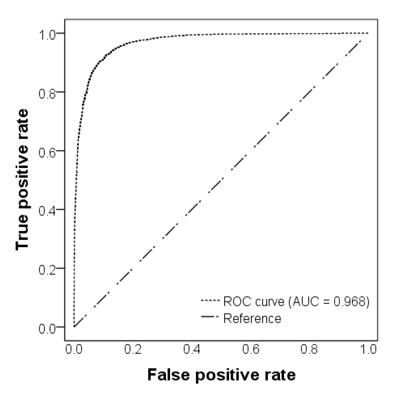
By averaging the 15 results of validation, the ROC curve and the corresponding AUC were produced and are shown in Figure 9. The ROC curve is very close to the X- and Y-axes, and the value of AUC is 0.968, which is significantly higher than 0.868—the value of AAMLP obtained in [14]. Therefore, we may say that OSCNet is better than AAMLP.
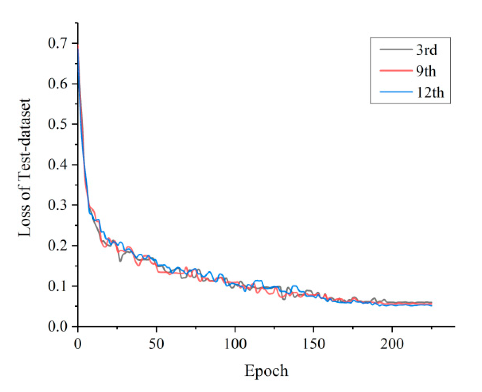
It is also important to investigate whether the performance of models is stable for the different training sets since, every time, the training set was randomly generated from the original data set. We plotted the changes in the values of loss based on the test data set: 3rd Training Model (a randomly selected training set), 9th Training Model (the detection rate is the largest), and 12th Training Model (the recognition rate is the largest). The curves are shown in Figure 10. Except for some slight random oscillations, the three curves almost coincide. This shows that the network is quite stable.
5.3. Comparison Based on the Same Data Set
The classification performances of OSCNet, VGG-16, and AAMLP obtained based on the same data set are listed in Table 9. Although OSCNet is a variant of VGG-16, it displays a better performance than that of VGG-16 by transfer learning. Compared with AAMLP, all classification performance indicators of OSCNet are improved to some degree.
We selected three typical SAR images containing oil spills to intuitively show improvement of the classification results of AAMLP by OSCNet. In the following analysis, oil spills and lookalikes are labeled 1 and 0, respectively.
The first SAR image was Envisat ASAR, acquired in the northwestern region of the Bohai Sea, China, on February 15, 2004, at 02:23:03 UTC. The variability of the image intensity with the angle of incidence was corrected. Oil spills detected by AAMLP and OSCNet are marked with boxes in Figure 11a,b, respectively. The arc-shaped dark stripes ranked from left to right on the left side of the image are the atmospheric internal waves. One of them was misclassified as an oil spill by AAMLP (see the magenta box in Figure 11a), but correctly judged as a lookalike by OSCNet. It is worth noting that there were multiple dark patches in the atmospheric internal waves, but only one of them was misclassified as an oil spill by AAMLP, which indicates that the feature vector of the atmospheric internal waves is close to the decision surface of AAMLP. Table 10 shows the classification results and accuracy of OSCNet.
The second SAR image was Envisat ASAR, acquired offshore Shanghai in the East China Sea on November 5, 2003, at 13:42:17 UTC. The oil spills detected by AAMLP and OSCNet are marked with boxes in Figure 12a,b, respectively. AAMLP reported one false alarm and missed one oil spill. The false alarm was a shoal in the estuary of Yangtze River, which appeared as a black ring on the SAR image (see number 01 in Table 11). The missed dark patch was an oil spill with a small contrast to the ocean background (see number 02 in Table 11). Both dark patches were correctly classified by OSCNet, and their confidence was greater than 0.8.
The third SAR image was acquired by COSMO-SkyMed in the east of Bohai Sea, China, on August 24, 2011, at 10:33:31 UTC. Figure 13a,b shows the respective detection results of AAMLP and OSCNet. The complex dark pattern shown on the left of the SAR image is the typical feature of a low wind speed zone in an SAR image. There were two false alarms reported by AAMLP in the low wind speed zone, while both of them were correctly classified by OSCNet with a confidence value greater than 99% (see numbers 04 and 05 in Table 12).
Although OSCNet achieved a better classification performance than AAMLP, there were still some misclassified cases, as shown in Table 13. In such cases, the classification confidence of OSCNet was usually relatively low. It must be acknowledged that there was still considerable uncertainty in the separation of dark patches by OSCNet. In fact, there was a mixed zone in the feature space for oil spills and lookalikes. For example, the SAR image features of biological oil films were very similar to those of oil spills. Without other auxiliary information, such as the environmental information and near synchronous optical remote sensing images, even experts cannot make a clear judgment on the samples in the mixed zone of a feature space. Even if the manual labels based on the auxiliary information are accurate, it is still difficult for the classifier to distinguish these dark patches based only on the information extracted from SAR images. This is the root cause of difficulties of SAR oil spill detection. In order to improve the classification performance further, it is necessary to improve the accuracy of the labels and to increase the number of samples, or import additional information into the classifier. This information may include a wider range of images around the dark patch, a synchronous wind field, or synchronous optical remote sensing images.
5.4. The Role of Data Augmentation
We previously used data augmentation to increase the size of the training set. Once the network architecture and hyperparameters of OSCNet had been fixed, we had a chance to verify the role of data augmentation in network training through experiments. The red and black curves in Figure 14 are the loss curves when training with and without data augmentation, respectively.
According to Figure 14, the loss curve of training with data augmentation converges to a lower value than that without data augmentation. At the beginning of training, the descent speed of the black curve is significantly higher than the descent speed of the red curve, but the descent stops at 0.24 and starts to oscillate upward after 120 Epoch. This shows that the network trained without data augmentation finally becomes over-fitted. This phenomenon has been explained and discussed by many researchers [29,30,31,33]. Therefore, it is necessary to train with data augmentation, which can effectively avoid over-fitting and improve the classification accuracy.
5.5. Comparison of Auto-Extracted Features and Hand-Crafted Features
A DCNN can be divided into a convolutional part and an FC part. The FC part is equivalent to a traditional neural network, and the convolutional part is responsible for automatically extracting features from the training sample set. Since the feature set used by the DCNN is what is learned by the convolutional network part from the training sample set, it is more in line with the characteristics of the data than the hand-crafted feature set which is adopted in traditional ML networks, and thus the DCNN is able, in principal, to obtain a better classification performance than that of traditional ML networks. This is supported by the following analysis.
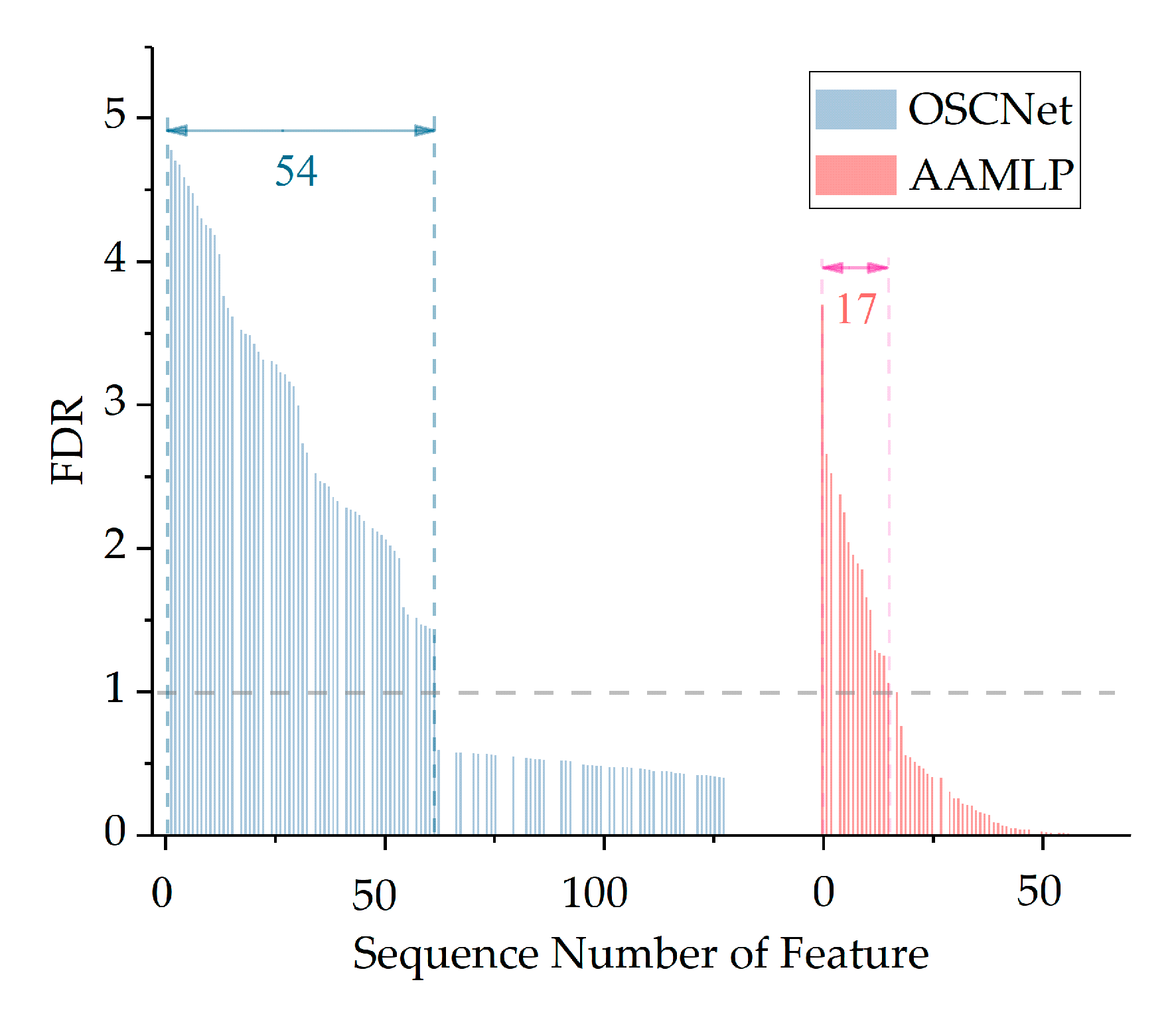
The number of nodes in the first layer of OSCNet’s FCs is 128, which indicates that there are 128 features automatically extracted by the convolutional part of the network. AAMLP has 77 artificially-defined features, which are collected from a large number of papers or books related to automatic SAR oil spill detection or image pattern recognition. For each feature, the mean and standard deviation can be calculated for the oil spills and the lookalikes, respectively. The Fisher’s Discriminant Ratio (FDR) [50] for each feature can then be calculated using Formula (7), which describes the capability of a single feature to distinguish the two classes of oil spill and lookalike.
The larger the FDR value is, the higher the capability of discrimination is [50].
Figure 15 shows the FDRs for all features used by OSCNet and AAMLP. The blue part on the left is OSCNet and the red part on the right is AAMLP. Since we did not care about the physical meaning of the features, they just needed to be numbered. The abscissa in the figure is the feature number, and the features are arranged in descending order of FDR for OSCNet and AAMLP, respectively.
In addition, the correlation coefficients were calculated for all the features in the same feature set in pairs, and the features with a correlation coefficient greater than 95% were regarded as similar features. In this way, one feature set could be divided into many similar feature groups. Only the feature with the highest FDR was retained in each group and the other similar features were deleted, so many gaps are left in Figure 15. We considered these retained features as valid features.
It can be seen from Figure 15 that the overall FDR values of the features of OSCNet are significantly higher than those of AAMLP. The number of valid features with FDR > 1 in OSCNet is 54, while the number in AAMLP is only 17. Therefore, the distinguishability of the features automatically learned by OSCNet is significantly higher than the hand-crafted features used in AAMLP, which is an important reason for the higher classification performance of OSCNet than AAMLP.
5.6. Comparison with Other DL Classifiers
In this section, the comparison of OSCNet with several DL classifiers for SAR oil spill detection, including GCNN [24], TSCNN [25], and RED-Net [26], will be presented in terms of the network depth, data set size, data source, and classification performance indicators. Since OSCNet works at the dark patch level, but TSCNN and REDNet work at the pixel level, we also calculated a set of pixel-based classification performance indicators for OSCNet (see Table 14). The formulas employed for generating the classification performance indicators are the same as the formulas (3)-(6), except for the fact that the values of the confusion matrix are pixel numbers instead of dark patch numbers. The indicators calculated by the pixel number are usually different from those calculated by the dark patch number because dark patch sizes in the data set are variable.
Using the averaged (AVG) value, we compared OSCNet with TSCNN and REDNet based on pixel-based classification performance indicators (see Table 15).
A remarkable feature in Table 15 is that the numbers of samples, SAR images, and SAR data sources used by OSCNet are much larger than those of other works. To some degree, the size of the data set determines the validity of statistic characteristics and whether the source of the data set is widespread may affect the generalization of the network for various types of data. Both TSCNN and RED-Net use smaller data sets and contain only one data source. The data source of GCNN is also singular. In this sense, the indicators given by OSCNet should have a relatively strong generalization ability in the problem domain of spaceborne SAR oil spill detection.
Another remarkable feature in Table 15 is that OSCNet is much deeper than the other networks. This is mainly due to the larger size of our data set and data augmentation. According to the study of Lei et al. [33], the minimum data set size required when the network is close to optimal is related to the number of weights of the network. Their experiments showed that a network with 1.14 × 10⁶ weights needs the size of the training data set to be at least about 4 × 10⁴. Following the proportion, the size of the data set required by OSCNet might be greater than 9.5 × 10⁴. After data augmentation, the training set size of OSCNet expanded to 1.6 × 10⁵, which meets the above requirements.
Concerning the classification performance indicators, because the data sets of OSCNet and the other three classifiers are very different, it makes almost no sense to compare them directly. The indicators can only be references of the classifiers in their own problem domains. In spite of the different problem domains, the most outstanding performance is achieved by RED-Net, followed by OSCNet. RED-Net’s precision, recall, and F-measure are all much higher than those of OSCNet. However, we notice that the input size of the RED-Net is determined by its data set through the grid search algorithm, while the size of the dark patches in our data set varies in an extremely wide range. As mentioned in Section 2.2, the size of an oil spill dark patch can be as large as 2136. Therefore, it is doubtful whether similar excellent indicators can be achieved by RED-Net based on our data set with such a wide ranging dark patch size, even if a new input size is determined by the grid search method. Nevertheless, this method based on image segmentation to solve oil spill detection in one step is worth learning from. Considering the heavy workload, we will carry out related experiments in future research.
6. Conclusions and Outlooks
Based on VGG-16, a relatively deep DCNN named OSCNet was built in this study for the classification of SAR dark patches. OSCNet contains as many as 12 weight layers, which benefits from the use of the data augmentation technique for the big data set composed of 23,768 SAR dark patches extracted from 336 SAR images. The distinguishability of the features learned from the data set by OSCNet is much better than that of hand-craft features. Therefore, the classification performance of OSCNet is significantly improved compared to AAMLP—a traditional sophisticated ML classifier. The accuracy, recall, and precision were increased from 92.50%, 81.40%, and 80.95% to 94.01%, 83.51% and 85.70%, respectively. The classification performance of OSCNet might be better than that of the other two CNN-type networks [24,25], which are currently available for SAR oil spill detection, but probably not as good as RED-Net [26]—a pixel-level DL classifier.
Our research shows that the size and statistic characteristic of the data set play a crucial role in the establishment of a DCNN classifier for SAR oil spill detection. In order to build an automatic operational SAR oil spill monitoring system, continuously expanding the data set should be a long-standing task.
For a system based on the three-step processing framework, the procedure used to automatically extract dark patches from SAR images must always be consistent, because the statistical characteristics of the dark patch data set are also affected by the image segmentation program. This effect is mainly reflected in the proportion of lookalikes. The dark patches in this research were all extracted by the same image segmentation program and thus meet the above requirements.
The pixel-level classifier can be used as an image segmentation algorithm in a three-step processing framework if its recall is 100%, at the expense of precision. However, if acceptable values can be obtained for both recall and precision simultaneously, the pixel-level classifier can exist as an independent SAR oil spill detector other than a classifier in the three-step processing framework. At this point, it will pose an important challenge to the three-step processing framework. In future research, we will pay more attention to the pixel-level DL classification algorithms and compare them with dark patch-level DL algorithms based on the same big data set so as to find the better algorithms among them for SAR oil spill detection.
Author Contributions
K.Z. and Y.W. conceived and designed the experiments; Y.W. performed the experiments; K.Z. analyzed the results; Y.W. and K.Z. wrote the original manuscript; K.Z. edited the manuscript. All authors read and approved the final manuscript.
Funding
This research was funded by CNOOC Environmental Services (Tianjin) Co., Ltd. Research Fund, Grant No. CY-HB-13-ZC-023.
Acknowledgments
The SAR images of ERS-1,2/SAR and Envisat/ASAR were provided by the European Space Agency (ESA) freely through the ESA EO data gateway under the ESA-MOST Dragon 3 Program (id 10580) and Dragon 4 Program (id 32281).
Conflicts of Interest
The authors declare no conflicts of interest.
References
- Smith, L.; Smith, M.; Ashcroft, P. Analysis of environmental and economic damages from British Petroleum’s Deepwater Horizon oil spill. Albany Law Rev. 2011, 74, 563–585. [Google Scholar] [CrossRef] [Green Version]
- Lan, G.; Li, Y.; Chen, P. Time Effectiveness Analysis of Remote Sensing Monitoring of Oil Spill Emergencies: A Case Study of Oil Spill in the Dalian Xingang Port. Adv. Mar. Sci. 2012, 4, 13. [Google Scholar]
- Yin, L.; Zhang, M.; Zhang, Y. The long-term prediction of the oil-contaminated water from the Sanchi collision in the East China Sea. Acta Oceanol. Sin. 2018, 37, 69–72. [Google Scholar] [CrossRef]
- Yu, W.; Li, J.; Shao, Y. Remote sensing techniques for oil spill monitoring in offshore oil and gas exploration and exploitation activities: Case study in Bohai Bay. Pet. Explor. Dev. 2007, 34, 378. [Google Scholar]
- Qiao, F.; Wang, G.; Yin, L.; Zeng, K.; Zhang, Y.; Zhang, M.; Xiao, B.; Jiang, S.; Chen, H.; Chen, G. Modelling oil trajectories and potentially contaminated areas from the Sanchi oil spill. Sci. Total Environ. 2019, 685, 856–866. [Google Scholar] [CrossRef]
- Keydel, W.; Alpers, W. Detection of oil films by active and passive microwave sensors. Adv. Space Res. 1987, 7, 327–333. [Google Scholar] [CrossRef]
- Uhlmann, S.; Serkan, K. Classification of dual- and single polarized SAR images by incorporating visual features. ISPRS J. Photogramm. Remote Sens. 2014, 90, 10–22. [Google Scholar] [CrossRef]
- Brekke, C.; Solberg, H. Oil spill detection by satellite remote sensing. Remote Sens. Environ. 2005, 95, 1–13. [Google Scholar] [CrossRef]
- Nirchio, F.; Sorgente, M.; Giancaspro, A. Automatic detection of oil spills from SAR images. Int. J. Remote Sens. 2005, 26, 1157–1174. [Google Scholar] [CrossRef]
- Solberg, H.; Solberg, R. A large-scale evaluation of features for automatic detection of oil spills in ERS SAR images. In Proceedings of the 1996 IEEE International Geoscience and Remote Sensing Symposium (IGARSS), Lincoln, NE, USA, 31 May 1996; Volume 3, pp. 1484–1486. [Google Scholar]
- Topouzelis, K.; Psyllos, A. Oil spill feature selection and classification using decision tree forest on SAR image data. ISPRS J. Photogramm. Remote Sens. 2012, 68, 135–143. [Google Scholar] [CrossRef]
- Singha, S.; Vespe, M.; Trieschmann, O. Automatic Synthetic Aperture Radar based oil spill detection and performance estimation via a semi-automatic operational service benchmark. Mar. Pollut. Bull. 2013, 73, 199–209. [Google Scholar] [CrossRef] [PubMed]
- Topouzelis, K.; Karathanassi, V.; Pavlakis, P. Detection and discrimination between oil spills and look-alike phenomena through neural networks. ISPRS J. Photogramm. Remote Sens. 2007, 62, 264–270. [Google Scholar] [CrossRef]
- Zeng, K. Development of Automatic Identification and Early Warning Operational System for Marine Oil Spill Satellites—Automatic Operation Monitoring System for Oil Spill from SAR Images; Technical Report; Ocean University of China: Qingdao, China, 2017. [Google Scholar]
- Del, F.; Petrocchi, A.; Lichtenegger, J. Neural networks for oil spill detection using ERS-SAR data. IEEE Trans. Geosci. Remote Sens. 2000, 38, 2282–2287. [Google Scholar]
- Stathakis, D.; Topouzelis, K.; Karathanassi, V. Large-scale feature selection using evolved neural networks. In Proceedings of the 2006 Image and Signal Processing for Remote Sensing, International Society for Optics and Phonetics, Ispra, Italy, 6 October 2006; Volume 6365, pp. 1–9. [Google Scholar]
- Singha, S.; Bellerby, T.; Trieschmann, O. Satellite oil spill detection using artificial neural networks. IEEE J. Sel. Top. Appl. Earth Obs. Remote Sens. 2013, 6, 2355–2363. [Google Scholar] [CrossRef]
- Brekke, C.; Solberg, H. Classifiers and confidence estimation for oil spill detection in ENVISAT ASAR images. IEEE Geosci. Remote Sens. Lett. 2008, 5, 65–69. [Google Scholar] [CrossRef]
- Xu, L.; Li, J.; Brenning, A. A comparative study of different classification techniques for marine oil spill identification using RADARSAT-1 imagery. Remote Sens. Environ. 2014, 141, 14–23. [Google Scholar] [CrossRef]
- Singha, S.; Ressel, R.; Velotto, D. A combination of traditional and polarimetric features for oil spill detection using TerraSAR-X. IEEE J. Sel. Top. Appl. Earth Obs. Remote Sens. 2016, 9, 4979–4990. [Google Scholar] [CrossRef] [Green Version]
- Solberg, H.; Volden, E. Incorporation of prior knowledge in automatic classification of oil spills in ERS SAR images. In Proceedings of the 1997 IEEE International Geoscience and Remote Sensing Symposium (IGARSS), Singapore, 3–8 August 1997; Volume 1, pp. 157–159. [Google Scholar]
- Solberg, H.; Storvik, G.; Solberg, R. Automatic detection of oil spills in ERS SAR images. IEEE Trans. Geosci. Remote Sens. 1999, 37, 1916–1924. [Google Scholar] [CrossRef] [Green Version]
- Huang, X.; Wang, X. The classification of synthetic aperture radar oil spill images based on the texture features and deep belief network. In Computer Engineering and Networking; Springer: Cham, Switzerland, 2014; pp. 661–669. [Google Scholar]
- Guo, H.; Wu, D.; An, J. Discrimination of oil slicks and lookalikes in polarimetric SAR images using CNN. Sensors 2017, 17, 1837. [Google Scholar] [CrossRef] [Green Version]
- Nieto-Hidalgo, M.; Gallego, A.J.; Gil, P. Two-stage convolutional neural network for ship and spill detection using SLAR images. IEEE Trans. Geosci. Remote Sens. 2018, 56, 5217–5230. [Google Scholar] [CrossRef] [Green Version]
- Gallego, A.J.; Gil, P.; Pertusa, A. Segmentation of oil spills on side-looking airborne radar imagery with autoencoders. Sensors 2018, 18, 797. [Google Scholar] [CrossRef] [PubMed] [Green Version]
- Ball, J.; Anderson, D.; Chan, C. Comprehensive survey of deep learning in remote sensing: Theories, tools, and challenges for the community. J. Appl. Remote Sens. 2017, 11. [Google Scholar] [CrossRef] [Green Version]
- LeCun, Y.; Bottou, L.; Bengio, Y. Gradient-based learning applied to document recognition. Proc. IEEE 1998, 86, 2278–2324. [Google Scholar] [CrossRef] [Green Version]
- Krizhevsky, A.; Sutskever, I.; Hinton, G.E. Imagenet classification with deep convolutional neural networks. In Advances in Neural Information Processing Systems (NIPS); NeurIPS: Vancouver, BC, Canada, 2012; pp. 1097–1105. [Google Scholar]
- Zeiler, M.D.; Fergus, R. Visualizing and understanding convolutional networks. In Proceedings of the 2014 European Conference on Computer Vision, Zurich, Switzerland, 6–12 September 2014; Volume 8689, pp. 818–833. [Google Scholar]
- Simonyan, K.; Zisserman, A. Very deep convolutional networks for large-scale image recognition. arXiv 2017, arXiv:1409.1556. [Google Scholar]
- He, K.; Zhang, X.; Ren, S.; Sun, J. Spatial pyramid pooling in deep convolutional networks for visual recognition. IEEE Trans. Pattern Anal. Mach. Intell. 2015, 37, 1904–1916. [Google Scholar] [CrossRef] [PubMed] [Green Version]
- Lei, S.; Zhang, H.; Wang, K.; Su, Z. How Training Data Affect the Accuracy and Robustness of Neural Networks for Image Classification. In Proceedings of the 2019 International Conference on Learning Representations (ICLR-2019), New Orleans, LA, USA, 6–9 May 2019. [Google Scholar]
- Perez, L.; Wang, J. The effectiveness of data augmentation in image classification using deep learning. arXiv 2017, arXiv:1712.04621. [Google Scholar]
- Pan, S.J.; Tsang, I.W.; Kwok, J.T. Domain adaptation via transfer component analysis. IEEE Trans. Neural Netw. 2010, 22, 199–210. [Google Scholar] [CrossRef] [Green Version]
- Pan, S.; Yang, Q. A Survey on Transfer Learning. IEEE Trans. Knowl. Data Eng. 2010, 22, 1345–1359. [Google Scholar] [CrossRef]
- TensorFlow image classification model library. Available online: https://github.com/tensorflow/models/tree/master/research/slim/#Pretrained (accessed on 22 January 2018).
- A Guide to Receptive Field Arithmetic for Convolutional Neural Networks. Available online: https://medium.com/mlreview/a-guide-to-receptive-field-arithmetic-for-convolutional-neural-networks-e0f514068807 (accessed on 6 April 2017).
- Canziani, A.; Paszke, A.; Culurciello, E. An analysis of deep neural network models for practical applications. arXiv 2016, arXiv:1605.07678. [Google Scholar]
- Cao, X. A Practical Theory for Designing Very Deep Convolutional Neural Networks; Technical Report; Kaggle: Melbourne, Australia, 2015. [Google Scholar]
- Mao, X.; Shen, C.; Yang, Y. Image restoration using very deep convolutional encoder-decoder networks with symmetric skip connections. In Advances in Neural Information Processing Systems (NIPS); NeurIPS: Vancouver, BC, Canada, 2016; pp. 2802–2810. [Google Scholar]
- Srivastava, N.; Hinton, G.; Krizhevsky, A. Dropout: A simple way to prevent neural networks from overfitting. J. Mach. Learn. Res. 2014, 15, 1929–1958. [Google Scholar]
- He, K.; Zhang, X.; Ren, S. Delving deep into rectifiers: Surpassing human-level performance on imagenet classification. In Proceedings of the IEEE International Conference on Computer Vision and Pattern Recognition, Boston, MA, USA, 8–10 June 2015; pp. 1026–1034. [Google Scholar]
- Ruder, S. An overview of gradient descent optimization algorithms. arXiv 2016, arXiv:1609.04747. [Google Scholar]
- Qian, N. On the momentum term in gradient descent learning algorithms. Neural Netw. 1999, 12, 145–151. [Google Scholar] [CrossRef]
- Kingma, P.; Ba, J. Adam: A method for stochastic optimization. arXiv 2014, arXiv:1412.6980. [Google Scholar]
- Nielsen, A. Neural Networks and Deep Learning; Springer: San Francisco, CA, USA, 2015. [Google Scholar]
- Bengio, Y. Practical Recommendations for Gradient-Based Training of Deep Architectures; Springer: Heidelberg/Berlin, Germany, 2012; pp. 437–478. [Google Scholar]
- Glorot, X.; Bengio, Y. Understanding the difficulty of training deep feedforward neural networks. In Proceedings of the 2010 Thirteenth International Conference on Artificial Intelligence and Statistics, Sardinia, Italy, 13–15 May 2010; Volume 9, pp. 249–256. [Google Scholar]
- Theodoridis, S.; Koutroumbas, K. Pattern Recognition, 4th ed.; Publishing House of Electronics Industry: Beijing, China, 2010; p. 660. [Google Scholar]
Figure 1.
The design flowchart of the Oil Spill Convolutional Network (OSCNet) based on candidate deep convolutional neural networks (DCNNs).
Figure 1.
The design flowchart of the Oil Spill Convolutional Network (OSCNet) based on candidate deep convolutional neural networks (DCNNs).
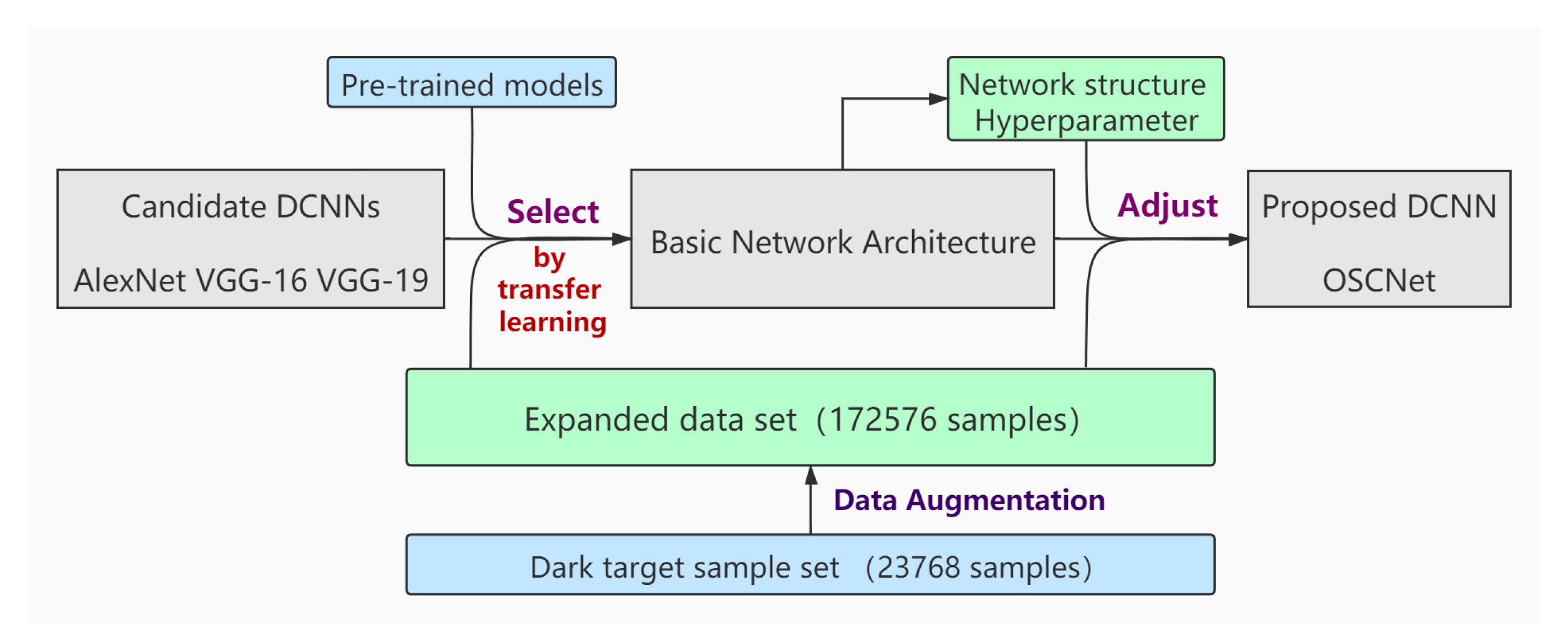
Figure 2.
The distribution of the image size of dark patch images.

Figure 3.
Examples of different data augmentation operations applied on a dark patch: (a) the original image; (b) the rotated image; (c) the vertically shifted image; (d) the horizontally shifted image; (e) the vertically scaled image; (f) the horizontally flipped image.
Figure 3.
Examples of different data augmentation operations applied on a dark patch: (a) the original image; (b) the rotated image; (c) the vertically shifted image; (d) the horizontally shifted image; (e) the vertically scaled image; (f) the horizontally flipped image.

Figure 4.
Accuracy of three general deep convolutional neural networks (DCNNs).

Figure 5.
The loss curves of four networks with different convolutional layer structures.
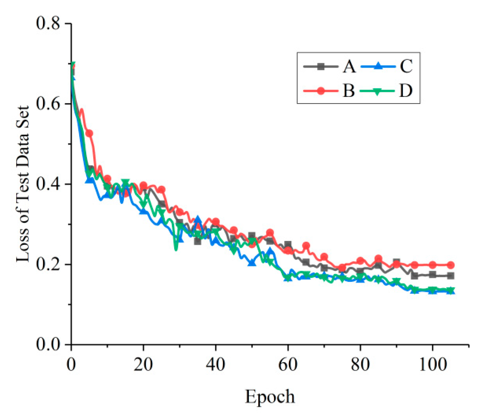
Figure 6.
Different combinations of the Fully Connected layer (FC) node number and dropout rate have different convergence speeds in the test data set.
Figure 6.
Different combinations of the Fully Connected layer (FC) node number and dropout rate have different convergence speeds in the test data set.

Figure 7.
Some curves of adjustment results in hyperparameter evaluation: (a) Different kinds of activation functions influence the decrease of loss value; (b) the two optimization algorithms achieve distinct accuracy trends; (c) the influence of the initial learning rate on the downtrend of loss; (d) loss values of the 50th Epoch in (c); (e) the influence of the batch size on the downtrend of loss; (f) loss values of the 50th Epoch in (e); (g) the influence of different initialization methods on training.

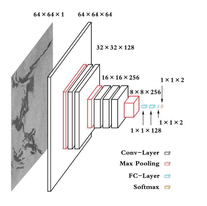
Figure 8.
The network structure of OSCNet.
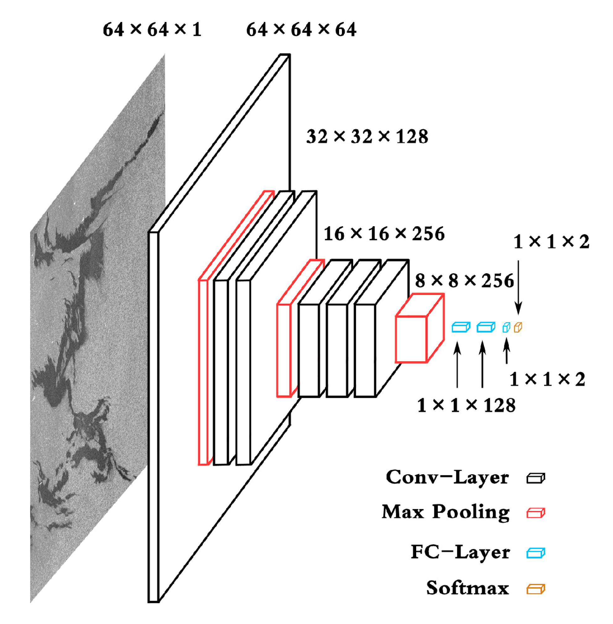
Figure 9.
Receiver operating characteristic (ROC) curve and area under the curve (AUC).

Figure 10.
Loss curves of the 3rd, 9th, and 12th training set.

Figure 11.
Typical SAR image containing oil spills: (a) Oil spills classified by the Area weighted Adaboost Multi-Layer Perceptron (AAMLP). The dark patch marked with a magenta box is a false alarm due to an atmospheric internal wave; (b) oil spills classified by OSCNet. The false alarm of (a) has been removed.
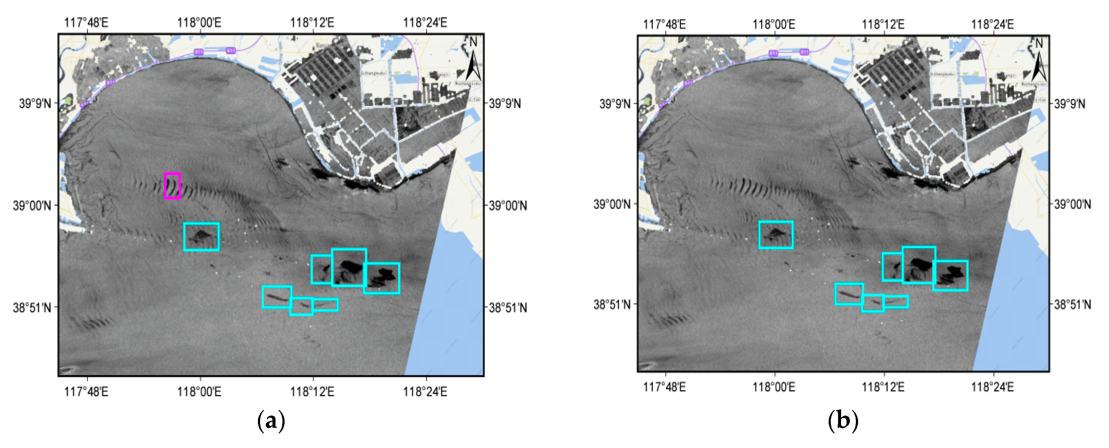
Figure 12.
Typical SAR image containing oil spills: (a) Oil spills classified by AAMLP. The dark patch marked with a magenta box is a false alarm due to shoal; (b) oil spills classified by OSCNet. The false alarm of (a) has disappeared and the dark patch marked with an orange box is missed by AAMLP, but correctly classified by OSCNet.
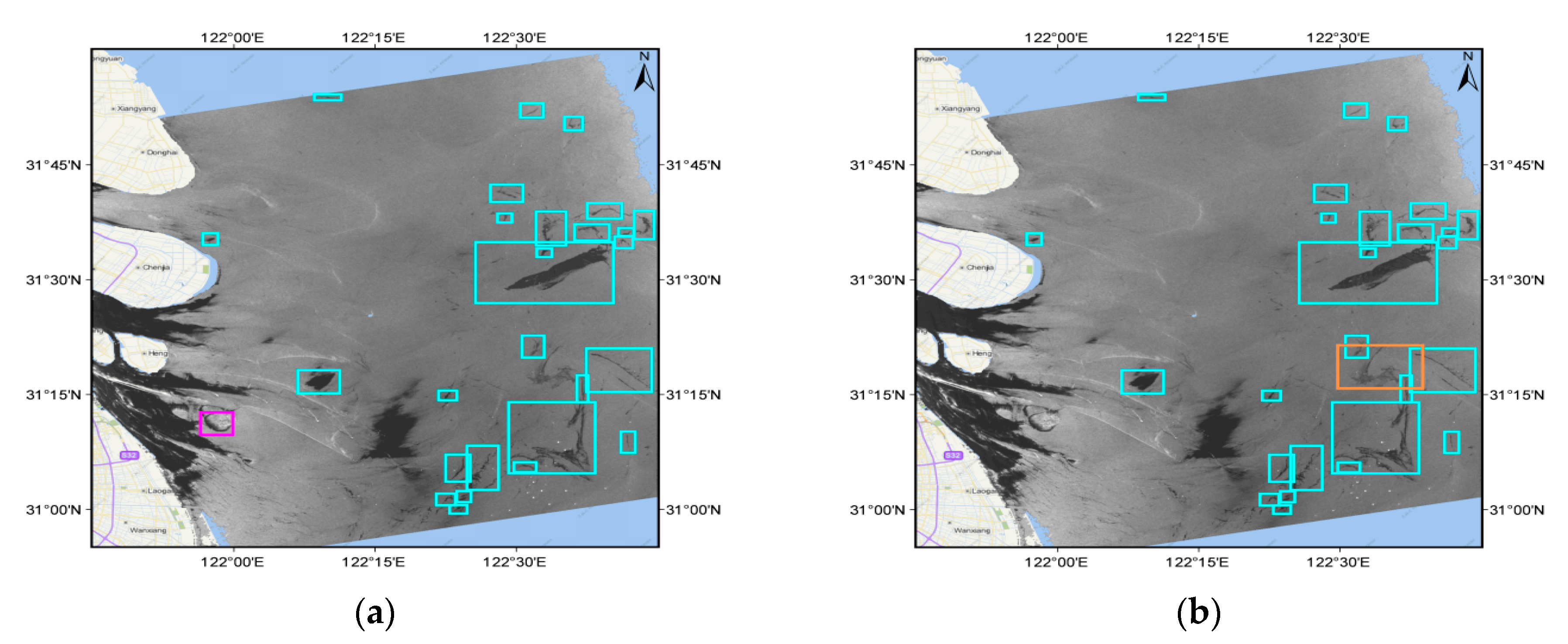
Figure 13.
Typical SAR image containing oil spills: (a) Oil spills classified by AAMLP. The dark patches marked with magenta boxes are false alarms in a low wind speed zone; (b) oil spills classified by OSCNet. The false alarms in (a) have disappeared.
Figure 13.
Typical SAR image containing oil spills: (a) Oil spills classified by AAMLP. The dark patches marked with magenta boxes are false alarms in a low wind speed zone; (b) oil spills classified by OSCNet. The false alarms in (a) have disappeared.
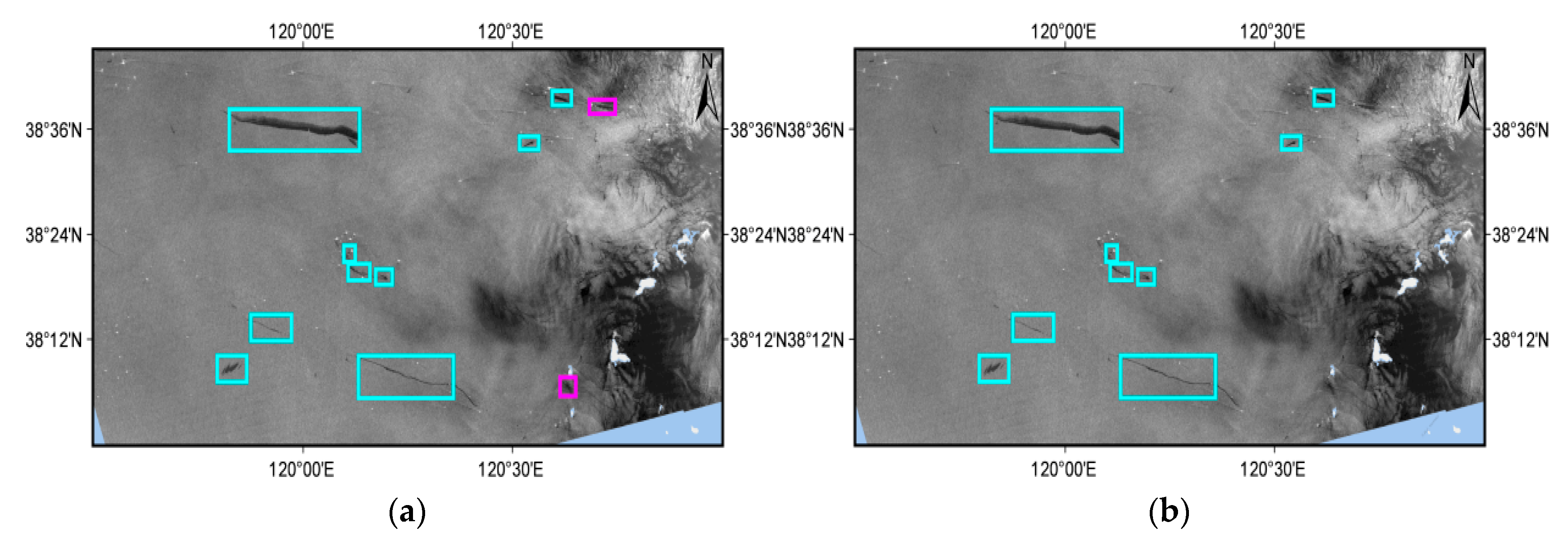
Figure 14.
The loss curves for training OSCNet with and without data augmentation.

Figure 15.
Fisher’s Discriminant Ratios (FDRs) of the features. The blue part (left) represents OSCNet and the red part (right) represents AAMLP. The gaps in the features are those removed for similar features. The number of valid features with FDR > 1 is 54 and 17 for OSCNet and AAMLP, respectively.


Table 1.
Information of original synthetic aperture radar (SAR) image sources.
| Satellite/SAR Band | Geography/Period | Number |
|---|---|---|
| Envisat/C | Bohai Sea/2011.6–2011.8 | 10 |
| China Sea/2002.11–2007.3 | 67 | |
| the Gulf of Mexico/2010.4–2010.7 | 45 | |
| European Seas, China Sea/1994.10–2009.7 | 16 | |
| ERS-1,2/C | China Sea/1992.9–2005.6 | 63 |
| COSMO Sky-Med/X | Bohai Sea/2011.6–2011.11 | 135 |
| Total | 336 |
Table 2.
Values of the feature map (FM) and receptive field (RF) in each layer of VGG-16.
| Stack | Layer | FM | RF | Stride | Stack | Layer | FM | RF | Stride |
|---|---|---|---|---|---|---|---|---|---|
| 1 | Conv3-64 | 224 | 3 | 1 | Pool3 | 28 | 44 | 8 | |
| Conv3-64 | 224 | 5 | 1 | 4 | Conv3-512 | 28 | 60 | 8 | |
| Pool1 | 112 | 6 | 2 | Conv3-512 | 28 | 76 | 8 | ||
| 2 | Conv3-128 | 112 | 10 | 2 | Conv3-512 | 28 | 92 | 8 | |
| Conv3-128 | 112 | 14 | 2 | Pool4 | 14 | 100 | 16 | ||
| Pool2 | 56 | 16 | 4 | 5 | Conv3-512 | 14 | 132 | 16 | |
| 3 | Conv3-256 | 56 | 24 | 4 | Conv3-512 | 14 | 164 | 16 | |
| Conv3-256 | 56 | 32 | 4 | Conv3-512 | 14 | 196 | 16 | ||
| Conv3-256 | 56 | 40 | 4 | Pool5 | 7 | 212 | 32 |
Table 3.
Network structures of the four networks.
| Stack | A | B | C | D |
|---|---|---|---|---|
| 10 weight layers | 13 weight layers | 9 weight layers | 12 weight layers | |
| Input (64 × 64 SAR image) | ||||
| 1 | conv3-64 conv3-64 | conv3-64 conv3-64 | conv3-64 | conv3-64 |
| maxpool/2 | ||||
| 2 | conv3-128 conv3-128 | conv3-128 conv3-128 | conv3-128 conv3-128 | conv3-128 conv3-128 |
| maxpool/2 | ||||
| 3 | conv3-256 conv3-256 conv3-256 | conv3-256 conv3-256 conv3-256 | conv3-256 conv3-256 conv3-256 | conv3-256 conv3-256 conv3-256 |
| maxpool/2 | ||||
| 4 | / | conv3-512 conv3-512 conv3-512 | / | conv3-512 conv3-512 conv3-512 |
| / | maxpool/2 | / | maxpool/2 | |
| FC-1024 | ||||
| FC-1024 | ||||
| FC-2 | ||||
| Softmax | ||||
Table 4.
Accuracy of the training data set from four different models.
| FC Node Num | Reserved Node Num | Training Accuracy (%) |
|---|---|---|
| 1024 | 512 | 93.95 |
| 512 | 256 | 94.75 |
| 256 | 128 | 97.08 |
| 128 | 64 | 96.88 |
Table 5.
Variable combination of the channel number and dropout rate.
| Model | FC Channel Num | Dropout Rate | Reserved Num |
|---|---|---|---|
| A | 512 | 0.8 | 102 |
| B | 256 | 0.6 | 102 |
| C | 256 | 0.5 | 128 |
| D | 128 | 0.1 | 115 |
Table 6.
Attributes and hyperparameters of OSCNet.
| Type | Activation Function | Loss Function | Dropout Rate | Learning Rate | Batch Size | Parameter Initialization |
|---|---|---|---|---|---|---|
| Method/Value | ReLU | Softmax Cross Entropy | 0.1 | 5 × 10⁻⁵ | 256 | He Initialization |
Table 7.
Confusion Matrix.
| Label | |||
|---|---|---|---|
| Oil spills | Lookalikes | ||
| Classification | Oil spills | TP | FP |
| Lookalikes | FN | TN | |
Table 8.
Classification indicators.
| Training Times | Recognition Rate | Detection Rate | Precision | F-Measure |
|---|---|---|---|---|
| 1 | 93.41 | 82.33 | 84.34 | 83.32 |
| 2 | 93.77 | 83.50 | 85.07 | 84.28 |
| 3 | 93.94 | 82.31 | 86.68 | 84.45 |
| 4 | 94.14 | 84.92 | 85.67 | 85.29 |
| 5 | 94.11 | 82.57 | 87.30 | 84.87 |
| 6 | 93.91 | 83.45 | 85.71 | 84.56 |
| 7 | 94.03 | 83.85 | 85.85 | 84.83 |
| 8 | 93.86 | 83.41 | 85.53 | 84.45 |
| 9 | 94.25 | 85.17 | 85.95 | 85.55 |
| 10 | 94.07 | 83.76 | 86.22 | 84.96 |
| 11 | 94.11 | 84.72 | 86.36 | 85.53 |
| 12 | 95.46 | 83.74 | 86.05 | 84.88 |
| 13 | 93.57 | 83.11 | 84.51 | 83.80 |
| 14 | 93.28 | 82.95 | 83.37 | 83.16 |
| 15 | 94.12 | 82.84 | 87.07 | 84.91 |
| AVG | 94.01 | 83.51 | 85.70 | 84.59 |
Table 9.
Performance comparison of different classifiers.
| Classifiers | OSCNet | VGG-16 | AAMLP |
|---|---|---|---|
| Recognition rate (accuracy) | 94.01 | 90.35 | 92.50 |
| Detection rate (recall) | 83.51 | 77.63 | 81.40 |
| Precision | 85.70 | 75.01 | 80.95 |
| F-measure | 84.59 | 76.30 | 81.28 |
Table 10.
Classification results of OSCNet.
| Sample |  |  |  |  |  |  |  |  |
| Number | 01 | 02 | 03 | 04 | 05 | 06 | 07 | 08 |
| Classification | 0 | 1 | 1 | 1 | 1 | 1 | 1 | 1 |
| Accuracy | 0.7461 | 0.9978 | ~1.0 | 0.9994 | 0.9509 | 0.9988 | 0.9987 | 0.9169 |
Table 11.
The dark patches misclassified by AAMLP, but correctly classified by OSCNet.
| Sample |  |  |
| Number | 01 | 02 |
| Classification | 0 | 1 |
| Accuracy | 0.8109 | 0.8098 |
Table 12.
Some dark patches correctly classified by OSCNet.
| Sample |  |  |  |  |  |
| Number | 01 | 02 | 03 | 04 | 05 |
| Classification | 1 | 1 | 1 | 0 | 0 |
| Accuracy | 0.9985 | 0.8705 | 0.9834 | 0.9999 | 0.9964 |
Table 13.
Examples of lookalikes hard to classify.
| Sample |  |  |  |  |  |  |
| Label | 0 | 0 | 0 | 0 | 0 | 0 |
| Classification | 1 | 1 | 1 | 1 | 1 | 1 |
| Accuracy | 0.5354 | 0.5299 | 0.5877 | 0.5763 | 0.5622 | 0.5779 |
| Sample |  |  |  |  |  |  |
| Label | 0 | 0 | 0 | 0 | 0 | 0 |
| Classification | 0 | 0 | 0 | 0 | 0 | 0 |
| Accuracy | 0.5229 | 0.5494 | 0.5790 | 0.5777 | 0.5683 | 0.5304 |
Table 14.
Pixel-level classification performance indicators of OSCNet.
| Training Times | Accuracy (%) | Recall (%) | Precision (%) | F-Measure(%) |
|---|---|---|---|---|
| 1 | 90.23 | 85.96 | 64.54 | 73.72 |
| 2 | 94.39 | 84.91 | 76.75 | 80.63 |
| 3 | 96.35 | 88.99 | 88.69 | 88.83 |
| 4 | 95.85 | 79.70 | 82.59 | 81.12 |
| 5 | 96.70 | 89.19 | 77.57 | 82.97 |
| 6 | 93.29 | 77.35 | 90.07 | 83.23 |
| 7 | 94.12 | 76.86 | 79.01 | 77.92 |
| 8 | 94.04 | 69.80 | 85.62 | 76.90 |
| 9 | 95.90 | 84.59 | 96.39 | 90.11 |
| 10 | 96.67 | 86.94 | 95.49 | 91.01 |
| 11 | 96.64 | 89.08 | 88.47 | 88.78 |
| 12 | 95.87 | 91.58 | 88.03 | 89.77 |
| 13 | 96.90 | 93.36 | 86.90 | 90.02 |
| 14 | 92.91 | 67.38 | 78.35 | 72.45 |
| 15 | 96.60 | 96.71 | 80.98 | 88.15 |
| AVG | 95.09 | 84.30 | 84.12 | 84.21 |
Table 15.
Comparison of OSCNet and existing related work.
| Classifiers | OSCNet | GCNN | TSCNN | RED-Net | |
|---|---|---|---|---|---|
| Depth of layers | 12 | 5 | 6 | 6 | |
| Data set size | 23,768 | 5400 | - | - | |
| With augmentation | Yes | No | Yes | Yes | |
| Raw SAR images | 336 | 5 | 23 | 38 | |
| Oil spills | 4843 | 1800 | 14 | 22 | |
| Data sources (Satellite/SAR band) | Envisat/C ERS-1,2/C COSMO Sky-Med/X | Radarsat-2/C | SLAR | SLAR | |
| By dark patches | Recognition rate | 94.01 | 91.33 | - | - |
| Detection rate | 83.51 | - | - | - | |
| False alarm rate | 3.42 | - | - | - | |
| By pixels | Accuracy | 95.09 | - | 97.82 | - |
| Precision | 84.12 | - | 52.23 | 93.12 | |
| Recall | 84.29 | - | 72.70 | 92.92 | |
| F-measure | 84.21 | - | 53.62 | 93.01 |
© 2020 by the authors. Licensee MDPI, Basel, Switzerland. This article is an open access article distributed under the terms and conditions of the Creative Commons Attribution (CC BY) license (http://creativecommons.org/licenses/by/4.0/).
Share and Cite
MDPI and ACS Style
Zeng, K.; Wang, Y. A Deep Convolutional Neural Network for Oil Spill Detection from Spaceborne SAR Images. Remote Sens. 2020, 12, 1015. https://0-doi-org.brum.beds.ac.uk/10.3390/rs12061015
AMA Style
Zeng K, Wang Y. A Deep Convolutional Neural Network for Oil Spill Detection from Spaceborne SAR Images. Remote Sensing. 2020; 12(6):1015. https://0-doi-org.brum.beds.ac.uk/10.3390/rs12061015
Chicago/Turabian StyleZeng, Kan, and Yixiao Wang. 2020. "A Deep Convolutional Neural Network for Oil Spill Detection from Spaceborne SAR Images" Remote Sensing 12, no. 6: 1015. https://0-doi-org.brum.beds.ac.uk/10.3390/rs12061015
Note that from the first issue of 2016, this journal uses article numbers instead of page numbers. See further details here.