Measuring Winds and Currents with Ka-Band Doppler Scatterometry: An Airborne Implementation and Progress towards a Spaceborne Mission

Abstract

Ocean surface winds and currents are tightly coupled, essential climate variables, synoptic measurements of which require a remote sensing approach. Global measurements of ocean vector winds have been provided by scatterometers for decades, but a synoptic approach to measuring total vector surface currents has remained elusive. Doppler scatterometry is a coherent burst-scatterometry technique that builds on the long heritage of spinning pencil beam scatterometers to enable the wide-swath, simultaneous measurement of ocean surface vector winds and currents. To prove the measurement concept, NASA funded the DopplerScatt airborne Doppler scatterometer through the Instrument Incubator Program (IIP) and Airborne Instrument Technology Transition (AITT) program. DopplerScatt has successfully shown that pencil beam Doppler scatterometry can be used to form wide swath measurements of ocean winds and currents, and has increased the technology readiness level of key instrument components, including: Ka-band pulsed radar hardware, optimized scatterometer burst-mode operation, calibration techniques, geophysical model functions, and processing algorithms. With the promise and progress shown by DopplerScatt, and the importance of air-sea interactions in mind, the National Academy’s Decadal Survey has targeted simultaneous measurements of winds and currents from a Doppler scatterometer for an Earth Explorer class spaceborne mission. Besides DopplerScatt’s place as a technology stepping stone towards a satellite mission, DopplerScatt provides scientifically important measurements of ocean currents and winds (400 m resolution) and their derivatives (1 km resolution) over a 25 km swath. These measurements are enabling studies of the submesoscales and air-sea interactions that were previously impossible, and are central to the upcoming NASA Earth Ventures Suborbital-3 Submesoscale Ocean Dynamics Experiment (S-MODE). This paper summarizes the development of DopplerScatt hardware, systems, calibration, and operations, and how advances in each relate to progress towards a spaceborne Doppler scatterometer mission.

1. Introduction

At large scales, ocean currents play an important role in governing global climate balance and weather, including the dynamics of El Niño and the Pacific Decadal Oscillation. At smaller meso- and submesoscales, ocean surface currents play a significant role in the dissipation of energy and heat in the upper ocean [1], pollution dispersion (e.g., oil spills), ocean biology (via nutrient and phytoplankton advection and up/downwelling) [2], and coastal shipping. Despite their scientific and operational importance, global total ocean currents are not presently measured, besides their geostrophic approximation from satellite altimetry, which is restricted to scales of about 100 km and time scales of weeks [3].

Ocean surface wind sits on the other side of the air-sea boundary layer and is an important driver of ocean circulation. The wind largely governs the transfer of momentum, gases, and latent heat between the atmosphere and the ocean – but there is also an often-neglected close two-way relationship between ocean surface currents and the wind. 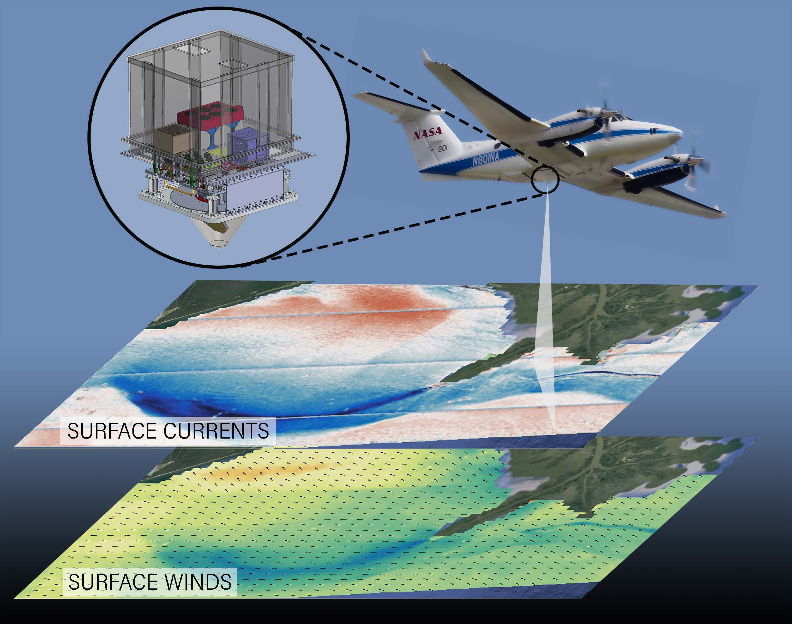The wind drives Ekman surface currents, but surface currents also modulate wind momentum transfer through kinematic effects [4,5], and through modulation of the air-sea boundary layer by the temperature of the water carried by the currents [6,7]. Therefore, to fully understand air-sea interactions, a critical mechanism in governing the Earth’s climate and weather, it is important to make simultaneous estimates of both winds and surface currents. Drastic improvements in our understanding of wind-driven upwelling, boundary layer dynamics, equatorial circulation, flux transport, and nutrient and pollutant advection [8] are enabled by the simultaneous measurement of submesoscale winds and total currents.

The potential for measuring ocean currents from space using two antennas has been understood since the pioneering work of Goldstein et al. [9] in along-track interferometry (ATI). Spaceborne ATI current measurements of a single radial velocity component were demonstrated by Romeiser et al. [10] using Shuttle Radar Topography Mission (SRTM) data. Subsequently, Freeman et al. [11] proposed getting full vector currents by spinning the two antennas. The ATI technique, although promising greater precision, requires large antennas separated by a considerable distance (10 m) and suffers from either swath limitations (non-spinning antenna) or mechanical complexity (spinning two large antennas separated by a large mast). An approach that requires only one antenna to measure one velocity component was proposed by van der Kooij (unpublished) and refined by Chapron and colleagues [12]. This approach used the Doppler centroid (rather than interferometric phase) measured by a Synthetic Aperture Radar (SAR) to estimate the radial velocity along the beam direction. Chapron et al. [12] also demonstrated the need to have simultaneous vector wind estimates to enable the translation of the measured Doppler into surface currents along the look direction. Using a SAR instrument, it was not possible to obtain vector winds due to the lack of absolute calibration and the inability to retrieve wind direction using only one look direction.

The above concepts suffer from three main drawbacks: (1). radar range ambiguities that severely limit swath width; (2). unrealistic complexity/cost; and/or (3). a lack of coincident wind/wave measurements necessary for surface current estimation. Pencil-beam Doppler scatterometry overcomes all of these important problems. Problem (1) is solved by spinning a pencil beam antenna to build up a wide swath, rather than building the swath with multiple fixed antennas. Problem (2) is solved by building on the well-known scatterometer principles developed for QuikSCAT [13] with the addition of Doppler capability. Spinning scatterometer systems are mature and relatively easy to implement, certainly when compared to multi-antenna or large-baseline systems. Finally, problem (3) is solved by the use of scatterometry to measure winds using the same instrument, simultaneously.

The Ka-band radio waves transmitted by Doppler scatterometers interact with only the upper centimeter of the ocean, making measurements right at the ocean’s surface. This phenomenology differs from a typical high-frequency coastal radar installation, whose HF-band signals interact with larger ocean waves and penetrate deeper to depths of a few meters. At Ka-band, radar scattering is caused by small wind driven capillary waves that ride on top of the underlying surface current, meaning some amount of wind must be present for adequate radar return power and SNR. Additionally, because Doppler scatterometry measures the total surface velocity of small wind driven capillary waves, the motion of these small waves must be removed from all measurements of surface velocity, as must the orbital motion of larger waves, to leave behind only the underlying surface current. Removal of wave motion from Doppler scatterometer measurements can be done using an empirical model function, based on the winds measured by the same instrument.

Besides the important development of techniques, physical understanding, and models for the removal of wave motion, pencil-beam Doppler scatterometry has additional unique challenges. The technique requires precise pointing calibration and high-frequency (Ka-band) radar hardware. Overcoming all of these challenges is one of the reasons DopplerScatt was initially funded.

DopplerScatt is a first of it’s kind airborne pencil-beam Doppler scatterometer. The instrument provides a proof of concept for the measurement technique, hardware, and algorithms, and a stepping stone to a spaceborne mission. With the National Academy’s Decadal Review selection of vector ocean currents as a targeted climate observable to measure in the next ten years from space, and their suggestion of Doppler scatterometry as the means, there is wide support for a spaceborne Doppler scatterometer based on technology developed for DopplerScatt.

At the same time, DopplerScatt’s synoptic measurements of submesocale currents are a scientifically unique and useful measurement. DopplerScatt will provide the primary surface current measurements during the upcoming Earth Ventures Suborbital-3 Submesoscale Ocean Dynamics Experiment (S-MODE). S-MODE will revolutionize our understanding of ocean dynamics by surveying small scale ocean currents to determine their role in oceanic mixing, heat and nutrient transfer, and their interaction with the wind.

Section 2 of this paper presents an overall description of, motivation for, and the design of the DopplerScatt instrument, including its operating parameters, system testing, calibration, and operation. Section 3 presents deployments thus far and Section 4 discusses high level results and performance from those deployments. For full details on the processing, measurement technique, and phenomenology, which are not extensively documented here, see Rodriguez et al. 2018 [14].

2. The DopplerScatt Instrument

2.1. System Design Considerations

Two primary goals can be outlined for DopplerScatt: (1). enable wide-swath, submesoscale resolution measurement of ocean surface currents and winds from an airborne platform; and, (2). increase the technology readiness for similar spaceborne instruments. The first goal of course drives the design of the instrument, but the second goal puts additional constraints on the airborne system design that might not otherwise be necessary for airborne measurements.

The objectives of wide swath measurements and the estimation of surface currents oppose one another in a fixed-antenna radar system. In order to measure surface currents, relatively short radar pulses (and inter-pulse periods) are required, shorter than the ocean correlation time of about 1 ms. As the inter-pulse period (IPP) shortens, so too does the unambiguous swath, according to:

$$D_u=\frac{c{\tau }_i}{2sin\theta }$$

(1)

where ${\tau }_i$ is the inter-pulse period, which is nearly the same as the pulse length assuming little down time, c is the speed of light, and $\theta$ is the incidence angle. With a 1 ms IPP, the maximum unambiguous swath is about 180 km. Another important timing consideration is the broadside correlation time, which, for an airborne platform traveling at 120 m/s with a reasonably sized antenna, is about the same as the ocean correlation time. For a spaceborne platform, these swath restrictions make stationary antenna systems unacceptable for wide-swath measurements, even if multiple long antennas are used to obtain looks for vector measurements. Spinning a pencil or fan beam antenna overcomes these unambiguous swath restrictions by keeping a short IPP and building up a wide swath using the spun antenna.

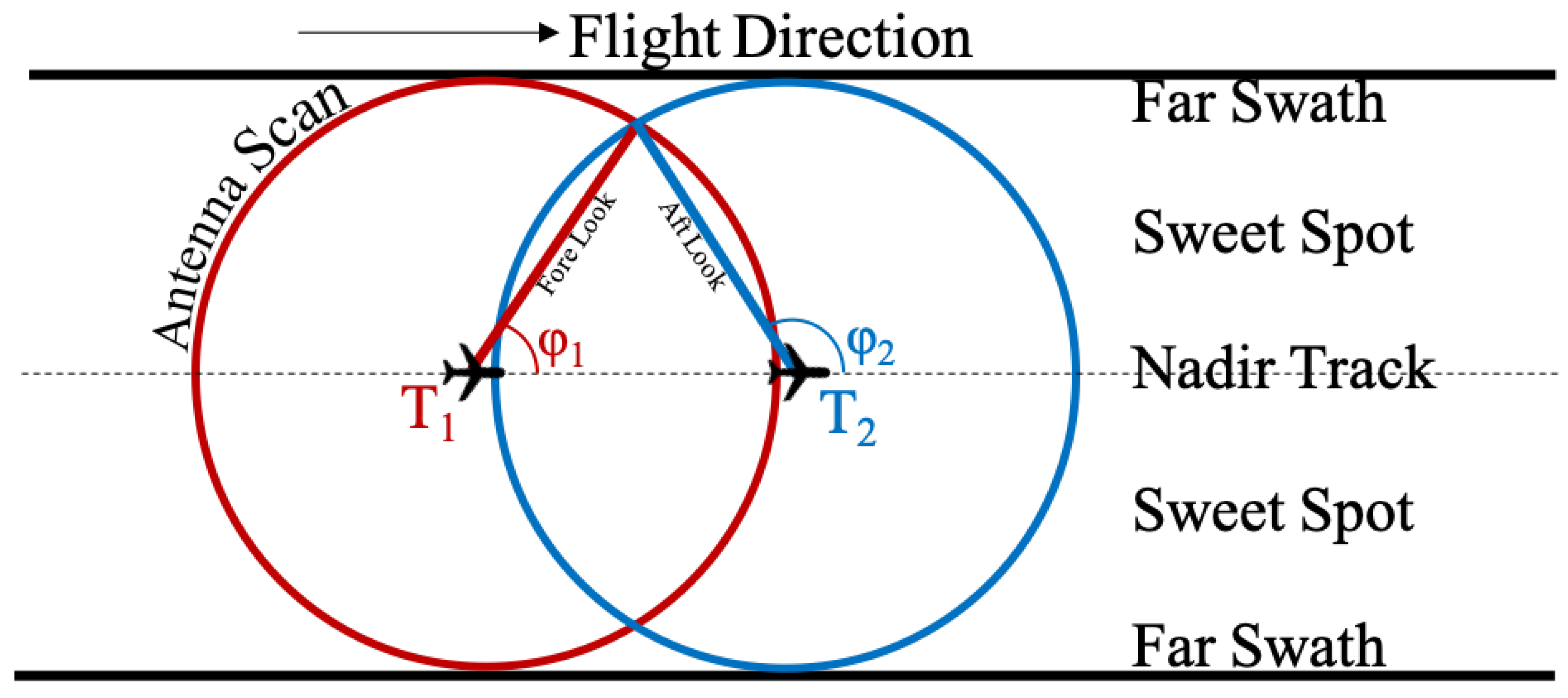
A second benefit of the spinning antenna is that it obtains multiple views of every resolution cell on the ocean surface, each from (ideally) different azimuth angles. While any one estimate of surface current speed is made radially along the look direction of the antenna, measurements from both forward and backward looks can be combined into vector measurements. The antenna rotation rate was set accordingly to to form a complete swath of both forward and backward looks. Figure 1 shows the measurement geometry and swath orientation for spinning pencil beam Doppler scatterometry.

Since Doppler scatterometry depends on the inter-pulse phase and absolute backscatter, a level of phase and amplitude stability is important between pulses and over time. A loopback calibration circuit is used, through which periodic calibration pulses are characterized. This calibration allows for automated system noise characterization and for the removal of trends over time. This method could be implemented for a spaceborne mission.

The radial velocity error requirement for DopplerScatt was set at 10 cm/s. This requirement most stringently constrains the pointing requirements for the system, in particular, the azimuth pointing knowledge. For an error in azimuth knowledge of $\delta \varphi$, the error in surface projected radial velocity is approximately given by,

$$\delta V_{rs}=V_{p}sin\varphi \delta \varphi$$

(2)

where $\varphi$ is the azimuth angle and $V_p$ is the along track platform velocity. From this, in order to meet a 10 cm/s requirement, azimuth pointing must be known to within 10${}^{-3}$ degrees. This is orders of magnitude better pointing knowledge than motor encoders can provide. Calibration of azimuth knowledge must therefore be done using DopplerScatt data itself.

The radar footprint is dependent on the transmit frequency assuming a given antenna size and measurement geometry. Higher frequencies allow for a smaller azimuth footprint, which in turn leads to lower surface current velocity noise. While the airborne instrument could likely achieve low enough noise without the use of a high frequency, a spaceborne mission would realistically require the higher gain and lower noise benefits of higher frequencies. Ka-band was chosen as the next step up in frequency from heritage scatterometers that operate at C- and Ku-bands, with the hope that the technology development for Ka-band pulsed amplifiers would prove possible in a reasonable time-frame.

One of the unknowns at the outset of DopplerScatt design was how to optimize the radar timing for the airborne instrument and how the ocean correlation time would affect the airborne and spaceborne designs. For this reason, the digital subsystem was required to generate a wide range of timings and be capable of pulsing much faster than the ocean correlation time. Fast pulses ensure that the ocean correlation time would not become a problem, and further allows for its wind speed dependence to be understood for the design of a spaceborne mission. The ability to arbitrarily set radar timings allows for trades to be made between number and length of pulses, and for investigation of the correlation coefficient between different pulses. In order to allow these types of fast and arbitrary pulse timing, a Solid State Power Amplifier (SSPA) was selected, as opposed to a Traveling Wave Tube Amplifier (TWTA) for its capability of operating at 100% duty cycle vs a typical 30% for the TWTA. On receive, the digital subsystem continuously samples basebanded signals, which, in combination with the pulsed SSPA, allows for noise estimation during times between transmit pulses and and received echoes, as well as sampling of calibration pulses.

2.2. Instrument Design and Accommodation

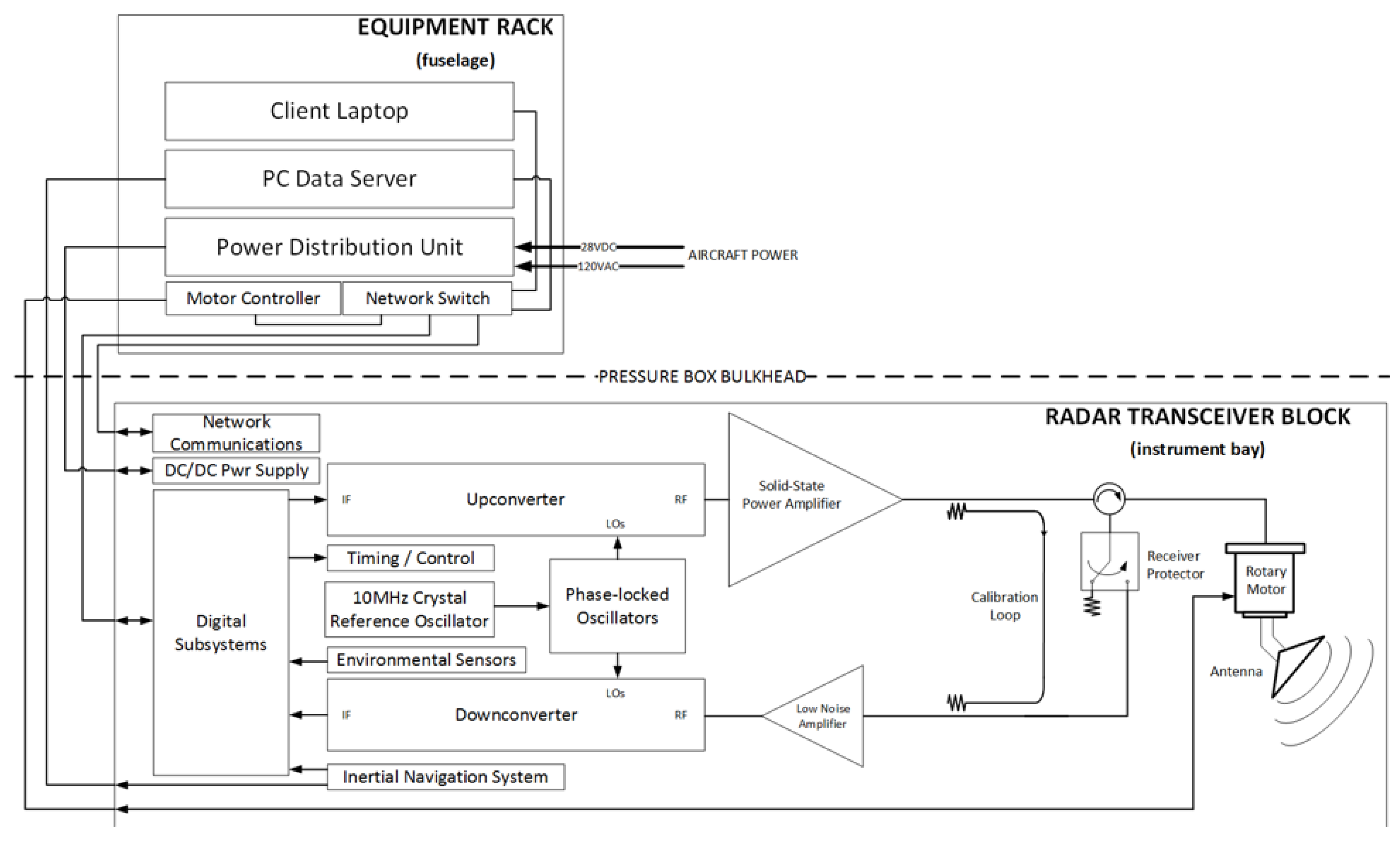
DopplerScatt is a coherent burst-mode scatterometer. As such, the high level radar block diagram for DopplerScatt is similar to a conventional scatterometer system, with the main differences residing in the digital subsystem, where the signal phase is retained. The radar block diagram is shown in Figure 2.

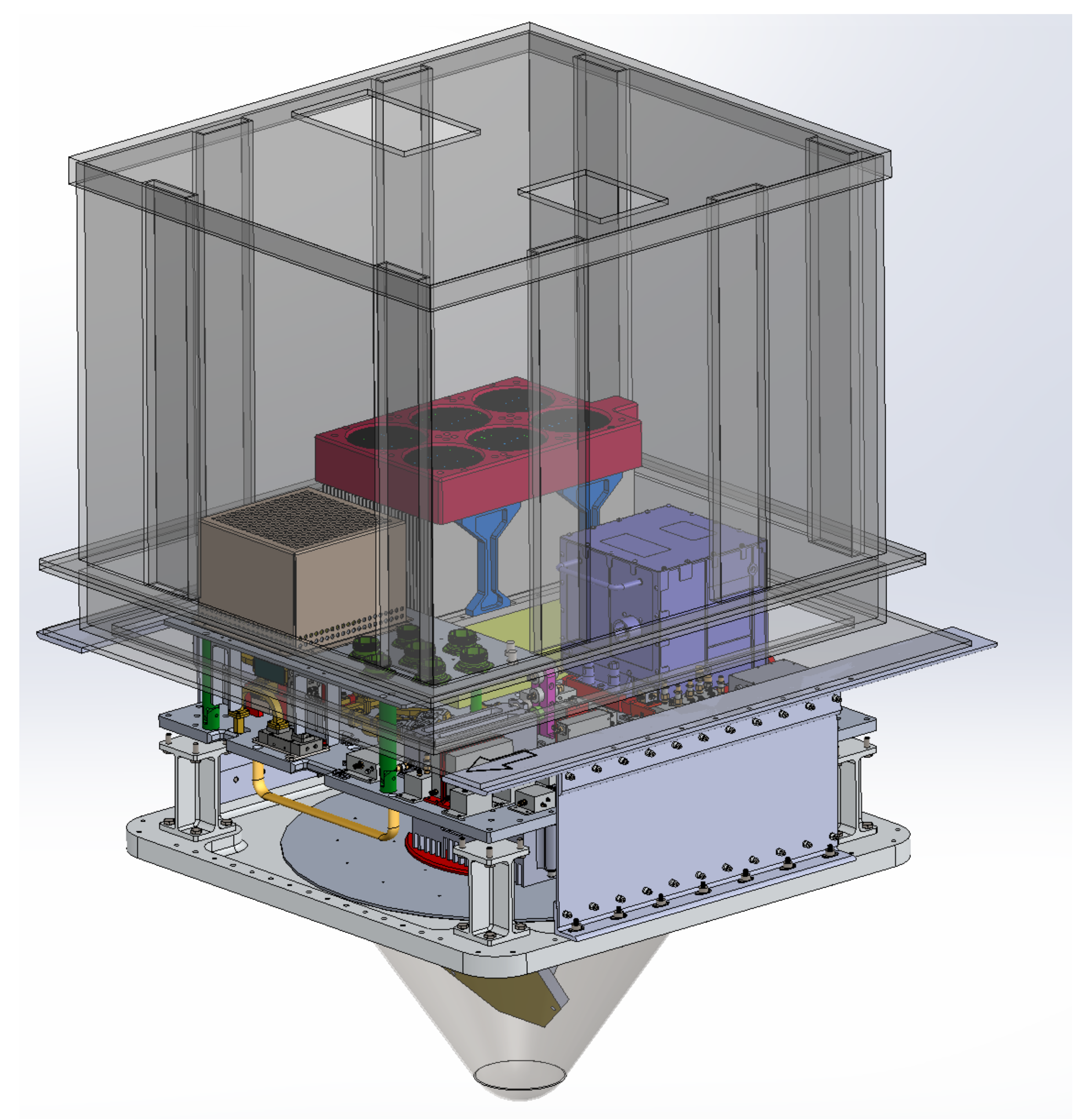
The instrument consists of two physically distinct sections: the equipment rack, inside the pressurized aircraft cabin, and the radar transceiver block, which sits in the unpressurized instrument port in the underside of the host aircraft. Starting in the digital subsystem, transmit pulses are defined at a low power, intermediate frequency (IF), before being upconverted to Ka-band and sent through the 100 Watt Solid-State Power Amplifier (SSPA). The signal at this point is at high frequency and transmitted via waveguide to a single-channel Ka-band rotary joint, through the spun antenna platform, and finally through the waveguide slot array antenna. The return signal is then sent through a low-noise amplifier, downconverted back to an intermediate frequency, and digitized in the digital subsystem. Once digitized, signals are sent across a pressure bulkhead to the equipment rack inside the aircraft. The equipment rack holds servers where raw data is redundantly recorded across two data acquisition computers and processed in real-time to L1B products. The rack also holds the controller for the antenna spin motor, a GPS receiver module, and a control station for the radar operator.

The Remote Sensing Solutions Inc. digital subsystem consists of a central timing unit (CTU), signal digitizers, data acquisition systems, ancillary data logging, and real-time FPGA processors for digital filtering and down-conversion. It was originally based on the AirSWOT digital receiver but modified to allow radar burst mode and to correlate radar data with data from ancillary sensors. In particular, the digital system logs data from the spin motor encoder, temperature sensors, and the GPS/IMU for precise pointing, calibration, and timing.

The internal calibration loop path passes through the full receiver chain, except the rotating antenna. Transmitted pulses are attenuated and routed through the calibration loop for characterization of system noise levels, which vary over time primarily due to temperature changes. To mitigate temperature changes, all components are mounted to a heated instrument plate. During flight, a PID temperature controller controls the instrument plate to a pre-set temperature range. The temperature of individual components is also continuously tracked, since the bulk control of the instrument plate does not specifically control individual component temperatures.

Instrument position and attitude are obtained using GPS coupled with an Inertial Motion Unit (IMU) using an Applanix POSAV 610 system. The antenna rotation angle is obtained by means of an encoder, which has a nominal resolution of 88 mdeg. The accuracy of the IMU and encoder pointing are important to DopplerScatt’s data processing, since platform motion must be removed from Doppler-inferred radial velocity measurements. Any misalignment in pointing (real or due to imperfect knowledge) will project the significant airplane motion into the relatively small surface currents. We have found the Applanix POSAV 610 accuracy sufficient, and have developed methods for calibrating/correcting encoder positioning that will be summarized in the following sections and more extensively in [14].

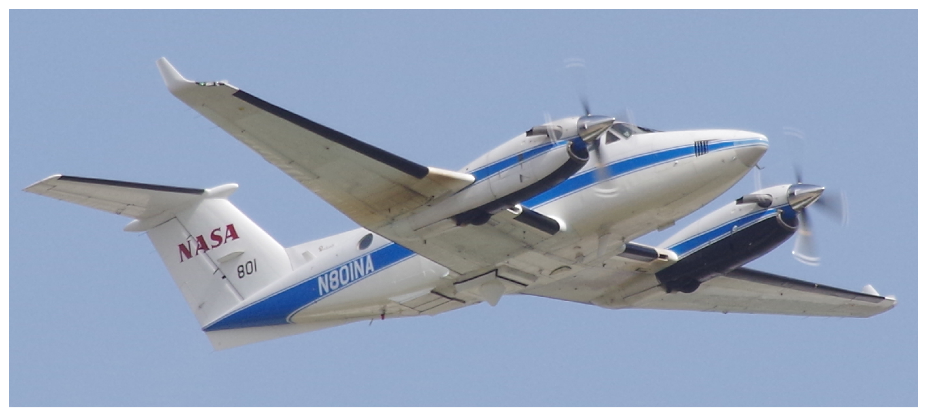
DopplerScatt is currently deployed from the NASA Armstrong Flight Research Center King Air B200 platform (NASA-801) with a nominal flight altitude of 8.5 km. This aircraft was chosen primarily for its slow flight speed that ensures adequate antenna rotational coverage across the entire ground swath, and its relatively high altitude flight capability that allows for a wide measurement swath. Figure 3 and Figure 4 show a view of the aircraft with the DopplerScatt radome and the Dopplerscatt instrument transceiver block in its flight configuration, respectively. The transceiver block is installed through a nadir-facing aircraft port, with the Ka-band transparent radome extending beneath the aircraft and the radar electronics extending up into a pressure box in the aircraft cabin. The radome and antenna extend far enough below the aircraft’s wings that they do not interfere with the antenna pattern. Radar electronics are located on the transceiver block in the unpressurized pressure-box to reduce losses in the RF subsystem and for heritage in case of future UAV operation, which would likely require unpressurized operation. The modularity shown in Figure 4 allows the instrument to be easily installed on NASA-801 in a single day. Installation into other aircraft is possible with modifications to or re-build of mounting brackets and an aircraft-specific fairing, assuming the host aircraft meets other instrument requirements. Note that the mounting brackets and fairing must be at minimum modified in order to accommodate the instrument onto new aircraft, even if that aircraft is a King Air B200, due to differences in bolt patterns and nadir-ports between seemingly similar aircraft. The combination of the host aircraft nadir port geometry and DopplerScatt mounting brackets and hardware sets the horizontal plane for DopplerScatt, which in turn sets the nadir spin axis for the antenna. It is important that this spin axis be within a few degrees of true-nadir during flight, since this angle determines the radar incidence angle. Model functions for wind and current retrieval have been trained for a narrow set of incidence angles around the nominal 56 degrees.

Wire harnessing transfers power and data across the pressure bulkhead from the control rack to the transceiver block. The pressure bulkhead requires a total of seven ports for the wire harness. Electrically, DopplerScatt requires 28 V DC and AC power from the host aircraft and an external GPS antenna connection. DC power draw is approximately 400 W and 120 V AC power draw is approximately 500 W. The dimensions, mass and power of each component are summarized in

Table 1. Instrument summary mass, power, and dimensions.

Instrument Rack Mass	102 kg
Instrument Rack Dimensions	0.56 × 0.62 × 0.95 m
Transceiver Block Mass	81 kg
Transceiver Block Dimensions	0.56 × 0.58 × 0.27 m
Wire Harness Mass	6.8 kg
28 V DC Power Draw	400 W
120 V AC Power Draw	500 W

. No data or commands are currently transmitted between the ground and instrument/aircraft, so no satellite internet connection is required. We have conducted electromagnetic compatibility (EMC) testing between the instrument and aircraft and found no noticeable interference between the two in either direction.

2.3. Configuration and Operating Parameters

In

Table 2. DopplerScatt Instrument Configuration for 5 and 10 MHz Modes.

Parameter	Value	Value
Pulse Bandwidth	5 MHz	10 MHz
Peak Power	100 W	100 W
3 dB Azimuth Beamwidth	3${}^{\circ }$	3${}^{\circ }$
3 dB Azimuth Footprint	800 m	800 m
3 dB Elevation Beamwidth	3${}^{\circ }$	3${}^{\circ }$
3 dB Elevation Footprint	1.4 km	1.4 km
Nominal boresight angle	56${}^{\circ }$	56${}^{\circ }$
Burst Repetition Frequency	4.7 kHz	3.5 kHz
Inter-pulse Period	18.4 $\mathsf{\mu }$s	30.5 $\mathsf{\mu }$s
Chirp length	6.4 $\mathsf{\mu }$s	12 $\mathsf{\mu }$s
Pulses per burst	4	2
Azimuth Looks	100	100
Range Resolution	30 m	15 m
Ground Range Resolution	36.2 m	18.1 m
Resolution in Azimuth	600 m	600 m
Nominal Platform Altitude	8.53 km	8.53 km
Nominal Swath	25 km	25 km
Scan Rate	12.5 RPM	12.5 RPM
Noise Equivalent ${\sigma }_0$	−39 dB	−38 dB

, we present only the system configuration used to obtain the results presented in Section 4, although the instrument is capable of a wide range of settings.

With a peak power output of approximately 100 W, a 3${}^{\circ }$ beamwidth antenna (inherited from the Mars Science Laboratory landing radar), and a linear frequency-modulated 5 MHz chirp, the system achieves a nominal noise-equivalent ${\sigma }_0$ (SNR=0), of about −39 dB. Upgraded hardware now allows for a 10 MHz chirp with a nominal noise-equivalent ${\sigma }_0$ of about −38 dB. These levels of nominal noise-equivalent ${\sigma }_0$ ideally allow for sampling down to wind speeds of about 2 m/s, although phenomenology may degrade wind retrieval at such low wind speeds. The antenna is a completely passive vertically polarized waveguide slot array, mechanically mounted at a nominal boresight look angle of 56${}^{\circ }$. This leads to a ground swath width of 25 km when spun about the nominal vertical axis at a rotation rate of 12.5 RPM at 8.5 km altitude.

Although the system pulse repetition frequency and spin rate allows for SAR processing, the achievable azimuth resolution using SAR will vary significantly with azimuth angle, and, at this point, data are processed in real-aperture mode to obtain more uniform sampling characteristics. Future processing upgrades will implement SAR processing with the goal of reducing measurement noise rather than increasing resolution. Current real-aperture processing leads to an azimuth footprint size of approximately 600 m. In the range direction, the 5 MHz chirp bandwidth results in a ground resolution of 36 m (18 m at 10 Mhz). The achievable ground resolution when gridding multiple looks will vary across the swath, but can lead to significant decrease in the resolution cell size, especially in the swath “sweet-spots” between the nadir track and the far-swath (see Figure 1). Current processing sets a constant ground cell size of 400 m, resulting in a decrease in noise in the sweet spots rather than an increase in resolution. The inherited 3${}^{\circ }$ beamwidth antenna is not ideal for Doppler scatterometry, especially in a spaceborne mission. Ideally, a fan beam antenna would be used to reduce the azimuth ground pattern size, which could enable higher resolution gridding.

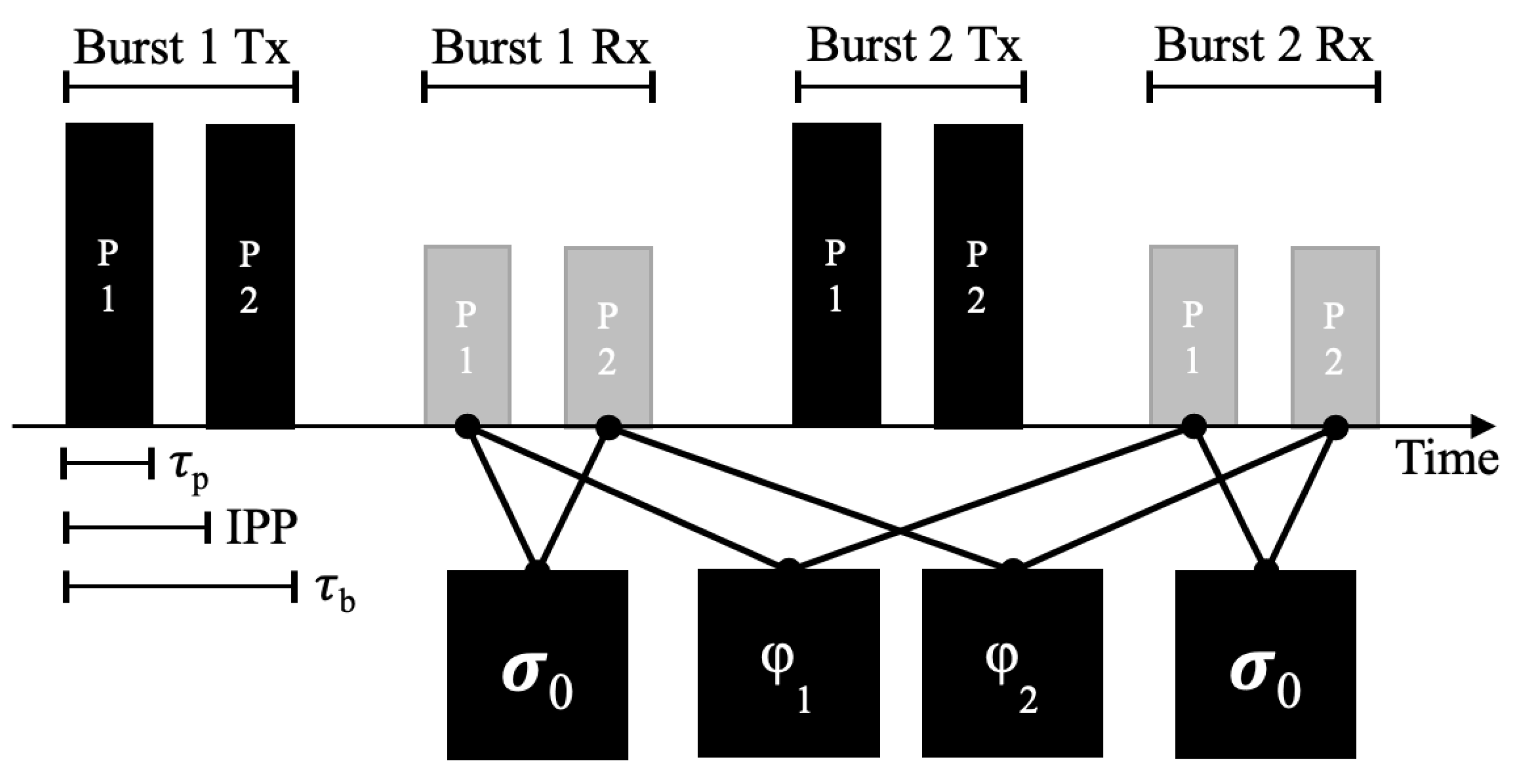
Figure 5 shows a diagram of a typical radar pulse schema for DopplerScatt, simplified to the two-pulses per burst version. Pulses from subsequent bursts are cross correlated to estimate line-of-sight radial velocity. The amplitude of all pulses in each burst are averaged together to form backscatter measurements that are later used for wind estimation. The pulsing schema used for DopplerScatt takes advantage of (and is subject to) the short signal round trip time between the aircraft and the ocean surface. From the nominal 8.5 km flight altitude, it takes light about 90 $\mathsf{\mu }$s to travel the round trip slant range. The 18.4 $\mathsf{\mu }$s inter-pulse period easily allows for multiple pulses to be transmitted before the first pulse returns to the radar. We typically choose 1-04 pulses per burst. With experience, we have moved towards fewer (1-02), longer pulses to increase the pulse compression gain. The 6.4 $\mathsf{\mu }$s pulse length leaves 12 $\mathsf{\mu }$s between each pulse as margin. This timing setup is quite different from what would be used in a spaceborne mission. For DopplerScatt, the inter-pulse period is too short to make measurements of phase differences between subsequent pulses. Instead, the phase differences are taken between pulses in subsequent bursts, which are separated by a burst repetition interval (BRI) of 0.2 ms. This BRI fully samples the Doppler bandwidth for all azimuth angles, and is shorter than the ocean correlation time of 1–3 ms [14]. At the same time, the 0.2 ms BRI is long enough for phase differences to be taken between pulses. In a spaceborne mission, the round trip signal flight time is on the order of 6 ms. With such a long flight time, longer pulse lengths and inter-pulse periods are used and allow for phase differences to be taken between pulses rather than between bursts. The pulsing schema in Figure 5 and settings in Table 2 were designed specifically for the airborne DopplerScatt instrument and the nominal flight altitude. For large changes in altitude, the pulsing schema must be adjusted accordingly.

2.4. Lab Testing

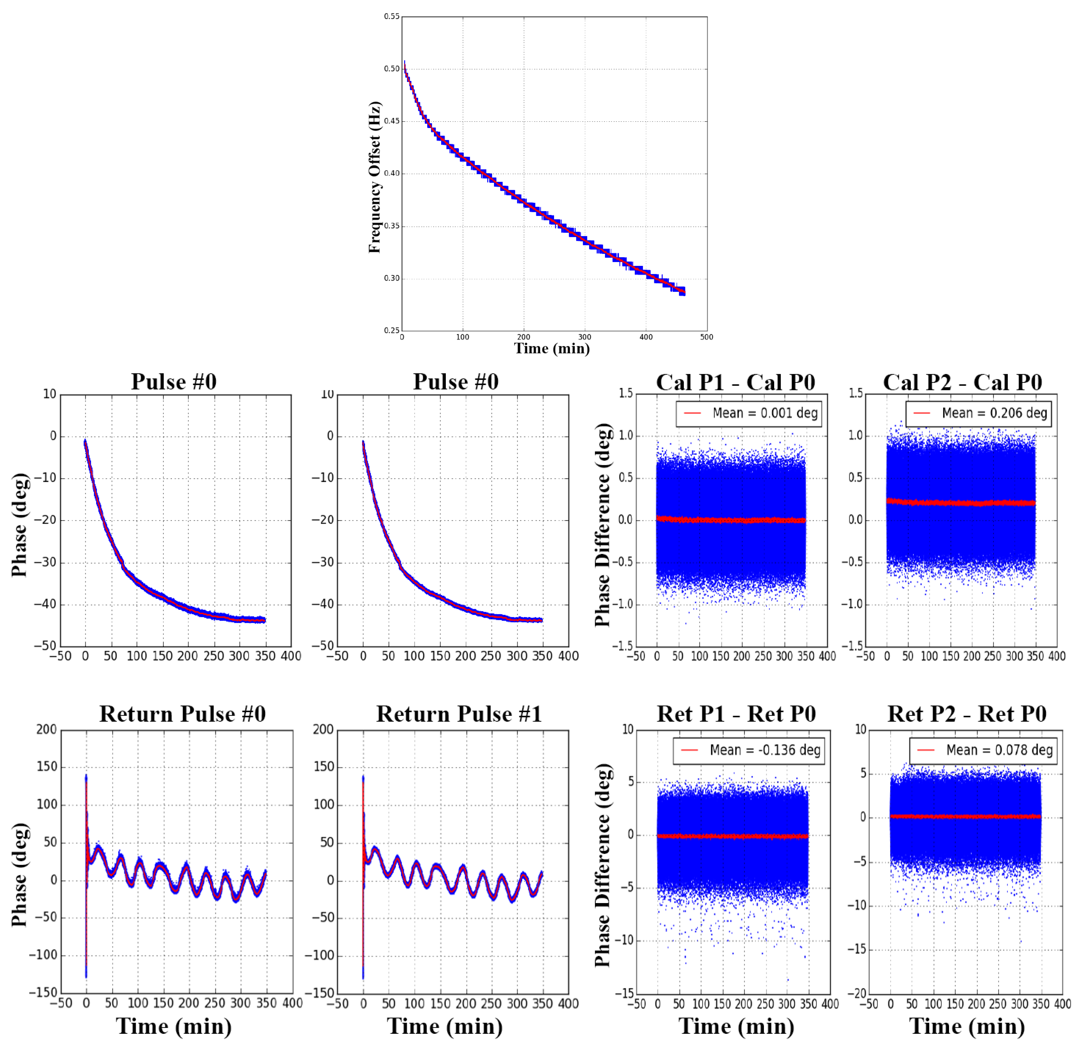
Prior to system level testing, thermal testing was performed on the receive and transmit chains, with results indicating an acceptable level of component insertion loss variability on the order of 0.1 mdB/${}^{\circ }$C. After integration, a full system characterization of the DopplerScatt instrument was performed through a series of laboratory tests, during which the gain of the transmit chain was adjusted to test saturation of the SSPA, the receiver chain was tested for linearity, and the receiver noise levels were examined and determined to have satisfactory performance. The system was tested as a whole over long periods of time where performance was evaluated for clock drift, encoder positioning, spin motor velocity, temperature variations, and phase of calibration pulses. The system’s drift of the radar master oscillator over an 8 hr data collection was tracked, recorded, and evaluated in post-processing. Figure 6 shows an acceptable level of oscillator drift during the test and a variation in pulse phase that is slow enough to be acceptable when computing pulse-pair phase differences.

The radar timing and phase performance for return pulses was tested using a Fiber Optic Delay Line (FODL) at the system’s attenuated output. FODL tests are used to test delays and settings of the radar timing in a realistic way without transmitting across a flight-like distance. FODL tests with and without thermal control concluded that temperature control in a laboratory setting does not have a significant influence on the differential phase of the pulses used to infer Doppler velocity. Phase differences between calibration pulses and delay line “echo” pulses were very stable over the collection times and their difference in standard deviation comes from their difference in SNR, as shown in Figure 6. Calibration pulses have a SNR of >35 dB while return pulses have a SNR of ∼10 dB in lab testing (operationally, the SNR depends on surface wind speeds). After FODL tests were completed, the output of the transmit chain was connected to the antenna which radiated into an RF hat (preventing RF leakage) to test for any leakage paths in the transmit chain that could affect calibration pulses.

2.5. Calibration and Metrology

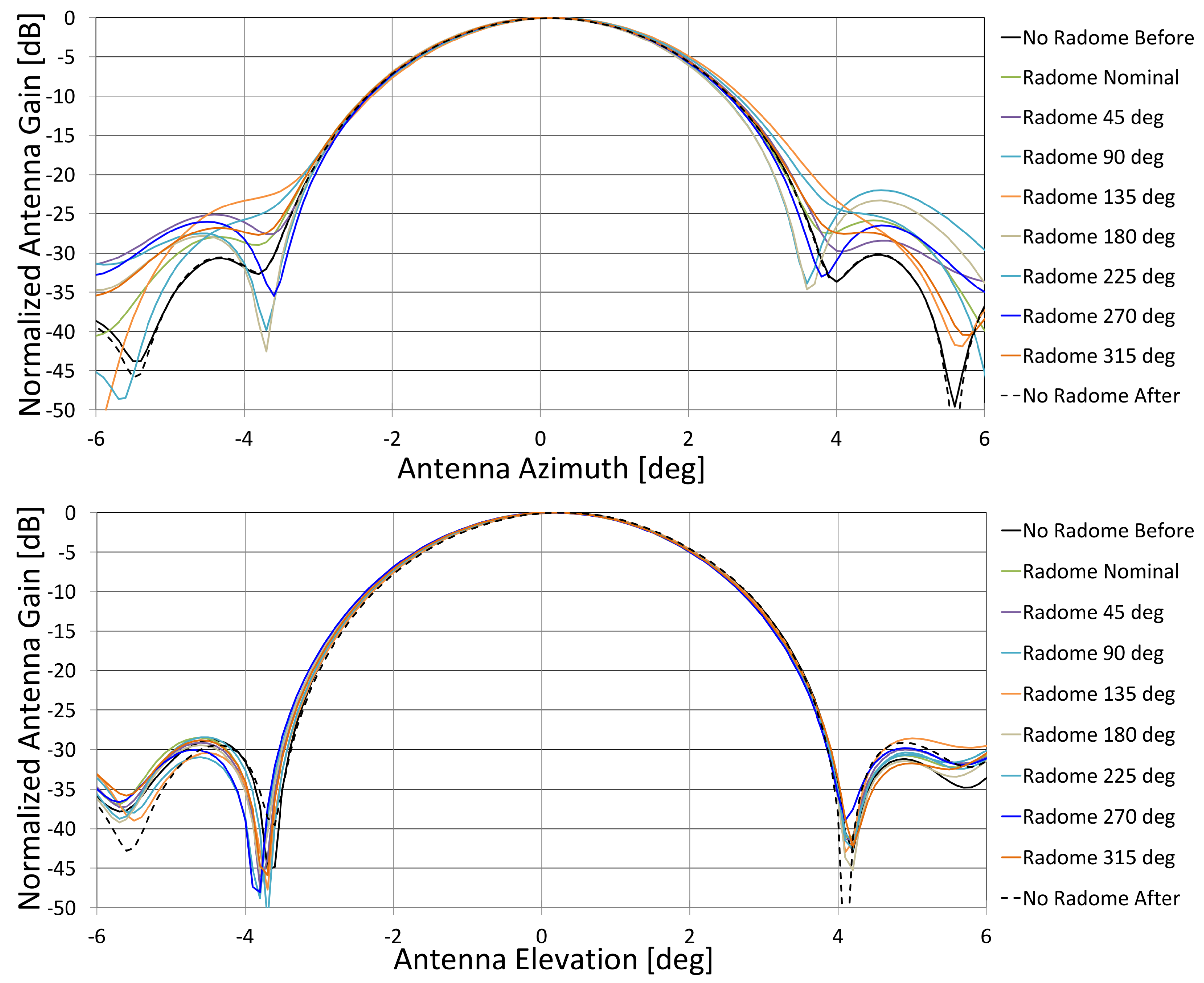
Nearfield antenna gain and phase measurements were performed to characterize the antenna’s radiation pattern and its variations due to radome losses across spin angle. These measurements found a 3 dB beamwidth of about 3 degrees and about 30 dB of sidelobe dropoff. The main lobe is nearly symmetric in shape and is well approximated by a Gaussian function with standard deviation of about 1.18 degrees in elevation and azimuth. The peak antenna gain is not exactly aligned with the antenna mechanical boresight, but instead shifted by 0.09 degrees in azimuth and 1.4 degrees in elevation. Since DopplerScatt is very sensitive to pointing knowledge, the antenna centroid, not mechanical boresight, is used during processing to determine where the antenna is pointed. Figure 7 shows the variation of the antenna pattern in antenna azimuth and elevation coordinates for various radome positions. Irregularities in the radome, due to material or manufacturing, have a more noticeable effect on the azimuth pattern than on the elevation pattern. The radome induces variable changes in gain of about 0.1 dB as the antenna rotates. This level of attenuation is consistent with High Frequency Structure Simulation (HFSS) modeling that predicts about 0.2 dB of loss. The centroid of the antenna pattern was measured to vary by about 0.1 deg, depending on radome position. Since pulse-pair phase differences are taken between pulses separated by fractions of a second, the change in radome position, and thus the difference in centroid-pointing between them, is small. For this reason, the radome modification of antenna centroid pointing is not important for pulse pair differences, although it is important for geolocation and removal of platform motion. The modification of antenna gain in the range of 0.1–0.2 dB adds noise to wind measurements, since wind direction is estimated using backscatter measurements taken from very different parts of the antenna radome. This relatively small amount of noise can be removed by using the radome-position dependent gain during processing. Laser metrology measurements were used to determine the relative positioning between the antenna and IMU, which allow for appropriate coordinate transformations during processing. The offset between the IMU and the external aircraft GPS antenna was also measured and is used during IMU setup.

In addition to calibrations done at the hardware level, DopplerScatt radar data was used to further refine pointing knowledge. Elevation angle pointing was calibrated using the relationship between radar backscatter and look-angle. We assume the slope of the relationship between backscatter and look angle should be about −0.3 dB/${}^{\circ }$ at Ka-band [15]. This calibration was updated from what was reported in [14] based on results from [15], specifically using −0.3 dB/${}^{\circ }$ rather than 0 dB/${}^{\circ }$. Surface radial velocity data from repeat-pass lines flown in opposite directions were used to estimate the absolute error in azimuth pointing, along with the variation in azimuth pointing due to inconsistencies in either the antenna spin motor velocity or the spin encoder readings. While repeat passes could not be used for spaceborne mission calibration, we believe a modified version of the calibration could be used in which “repeat passes” could be formed using the frequent overpasses near the poles. A statistical approach using a larger amount of data could also be used for spaceborne mission calibration. For DopplerScatt, each of these calibrations led to significant improvements in retrieved winds and currents, and have held constant under consistent radar parameter settings. For more information on the data-based calibration and algorithms used in processing, see [14] for an in-depth discussion.

2.6. Operations

The NASA-801 King Air B200 is capable of about five to six hours of continuous flight, typically with about an hour of takeoff and landing time; this yields maximum science data coverage of about five hours per flight. At a ground speed of about 300 km/h, and a swath width of 25 km, DopplerScatt can measure winds and currents in an area of about 7500 km${}^2$/h, or nearly 40,000 km${}^2$ in a single flight.

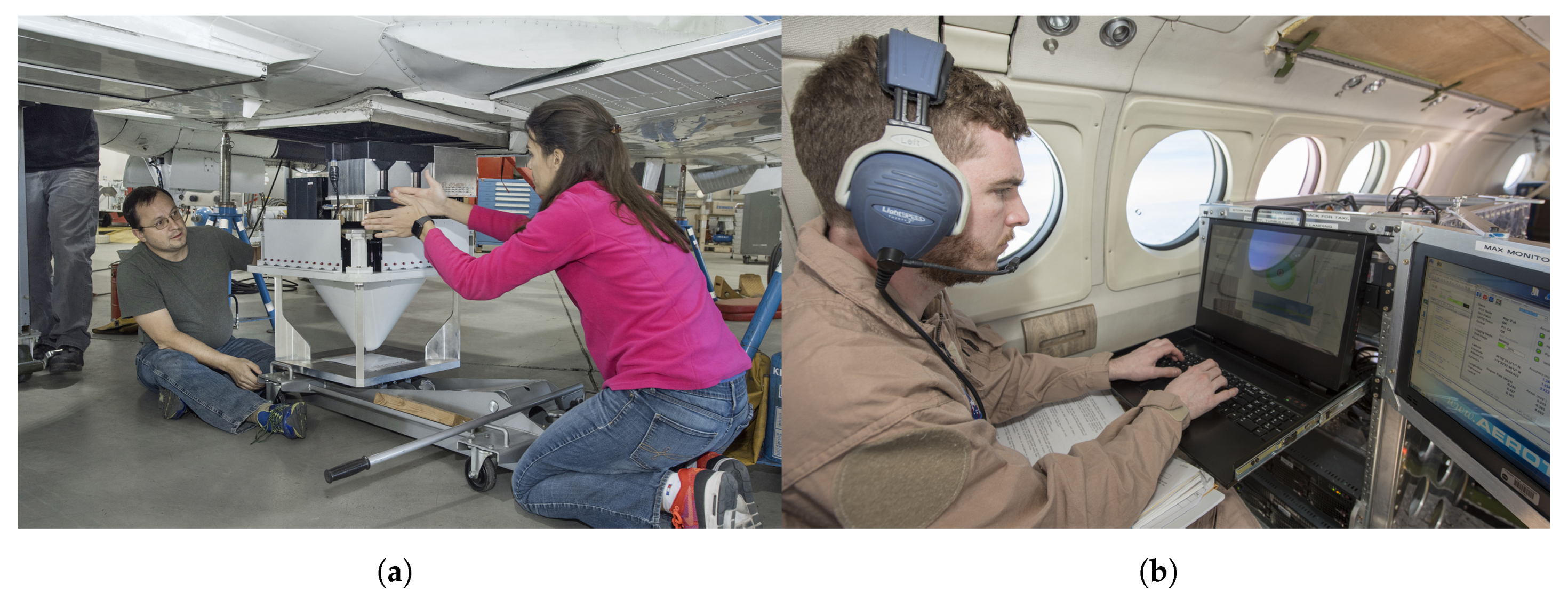
DopplerScatt is operated by a single instrument operator from inside the airplane cabin. The instrumentation rack is mounted inside the aircraft and allows for all radar functions to be controlled (Figure 8b). The instrument takes about 15 min to start up on the ground prior to take off, during which the instrument is checked out fully, with the exception of the SSPA, which is not turned on until a safe flight altitude is reached.

During flight, minimal operator control is required assuming nominal operation. Information on the health of the instrument, including temperatures, IMU/GPS quality, and antenna spin rate are displayed in real time for the operator. Received radar pulses and calibration pulses are displayed periodically as well. Two servers are installed on the instrumentation rack to redundantly record radar data. On one of these servers, data are processed up to backscatter and surface radial velocities (L1B products) and are displayed on a map for the operator (Figure 9). From this, the operator can determine whether the instrument is collecting scientifically useful data, particularly to check if winds are high enough for data to be collected. Low winds appear as very low backscatter (dark color) to the operator due to a glassy, smooth ocean surface.

After each flight, data are removed from the aircraft on solid-state hard drives for further processing and archival. From the data processed onboard the aircraft, a quick-look vector winds and currents product can be produced on a typical computer in a couple of hours. Quick-look data differs from final processing primarily in the GPS solution used for attitude knowledge. A more precise GPS solution is typically available the next day, once GPS positioning adjustment data are available. Raw DopplerScatt data are backed up before full (non-quick-look) processing. Once precise GPS data sets are available, full processing can be completed overnight using a custom cluster of eight Mac Mini computers. The cluster is designed to be easily portable during deployments in a standard “carry on” sized bag. Processing on the cluster is controlled using any laptop computer over a wireless VNC.

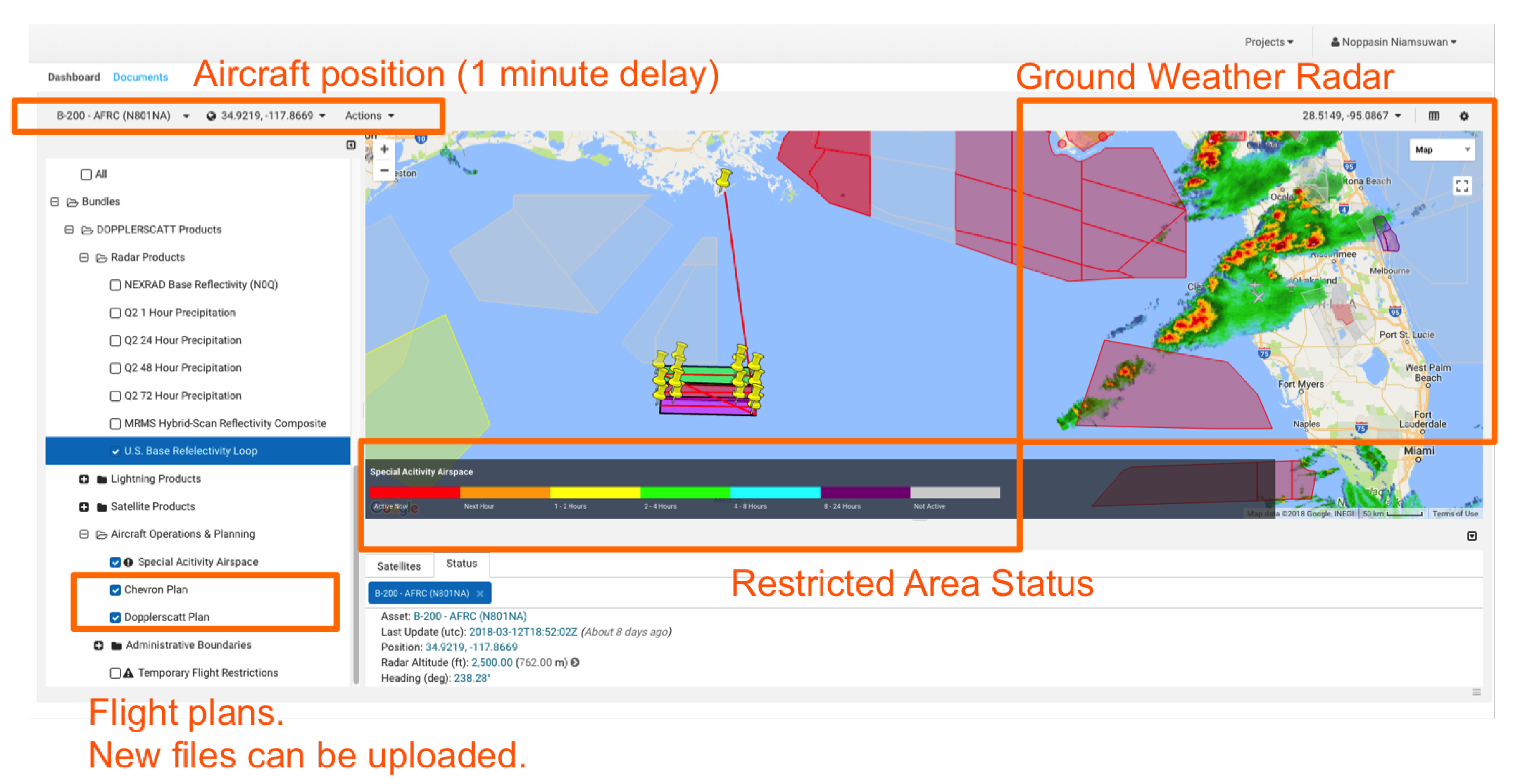
While DopplerScatt is fairly flexible, it does have a few operational constraints that should be considered when planning deployments. First, flight regions must be accessible: military and civilian flight restrictions may prevent transit and may interfere directly with a desired flight region. As with all scatterometers, wind speeds at the ocean surface must be above 2–3 m/s to receive meaningful radar returns. While clouds are typically transparent at Ka-band, rain drops are not. Rain will attenuate the radar signals and contaminate data. Winds at flight altitude can push the airplane too fast for the antenna’s spin rate, leading to skipping ground cells. This can be corrected by lowering the resolution of processed winds and currents, but should be avoided for the nominal 400 m resolution. A good rule of thumb is to avoid flight altitude winds of more than 100 km/hr. Finally, consider whether there are in-situ measurements already in place that can aid in post-flight data analysis and flight planning. Using in-situ measurements, models, and DopplerScatt’s own quick-look wind and current measurements can help determine the best time and place to fly during deployments.

Many of the above guidelines are easily followed by using the NASA Mission Tools Suite developed at NASA Ames Research Center and adapted for use with DopplerScatt. This mission planning tool allows for flight line waypoints to be imported from KML/KMZ, plotted along with the instrument ground swath, and overlaid on maps that include no-fly zones. Satellite overpasses, weather models/radar, and other in-situ data can be plotted and overlaid as well, as shown in Figure 10. During flight, MTS can track the aircraft in real time.

3. Results

Deployments

DopplerScatt’s first engineering flights were over the Rosamond dry lakebed in Southern California, where radar corner reflectors exist for calibration. After confirmation of radar functionality, flights were conducted over Lake Tahoe in California and off the coast of Big Sur, California. Ocean flights in Big Sur were the first look at the performance of the radar in a realistic environment, and, fortunately, provided high wind speed data that proved easy to process.

Since these initial engineering flights, a number of longer duration science flights have been conducted, as summarized in

Table 3. DopplerScatt deployments at of the time of writing.

Deployment Name	Location	Center Lat/Lon	Start Date	Flight Hours
Rosamond Lake 2016 part 1	Rosemond, CA	34.83, −118.05	8/6/16	2
Lake Tahoe 2016	Lake Tahoe, CA	39.09, −120.04	16/6/16	3
Rosamond Lake 2016 part 2	Rosemond, CA	34.83, −118.05	27/9/16	2
Big Sur 2016	Big Sur Coast, CA	36.11, −121.76	22/6/16	2
Portland 2016	Columbia River Mouth, OR	46.20, −124.24	13/9/16	10
SPLASH 2017	Barataria Bay, LA	28.88, −89.77	18/4/17	25
KISS 2017	Monterey Bay, CA	36.72, −122.07	1/5/17	15
Santa Barbara 2018	Santa Barbara, CA	34.30, −119.85	12/3/18	5
Chevron 2018	Gulf of Mexico	27.32, −90.19	14/3/18	20
Bay Area (SF) 2018	San Francisco Coast	37.63, −122.73	20/8/18	20

. Flights during the Submesoscale Processes and Lagrangian Analysis on the Shelf (SPLASH) experiment were flown with some coordination with the deployment of Consortium for Advanced Research on Transport of Hydrocarbon in the Environment (CARTHE) drifters [16], although the majority of drifters were deployed farther out in the Gulf of Mexico and/or carried by prevailing currents away from the DopplerScatt flight area. SPLASH results were included in [14] and will be discussed briefly in the results section here to show instrument capabilities and phenomenology. Flights during KISS were flown in coordination with a Keck Institute for Space Studies (KISS) campaign [17], which deployed sea gliders in the vicinity of Monterey Bay to study submesoscale circulation in the area. Santa Barbara flights were the first flights with upgraded 10 MHz bandwidth, and were primarily conducted to test the new configuration. Very low wind speeds made these data difficult to process and understand, although upgraded processing in response allows for some low wind capability (2–3 m/s). Deployments funded by Chevron USA, in the Gulf of Mexico, provided a look at the surface current structure of a warm-core eddy. These deployments were particularly interesting from an air-sea interaction standpoint, since the coupling between Sea Surface Temperature (SST), currents, and the wind was readily apparent over the eddy jet. The Chevron deployments were flown with Chevron in-situ and airborne assets in the area. In particular, comparisons with Fugro’s ROCIS [18], an optical airborne surface current measurement system, provided important validation and calibration. Results from the Chevron deployment will be published in 2020. Flights off the coast of San Francisco were conducted in August of 2018, in coordination with University of Washington drifter deployments and the Scripps MASS instrument. Unfortunately, weather conditions were unfavorable for both MASS and DopplerScatt. Very low winds for the majority of the deployment made processing for DopplerScatt difficult, and near-constant low cloud cover prohibited MASS from taking data coincident with DopplerScatt. Still, the San Francisco deployment proved valuable in understanding DopplerScatt’s measurement phenomenology, especially at low winds, and analysis of the data set in comparison to HF radar and drifters is ongoing today.

4. Discussion

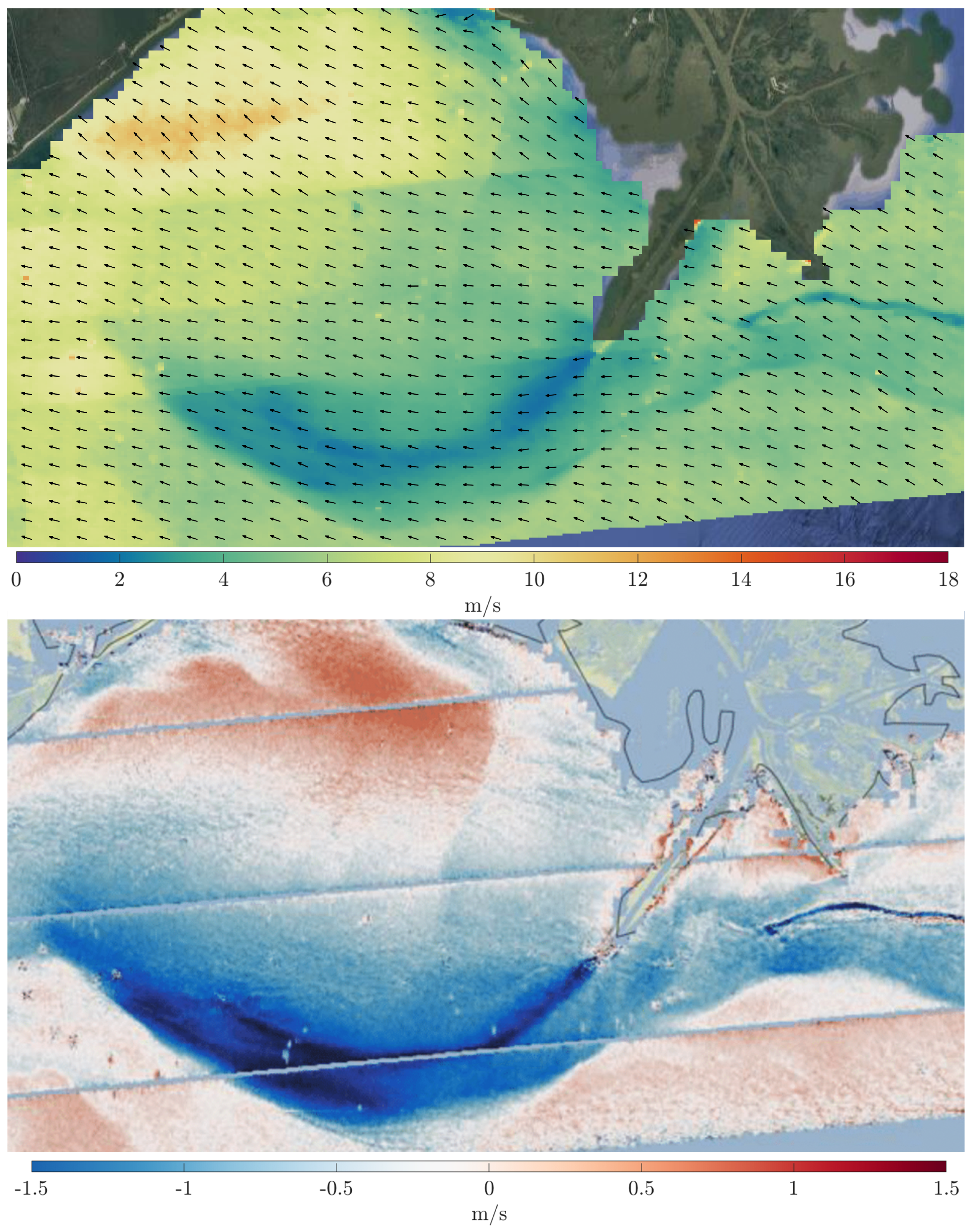
Like all scatterometers, DopplerScatt estimates the 10 m equivalent neutral wind field, which is related to the surface wind stress and is modulated by underlying surface currents and the marine-atmospheric boundary layer stability. Compared to buoys, DopplerScatt wind speed measurement performance is about 1 m/s RMS, and wind direction RMS is typically 10 degrees for winds above 3 m/s. These comparisons were complicated by the often-strong surface currents and temperature gradients in our flight areas. For example, surface currents near the mouth of the Mississippi river in the Gulf of Mexico (see Figure 11) were over 1 m/s and the cold, fresh water in the plume was nearly five degrees Celsius cooler than the surrounding ocean water. During another flight in the Gulf of Mexico, a strong warm-core eddy drove 1 m/s currents and raised sea surface temperatures by four degrees Celsius compared to the surrounding ocean. DopplerScatt measurements responded to these perturbations in measured equivalent neutral wind fields, and buoy comparisons required accounting for surface stability (due to temperature anomalies) and surface currents (which are fortunately also measured by DopplerScatt) for accurate results. This modulation is visible in Figure 11, where the Mississippi river plume has caused reduced wind speeds in DopplerScatt measurements due to the combination of cold water and strong currents flowing along the wind direction. An oil slick also led to a decrease in perceived wind speeds near the center-right of Figure 11, probably due to decreased backscatter in the presence of higher viscosity oil. An interesting side effect of using Ka-band is that the modulation due to surface surfactants is higher than at lower frequencies. Thanks to this property and our high incidence angle, it is possible to map oil slicks, and it may be possible to determine oil slick thickness based on the amount of backscatter attenuation [19].

The validation of the surface current performance of DopplerScatt is more challenging due to the lack of available high-resolution synoptic current measurements (which is exactly the problem DopplerScatt aims to remedy!). Rodriguez et al. [14] reported on qualitative comparisons against the Navy Coastal Ocean Model (NCOM), with significant agreement on the identification of frontal features. An additional experiment has been conducted in the Gulf of Mexico comparing ocean currents against those measured by Fugro’s Remote Ocean Current Imaging System (ROCIS) (Rodriguez et al., 2020, unpublished Chevron report) showing high correlations and agreements on the current speed to better than 10 cm/s, although some direction differences could be observed at lower wind speeds, potentially caused by the two instruments measuring different depth currents (DopplerScatt’s radar theoretically only penetrates the very near surface, while the ROCIS system measures dispersion caused by longer wavelength features). Detailed comparison against HF radar data on the west coast of the United States is ongoing.

5. Conclusions

The two primary reasons for building DopplerScatt were to prove the measurement technique and advance the technology necessary for a spaceborne Doppler scatterometer. The hardware used for Doppler scatterometry is by design similar to previous scatterometers, with the exception of the higher frequency Ka-band and digital systems. DopplerScatt’s Ka-band SSPA has shown that a pulsed Ka-band radar is possible with current technology. The loopback calibration shows that backscatter and phase drift due to changes in temperature (which may be more or less in space depending on design) can be accounted for. Many of the questions at the beginning of DopplerScatt’s design pertained to the high level of calibration necessary to achieve reasonable estimates of surface current velocity. A modified version of the data based calibration that calibrated DopplerScatt’s azimuth pointing could also be used for a spaceborne mission. The success of the algorithms, model functions, and phenomenological understanding developed by DopplerScatt prove that the measurement technique could be used from space.

Doppler Scatterometery offers a powerful new method for sensing submesoscale ocean vector winds and currents at synoptic scales. The DopplerScatt instrument has raised the technology readiness of essential technologies and algorithms to lay the foundation for a spaceborne winds and currents mission in the future. In the meantime, the high resolution and wide-swath synoptic views measured by DopplerScatt offer scientists unprecedented insight into the submesoscale regime.