Evaluation of Land Surface Temperature Retrieval from Landsat 8/TIRS Images before and after Stray Light Correction Using the SURFRAD Dataset

Abstract

Landsat 8/thermal infrared sensor (TIRS) is suffering from the problem of stray light that makes an inaccurate radiance for two thermal infrared (TIR) bands and the latest correction was conducted in 2017. This paper focused on evaluation of land surface temperature (LST) retrieval from Landsat 8 before and after the correction using ground-measured LST from five surface radiation budget network (SURFRAD) sites. Results indicated that the correction increased the band radiance at the top of the atmosphere for low temperature but decreased such radiance for high temperature. The root-mean-square error (RMSE) of LST retrieval decreased by 0.27 K for Band 10 and 0.78 K for Band 11 using the single-channel algorithm. For the site with high temperature, the LST retrieval RMSE of the single-channel algorithm for Band 11 even reduced by 1.4 K. However, the accuracy of two of three split-window algorithms adopted in this paper decreased. After correction, the single-channel algorithm for Band 10 and the linear split-window algorithm had the least RMSE (approximately 2.5 K) among five adopted algorithms. Moreover, besides SURFRAD sites, it is necessary to validate using more robust and homogeneous ground-measured datasets to help solely clarify the effect of the correction on LST retrieval.

1. Introduction

Land surface temperature (LST) is a key parameter in the studies of land surface progress, such as the surface energy budget, surface moisture budget, and urban ecology, which is important to nature and human health [1,2,3,4,5,6]. Remote sensing is an effective way to retrieve LST at the regional and even global scales [7,8,9]. Many satellites carry thermal infrared (TIR) sensors, such as Terra/advanced spaceborne thermal emission and reflection radiometer (ASTER), NOAA/advanced very high resolution radiometer (AVHRR), Terra and Aqua/moderate resolution imaging spectroradiometer (MODIS), Landsat 5/thematic mapper (TM), Landsat 7/enhanced thematic mapper plus (ETM+), Landsat 8/thermal infrared sensor (TIRS), and Sentinel-3/sea and land surface temperature radiometer (SLSTR). Landsat 8/TIRS is an important part of the Landsat program for monitoring surface energy and temperature. However, it was discovered to have a considerable stray light problem, which resulted in an absolute radiometric calibration error to the TIRS images [10,11]. The inaccurate radiometric calibration of TIRS, especially the excessive error in Band 11, made it difficult to apply the conventional split-window algorithms on retrieving LST from the two TIR bands of TIRS. Therefore, the data provider, United States Geological Survey (USGS), recommends the users to develop a single-channel algorithm for LST retrieval. However, several studies still proposed different split-window algorithms for this sensor [12,13,14]. In certain validation cases, the LST retrieval accuracy from the split-window algorithms was found to be better than that of the single-channel algorithm [15]. As a result, those reports have made the readers and users puzzled in choosing retrieval algorithms.

A new stray light correction algorithm proposed by Montanaro et al. [16] demonstrates great potential toward removing most stray light effects from TIRS images. The algorithm has also been refined and implemented operationally into the Landsat Product Generation System from early 2017 [17]. Gerace and Montanaro [17] selected 20 scenes (almost offshore water scenes) acquired from TIRS and MODIS onboard the Terra satellite to verify Landsat 8 brightness temperature before and after the stray light correction. They found that the absolute radiometric error of TIRS images was reduced to approximately 0.5% in Bands 10 and 11 on average [17]. This correction should benefit the LST retrieval from TIRS images. Although García-Santos et al. [18] have compared three methods for estimating LST from Landsat 8/TIRS images after the stray light correction with 21 observations, further validation in other regions is necessary for the assessment of LST retrieval accuracy after the correction. Moreover, the comparison of LST retrieval accuracy before and after the correction has not been validated using ground-measured data. Hence, the correction influence on the LST retrieval accuracy in practice remains unknown and thus requires further investigation.

With the above motivations, this study aims to clarify the following two questions: (1) Has the LST retrieval accuracy improved after the stray light correction? (2) Which algorithm (the split-window or the single-channel algorithm) is better for LST retrieval from TIRS images after the stray light correction? To answer the above questions, this paper tries to evaluate the accuracy of the LST retrieved from Landsat 8 TIRS images before and after the stray light correction by using different published two-channel split-window and single-channel algorithms. As a result, the remainder of this paper is organized as follows: Section 2 briefly presents the principles of different split-window algorithms and the single-channel algorithm; Section 3 introduces the involved Landsat 8 images and ground-measured LST and their processing; Section 4 focuses on the band radiance and LST evaluation results to answer the above-mentioned two questions; Section 5 and Section 6 provide the discussion and conclusions, respectively.

2. Landsat 8 LST Retrieval Algorithms

Five representative LST retrieval algorithms were selected for evaluation, including three two-channel split-window algorithms and one single-channel algorithm with Bands 10 and 11, respectively. These algorithms have been applied to different TIR sensors and always have been used as the reference algorithms for a new algorithm or as the state-of-art algorithms for LST validation [15,18,19,20]. Therefore, it is proper and valid to adopt these algorithms for validation in this research. Among the above algorithms, the generalized split-window algorithm was originally developed as the standard algorithm to estimate LST from MODIS TIR images and then refined in 2014 by adding a quadratic term [21]. The new version was confirmed to perform better than its previous version. Du et al. [14] applied this algorithm to conduct the LST retrieval from Landsat 8 TIRS images, and Gerace and Montanaro [17] used their algorithm to check the LST variation before and after the stray light correction. On the basis of the work of Qin et al. [22], a linear split-window algorithm for TIR images was proposed by Rozenstein et al. [13] to retrieve LST from Landsat 8/TIRS and had good performance. The split-window algorithm proposed by Jiménez-Muñoz et al. [12] was inherited from the mathematical form proposed by Sobrino et al. [23] first and modified by Sobrino and Raissouni [24], which has been developed to retrieve LST for several TIR sensors, such as AVHRR and ATSR2 [25]. The single-channel algorithm developed by Jiménez-Muñoz et al. [12] was applied to Landsat 5/TM and Landsat 7/ETM+ with a single TIR band [26,27]. Moreover, USGS recommended users to retrieve LST from Landsat 8 images with single-channel algorithm because of the serious stray light problem in Band 11. Therefore, this algorithm was also analyzed in this study. The details of the above algorithms are presented in the following part.

2.1. Three Split-Window Algorithms

A. Generalized Split-Window Algorithm by Du et al. [14]

The generalized split-window algorithm Du et al. [14] applied to two Landsat 8 TIR bands expressed as:

$$T_s=b_0+(b_1+b_2\frac{1-\epsilon }{\epsilon }+b_3\frac{\Delta \epsilon }{\epsilon })\frac{T_{10}+T_{11}}{2}+(b_4+b_5\frac{1-\epsilon }{\epsilon }+b_6\frac{\Delta \epsilon }{\epsilon })\frac{T_{10}-T_{11}}{2}+b_7{(T_{10}-T_{11})}^2$$

(1)

where T₁₀ and T₁₁ are the brightness temperatures at the top of the atmosphere (TOA) from TIRS Bands 10 and 11, respectively; ε is the average emissivity of the two bands; Δε is the band emissivity difference (Δε = ε₁₀ − ε₁₁); and b_k (k = 0, 1, …, 7) refers to the algorithm coefficients, which are obtained directly from simulation dataset on the basis of the thermodynamic initial guess retrieval (TIGR) [28] atmospheric profile database and the MODTRAN 5.2 [29] atmospheric transmittance/radiance code. Du et al. [14] calculated those coefficients independently on column water vapor (CWV) to reduce the effect of atmospheric water vapor. The CWV was divided into five subranges (0 < CWV ≤ 2.5 g/cm², 2 < CWV ≤ 3.5 g/cm², 3 < CWV ≤ 4.5 g/cm², 4 < CWV ≤ 5.5 g/cm², and CWV > 5.0 g/cm²). This method was also applied on Sentinel-3A [30] and improved by dividing the simulation data into temperature subranges. We refined these algorithm coefficients as Zheng et al. [30] did in two ways to make the evaluation more precise. First, the largest difference between the bottom air temperature (T_air) and LST used in the simulation dataset was increased from 20 K in the study of Du et al. [14] to 35 K for a barren or desert surface that probably has high surface temperature. Second, the brightness temperature of Band 10 (T₁₀) was divided into several subranges, which were used to determine the coefficients together with the CWV subranges. T₁₀ varies with LST and atmospheric conditions; thus, in accordance with the value ranges of T₁₀ under various CWV subranges, T₁₀ was divided into four subranges for 0 ≤ CWV ≤ 2.5 g/cm² as T₁₀ < 270 K, 270 K ≤ T₁₀ < 300 K, 300 K ≤ T₁₀ < 330 K, and T₁₀ ≥ 330 K. For the other four CWV subranges, T₁₀ was divided into T₁₀ < 300 K and T₁₀ ≥ 300 K.

Table 1. The coefficients b_k in different column water vapor (CWV) and brightness temperature of Band 10 (T₁₀) intervals, and root-mean-square error (RMSE) of the predicted temperature.

(1) CWV (g/cm2): [0.0, 2.5]
T10 (K)	b0	b1	b2	b3	b4	b5	b6	b7	RMSE (K)
<270	−3.1118	1.0153	0.1658	−0.3046	3.1790	8.7989	34.4917	−0.3746	0.11
[270, 300)	1.6214	0.9968	0.1739	−0.3965	4.3444	5.6164	12.8573	−0.1175	0.30
[300, 330)	7.3937	0.9788	0.1917	−0.3384	3.0247	3.2533	−14.4977	0.1291	0.30
≥330	18.0799	0.9517	0.2043	−0.2870	1.5422	3.1292	−23.0479	0.1694	0.18
(2) CWV (g/cm2): [2.0, 3.5]
T10 (K)	b0	b1	b2	b3	b4	b5	b6	b7	RMSE (K)
<300	24.9130	0.911	0.174	−0.299	6.351	3.920	−5.582	−0.064	0.54
≥300	27.4670	0.904	0.187	−0.349	5.675	2.842	−7.853	0.023	0.58
(3) CWV (g/cm2): [3.0, 4.5]
T10 (K)	b0	b1	b2	b3	b4	b5	b6	b7	RMSE (K)
<300	23.7764	0.9123	0.1443	−0.1902	7.1598	5.9811	−11.5454	−0.0597	0.71
≥300	35.3510	0.8780	0.1534	−0.2077	6.0319	5.2617	−14.5807	0.0270	1.01
(4) CWV (g/cm2): [4.0, 5.5]
T10 (K)	b0	b1	b2	b3	b4	b5	b6	b7	RMSE (K)
<300	9.6135	0.9581	0.1128	−0.1213	7.1210	6.8790	−12.5374	0.0257	0.93
≥300	36.4439	0.8736	0.1160	−0.1181	6.4603	7.0560	−16.3845	0.0305	1.32
(5) CWV (g/cm2): [5.0, 6.3]
T10 (K)	b0	b1	b2	b3	b4	b5	b6	b7	RMSE (K)
<300	50.7495	0.8021	0.0738	−0.0521	12.3012	9.7371	−15.7669	−0.3001	1.06
≥300	−63.0662	1.2070	0.0466	−0.0323	7.4367	10.3215	−13.6909	−0.0355	1.32

lists the new algorithm coefficients of Equation (1) for different combinations of CWV subranges and T₁₀ subranges and the root-mean-square error (RMSE) of the predicted temperature compared with the value in the simulation dataset.

B. Linear Split-Window Algorithm by Rozenstein et al. [13]

Based on the linear relationship between band radiance and temperature in specified temperature ranges, the linear split-window algorithm proposed by Rozenstein et al. [13] to estimate LST from Landsat 8 TIRS image is expressed as:

$$T_s=A_0+A_1{T}_{10}-A_2{T}_{11}$$

(2)

where, A₀, A₁ and A₂ are algorithm coefficients given by following equations derived from thermal radiative transfer equation [31] and linearizing Planck’s radiance function:

$$A_0=E_1{a}_{10}+E_2{a}_{11}$$

(3a)

$$A_1=1+A+E_1{b}_{10}$$

(3b)

$$A_2=A+E_2{b}_{11}$$

(3c)

In the above equations, E₁, E₂ and A are coefficients determined by pixel emissivity and atmospheric transmittance, and written as:

$$E_1=D_{11}(1-C_{10}-D_{10})/E_0, E_2=D_{10}(1-C_{11}-D_{11})/E_0$$

$$A=D_{10}/E_0, \mathrm{and} E_0=D_{11}{C}_{10}-D_{10}{C}_{11}$$

(4)

$$\mathrm{with} C_i={\epsilon }_i{\tau }_i \mathrm{and} D_i=(1-{\tau }_i)[1+(1-{\epsilon }_i){\tau }_i]$$

(5)

where, ε_i and τ_i are the pixel emissivity and atmospheric transmittance of TIRS Band 10 or 11, respectively. The atmospheric transmittance τ_i is obtained from the negative correlation with CWV by the results of MODTRAN 4.0 simulations [13], which is the only empirical fitting step in this algorithm. Therefore, different from the generalized split-window algorithm, this linear split-window algorithm is not dependent on the temperature simulation data, but the direct features of atmospheric profiles. This makes more stable simulation results of this linear split-window algorithm; because the process of temperature simulation needs more other parameters besides the atmospheric profile, such as the input LST and emissivity, while the process of transmittance simulation only needs the atmospheric profile.

C. Split-Window Algorithm by Jiménez-Muñoz et al. [12]

A split-window algorithm was introduced by Jiménez-Muñoz et al. [12] to estimate LST for the TIRS image, that is,

$$T_s=T_{10}+c_1(T_{10}-T_{11})+c_2{(T_{10}-T_{11})}^2+c_0+(c_3+c_{4}w)(1-\epsilon )+(c_5+c_{6}w)\Delta \epsilon$$

(6)

where, ε is the average emissivity of the two bands, and Δε is the band emissivity difference; they are similar to those in Equation (1). w is the CWV in g/cm², and c₀ to c₆ are coefficients. Jiménez-Muñoz et al. [12] regressed those coefficients and calculated the error of the temperature on the basis of simulation data. Their results are shown in

Table 2. Coefficients for the split-window algorithm and the land surface temperature (LST) RMSE from the linear regression by Jiménez-Muñoz et al. [12].

c0	c1	c2	c3	c4	c5	c6	LST RMSE (K)
−0.268	1.378	0.183	54.30	−2.238	−129.20	16.40	0.6

. Similar to the above generalized split-window, this algorithm also considers the quadratic term of brightness temperature difference of Bands 10 and 11, and obtains the coefficients by fitting the temperature simulation data directly.

2.2. Single-Channel Algorithm

This study used the single-channel algorithm developed by Jiménez-Muñoz et al. [27] to retrieve LST from Landsat 8 TIRS Band 10 or 11 image. This algorithm is expressed as:

$$T_s=\gamma [\frac{1}{\epsilon }({\psi }_1{L}_{toa}+{\psi }_2)+{\psi }_3]+\delta$$

(7)

where L_toa is the TOA radiance and calculated from the radiometric calibration on the observation; ε is the emissivity of Band 10 or 11; and γ and δ are two parameters given by

$$\gamma \approx \frac{T_b^2}{b_{\gamma }{L}_{toa}}, \mathrm{and} \delta \approx T_b-\frac{T_b^2}{b_{\gamma }}$$

(8)

In Equation (8), T_b is the brightness temperature of TIRS Band 10 or 11, that is, T₁₀ or T₁₁. b_γ = c₂/λ (c₂ = 1.43877 × 10⁴ μm·K; λ is the effective wavelength of TIRS, and b_γ is 1324 K for Band 10 and 1199 K for Band 11, respectively). ψ₁, ψ₂, and ψ₃ are atmospheric terms related to the atmospheric transmittance and downward and upward thermal radiance, and can be nonlinearly related to CWV. Equation (9) shows the coefficients for Band 10 that are estimated by Jimenez-Munoz et al. [12] from the Global Atmospheric Profiles from Reanalysis Information (GAPRI) database [32].

$$\left[\begin{array}{l}{\psi }_1\\ {\psi }_2\\ {\psi }_3\end{array}\right]=\left[\begin{array}{l}\begin{array}{ccc}{c}_{11}& c_{12}& c_{13}\end{array}\\ \begin{array}{ccc}{c}_{21}& c_{22}& c_{23}\end{array}\\ \begin{array}{ccc}{c}_{31}& c_{32}& c_{33}\end{array}\end{array}\right]\left[\begin{array}{l}{w}^2\\ w\\ 1\end{array}\right]=\left[\begin{array}{l}\begin{array}{ccc}0.04019\hfill & 0.02916\hfill & 1.01523\hfill \end{array}\\ \begin{array}{ccc}-0.38333\hfill & -1.50294\hfill & 0.20324\hfill \end{array}\\ \begin{array}{ccc}0.00918\hfill & 1.36072\hfill & -0.27514\hfill \end{array}\end{array}\right]\left[\begin{array}{l}{w}^2\\ w\\ 1\end{array}\right]$$

(9)

Jiménez-Muñoz et al. [12] only provided coefficients for Band 10. However, after the stray light correction, Band 11 can also be used in the single-channel algorithm. Therefore, coefficients for this band are required, as well. This study obtained the coefficient matrix C for Band 11 by using the above TIGR atmospheric profiles. The matrix is

$$C_{b11}=\left[\begin{array}{ccc}0.09874& -0.03212& 1.06497\\ -0.81391& -0.94691& -0.17172\\ -0.00676& 1.40205& -0.14864\end{array}\right]$$

(10)

2.3. Determination of Pixel Emissivity and Atmospheric CWV

The above split-window and single-channel algorithms require pixel emissivity and atmospheric CWV as input. The two parameters were both acquired using the same way to maintain constancy among algorithms.

For pixel emissivity, this study adopted the widely used normalized difference vegetation index (NDVI)-threshold method to estimate the pixel emissivity. In this method, land pixels were classified into three types on the basis of their NDVI value, namely, barren soil, fully vegetated, and partly vegetated pixels [24,33]. NDVI was calculated from atmospherically corrected ground red and near-infrared band reflectance. The emissivity of partly vegetated pixel was mainly calculated from the combination of soil and vegetation component emissivities, which are weighted by the fraction of vegetation cover (FVC). For convenience, the emissivities of barren soil and fully vegetated pixels were directly given by soil and vegetation component emissivities, respectively, on the assumption that the component emissivities slightly change in time. Finally, this method is expressed as:

$${\epsilon }_p=\{\begin{array}{cc}\hfill {\epsilon }_s\hfill & NDVI<NDV{I}_s(\mathrm{barren} \mathrm{soil})\hfill \\ \hfill {\epsilon }_{v}f+{\epsilon }_s(1-f)+4<d\epsilon >f(1-f),\hfill & NDV{I}_s\le NDVI\le NDV{I}_v(\mathrm{partly} \mathrm{vegetated})\hfill \\ \hfill {\epsilon }_v\hfill & NDVI>NDV{I}_s(\mathrm{fully} \mathrm{vegetated})\hfill \end{array}$$

(11)

where ε_p is the pixel emissivity, ε_s is the soil component emissivity, ε_v is the vegetated component emissivity, <dε> is the maximum cavity term and is set as 0.01 [34], and f is the FVC. NDVI_s is the NDVI for barren soil pixel, and its value is 0.20; NDVI_v is the NDVI for fully vegetated pixel and valued with 0.86 [35]. Ren et al. [33] improved this method by using flexible component emissivity instead of the fixed component emissivity in the original method on the basis of the different land cover types of the fine-resolution observation and monitoring of global land cover product [36].

For atmospheric CWV, the MODIS/Terra total precipitable water vapor 5-Min L2 Swath 1 km and 5 km (MOD05_L2) product was used in accordance with the location and observation time of Landsat 8. As one of MODIS standard products, the MOD05_L2 product consists of atmospheric CWV amounts estimated from two different algorithms, namely, the near-infrared and infrared algorithms. The spatial resolution of CWV data generated by the near-infrared algorithm is 1 km, whereas that of the infrared algorithm is 5 km [37]. The water vapor at 1 km was used in this study and the temporal variation between MODIS and Landsat 8 overpass time was ignored.

3. Landsat 8 Images and Ground-Measured LST

Landsat 8 images and the corresponding ground-measured data of the surface radiation budget network (SURFRAD) [38] that were usually used for in situ LST validation [15,20,39,40,41,42,43,44,45,46,47] were obtained to evaluate the different LST retrieval algorithms as mentioned above. The Landsat 8 image pairs before and after the stray light correction were obtained from the USGS website to illustrate the LST retrieval accuracy change before and after the correction. The brightness temperatures T₁₀ and T₁₁ were consequently calculated from the observation using the radiometric coefficients in the metadata file.

The SURFRAD was established in 1993 through the support of NOAA’s Office of Global Programs. The primary objective was to support climate research with accurate, continuous, long-term measurements of the surface radiation budget over the United States. SURFRAD has seven sites, but only four of them (Bondville_IL (BND), Goodwin_Creek_MS (GCM), Penn_State_PA (PSU), and Sioux_Falls_SD (SXF)) are suitable for the validation of moderate-resolution remote sensing images, such as Landsats 5 and 7, owing to the heterogeneity issues [41]. However, given that the error caused by stray light is related to the ground temperature of the surrounding area and the error is greater when the surrounding area is warm [17], the Desert_Rock_NV (DRA) site was also selected for validation to explore the effect of the stray light correction in broader temperature ranges. Since its land cover type is open shrublands, resulting in some high LST of this site. Meanwhile, DRA site has also been used in the LST validation of Landsat 8 [20] and other TIR sensors [46,47] in recent years, which can prove the applicability of the DRA site in some degree. As a result, we finally used the BND, GCM, PSU, SXF, and DRA sites to validate the Landsat 8 LST retrieval results considering heterogeneity issues and sufficient temperature range.

Table 3. The information of the surface radiation budget network (SURFRAD) sites and the image numbers under clear-sky conditions.

Site Code	Name	Geolocation	Land Cover	Clear-Sky Image Count
BND	Bondville, Illinois	40.05192°N 88.37309°W	cropland	43
GCM	Goodwin Creek, Mississippi	34.2547°N 89.8729°W	cropland	58
PSU	Penn. State Univ., Pennsylvania	40.72012°N 77.93085°W	cropland	13
SXF	Sioux Falls, South Dakota	43.73403°N 96.62328°W	grassland	31
DRA	Desert Rock, Nevada	36.62373°N 116.01947°W	open shrublands	62

lists the information of the five sites of the SURFRAD program and the number of clear-sky Landsat 8 images from its launch to August 2017 over each site. We removed the observations that had a standard deviation of temperature exceeding 1 K for 3 pixels × 3 pixels around the site center, in order to reduce the error caused by heterogeneity [41]. Finally, a total of 207 images were obtained for analysis, as shown in Table 3.

Each site provides a measurement of the upward surface TIR radiance $L^{\uparrow }$ and the downward atmospheric TIR radiance $R^{\downarrow }$ in the wavelength range of 3–50 μm every 1 min [39]. On the basis of the thermal radiative transfer equation of the near surface and the Stefan–Boltzmann law, the ground LST can be calculated as:

$$T_{s\_ground}={\left[\frac{L^{\uparrow }-(1-\overline{\epsilon })R^{\downarrow }}{\overline{\epsilon }\sigma }\right]}^{\frac{1}{4}}$$

(12)

In Equation (12), σ is the Stefan–Boltzmann constant with the value of 5.67 × 10⁻⁸ W/m²·K⁴. $\overline{\epsilon }$ is the ground broadband emissivity (BBE). BBE in 8–13.5 μm was used, because it is considered as the best wavelength range for estimating the net longwave radiation under clear sky [48,49]. To obtain this BBE, we also used the NDVI-threshold method as stated in Equation (11). However, the broadband component emissivity rather than the band component emissivity was used in Equation (11) for BBE calculation. Some details of the technique can be found in Ren et al. [33].

4. Band Radiance and LST Evaluation Results

The LST in the ground sites was retrieved from Landsat 8 images by using the above five algorithms. For simplification, the generalized split-window algorithm by Du et al. [14], the linear split-window algorithm by Rozenstein et al. [13], and the split-window algorithm by Jiménez-Muñoz et al. [12] were denoted as SW_Du, SW_Rozenstein, and SW_JM, respectively. The single-channel algorithms were denoted as SC_10 for using Band 10 image and as SC_11 for using Band 11 image. This section focuses on the LST evaluation results in two aspects, namely, the band radiance comparison before and after the stray light correction and the LST retrieval result comparison.

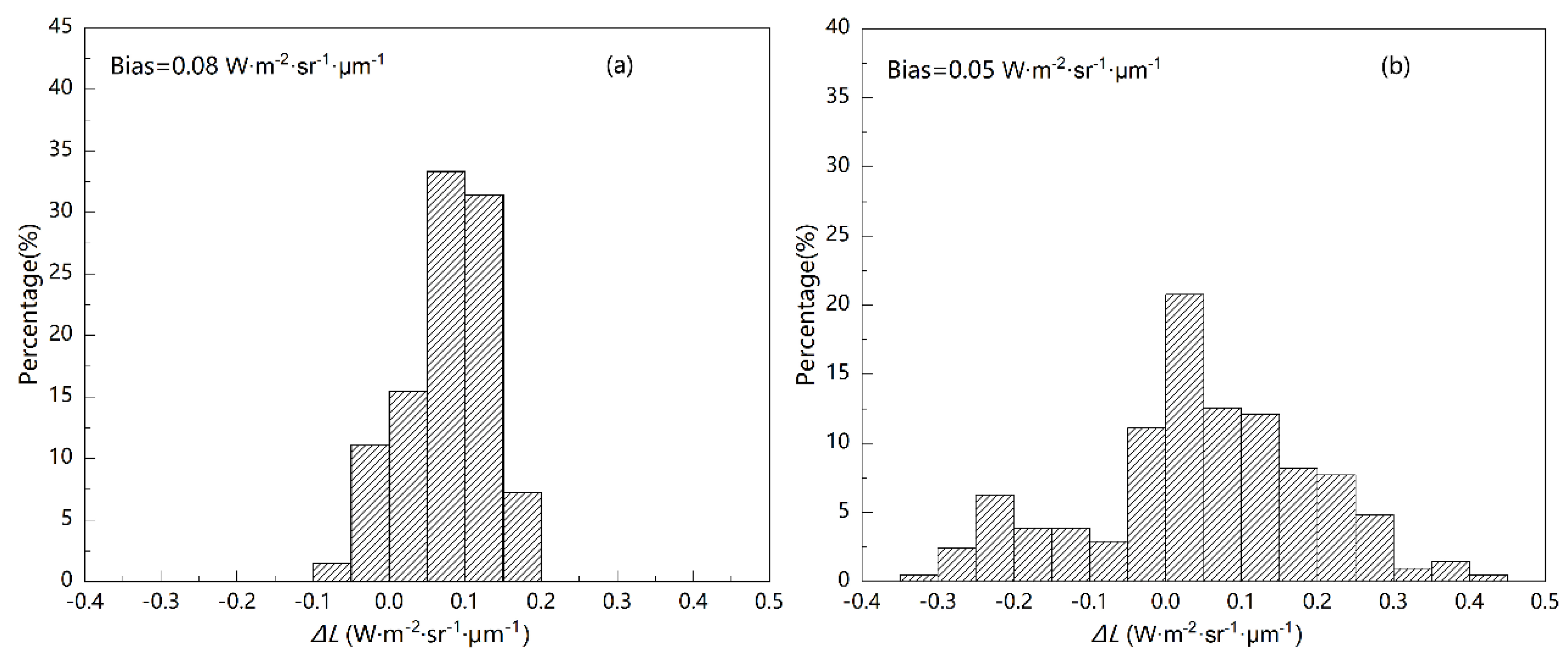
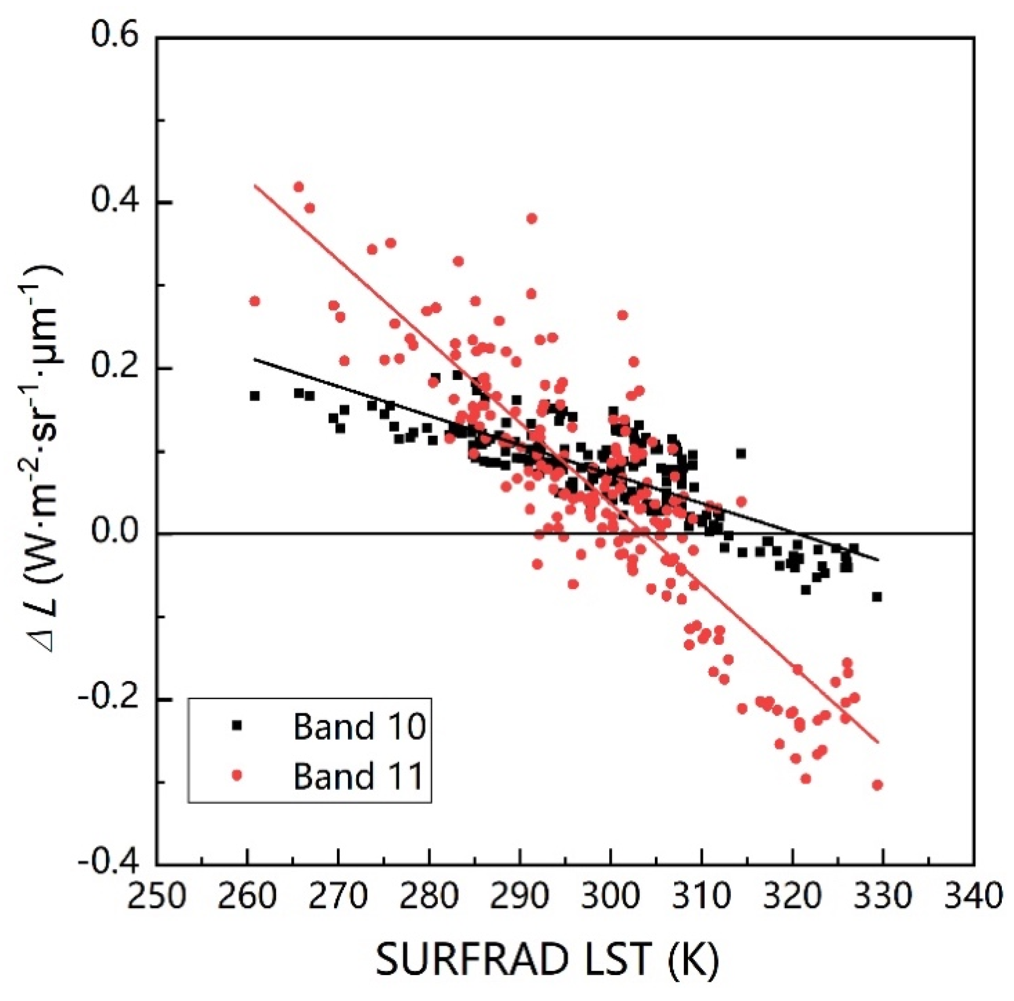
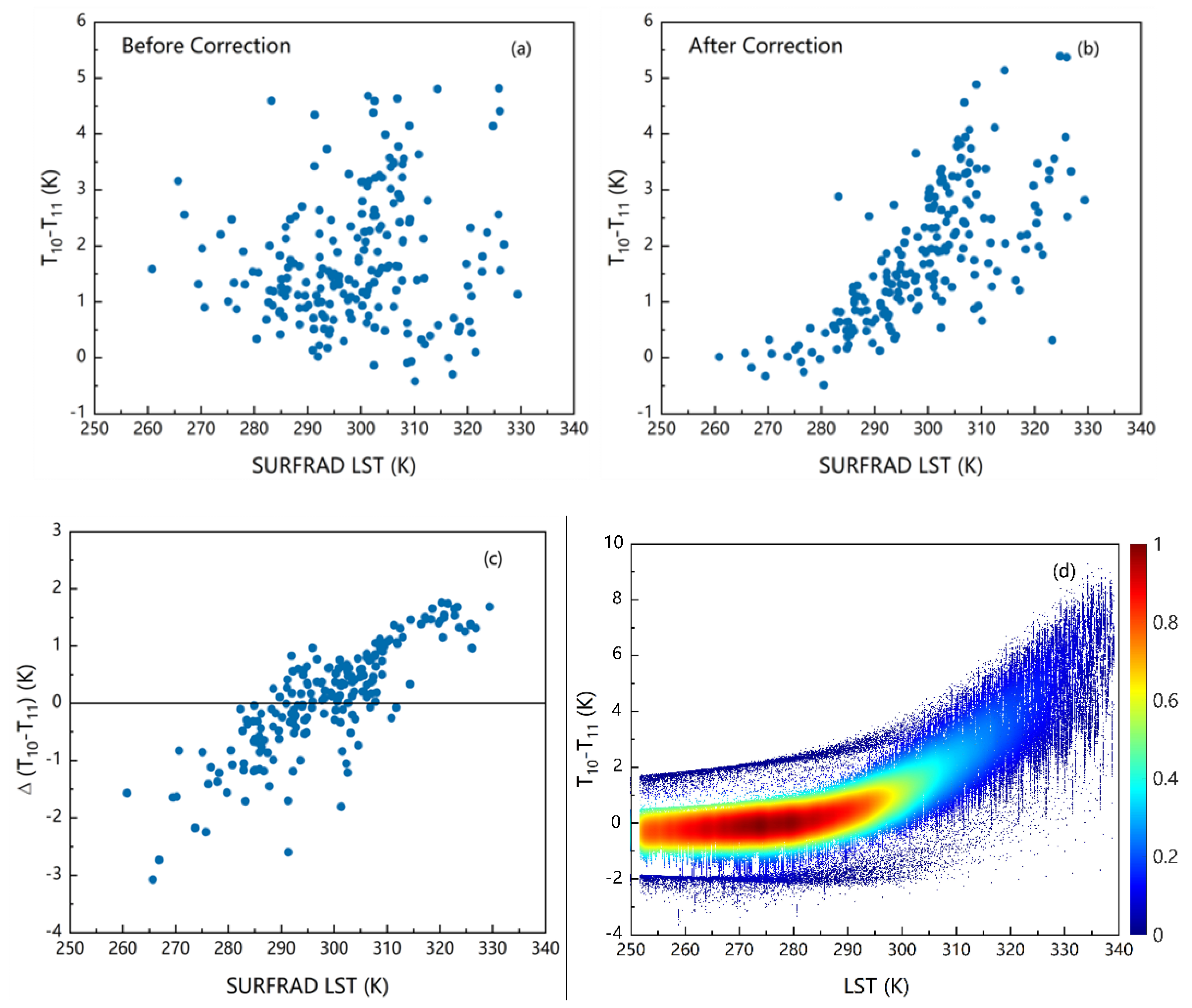
4.1. TOA Radiance Comparison Before and After the Stray Light Correction

After the stray light correction, some changes in band TOA radiance should be observed. On the basis of the above clear-sky Landsat 8 images over the ground sites, we investigated the band TOA radiance changes caused by the stray light correction. From the 207 images over the five sites, Figure 1a shows the TOA radiance difference (ΔL) of Band 10 before and after the stray light correction, and Figure 1b is the case of Band 11. The bias of both bands turned out to be slightly positive, which meant that the TIRS data became minimally “hotter” after the stray light correction in general. For Band 10, the histogram of ΔL was mostly concentrated larger than zero, with a bias of 0.08 W·m⁻²·sr⁻¹·μm⁻¹. A general positive TOA radiance change was observed for this band, although such a change was unremarkable. For Band 11, ΔL showed a broader distribution but had a similar bias with Band 10, indicating that the stray light on Band 11 was corrected in a larger scale and the variance of correction was also greater than that of Band 10.

The effect of stray light is related to LST [17], hence, the relationship between correction results and LST is necessary to explore. As stated in Section 3, the LST calculated from the SURFRAD data was regarded as the reference LST for the evaluation. Figure 2 shows the scatter plot between ΔL caused by the stray light correction and SURFRAD ground LST (SURFRAD LST). A negative correlation was firstly observed, and the radiance of Band 11 was found to have a more significant negative relationship between ΔL and SURFRAD LST than that of Band 10. In the low LST range of 260–280 K, the stray light correction of Band 11 was 0.2–0.4 W·m⁻²·sr⁻¹·μm⁻¹, which was larger than that of Band 10. In the LST range of 290–300 K, the stray light correction of the two bands became nearly the same, with a value of approximately 0.1 W·m⁻²·sr⁻¹·μm⁻¹, corresponding to a temperature difference of approximately 0.7–0.8 K. For LST > 310 K, the absolute value of the stray light correction of Band 10 was smaller than that of Band 11. Such modification can result in a remarkable effect on the final LST retrieval, especially for the single-channel method. This study analyzed this effect, as stated in the following Section 4.2, to clarify the change on LST retrieval result before and after the stray light correction.

After considering ΔL of the single band, the relationship between the two bands’ brightness temperature difference (T₁₀ − T₁₁) and the SURFRAD LST before and after the stray light correction was investigated. As illustrated in Figure 3, before the correction, the brightness temperature difference (T₁₀ − T₁₁) had no evident relationship with the ground LST (see Figure 3a). However, after the stray light correction, the brightness temperature difference (T₁₀ − T₁₁) had a significant positive correlation with the ground LST (Figure 3b) and the same trend as the simulation data (Figure 3d). This change showed that the stray light correction process not only improved TOA radiance of two TIRS bands respectively as stated in the Introduction section, but also produced a more reasonable correlation on brightness temperature of two Landsat 8 TIRS bands data. Moreover, the change Δ(T₁₀ − T₁₁) in the brightness temperature difference (T₁₀ − T₁₁) before and after the stray light correction was also found to be linearly correlated with SURFRAD LST, as shown in Figure 3c. In high temperature (LST > 320 K), the (T₁₀ − T₁₁) increased, while in low temperature (LST < 280 K), the (T₁₀ − T₁₁) decreased. Figure 3d shows that (T₁₀ − T₁₁) had an obvious relationship with LST in theory, which makes it possible to develop a split-window algorithm with the term (T₁₀ − T₁₁) to retrieve LST. Therefore, the evident and closer-to-theory relationship between (T₁₀ − T₁₁) and LST appeared after correction was expected to make the refined TIRS image more suitable for the split-window algorithm than the original TIRS image.

4.2. LST Retrieval Comparison Before and After the Stray Light Correction

This section focused on the LST retrieval evaluation before and after the stray light correction in two ways. First, the retrieved LST was compared with the ground-measured LST to check whether the LST retrieval accuracy improved after the stray light correction. Second, the LST retrieval accuracy among different split-window and single-channel algorithms was compared to find the best algorithm for retrieving LST from Landsat 8 TIRS images.

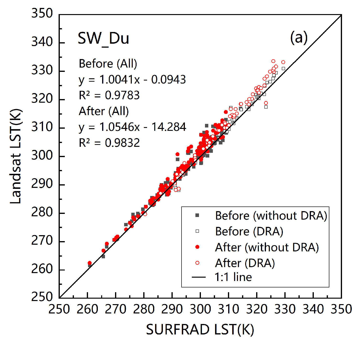
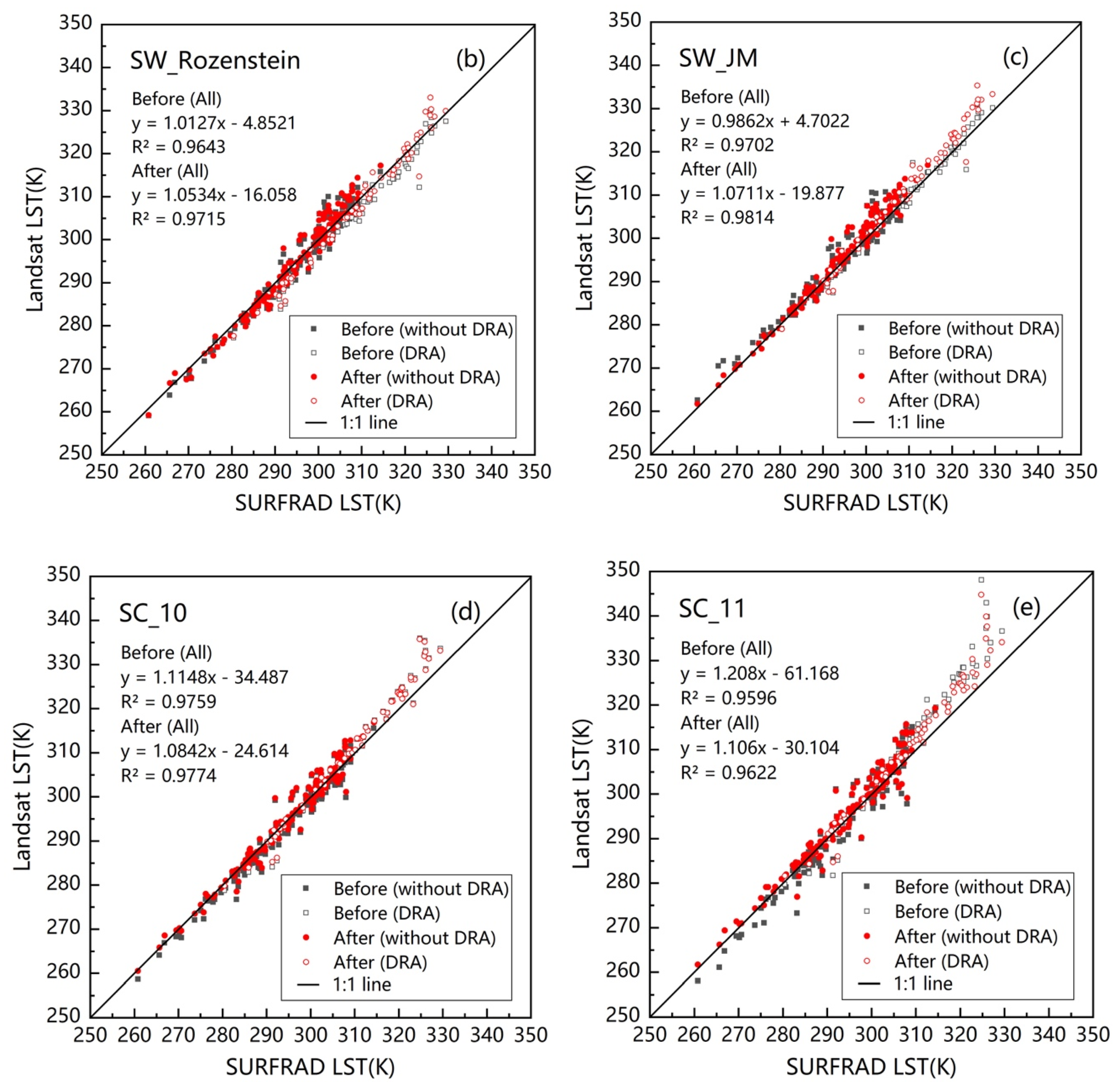
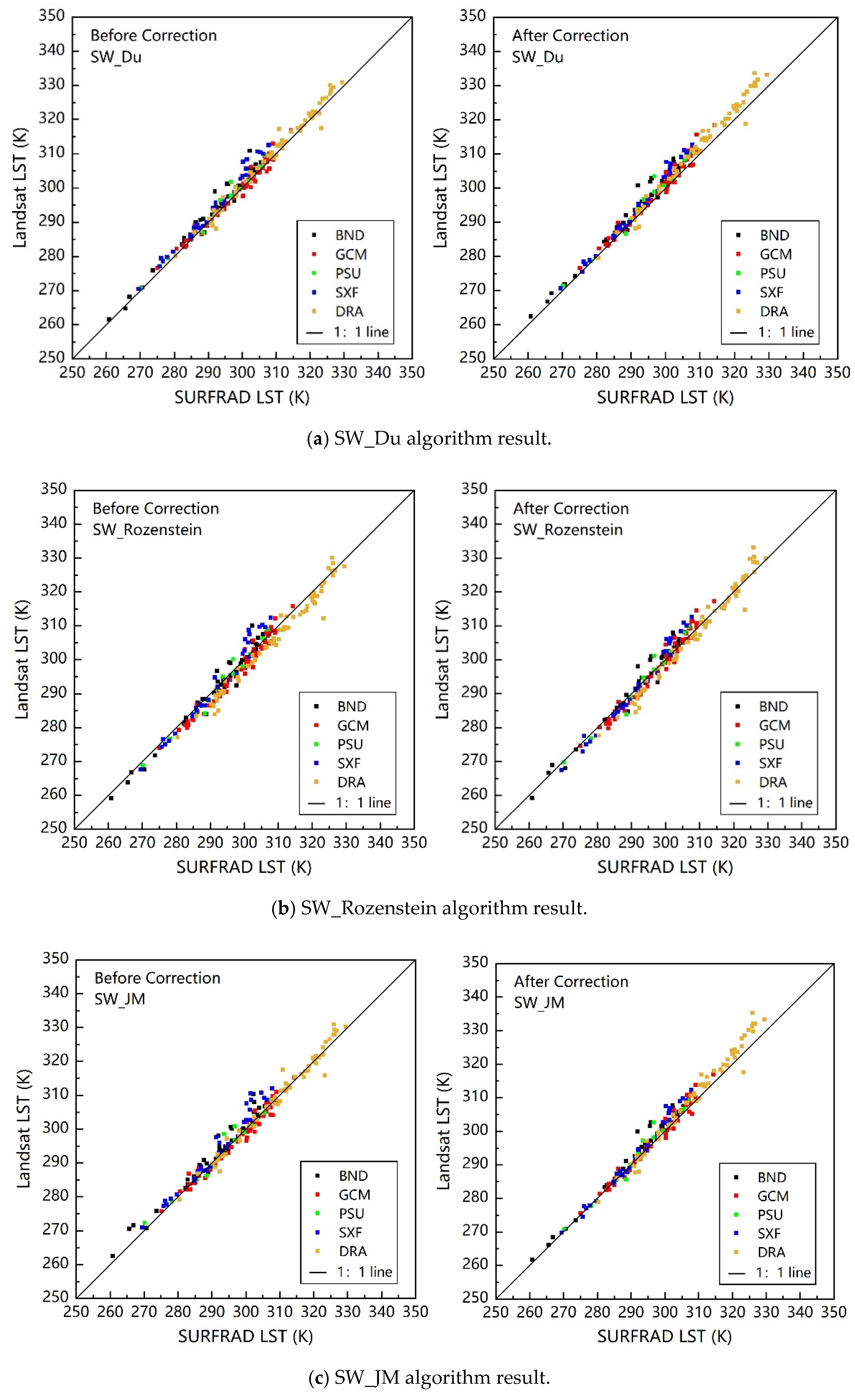
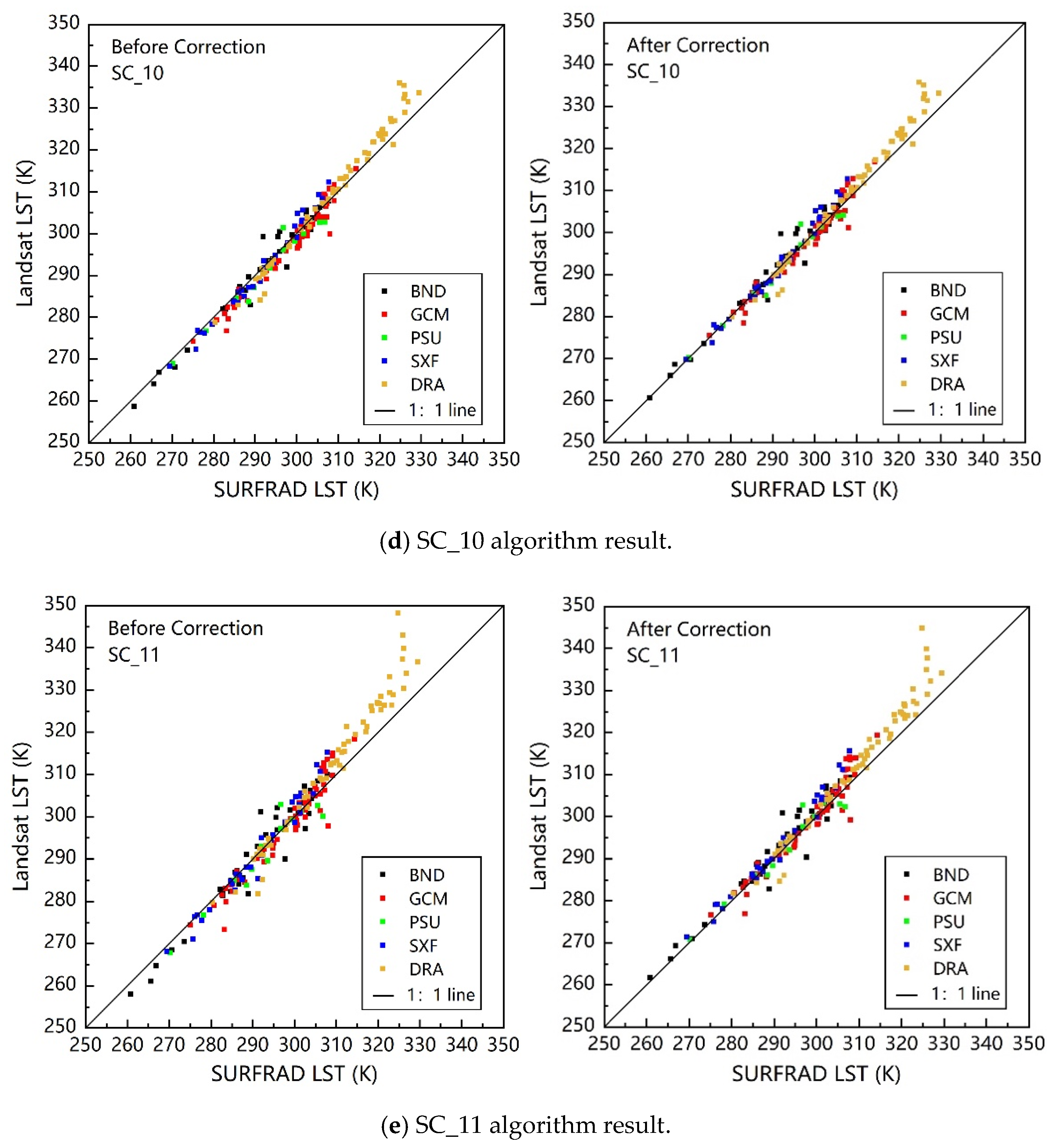
4.2.1. Overall Comparison of LST Retrieval Results

On the basis of the Landsat 8 images before and after the stray light correction, the above split-window and single-channel algorithms were used to estimate the LST over the ground sites. In accordance with the ground reference LST in different sites,

Table 4. The RMSE and bias of Landsat 8 LST retrieval from five algorithms before and after the stray light correction over all five sites.

Algorithm	Before Correction		After Correction
	RMSE (K)	Bias (K)	RMSE (K)	Bias (K)
SW_Du	2.26	1.14	2.81 (+0.55) 1	2.05 (+0.91)
SW_Rozenstein	2.76	−1.06	2.46 (−0.30)	−0.09 (+0.97)
SW_JM	2.33	0.58	2.54 (+0.21)	1.37 (+0.79)
SC_10	2.74	−0.17	2.47 (−0.27)	0.54 (+0.71)
SC_11	4.33	0.98	3.55 (−0.78)	1.59 (+0.61)

¹ The value in the bracket is the RMSE or bias change after the stray light correction compared to those of no correction.

lists the LST RMSE and bias for the five algorithms before and after the stray light correction over all five sites.

Before the stray light correction, three split-window algorithms and SC_10 nearly had RMSEs smaller than 3.0 K, which was obviously smaller than the RMSE (4.33 K) of SC_11. However, the absolute values of bias for SW_Du and SW_Rozenstein were greater than 1.0 K, indicating that the retrieved LST was slightly biased from the ground-measured LST on average. As for the single-channel algorithm, SC_10 performed better than SC_11; the RMSE of SC_10 was 2.74 K with a bias of −0.17 K, whereas SC_11 had a larger RMSE of 4.33 K. From the RMSE and bias, the performance of SW_JM exhibited the best results among the five methods before the stray light correction, with an RMSE of 2.33 K and a bias of 0.58 K. After the stray light correction, the RMSEs of all algorithms were less than 4.0 K. The least RMSE was nearly 2.5 K, which was obtained by SW_Rozenstein, SW_JM, and SC_10. Among the three algorithms, the biases of SW_Rozenstein and SC_10 were within 0.6 K; therefore, these two algorithms may be the best algorithms to retrieve LST after the stray light correction. SC_11 still had the worst performance to retrieve LST from the Landsat TIRS images, with an RMSE of 3.55 K and a bias of 1.59 K.

The comparison of the retrieved results of all sites before and after the stray light correction indicated that the absolute changes in RMSE and bias for the five algorithms were all within 1.0 K, which showed only slight changes in retrieved LSTs after the stray light correction on average. For the split-window algorithms, the RMSE of SW_Rozenstein decreased by 0.3 K, whereas that of SW_Du and SW_JM increased minimally after the stray light correction. For the single-channel algorithm, the RMSE of two bands both decreased, indicating an improved performance of the single-channel algorithm for Landsat 8 TIRS after the correction. The RMSE of SC_11 decreased most among the five algorithms but was still larger than 3.5 K. However, the bias of all algorithms increased greater than 0.6 K, showing that retrieved LSTs were overestimated after the stray light correction on average, and the correction might be biased.

Figure 4 demonstrates the comparison of LST retrieval from the five algorithms before and after the stray light correction. Moreover, because of the particularity of the DRA site mentioned in Section 3, its result is shown separately with different symbols. From Figure 4, it was found that the retrieved LST highly linearly correlated to the ground-measured LST, with coefficients R² larger than 0.95 for all cases. For the three split-window algorithms (Figure 4a–c), the retrieved LSTs from the corrected images were generally higher than those from uncorrected images, especially at high ground surface temperature. In the case that the retrieved LST before the correction was higher than the ground LST, the accuracy of LST retrieval naturally decreased if the retrieval LST was higher after the correction. For the SW_Du algorithm (Figure 4a), most retrieved LSTs before correction were higher than ground LST. After correction, the retrieval error was greater in most cases. For the SW_Rozenstein algorithm (Figure 4b), when ground LST was higher than 315 K, the retrieved LST before correction was lower than the ground LST for most cases. Although the retrieved LST after correction was higher than that before the correction (similar to the SW_Du algorithm), the accuracy of LST retrieval increased after the correction, which was different from the SW_Du algorithm. For the SW_JM algorithm (Figure 4c), under low-temperature conditions (LST < 290 K), the retrieved LST became lower after the correction. Consequently, the over-high retrieved LST before the correction was getting closer to the ground LST, leading to the improvement of retrieval accuracy. However, under high-temperature conditions (LST > 300 K), the retrieved LST after the correction became higher in general, resulting in a larger error. With the opposite accuracy change of low and high temperatures, the RMSE change of the SW_JM algorithm finally became very small and was only half of that of the SW_Du algorithm, as presented in Table 4 (+0.55 K for the SW_Du algorithm and +0.21 K for the SW_JM algorithm). For the single-channel algorithm (Figure 4d,e), the retrieved LST after the correction increased at low temperatures but decreased at high temperatures, compared to that of before the correction. The LST change of the SC_11 algorithm was more evident than that of the SC_10 algorithm (−0.27 K for SC_10 and −0.78 K for SC_11), and the scatter plot result of both algorithms were getting closer to the 1:1 line. This finding explained the details of accuracy increase in single-channel algorithms for the two TIRS bands, as shown in Table 4.

The single-channel algorithm is a theoretically derived algorithm; accordingly, the accuracy changes of SC_10 and SC_11 can be used to check whether the TIRS data are better after the stray light correction. Table 4 indicates that the errors of the SC_10 and SC_11 algorithms were reduced, meaning that LST retrieval results got better after the stray light correction and the SC_11 improved more. Combined with the change in the band radiance before and after the correction, the difference of retrieved LST can be analyzed clearly. Figure 2 in Section 4.1 illustrates that the TOA radiance of the two bands after the correction increased at low temperatures and decreased at high temperatures, resulting that the retrieved LST was closer to the ground LST of the single-channel algorithm on two bands. This finding from SURFRAD sites provided the proof supporting that the stray light correction improved not only the TIRS data quality as stated in previous study [17] but also the LST retrieval accuracy in practice. However, the validations over more robust and homogeneous ground-measured datasets, such as desert and water sites, are still needed to clarify the sole effect of the stray light correction on LST retrieval.

Since the DRA site had heterogeneity issues and high ground temperature cases (all from DRA when SURFRAD LST > 320 K) that had distinguishing features in the result of validation in Figure 4, the analysis excluding the DRA site is also necessary to help understand the effect of the stray light correction.

Table 5. The RMSE and bias of Landsat 8 LST retrieval from five algorithms before and after the stray light correction over all sites excluding DRA.

Algorithm	Before Correction		After Correction
	RMSE (K)	Bias (K)	RMSE (K)	Bias (K)
SW_Du	2.40	1.30	2.71 (+0.30) 1	1.97 (+0.68)
SW_Rozenstein	2.43	−0.42	2.30 (−0.13)	0.32 (+0.74)
SW_JM	2.47	0.82	2.27 (−0.20)	1.22 (+0.40)
SC_10	2.41	−0.83	2.11 (−0.31)	0.10 (+0.93)
SC_11	3.20	−0.17	2.84 (−0.36)	1.02 (+1.19)

¹ The value in the bracket is the RMSE or bias change after the stray light correction compared to those of no correction.

lists the temperature RMSE and bias of the five algorithms calculated from data of all sites excluding DRA.

From Table 5, when excluding high ground temperature cases of DRA, there were some differences from the results including DRA in Table 4. Except the SW_Du, the RMSE of the other four algorithms all decreased little and RMSEs of five algorithms all were within 3.0 K after the correction. The decreases on RMSE of SC_10 and SC_11 were both around 0.3 K, narrowing the gap of the RMSE change on SC_10 and SC_11 in Table 4. This indicated that the correction and improvement of single-channel algorithm on Band 11 were greater than Band 10 in a high ground temperature range, which was consistent with the result in Figure 2 and Figure 4d,e. However, the RMSE change of split-window algorithms was different from Table 4, especially for SW_JM, which will be analyzed in detail in the Discussion section. Considering the high temperature cases in the practical use, this paper finally kept the DRA site in the statistical analysis to make the conclusion more universal.

4.2.2. Comparison Results over Each SURFRAD Site

On the basis of the comparison results over all ground sites, we can determine the overall change on LST retrieval from different algorithms before and after the stray light correction. However, these sites are different from one another in the land cover type and homogeneity degree, and those differences may cause confusion in understanding the validation results. Therefore, further analysis of the results over each site is necessary.

Table 6. The RMSE and bias of the LST retrieved from Landsat 8 TIRS images on five sites before the stray light correction.

Algorithms	BND		GCM		PSU		SXF		DRA
	RMSE (K)	Bias (K)	RMSE (K)	Bias (K)	RMSE (K)	Bias (K)	RMSE (K)	Bias (K)	RMSE (K)	Bias (K)
SW_Du	2.64	1.76	1.50	0.20	1.90	1.10	3.41	2.80	1.88	0.78
SW_Rozenstein	2.34	−0.04	2.27	−1.37	1.98	−0.50	2.96	0.87	3.41	−2.56
SW_JM	2.61	1.53	1.68	−0.52	2.06	0.61	3.48	2.44	1.97	0.01
SC_10	2.30	−0.42	2.56	−1.49	2.67	−1.54	2.18	0.15	3.37	1.36
SC_11	3.17	0.03	3.27	−0.33	3.34	−1.44	3.05	0.40	6.21	3.67

lists the temperature RMSE and bias of retrieved LSTs from the five algorithms using the Landsat 8 images before the stray light correction over each site.

Table 7. The RMSE and Bias of the LST retrieved from Landsat 8 TIRS images on five sites after the stray light correction.

Algorithms	BND		GCM		PSU		SXF		DRA
	RMSE (K)	Bias (K)	RMSE (K)	Bias (K)	RMSE (K)	Bias (K)	RMSE (K)	Bias (K)	RMSE (K)	Bias (K)
SW_Du	3.04(+0.40) 1	2.39(+0.63)	2.16(+0.66)	1.43(+1.23)	2.65(+0.75)	1.83(+0.73)	3.13(−0.28)	2.48(−0.32)	3.05(+1.17)	2.21(+1.43)
SW_Rozenstein	2.33(−0.01)	0.71(+0.75)	2.07(−0.20)	−0.09(+1.28)	2.13(+0.15)	0.24(+0.74)	2.69(−0.27)	0.58(−0.29)	2.79(−0.62)	−1.07(+1.49)
SW_JM	2.52(−0.09)	1.72(+0.19)	1.77(+0.09)	0.67(+1.19)	2.26(+0.20)	1.02(+0.41)	2.70(−0.78)	1.67(−0.77)	3.07(+1.10)	1.70(+1.69)
SC_10	2.19(−0.11)	0.42(+0.84)	2.05(−0.51)	−0.43(+1.06)	2.07(−0.60)	−0.47(+1.07)	2.12(−0.06)	0.88(+0.73)	3.16(−0.21)	1.56(+0.20)
SC_11	2.87(−0.30)	1.22(+1.19)	2.82(−0.45)	0.58(+0.91)	2.48(−0.86)	−0.02(+1.42)	2.98(−0.07)	2.01(+1.61)	4.81(−1.40)	2.91(−0.76)

¹ The value in the bracket means the RMSE and bias change after the stray light correction compared to those of no correction.

provides the results after the stray light correction. Figure 5 presents the scatter plots between the retrieved LST and ground LST.

Table 6 indicates that before the correction, the four other algorithms performed better than SC_11 over BND, GCM, and PSU sites, and their temperature RMSEs were within the range of 1.5–2.7 K. From Table 7, after the correction, the temperature RMSEs of the single-channel algorithm of two bands decreased over the three sites. However, the temperature RMSE change of the split-window algorithms was not the same. The RMSE of SW_Du for the three sites evidently increased, that is, 0.40 K for BND, 0.66 K for GCM, and 0.75 K for PSU. By contrast, the RMSE of the two split-window algorithms (SW_Rozenstein and SW_JM) over the three sites changed minimally. The temperature bias of all algorithms of the three sites increased, indicating that the retrieved LST was higher after correction on average. Figure 5 depicts that the ground LST of these sites was lower than 310 K; in this temperature range, most of the radiance of Bands 10 and 11 was increased (Figure 2). Therefore, the retrieved LST results were consistent with the change in radiance.

Table 6 presents that the GCM and PSU sites were suitable to retrieve LST using split-window algorithms before the stray light correction. The RMSEs of the three split-window algorithms on the two sites were within the range of 1.5–2.3 K, which were generally smaller than those of the single-channel algorithms of both bands. After the correction, with an increase on RMSEs of the split-window algorithms and a decrease on RMSEs of the single-channel algorithms, the superiority of the split-window algorithms in retrieving LST for the two sites disappeared. SC_10 had the smallest RMSEs with a small bias over the PSU site, similar to the result obtained over the BND site. At the GCM site, SC_10 also showed no weakness compared with some split-window algorithms.

For SXF, before the correction, the performance of the split-window algorithms was worse than that of SC_10 (Table 6), and the SW_Du and SW_JM algorithms even had larger RMSEs than that of SC_11. The combined analysis of Figure 5a–c implied that for the split-window algorithms on SXF, when the ground LST was in the range of 300–310 K, the retrieved LST was obviously higher than the ground LST, corresponding to the poor performance of the split-window algorithms on SXF. After the correction, the obvious error had disappeared, indicating an improvement in the split-window algorithms in retrieving LSTs (the RMSE of three split-window algorithms decreased and the biases of split-window algorithms were closer to 0.0 K). Nevertheless, they still exhibited worse results than SC_10.

Although DRA was unsuitable for accurate validation because of heterogeneity, as mentioned in Section 3, DRA still could reveal important information of the effect of the stray light correction because of its high ground surface temperature, as illustrated in Figure 5. Its RMSE of SC_11 was very large before correction and reduced by 1.4 K after correction. The large RMSE in Figure 5e was caused by the poor performance of SC_11 at high temperature, and the improvement was due to the lower radiance correction at high temperature on Band 11 (Figure 2). This comparison result confirmed the good stray light correction of Band 11 at high-temperature conditions.

In conclusion, the biases of five algorithms increased on most cases after the correction, except for three split-window algorithms on SXF and SC_11 on DRA. However, the RMSE changes were complicated of different split-window algorithms on different sites. SW_Du and SW_JM mostly kept a similar change trend on GCM, PSU, SXF, and DRA, but their RMSEs increased after the stray light correction except on SXF. The RMSEs of SW_Rozenstein decreased on these five sites, except the PSU site, showing the better performance of SW_Rozenstein after the correction on most cases. The RMSEs of the single-channel algorithms decreased over all sites after correction. SC_10 had the smallest RMSEs and good biases on BND, PSU, and SXF after the stray light correction, and its RMSEs were approximately 2.1 K on these sites. The performance of SW_Rozenstein was close to that of SC_10 after the correction in RMSE and bias, but the accuracy of SW_Rozenstein was better than that of SC_10 for the DRA site. Therefore, similar to SC_10, SW_Rozenstein was also a better algorithm than other two split-window algorithms to retrieve LST for Landsat 8 after the stray light correction.

5. Discussion

After the stray light correction, the single-channel and split-window algorithms showed different accuracy changes in different directions and ranges. The RMSE of single-channel algorithms of two bands all decreased on each site, but none of the three split-window algorithms showed the same change (all increased or all decreased) on the five sites. Moreover, different split-window algorithms had different accuracy changes on overall sites, and even the same split-window algorithm (SW_JM) had increasing RMSE on all sites when including the DRA site but decreasing RMSE excluding the DRA site. The first confusing point is why split-window algorithms had such complicated accuracy changes that seemed to have no regularity. Secondly, when focusing on some specific temperature ranges, for instance, the high temperature (>320 K), the change of retrieved LSTs by split-window algorithms before and after the stray light correction was unreasonable. Figure 2 in Section 4.1 shows that the TOA radiance of the two bands after the correction was reduced under high-temperature condition (> 320 K). In the case if other factors are regarded as the same, the retrieved LSTs should have reduced in theory. However, as seen in Figure 4, under the high-temperature condition, the retrieved LSTs of the three split-window algorithms increased after the correction, which was inconsistent with the theoretical expectation. The same unreasonable retrieved LST changes occurred also in some low temperature cases of SW_Du and SW_JM.

To explain the two confusing points, we must first explain the RMSE change of these algorithms was made of two parts: the one was the performance of the algorithm before the correction; the other was the change of retrieved LST before and after the correction. From Figure 4 and Figure 5, it was easy to find that before the correction, the SW_Du overestimated LST for most cases (bias = 1.14 K (with DRA), bias = 1.30 K (without DRA)), the SW_Rozenstein underestimated LST for most cases (bias = −1.06 K (with DRA), bias = −0.42 K (without DRA)), and the SW_JM overestimated LST a little (bias = 0.58 K (with DRA), bias = 0.82 K (without DRA)). Different performance before the correction will certainly result in a different accuracy change if these split-window algorithms have the same retrieved LST change before and after the correction, just as the high temperature cases (>320 K).

Meanwhile, the brightness temperature relationship between Bands 10 and 11, such as the brightness temperature difference of two bands, has an important effect on the performance of split-window algorithms. Taking the SW_Du algorithm as an example, from its structure (see Equation (1)), the coefficients of $\frac{(T_{10}+T_{11})}{2}$ and $\frac{(T_{10}-T_{11})}{2}$ are positive based on the simulation data, and those coefficients of (T₁₀ − T₁₁)² are very small. Therefore, the influence of (T₁₀ − T₁₁)² can be ignored when analyzing the influence of the brightness temperature change on T_s. Under a high-temperature condition (LST > 320 K), as illustrated in Figure 3, the decreases in T₁₀ and T₁₁ would tend to cause a low retrieved LST, but the increase in (T₁₀ − T₁₁) would tend to increase the LST. The result from Figure 4a shows that the retrieved LST of the SW_Du algorithm after the correction was larger than that before the correction for the case LST > 320 K, indicating that the increasing effect on retrieved LST caused by an increase in TOA band radiance difference was greater than the decreasing effect on retrieved LST caused by a decrease in TOA radiance on Bands 10 and 11. The influence of brightness temperature difference finally caused the second confusing point above. Moreover, the different split-window algorithms have different structures and therefore, the brightness temperature relationship (for example the brightness temperature difference) will influence the performance of the algorithm in different degree. This can also cause the first confusing point, or more accurately, it was the different structures that resulted in a different performance of different split-window algorithms before the correction.

In the case that the RMSE change of split-window algorithms was much affected by the brightness temperature difference of two bands, the accuracy of brightness temperature (radiance) difference correction could directly determine the performance of split-window algorithms after the correction. However, the correction did not take into account the relationship between the radiance of two bands. Even though the radiance of Bands 10 and 11 got closer to the real radiance respectively and the relationship between the two bands’ brightness temperature difference and LST became closer to the theoretical result mentioned in Section 4.1, the value of the radiance difference between the two bands may still be more biased away from the real value, making the performance of split-window algorithms worse.

Therefore, the structure of split-window algorithms, the performance of split-window algorithms before the correction and the change of brightness temperature difference between Bands 10 and 11 combined together to cause the confusing results of split-window algorithms before and after the correction.

6. Conclusions

This study focused on the evaluation of LST retrieval from Landsat 8/TIRS data before and after the stray light correction on the original observations using ground-measured LST from five SURFARD sites. Three split-window algorithms (SW_Du, SW_JM, and SW_Rozenstein) and two single-channel algorithms (SC_10 and SC_11) were investigated.

The stray light correction increased band TOA radiance for low brightness temperature range (< 305 K for Band 10 and 310 K for Band 11) but decreased such radiance for a high brightness temperature range. The relationship between the two bands’ brightness temperature difference and LST became closer to the theoretical result.

The LST retrieval error of the single-channel algorithm was consequently reduced. The RMSE of the single-channel algorithm for Bands 10 and 11 decreased by 0.27 K and 0.78 K, respectively. The improvement in retrieval accuracy for Band 11 at high temperature was obvious. In the high-temperature site (DRA), the decreased RMSE of the single-channel algorithm for Band 11 was 1.40 K. By contrast, the accuracy of split-window algorithm (such as SW_Du) was unexpectedly reduced due to the variation in the brightness temperature difference of the two bands, and was unreasonably inconsistent with the change in radiance. For better use of split-window algorithms, the development of the split-window algorithms specified for Landsat 8, as well as the stray light correction on radiance relationship of Bands 10 and 11 may need more concern.

Among the five algorithms, the best two were SW_Rozenstein and SC_10. Before the stray light correction, the accuracy of the split-window algorithms was generally better than that of the single-channel algorithm. For the corrected images of overall sites, the accuracy of the SC_10 algorithm increased, whereas the accuracy of the SW_Du and SW_JM algorithms decreased, even making the accuracy of the SC_10 algorithm better than that of the SW_Du and SW_JM algorithms. After the correction, the RMSEs of SW_Rozenstein and SC_10 were approximately 2.5 K over all ground sites. In BND, GCM, PSU, and DRA sites, the RMSE of the single-channel algorithm for Band 10 was even within 2.2 K.

The results obtained in this study implied that the accuracy and applicability of the single-channel algorithm on Landsat 8/TIRS LST retrieval improved after the stray light correction. However, it still needs to be careful when using split-window algorithms to retrieve LST from Landsat 8/TIRS images. Meanwhile, it must be noted that the current results were only based on the measurements of five SURFRAD sites. Future evaluation using more ground-measured datasets over more homogeneous sites like desert and water sites remains strongly expected to clarify the quality of Landsat 8/TIRS data and the performance of different LST retrieval algorithms.

References

1. Mannstein, H. Surface Energy Budget, Surface Temperature and Thermal Inertia. In Remote Sensing Applications in Meteorology and Climatology; Springer Science and Business Media LLC: Berlin, Germany, 1987; pp. 391–410. [Google Scholar]
2. Price, J.C. The potential of remotely sensed thermal infrared data to infer surface soil moisture and evaporation. Water Resour. Res. 1980, 16, 787–795. [Google Scholar] [CrossRef]
3. Weng, Q. Thermal infrared remote sensing for urban climate and environmental studies: Methods, applications, and trends. ISPRS J. Photogramm. Remote Sens. 2009, 64, 335–344. [Google Scholar] [CrossRef]
4. Weng, Q.; Lu, D.; Schubring, J. Estimation of land surface temperature–vegetation abundance relationship for urban heat island studies. Remote Sens. Environ. 2004, 89, 467–483. [Google Scholar] [CrossRef]
5. Yuan, F.; Bauer, M.E. Comparison of impervious surface area and normalized difference vegetation index as indicators of surface urban heat island effects in Landsat imagery. Remote Sens. Environ. 2007, 106, 375–386. [Google Scholar] [CrossRef]
6. Koc, C.B.; Osmond, P.; Peters, A. Spatio-temporal patterns in green infrastructure as driver of land surface temperature variability: The case of Sydney. Int. J. Appl. Earth Obs. Geoinf. 2019, 83, 101903. [Google Scholar]
7. Mildrexler, D.J.; Zhao, M.; Running, S.W. A global comparison between station air temperatures and MODIS land surface temperatures reveals the cooling role of forests. J. Geophys. Res. Space Phys. 2011, 116, 15. [Google Scholar] [CrossRef]
8. Wan, Z.; Wang, P.; Li, X. Using MODIS Land Surface Temperature and Normalized Difference Vegetation Index products for monitoring drought in the southern Great Plains, USA. Int. J. Remote Sens. 2004, 25, 61–72. [Google Scholar] [CrossRef]
9. Tran, H.; Uchihama, D.; Ochi, S.; Yasuoka, Y. Assessment with satellite data of the urban heat island effects in Asian mega cities. Int. J. Appl. Earth Obs. Geoinf. 2006, 8, 34–48. [Google Scholar] [CrossRef]
10. Montanaro, M.; Barsi, J.; Lunsford, A.; Rohrbach, S.; Markham, B. Performance of the Thermal Infrared Sensor on-board Landsat 8 over the first year on-orbit. Earth Obs. Syst. XIX 2014, 9218, 921817. [Google Scholar]
11. Reuter, D.C.; Richardson, C.M.; Pellerano, F.A.; Irons, J.; Allen, R.G.; Anderson, M.C.; Jhabvala, M.D.; Lunsford, A.; Montanaro, M.; Smith, R.L.; et al. The Thermal Infrared Sensor (TIRS) on Landsat 8: Design Overview and Pre-Launch Characterization. Remote Sens. 2015, 7, 1135–1153. [Google Scholar] [CrossRef] [Green Version]
12. Jiménez-Muñoz, J.-C.; Sobrino, J.A.; Skoković, D.; Mattar, C.; Cristóbal, J. Land Surface Temperature Retrieval Methods From Landsat-8 Thermal Infrared Sensor Data. IEEE Geosci. Remote Sens. Lett. 2014, 11, 1840–1843. [Google Scholar] [CrossRef]
13. Rozenstein, O.; Qin, Z.; Derimian, Y.; Karnieli, A. Derivation of Land Surface Temperature for Landsat-8 TIRS Using a Split Window Algorithm. Sensors 2014, 14, 5768–5780. [Google Scholar] [CrossRef] [PubMed]
14. Du, C.; Ren, H.; Qin, Q.; Meng, J.; Zhao, S. A Practical Split-Window Algorithm for Estimating Land Surface Temperature from Landsat 8 Data. Remote Sens. 2015, 7, 647–665. [Google Scholar] [CrossRef] [Green Version]
15. Yu, X.; Guo, X.; Wu, Z. Land Surface Temperature Retrieval from Landsat 8 TIRS—Comparison between Radiative Transfer Equation-Based Method, Split Window Algorithm and Single Channel Method. Remote Sens. 2014, 6, 9829–9852. [Google Scholar] [CrossRef] [Green Version]
16. Montanaro, M.; Gerace, A.; Rohrbach, S. Toward an operational stray light correction for the Landsat 8 Thermal Infrared Sensor. Appl. Opt. 2015, 54, 3963. [Google Scholar] [CrossRef]
17. Gerace, A.; Montanaro, M. Derivation and validation of the stray light correction algorithm for the thermal infrared sensor onboard Landsat 8. Remote Sens. Environ. 2017, 191, 246–257. [Google Scholar] [CrossRef]
18. García-Santos, V.; Cuxart, J.; Martínez-Villagrasa, D.; Jiménez, M.A.; Simó, G. Comparison of Three Methods for Estimating Land Surface Temperature from Landsat 8-TIRS Sensor Data. Remote Sens. 2018, 10, 1450. [Google Scholar] [CrossRef] [Green Version]
19. Xu, H. Retrieval of the reflectance and land surface temperature of the newly-launched Landsat 8 satellite. Chin. J. Geophys. 2015, 58, 741–747. [Google Scholar]
20. Meng, X.; Cheng, J.; Zhao, S.; Liu, S.; Yao, Y. Estimating Land Surface Temperature from Landsat-8 Data using the NOAA JPSS Enterprise Algorithm. Remote Sens. 2019, 11, 155. [Google Scholar] [CrossRef] [Green Version]
21. Wan, Z. New refinements and validation of the collection-6 MODIS land-surface temperature/emissivity product. Remote Sens. Environ. 2014, 140, 36–45. [Google Scholar] [CrossRef]
22. Qin, Z.; Dall’Olmo, G.; Karnieli, A.; Berliner, P. Derivation of split window algorithm and its sensitivity analysis for retrieving land surface temperature from NOAA-advanced very high resolution radiometer data. J. Geophys. Res. Space Phys. 2001, 106, 22655–22670. [Google Scholar] [CrossRef]
23. Sobrino, J.A.; Li, Z.-L.; Stoll, M.P.; Becker, F. Multi-channel and multi-angle algorithms for estimating sea and land surface temperature with ATSR data. Int. J. Remote Sens. 1996, 17, 2089–2114. [Google Scholar] [CrossRef]
24. Sobrino, J.A.; Raissouni, N. Toward remote sensing methods for land cover dynamic monitoring: Application to Morocco. Int. J. Remote Sens. 2000, 21, 353–366. [Google Scholar] [CrossRef]
25. Jiménez-Muñoz, J.-C.; Sobrino, J.A. Split-Window Coefficients for Land Surface Temperature Retrieval From Low-Resolution Thermal Infrared Sensors. IEEE Geosci. Remote Sens. Lett. 2008, 5, 806–809. [Google Scholar] [CrossRef]
26. Sobrino, J.A.; Jiménez-Muñoz, J.-C.; Paolini, L. Land surface temperature retrieval from LANDSAT TM 5. Remote Sens. Environ. 2004, 90, 434–440. [Google Scholar] [CrossRef]
27. Jiménez-Muñoz, J.-C.; Cristóbal, J.; Sobrino, J.A.; Soria, G.; Ninyerola, M.; Pons, X. Revision of the Single-Channel Algorithm for Land Surface Temperature Retrieval From Landsat Thermal-Infrared Data. IEEE Trans. Geosci. Remote Sens. 2008, 47, 339–349. [Google Scholar] [CrossRef]
28. Chédin, A.P.; Scott, N.A.; Wahiche, C.; Moulinier, P. The Improved Initialization Inversion Method: A High Resolution Physical Method for Temperature Retrievals from Satellites of the TIROS-N Series. J. Clim. Appl. Meteorol. 1985, 24, 128–143. [Google Scholar] [CrossRef] [Green Version]
29. Berk, A.; Anderson, G.P.; Acharya, P.K.; Bernstein, L.S.; Muratov, L.; Lee, J.; Fox, M.; Adler-Golden, S.M.; Chetwynd, J.H.; Hoke, M.L.; et al. MODTRAN 5: A reformulated atmospheric band model with auxiliary species and practical multiple scattering options: Update. Defense Secur. 2005, 5806, 662–667. [Google Scholar]
30. Zheng, Y.; Ren, H.; Guo, J.; Ghent, D.; Tansey, K.; Hu, X.; Nie, J.; Chen, S. Land Surface Temperature Retrieval from Sentinel-3A Sea and Land Surface Temperature Radiometer, Using a Split-Window Algorithm. Remote Sens. 2019, 11, 650. [Google Scholar] [CrossRef] [Green Version]
31. Ottle, C.; Stoll, M. Effect of atmospheric absorption and surface emissivity on the determination of land surface temperature from infrared satellite data. Int. J. Remote Sens. 1993, 14, 2025–2037. [Google Scholar] [CrossRef]
32. Mattar, C.; Durán-Alarcón, C.; Jiménez-Muñoz, J.-C.; Artigas, A.S.-; Olivera-Guerra, L.; Sobrino, J.A. Global Atmospheric Profiles from Reanalysis Information (GAPRI): A new database for earth surface temperature retrieval. Int. J. Remote Sens. 2015, 36, 1–16. [Google Scholar] [CrossRef]
33. Ren, H.; Liu, R.; Qin, Q.; Fan, W.; Yu, L.; Du, C. Mapping finer-resolution land surface emissivity using Landsat images in China. J. Geophys. Res. Atmos. 2017, 122, 6764–6781. [Google Scholar] [CrossRef]
34. Caselles, E.; Valor, E.; Abad, F.; Caselles, V. Automatic classification-based generation of thermal infrared land surface emissivity maps using AATSR data over Europe. Remote Sens. Environ. 2012, 124, 321–333. [Google Scholar] [CrossRef] [Green Version]
35. Tang, R.; Li, Z.-L.; Tang, B. An application of the Ts–VI triangle method with enhanced edges determination for evapotranspiration estimation from MODIS data in arid and semi-arid regions: Implementation and validation. Remote Sens. Environ. 2010, 114, 540–551. [Google Scholar] [CrossRef]
36. Gong, P.; Wang, J.; Yu, L.; Zhao, Y.; Zhao, Y.; Liang, L.; Niu, Z.; Huang, X.; Fu, H.; Liu, S.; et al. Finer resolution observation and monitoring of global land cover: First mapping results with Landsat TM and ETM+ data. Int. J. Remote Sens. 2012, 34, 2607–2654. [Google Scholar] [CrossRef] [Green Version]
37. Gao, B.; Kaufman, Y.J. MODIS Atmosphere L2 Water Vapor Product; NASA MODIS Adaptive Processing System, Goddard Space Flight Center: Greenbelt, MD, USA, 2017.
38. Augustine, J.; DeLuisi, J.J.; Long, C.N. SURFRAD—A National Surface Radiation Budget Network for Atmospheric Research. Bull. Am. Meteorol. Soc. 2000, 81, 2341–2357. [Google Scholar] [CrossRef] [Green Version]
39. Wang, K.; Liang, S. Evaluation of ASTER and MODIS land surface temperature and emissivity products using long-term surface longwave radiation observations at SURFRAD sites. Remote Sens. Environ. 2009, 113, 1556–1565. [Google Scholar] [CrossRef]
40. Sekertekin, A. Validation of Physical Radiative Transfer Equation-Based Land Surface Temperature Using Landsat 8 Satellite Imagery and SURFRAD in-situ Measurements. J. Atmos. Sol.-Terr. Phys. 2019, 196, 105161. [Google Scholar] [CrossRef]
41. Malakar, N.; Hulley, G.; Hook, S.; Laraby, K.; Cook, M.; Schott, J.R. An Operational Land Surface Temperature Product for Landsat Thermal Data: Methodology and Validation. IEEE Trans. Geosci. Remote Sens. 2018, 56, 5717–5735. [Google Scholar] [CrossRef]
42. Yu, Y.; Tarpley, D.; Privette, J.; Flynn, L.; Vinnikov, K.Y.; Xu, H.; Chen, M.; Sun, D.; Tian, Y. Validation of GOES-R Satellite Land Surface Temperature Algorithm Using SURFRAD Ground Measurements and Statistical Estimates of Error Properties. IEEE Trans. Geosci. Remote Sens. 2011, 50, 704–713. [Google Scholar] [CrossRef]
43. Heidinger, A.; Laszlo, I.; Molling, C.C.; Tarpley, D. Using SURFRAD to Verify the NOAA Single-Channel Land Surface Temperature Algorithm. J. Atmos. Ocean Technol. 2013, 30, 2868–2884. [Google Scholar] [CrossRef]
44. Guillevic, P.C.; Biard, J.; Hulley, G.; Privette, J.; Hook, S.; Olioso, A.; Göttsche, F.M.; Radocinski, R.; Román, M.; Yu, Y.; et al. Validation of Land Surface Temperature products derived from the Visible Infrared Imaging Radiometer Suite (VIIRS) using ground-based and heritage satellite measurements. Remote Sens. Environ. 2014, 154, 19–37. [Google Scholar] [CrossRef]
45. Li, S.; Yu, Y.; Sun, D.; Tarpley, D.; Zhan, X.; Chiu, L. Evaluation of 10 year AQUA/MODIS land surface temperature with SURFRAD observations. Int. J. Remote Sens. 2014, 35, 830–856. [Google Scholar] [CrossRef]
46. Duan, S.-B.; Li, Z.-L.; Li, H.; Göttsche, F.-M.; Wu, H.; Zhao, W.; Leng, P.; Zhang, X.; Coll, C. Validation of Collection 6 MODIS land surface temperature product using in situ measurements. Remote Sens. Environ. 2019, 225, 16–29. [Google Scholar] [CrossRef] [Green Version]
47. Liu, Y.; Yu, Y.; Yu, P.; Wang, H.; Rao, Y. Enterprise LST Algorithm Development and Its Evaluation with NOAA 20 Data. Remote Sens. 2019, 11, 2003. [Google Scholar] [CrossRef] [Green Version]
48. Ogawa, K.; Schmugge, T. Mapping Surface Broadband Emissivity of the Sahara Desert Using ASTER and MODIS Data. Earth Interact. 2004, 8, 1–14. [Google Scholar] [CrossRef] [Green Version]
49. Cheng, J.; Liang, S.; Yao, Y.; Zhang, X. Estimating the Optimal Broadband Emissivity Spectral Range for Calculating Surface Longwave Net Radiation. IEEE Geosci. Remote Sens. Lett. 2012, 10, 401–405. [Google Scholar] [CrossRef]
Figure 1. Histograms of the band top of the atmosphere (TOA) radiance change after the stray light correction for Landsat 8 thermal infrared sensor (TIRS) of (a) Band 10 and (b) Band 11. ΔL is the difference between TOA radiance after and before the stray light correction (after minus before).
Remotesensing 12 01023 g001
Figure 2. Relationship between ΔL and SURFRAD LST over ground sites.
Remotesensing 12 01023 g002
Figure 3. Relationship of brightness temperature difference (T10T11) and ground-measured LST (denoted as SURFRAD LST). (a) Before the stray light correction and (b) after the stray light correction. (c) Change (Δ(T10T11)) in the brightness temperature difference before and after the stray light correction. (d) Density scatter plot of (T10T11) and LST in the simulation dataset.
Remotesensing 12 01023 g003
Figure 4. Comparison of retrieved LST before and after the stray light correction for different algorithms. (a) for SW_Du, (b) for SW_Rozenstein, (c) for SW_JM, (d) for SC_10, and (e) for SC_11. The linear regression coefficients were obtained from data of all five sites. “Before/After (without DRA)” in the figure means the data from the other four SURFRAD sites after excluding DRA before or after the correction; “Before/After (DRA)” in the figure means the data from the DRA site before or after the correction.
Remotesensing 12 01023 g004aRemotesensing 12 01023 g004b
Figure 5. Comparison of Landsat 8 retrieved LST (Landsat LST) with ground LST (SURFRAD LST) over different sites before and after the stray light correction. (a) is for the SW_Du algorithm, (b) is for the SW_Rozenstein algorithm, (c) is for the SW_JM algorithm, (d) is for the SC_10 algorithm, and (e) is for the SC_11 algorithm.
Remotesensing 12 01023 g005aRemotesensing 12 01023 g005b